Lane Graph as Path: Continuity-preserving Path-wise Modeling
for Online Lane Graph Construction

Abstract

Online lane graph construction is a promising but challenging task in autonomous driving. Previous methods usually model the lane graph at the pixel or piece level, and recover the lane graph by pixel-wise or piece-wise connection, which breaks down the continuity of the lane. Human drivers focus on and drive along the continuous and complete paths instead of considering lane pieces. Autonomous vehicles also require path-specific guidance from lane graph for trajectory planning. We argue that the path, which indicates the traffic flow, is the primitive of the lane graph. Motivated by this, we propose to model the lane graph in a novel path-wise manner, which well preserves the continuity of the lane and encodes traffic information for planning. We present a path-based online lane graph construction method, termed LaneGAP, which end-to-end learns the path and recovers the lane graph via a Path2Graph algorithm. We qualitatively and quantitatively demonstrate the superiority of LaneGAP over conventional pixel-based and piece-based methods on challenging nuScenes and Argoverse2 datasets. Abundant visualizations are available in the supplementary material, which show LaneGAP can cope with diverse traffic conditions. Code and models will be released for facilitating future research.

1 Introduction

The lane graph contains detailed lane-level traffic information, and serves to provide path-specific guidance for trajectory planning, i.e., an automated vehicle can trace a path from the lane graph as reliable planning prior.

Lane graph is traditionally constructed with an offline map generation pipeline. However, autonomous driving demands a high degree of freshness in lane topology. Hence, online lane graph construction with vehicle-mounted sensors (e.g., cameras and LiDAR) is of great application value.

An intuitive solution is to model the lane graph in a pixel-wise manner and adopt a segmentation-then-vectorization paradigm. For example, HDMapNet [20] predicts a segmentation map and a direction map on dense bird’s-eye-view (BEV) features. It then extracts the skeleton from the coarse segmentation map with a morphological thinning algorithm and extracts the graph topology by greedily tracing the single-pixel-width skeleton with the predicted direction map. Pixel-wise modeling incurs heuristic and time-consuming post-processing and often fails in complicated topology (see Fig. 2 row 3).

Lane graph is also modeled in a piece-wise manner [6], which splits the lane graph into lane pieces at junction points (i.e., merging points and fork points) and predicts an inter-piece connectivity matrix. Based on the connectivity, pieces are linked and merged into the lane graph. However, piece-wise modeling breaks down the continuity of the lane. Aligning the pieces is a challenging problem, especially at complicated road intersections. And piece-wise modeling often breaks down the lane graph into fragmented short pieces which are hard for a neural network to learn to perceive (e.g., $V_{1}^{\text{piece}}$ in Fig. 1 (b)).

We argue that the path is the primitive of the lane graph. Human drivers focus on and drive along the continuous and complete paths instead of considering lane pieces. Autonomous vehicles also require path-specific guidance from lane graph for trajectory planning. Continuous paths play an important role in indicating the driving flow, while pixel-wise and piece-wise modeling often fail to merge pixels and pieces into continuous paths (see Fig. 2).

Motivated by this, we propose to model the lane graph in an alternative path-wise manner. We decouple the lane graph into a set of continuous paths with a proposed Graph2Path algorithm, perform path detection through set prediction [8, 23], and extract a fine-grained lane graph with a Path2Graph algorithm. Based on this path-wise modeling, we propose an online lane graph construction framework, termed LaneGAP, which feeds onboard sensor data into an end-to-end network for path detection, and further transforms detected paths into a lane graph.

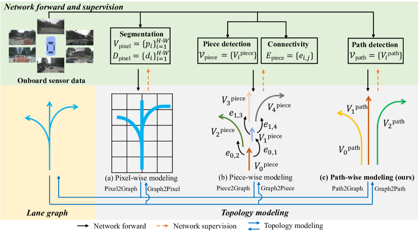
Figure 1: Modeling comparison. (a) Pixel-wise modeling [20] utilizes a predefined Graph2Pixel algorithm to rasterize the lane graph into a segmentation map and a direction map on dense BEV pixels, and heuristic Pixel2Graph post-processing is needed to recover the lane graph from the predicted segmentation map $V_{\text{pixel}}$ and direction map $D_{\text{pixel}}$ (direction map is not drawn here for simplicity). (b) Piece-wise modeling [6] utilizes a predefined Graph2Piece algorithm to split the lane graph into a set of pieces and the connectivity matrix among pieces, and then it merges the predicted pieces $\mathcal{V}_{\text{piece}}$ to the graph with the Piece2Graph algorithm based on predicted connectivity $E_{\text{piece}}$. (c) The proposed path-wise modeling translates the lane graph into continuous and complete paths with a simple predefined Graph2Path algorithm to traverse the graph. We perform path detection and adopt a simple Path2Graph algorithm to recover the lane graph.

We compare LaneGAP with the pixel-wise modeling method HDMapNet [20] and piece-wise modeling methods STSU [6], MapTR [23] under strictly fair conditions (encoder, model size, training schedule, etc.) on the challenging nuScenes [5] and Argoverse2 [41] datasets, which covers diverse graph topology and traffic conditions. With only camera input, LaneGAP achieves the best graph construction quality both quantitatively (see Tab.1) and qualitatively (see Fig. 2), while running at the fastest inference speed. We further push forward the performance of lane graph construction, by introducing the multi-modality input. We believe modeling the lane graph at the path level is reasonable and promising. We hope LaneGAP can serve as a fundamental module of the self-driving system and boost the development of downstream motion planning.

Our contributions can be summarized as follows:

• We propose to model the lane graph in a novel path-wise manner, which well preserves the continuity of the lane and encodes traffic information for planning.

• Based on our path-wise modeling, we present an online lane graph construction method, termed LaneGAP. LaneGAP end-to-end learns the path and constructs the lane graph via the designed Path2Graph algorithm.

• We qualitatively and quantitatively demonstrate the superiority of LaneGAP over pixel-based and piece-based methods. LaneGAP can cope with diverse traffic conditions, especially for road intersections with complicated lane topology.

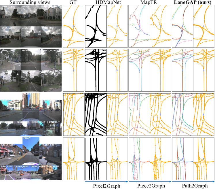
Figure 2: Qualitative comparison of pixel-wise HDMapNet, piece-wise MapTR, and path-wise LaneGAP on the nuScenes and Argoverse2 val splits. Given the 360^∘ horizontal FOV images as input, the proposed path-wise modeling well preserves the continuity across different scenarios, especially for complicated lane topology with more than 4 junction points. The top 2 rows are from the nuScenes val split, and the bottom 2 rows are from the Argoverse2 val split. More visualizations are available in the supplementary material.

2 Related Work

Lane detection.

Lane detection only considers predicting and evaluating the lane divider lines without spatial relation (merging and fork). Since most lane detection datasets only provide front-view images, previous lane detection methods [38, 40, 15, 26, 16, 25] were stuck in predicting lines with a small curvature in a limited horizontal FOV. BezierLaneNet [14] uses a fully convolutional network to predict Bezier lanes defined with 4 Bezier control points. PersFormer [9] proposes a Transformer-based architecture for spatial transformation and unifies 2D and 3D lane detection.

Online HD map construction. Online HD map construction can be seen as an advanced setting of lane detection, consisting of lines and polygons with various semantics in the local 360^∘ FOV perception range of ego-vehicle. With advanced 2D-to-BEV modules [32], previous online HD map construction methods cast it into semantic segmentation task on the transformed BEV features [29, 45, 21, 30, 28, 31]. Building vectorized semantic HD map online achieves increasing interests nowadays [20, 23, 27, 37, 35, 12], HDMapNet [20] follows a segmentation-then-vectorization paradigm. To achieve end-to-end learning [8, 47, 13], VectorMapNet [27] adopts a coarse-to-fine two-stage pipeline for vectorized HD map learning. MapTR [23] proposes unified permutation-equivalent modeling to exploit the undirected nature of semantic HD map and designs a parallel end-to-end framework. BeMapNet [35] and PivotNet [12] propose a Bezier-based representation and pivot-based representation for modeling the map geometry. While the above works focus on the map elements without physical directions (i.e., lane divider, pedstrian crossing and road boundary) and lane graph topology, we aims to fill the gap in this work.

Road graph construction. There is a long history of extracting the road graph from remote sensor data (e.g., aerial imagery and satellite imagery). Many works [33, 46, 2, 19, 4] frame the road graph as a pixel-wise segmentation problem and utilizes morphological post-processing methods to extract the road graph. RoadTracer [1] uses an iterative search process to extract graph topology step by step. Some works [11, 39, 43, 22, 34] follow this sequential generation paradigm. Different from the above works, we focus on the online, ego-centric setting with vehicle-mounted sensors to produce more fine-grained lane-level graph.

Lane graph construction. Lane graph is traditionally constructed with an offline pipeline [42, 18, 3]. [18] proposes a mutli-step training pipeline to construct the lane graph of aerial images based on pixel-wise modeling. [3] proposes a bottom-up approach to aggregate multiple local aerial lane graphs into a global consistent graph. CenterlineDet [42] proposes a DETR-like decision-making transformer network to iteratively update the global lane graph with vehicle-mounted sensors. Recently, STSU [6] shift the offline lane graph construction to the online, ego-centric setting with vehicle-mounted sensors. It models the lane graph as a set of disjoint pieces split by junction points and a set of connections among those pieces. A DETR-like Transformer decoder is proposed to detect those Beizer lane pieces and a successive MLP head is used to predict inter-piece connectivity. Based on STSU, [7] designs a network and utilizes minimal circle extracted by time-consuming offline processing to further supervise the network to produce lane graph. Different from the above graph modelings, we regard the path as the primitive of the lane graph, and model the lane graph in a novel path-wise manner.

3 Method

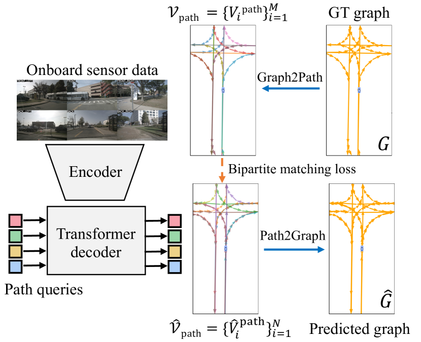
Figure 3: Overview of LaneGAP. Based on the proposed path-wise modeling, LaneGAP first utilizes the Graph2Path algorithm to translate the graph into a set of paths. Then, an end-to-end network is designed to represent and learn the paths. Finally, a Path2Graph algorithm is used to translate the predicted paths into graph structure with negligible cost. Graph2Path and Path2Graph are deterministic algorithms and don’t require backpropagation for optimization.

In this section, we first describe how to translate the directed lane graph into a set of directed paths in Sec. 3.1. Then we introduce the online path detection framework in Sec. 3.2. And we describe how to translate paths back to the lane graph in Sec. 3.3. An overview of our method is exhibited in Fig. 3.

3.1 Graph2Path

Input: directed lane graph $G$

Output: directed paths $\mathcal{V}$

1

2Initialization: $\mathcal{V}\leftarrow\emptyset$, $\text{root vertices set }\Omega_{\text{root}}\leftarrow\emptyset$, $\text{leaf vertices set }\Omega_{\text{leaf}}\leftarrow\emptyset$

3 for vertice in $G$.vertices do

4       if  $\text{vertice}.\text{in\_degree}==0$ then

5             $\Omega_{\text{root}}\leftarrow\Omega_{\text{root}}\cup\{vertice\}$

6            

7       end if

8      if  $\text{vertice}.\text{out\_degree}==0$ then

9             $\Omega_{\text{leaf}}\leftarrow\Omega_{\text{leaf}}\cup\{vertice\}$

10            

11       end if

12      

13 end for

14for root vertice in $\Omega_{\text{root}}$  do

15       for leaf vertice in $\Omega_{\text{leaf}}$ do

16             $V^{\text{path}}=\textbf{findpath}(root\ vertice,leaf\ vertice,G)$

17             if  $V^{\text{path}}\text{ is not None}$ then

18                   $\mathcal{V}\leftarrow\mathcal{V}\cup\{V^{\text{path}}\}$

19                  

20             end if

21            

22       end for

23      

24 end for

25

Return: $\mathcal{V}$

Algorithm 1 Pseudo-code of Graph2Path.

We propose a simple Graph2Path algorithm to translate the directed lane graph into a set of paths according to the direction and connection information encoded in the lane graph. The pseudo-code of Graph2Path is shown in Alg. 1.

Given the ground truth Lane graph $G$, which is typically a directed graph in the local map around the ego-vehicle, we first extract the root vertices $\Omega_{\text{root}}$ and leaf vertices $\Omega_{\text{leaf}}$ based on the indegree and outdegree of vertice. Then we pair the root vertices and leaf vertices (line 2 to 9 in Alg. 1.). For each vertice pair, a depth-first-search (DFS) algorithm is used to find the valid path $V^{\text{path}}$ from the root vertice to the leaf vertice (line 10 to 17 in Alg. 1.). Finally, we can translate the ground truth directed lane graph $G$ to a set of directed paths $\mathcal{V}_{\rm path}=\{V_{i}^{\rm path}\}_{i=1}^{M}$, where $M$ is the number of ground truth paths.

3.2 Path Representation and Learning

Inspired by the advanced set detection methods [8, 47], we propose an end-to-end network, LaneGAP, to predict all paths simultaneously in a single stage, as illustrated in Fig. 3. Our network consists of an encoder that encodes the features from the onboard sensor data, and a query-based Transformer decoder that performs set detection by decoding a set of paths $\hat{\mathcal{V}}_{\rm path}=\{\hat{V}_{i}^{\rm path}\}_{i=1}^{N}$ from the encoded features. To parameterize the path, we utilize two widely-used types of representations, Polyline [27, 23] and Bezier [6, 35], where Polyline offers high flexibility in describing the path, while Bezier provides a smoother representation.

Polyline representation. Polyline representation models the arbitrary directed path as an ordered set of $N_{\text{p}}$ points $V_{\text{poly}}^{\text{path}}=\{p_{j}\in\mathbb{R}^{2}|j=0,1,2,...,N_{\text{p}}-1\}$. We directly regress polyline points and utilize deformable attention [47] to exploit the local information along each Polyline path, where the keys and values are the local features along the Polyline path.

Bezier representation. Bezier representation models the directed path as an ordered set of $N_{\text{b}}$ control points $V_{\text{Bezier}}^{\text{path}}=\{b_{j}\in\mathbb{R}^{2}|j=0,1,2,...,N_{\text{b}}-1\}$. Bezier is a parametric curve, where the point $B$ on the line can be calculated by the weighted sum of control points $V_{\text{Bezier}}^{\text{path}}$:

$$\begin{gathered}B=\sum_{j=0}^{N_{\text{b}}-1}C_{N_{\text{b}}-1}^{j}t^{j}(1-t)^{N_{\text{b}}-1-j}b_{j},0\leq t\leq 1.\end{gathered}$$ (1)

Given the Bezier control points set $V_{\text{Bezier}}^{\text{path}}$ and the sampled interval set $T=\{t_{k}\in\mathbb{R}|0\leq t_{k}\leq 1,k=0,1,2,...,K-1\}$, we can calculate the curve $\mathcal{B}=\{B_{k}\in\mathbb{R}^{2}|0,1,2,...,K-1\}$ with matrix multiplication:

$$\begin{gathered}\mathcal{B}=\Gamma\times V_{\text{Bezier}}^{\text{path}},\end{gathered}$$ (2)

where weight matrix $\Gamma$ is a $K\times N_{\text{b}}$ matrix and $\Gamma(k,j)=C_{N_{\text{b}}-1}^{j}t_{k}^{j}(1-t_{k})^{N_{\text{b}}-1-j}$. For Beizer representation, we use the same network as Polyline representation to regress Bezier control points directly. To enable exploiting the local information along the Bezier path with offline control points, we sample the Bezier path to get online points $\mathcal{B}$ based on Eq. 2 and perform deformable attention, where the keys and values are the local features around the sampled points $\mathcal{B}$ along the Bezier path. We denote this design as Bezier deformable attention, which enables the Transformer decoder to aggregate features along the Bezier path.

Learning. We use the encoder to transform the input onboard sensor data into unified BEV features $F_{\rm BEV}$ [21, 10, 44]. Then we utilize the Transformer decoder to predict a set of paths based on a set of random initialized learnable path queries [23]. With the above path representation, we can cast the predicted path into an ordered set of points with a fixed number $N_{v}$ of points on the path, where $\hat{V}_{i}^{\text{path}}=\{\hat{v}_{j}\in\mathbb{R}^{2}|j=0,1,2,...,N_{v}-1\}$. We modify the bipartite matching loss used in [8] to fit in the path detection setting:

$$\mathcal{L}_{\rm bipartite}(\hat{\mathcal{V}}_{\text{path}},\mathcal{V}_{\text{path}})= \sum_{i=1}^{N}[\mathcal{L}_{\rm{Focal}}(\hat{p}_{{\hat{\sigma}}(i)},c_{i})+$$ (3)

$$\mathds{1}_{\{c_{i}\neq\varnothing\}}\mathcal{L}_{\rm path}(\hat{V}_{\hat{\sigma}(i)}^{\rm path},V_{i}^{\rm path})],$$

$$\mathcal{L}_{\rm path}(\hat{V}_{\hat{\sigma}(i)}^{\rm path},V_{i}^{\rm path})= \sum_{j=0}^{N_{v}-1}L_{1}(\hat{v}_{j},v_{j}),$$

where $\hat{\sigma}$ is the optimal assignment between a set of predicted paths and a set of ground truth paths computed by the Hungarian algorithm, $c_{i}$ is the target class label, and $\mathcal{L}_{\rm{Focal}}(\hat{p}_{{\hat{\sigma}}(i)},c_{i})$ is the classification loss defined in [24]. A $L_{1}$ loss is utilized between the matched predicted path $\hat{V}_{\hat{\sigma}(i)}^{\rm path}$ and sampled ground truth path $V_{i}^{\rm path}$. To enhance the BEV features, we introduce an auxiliary BEV segmentation branch $\phi_{\rm seg}$ to predict the BEV segmentation mask, and the auxiliary BEV segmentation loss is defined as:

$$\begin{gathered}\mathcal{L_{\rm auxseg}}=\mathcal{L_{\rm CE}}(\phi_{\rm seg}(F_{\rm BEV}),M_{\rm BEV}),\end{gathered}$$ (4)

where $M_{\rm BEV}$ is the ground truth. The total loss is defined as:

$$\begin{gathered}\mathcal{L_{\rm total}}=\mathcal{L_{\rm cls}}+\mathcal{L_{\rm path}}+\mathcal{L_{\rm auxseg}},\end{gathered}$$ (5)

where $\mathcal{L_{\rm cls}}$ is the path-wise classification loss using Focal loss [24].

3.3 Path2Graph

Input: a set of paths $\mathcal{V}=\{V_{i}^{\text{path}}\}$

Output: directed lane graph $G$

1

2Initialization: $G=\text{DirGraph}()$

3 for $V^{\text{path}}$ in $\mathcal{V}$ do

4       $V=\{v_{j}\}\leftarrow\textbf{discretize\_path\_to\_vertex\_sequence}(V^{\text{path}})$

5       for  $v_{j}$ in $V$ do

6             if  $v_{j}\ \text{is\ the\ last\ vertice\ of\ }V$ then

7                   $G.\textbf{add\_vertice}(v_{j})$

8                   break

9                  

10             end if

11            $G.\textbf{add\_vertice}(v_{j})$

12             $G.\textbf{add\_edge}(v_{j},v_{j+1})$

13            

14       end for

15      

16 end for

17$G=\textbf{merge\_vertices\_by\_overlap}(G)$

Return: $G$

Algorithm 2 Pseudo-code of Path2Graph.

The predicted continuous paths encode sufficient traffic information and can be directly applied to downstream motion planning. To further recover the graph structure of lane topology and extract merging and fork information, we convert the predicted paths $\hat{\mathcal{V}}=\{\hat{V}_{i}^{\text{path}}\}$ into a directed lane graph $\hat{G}$ with a designed Path2Graph algorithm as shown in Alg. 2.

We discretize the path into point sequences $V=\{v_{j}\}$. The discretized points are regarded as vertices and the adjacent relation between successive points is regarded as edges of vertices. We add these vertices and edges to the directed graph (line 4 to 11 in Alg. 2). The vertices registered in the directed graph $G$ on one path may have spatial overlapping with vertices on other paths. To remove the redundancy of $G$, we merge the overlapped vertices into one vertex (line 13 in Alg. 2).

4 Metrics

Previous works mainly design a network based on one sort of graph modelings (pixel-wise or piece-wise) and choose a metric (pixel-level IoU or instance-level Chamfer distance mAP) friendly to the modeling. To fairly evaluate and compare across different modelings, we adapt the TOPO metric [18] to measure the correctness of the overall directed graph construction. The uniqueness of lane graph construction lies in the junction points, without which the lane graph degenerates into a set of disjoint lanes. To emphasize the quality of the subgraph around the junction points, we propose a new metric, Junction TOPO, which specifically evaluates the accuracy of the local directed graph formed by traversing around the junction points on the directed lane graph.

TOPO metric. Given the predicted directed lane graph $\hat{G}$ and ground truth directed lane graph $G$, we interpolate them so that the distances between any two connected vertices are $0.15m$, and get predicted directed lane graph $\hat{G}=(\hat{V},\hat{E})$ and ground truth directed lane graph $G=(V,E)$ where $\hat{V},V$ are the sets of interpolated vertices and $\hat{E},E$ are the sets of edges among vertices encoding direction and connection. For $\hat{V}$ and $V$, A pair of vertices is considered a candidate match if the distance between the two vertices is less than $0.45m$. And we utilize maximal one-to-one matching among those candidate pairs to find final matched vertices $P_{\text{pair}}=\{(\hat{v},v)_{i}\}_{i=1}^{N_{\text{pair}}}$, then we traverse the directed graph around the paired vertices $\hat{v}$ and $v$ for less than $7.5m$ to get subgraphs $\hat{S}_{\hat{v}}$ and $S_{v}$ on $\hat{G}$ and G. We compute the precision $\text{Pre}(\hat{S}_{\hat{v}},S_{v})=\frac{N_{\text{subpair}}}{|\hat{S}_{\hat{v}}|}$and recall $\text{Rec}(\hat{S}_{\hat{v}},S_{v})=\frac{N_{\text{subpair}}}{|S_{v}|}$ between the vertices of predicted subgraph $\hat{S}_{\hat{v}}$ and the vertices of ground truth subgraph $S_{v}$, where the matching part follows the previous procedure with $0.45m$ threshold. Finally, we report the TOPO precision and recall defined as:

$$\begin{gathered}\text{Precision}_{\text{TOPO}}=\frac{\sum_{i=1}^{N_{\text{pair}}}\text{Pre}(\hat{S}_{\hat{v}},S_{v})}{|\hat{V}|},\\ \text{Recall}_{\text{TOPO}}=\frac{\sum_{i=1}^{N_{\text{pair}}}\text{Rec}(\hat{S}_{\hat{v}},S_{v})}{|V|}.\end{gathered}$$ (6)

Junction TOPO metric. The TOPO metric focuses on the topology correctness of the overall directed lane graph, it does not highlight the correctness of the subgraph formed by traversing from the junction points, which plays a key role in determining the driving choices across different lanes. To bridge this gap, we propose the Junction TOPO metric, which only reports the precision and recall of the junction subgraph. Given the $N_{\text{junction}}$ junction points of the ground truth lane graph, we get pairs of subgraphs $(\hat{S}_{\text{junction}},S_{\text{junction}})$ by traversing the directed graphs $\hat{G}$ and $G$ less than $7.5m$ from junction point. For each subgraph pair, we calculate the precision $\text{Pre}(\hat{S}_{\text{junction}},S_{\text{junction}})$ and recall $\text{Rec}(\hat{S}_{\text{junction}},S_{\text{junction}})$.

Undirected versions. The above metrics calculate the precision and recall by traversing the directed graph $\hat{G}$ and $G$, ignoring the predecessor vertices. To evaluate the complete connections, we turn the directed graphs into undirected graphs and repeat the calculation defined above for two metrics.

5 Experiments

5.1 Dataset

We conduct experiments on two challenging and large-scale datasets, i.e., nuScenes [5] and Argoverse2 [41]. nuScenes [5] dataset consists of 1000 scene sequences. Each sequence is sampled in 2Hz frame rate and provides LiDAR point cloud and RGB images from 6 surrounding cameras, which covers 360^∘ horizontal FOV of the ego-vehicle. The dataset provides the 2D lane graph without height information in the form of lane centerline and covers diverse online driving conditions (e.g., day, night, cloudy, rainy, and occlusion). For the online setting of lane graph construction, we set the perception ranges as $[-15.0m,15.0m]$ for the $X$-axis and $[-30.0m,30.0m]$ for the $Y$-axis and preprocess the dataset following [20, 27, 23]. We train on the nuScenes train set and evaluate on the val set. The experiments on nuScenes dataset are conducted using 6 surrounding-view images by default. Argoverse2 [41] dataset contains 1000 scene logs and 7 surrounding cameras with 360^∘ horizontal FOV. Each log is sampled in 10Hz frame rate and provides 3D lane graph. Due to the disability of pixel-wise modeling in performing 3D segmentation (piece-wise and path-wise modelings can simply predict an extra z corrdinate to support 3D lane graph construction), we drop the height information for fair comparison across different modelings. Other experimental settings are the same as nuScenes.

5.2 Baselines

Dataset	Method	Modeling	Directed Graph						Undirected Graph						Param.	FPS${}_{\text{net}}$
			Junction TOPO			TOPO			Junction TOPO			TOPO
			Prec.	Rec.	$F_{1}$	Prec.	Rec.	$F_{1}$	Prec.	Rec.	$F_{1}$	Prec.	Rec.	$F_{1}$			FPS
nusc	HDMapNet	Pixel-wise	0.594	0.442	0.507	0.608	0.443	0.513	0.526	0.445	0.482	0.563	0.447	0.498	35.4M	17.8	6.8
	STSU	Piece-wise	0.449	0.393	0.419	0.416	0.376	0.395	0.413	0.404	0.408	0.405	0.375	0.389	35.3M	15.8	15.1
	MapTR	Piece-wise	0.540	0.459	0.496	0.504	0.432	0.465	0.493	0.465	0.478	0.487	0.429	0.456	36.0M	15.6	15.0
	LaneGAP(ours)	Path-wise	0.591	0.539	0.564	0.547	0.511	0.529	0.543	0.518	0.530	0.534	0.496	0.514	35.9M	16.5	15.6
av2	HDMapNet	Pixel-wise	0.656	0.449	0.533	0.635	0.463	0.535	0.596	0.473	0.528	0.607	0.470	0.530	35.4M	15.2	4.6
	STSU	Piece-wise	0.562	0.414	0.477	0.462	0.436	0.449	0.512	0.416	0.459	0.449	0.431	0.440	35.3M	13.0	12.4
	MapTR	Piece-wise	0.589	0.469	0.522	0.520	0.481	0.500	0.543	0.468	0.503	0.507	0.477	0.491	36.0M	13.1	12.5
	LaneGAP(ours)	Path-wise	0.663	0.575	0.616	0.578	0.552	0.565	0.627	0.541	0.581	0.569	0.546	0.557	35.9M	13.8	13.0

Table 1: Quantitative comparison of lane graph modeling under fair conditions (the same encoder, comparable model size, the same training schedule, and vision-only modality). FPS${}_{\text{net}}$ and FPS of all the experiments are measured on the same machine with one NVIDIA Geforce RTX 3090 GPU and one 24-core AMD EPYC 7402 2.8 GHz CPU, where FPS${}_{\text{net}}$ is benchmarked with only network forward. Path-wise modeling achieves the best lane graph construction quality and speed.

Implementation details. All the baselines use the same encoder consisting of ResNet50 [17] and GKT [10] to transform the 360^∘ horizontal FOV multi-camera images to the unified BEV features at the resolution of $200\times 100$ (i.e., the BEV grid size is $0.3m$). All the models are controlled in comparable parameter sizes and trained for long enough epochs to ensure convergence (110 epochs on nuScenes and 24 epochs on Argoverse2). We trained all the experiments on 8 NVIDIA GeForce RTX 3090 GPUs with a total batch size of 32 (6 view images on nuScenes and 7 view images on Argoverse2). The only differences lie in the specialized decoders designed for respective modelings, which are detailed as follows.

Pixel-wise modeling. We select HDMapNet [20] as the pixel-wise modeling baseline. It adopts a UNet structure with a ResNet18 to output the binarized segmentation map and direction map with two branches. Meanwhile, a cross-entropy loss is applied to the segmentation map, and $L_{2}$ loss is appled to the (-1,1) normalized direction map [18, 46]. To exclude the quantization error brought by classification on dense pixels, the output resolution of the UNet-shaped [36] segmentation model is set to $400\times 200$, which means the grid size is $0.15m$ (the perception range is $60m\times 30m$) the same as the graph interpolation size.

Piece-wise modeling. STSU [6] is selected as the piece-wise modeling baseline, which consists of a detection branch to detect Bezier lane pieces with 4 control points and a association branch to predict the connectivity between lane pieces. It stacks 6 Transformer decoder layers to iteratively refine the predictions. $L_{1}$ loss is applied to the matched (0,1) normalized pieces and cross-entropy loss is applied to the connectivity. More recently, MapTR [23] proposes a much stronger Transformer decoder for detection branch. We further implement an additional piece-wise baseline by simply replacing the original Beizer piece detection branch of STSU with MapTR Polyline piece detection branch. We set the number of Polyline points to 20.

Path-wise modeling. The path-wise LaneGAP adopts the same decoder as the piece-wise MapTR. We utilize deformable attention [47] as the cross attention of the Transformer and use the 30-point Polyline to represent the path and exploit the features along the path with resort to deformable attention as stated in Sec. 3.2. We stack 6 decoders and regress $(0,1)$ normalized coordinates. During training, $L_{1}$ loss is applied to the matched paths and cross-entropy loss is applied to the auxiliary BEV segmentation branch.

$\mathcal{L}_{\rm auxseg}$	Junction TOPO			TOPO			Param.	FPS
	Prec.	Rec.	$F_{1}$	Prec.	Rec.	$F_{1}$
✗	0.544	0.516	0.529	0.421	0.484	0.450	35.9M	15.6
✓	0.554	0.524	0.539	0.432	0.493	0.461	35.9M	15.6

Table 2: Ablation for auxiliary BEV segmentation branch.

Polyline Points	Junction TOPO			TOPO
	Prec.	Rec.	$F_{1}$	Prec.	Rec.	$F_{1}$
10	0.550	0.515	0.532	0.423	0.481	0.450
30	0.554	0.524	0.539	0.432	0.493	0.461
40	0.566	0.548	0.557	0.440	0.509	0.472

Table 3: Ablation for Polyline path modeling.

Bezier Points	Junction TOPO			TOPO
	Prec.	Rec.	$F_{1}$	Prec.	Rec.	$F_{1}$
3	0.480	0.483	0.481	0.309	0.447	0.365
5	0.514	0.507	0.510	0.375	0.477	0.477
10	0.498	0.503	0.501	0.334	0.463	0.388

Table 4: Ablation for Bezier path representation.

5.3 Quantitative Comparision

Tab. 1 compares path-wise modeling with pixel-wise modeling and piece-wise modeling w.r.t. their accuracy, model size, FPS${}_{\text{net}}$, FPS. All the FPS${}_{\text{net}}$ and FPS are measured on the same machine with one NVIDIA Geforce RTX 3090 GPU and one 24-core AMD EPYC 7402 2.8 GHz CPU, where FPS${}_{\text{net}}$ is benchmarked with only network forward.

Highlights. Path-wise modeling achieves best $F_{1}$ score on the both subgraph around the junction points and the overall graph across two popular datasets (nuScenes and Argoverse2), while running at the fastest inference speed. The designed Path2Graph algorithm has negligible cost in translating predicted paths into directed lane graph (from 16.5 FPS to 15.6 FPS).

Path-wise vs. pixel-wise. Thanks to the high-resolution output of the segmentation model, pixel-wise modeling exhibits comparable precision for sub graph construction and overall graph construction. Nevertheless, the notorious fragmentation and oversmooth issues of segmentation methods make it hard to keep the continuity across pixels and distinguish the fine-grained subgraph around the junction points, leading to much lower recall compared to path-wise modeling. The sophiscated and prone-to-fail post-processing also adds enormous cost at inference to convert the segmentation output into vectorized lane graph. Compared to it, the path-wise modeling demonstrates higher lane graph construction quality and 2x faster inference speed on both nuScenes and Argoverse2 datasets.

Path-wise vs. piece-wise. Path-wise modeling outperforms piece-wise modeling on all metrics (precision, recall, parameter size, FPS). Even euipped with the same advanced Transformer decoder proposed in [23], our path-wise LaneGAP still significantly outperforms piece-wise MapTR, which validates the effectiveness of our proposed continuity-preserving modeling.

5.4 Qualitative Comparison

With the trained models in Tab. 1, Fig. 2 compares path-wise modeling with pixel-wise modeling and piece-wise modeling on complicated lane graphs with more than 4 junction points across different datasets.

Highlights. Path-wise modeling demonstrates better lane graph construction quality than pixel-wise and piece-wise modeling on extremely challenging lane graphs, well preserving the continuity of lane.

Path-wise vs. pixel-wise. As shown in Fig. 2, the pixel-wise HDMapNet performs well on non-junction area. But for the sub-graph around the junction points, the segmentation model struggles to distinguish the fine-grained topology, and the post-processing is prone to fail to generate a decent vectorized lane graph, which aligns with the much lower Junction TOPO metrics in Tab. 1. Thanks to our rational modeling which treats each path as a whole for learning, we can capture the fine-grained topology with severe overlap and preserve the continuity of the lane.

Path-wise vs. piece-wise. The quality of lane graph construted by piece-wise modeling depends on the accuracy of both piece detection and connectivity prediction. As shown in Fig. 2, the piece-wise MapTR either detects jagged lane pieces or produces wrong connections, leading to incomplete and inaccurate lane graph after Piece2Graph post-processing. In contrast, our proposed path-wise modeling encodes the connectivity between pieces into the continuous path representation, which is easy to learn and robust.

5.5 Ablation Study

We ablate the design choices with a 24-epoch training schedule of path-wise modeling on nuScenes dataset by default without specification. And we report Junction TOPO and TOPO only on the directed lane graph.

Effectiveness of auxiliary BEV segmentation branch. Tab. 4 shows the auxiliary BEV segmentation branch can improve the performance by 1% $F_{1}$ of Junction TOPO and 1.1% $F_{1}$ of TOPO without adding cost at inference.

Polyline path representation. As shown in Tab. 4, the performance increases with adding more points for Polyline modeling under a 24-epoch schedule.

Bezier path representation. Tab. 4 shows that adding the number of control points from 3 to 5 improves 2.9% $F_{1}$ of Junction TOPO and 11.2% $F_{1}$ of TOPO, indicating too few Bezier control points cannot accurately describe the arbitrary shape in the broad perception. While adding the number of control points from 5 to 10 incurs an accuracy drop. Compared to Tab. 4, Bezier path representation is inferior to Polyline path representation, so we choose Polyline path representation as the default setting in LaneGAP.

Modality. Tab. 5 shows that LiDAR modality builds a more accurate lane graph than vision modality (6.1% higher $F_{1}$ of Junction TOPO and 4.8% higher $F_{1}$ of TOPO). Fusing them further boosts performance.

Modality	Junction TOPO			TOPO
	Prec.	Rec.	$F_{1}$	Prec.	Rec.	$F_{1}$
Vision-only	0.554	0.524	0.539	0.432	0.493	0.461
LiDAR-only	0.608	0.594	0.600	0.467	0.559	0.509
Vision & LiDAR	0.630	0.600	0.615	0.504	0.561	0.531

Table 5: Ablation for modality.

Training schedule. Tab. 6 shows that adding more epochs mainly increases the TOPO metric and benefits little Junction TOPO, especially the recall of Junction TOPO. The 110-epoch trained multi-modality experiment further pushes the performance of lane graph construction.

Modality	Epoch	Junction TOPO			TOPO
		Prec.	Rec.	$F_{1}$	Prec.	Rec.	$F_{1}$
Vision-only	24	0.554	0.524	0.539	0.432	0.493	0.461
Vision-only	110	0.591	0.539	0.564	0.547	0.511	0.529
Vision & LiDAR	24	0.630	0.600	0.615	0.504	0.561	0.531
Vision & LiDAR	110	0.668	0.601	0.632	0.620	0.576	0.597

Table 6: Ablation for training schedule.

6 Conclusion

In this work, we present an online lane graph construction method LaneGAP based on novel path-wise modeling. We qualitatively and quantitatively demonstrate the superiority of LaneGAP over pixel-based and piece-based methods. LaneGAP can serve as a fundamental module of the self-driving system and facilitate downstream motion prediction and planning, which we leave as future work.

References

- [1] Favyen Bastani, Songtao He, Sofiane Abbar, Mohammad Alizadeh, Hari Balakrishnan, Sanjay Chawla, Sam Madden, and David DeWitt. Roadtracer: Automatic extraction of road networks from aerial images. In CVPR, 2018.
- [2] Anil Batra, Suriya Singh, Guan Pang, Saikat Basu, CV Jawahar, and Manohar Paluri. Improved road connectivity by joint learning of orientation and segmentation. In CVPR, 2019.
- [3] Martin Büchner, Jannik Zürn, Ion-George Todoran, Abhinav Valada, and Wolfram Burgard. Learning and aggregating lane graphs for urban automated driving. In Proceedings of the IEEE/CVF Conference on Computer Vision and Pattern Recognition, pages 13415–13424, 2023.
- [4] Alexander Buslaev, Selim Seferbekov, Vladimir Iglovikov, and Alexey Shvets. Fully convolutional network for automatic road extraction from satellite imagery. In CVPR, 2018.
- [5] Holger Caesar, Varun Bankiti, Alex H Lang, Sourabh Vora, Venice Erin Liong, Qiang Xu, Anush Krishnan, Yu Pan, Giancarlo Baldan, and Oscar Beijbom. nuscenes: A multimodal dataset for autonomous driving. In CVPR, 2020.
- [6] Yigit Baran Can, Alexander Liniger, Danda Pani Paudel, and Luc Van Gool. Structured bird’s-eye-view traffic scene understanding from onboard images. In ICCV, 2021.
- [7] Yigit Baran Can, Alexander Liniger, Danda Pani Paudel, and Luc Van Gool. Topology preserving local road network estimation from single onboard camera image. In CVPR, 2022.
- [8] Nicolas Carion, Francisco Massa, Gabriel Synnaeve, Nicolas Usunier, Alexander Kirillov, and Sergey Zagoruyko. End-to-end object detection with transformers. In ECCV, 2020.
- [9] Li Chen, Chonghao Sima, Yang Li, Zehan Zheng, Jiajie Xu, Xiangwei Geng, Hongyang Li, Conghui He, Jianping Shi, Yu Qiao, and Junchi Yan. Persformer: 3d lane detection via perspective transformer and the openlane benchmark. In ECCV, 2022.
- [10] Shaoyu Chen, Tianheng Cheng, Xinggang Wang, Wenming Meng, Qian Zhang, and Wenyu Liu. Efficient and robust 2d-to-bev representation learning via geometry-guided kernel transformer. arXiv preprint arXiv:2206.04584, 2022.
- [11] Hang Chu, Daiqing Li, David Acuna, Amlan Kar, Maria Shugrina, Xinkai Wei, Ming-Yu Liu, Antonio Torralba, and Sanja Fidler. Neural turtle graphics for modeling city road layouts. In ICCV, 2019.
- [12] Wenjie Ding, Limeng Qiao, Xi Qiu, and Chi Zhang. Pivotnet: Vectorized pivot learning for end-to-end hd map construction. In Proceedings of the IEEE/CVF International Conference on Computer Vision, pages 3672–3682, 2023.
- [13] Yuxin Fang, Bencheng Liao, Xinggang Wang, Jiemin Fang, Jiyang Qi, Rui Wu, Jianwei Niu, and Wenyu Liu. You only look at one sequence: Rethinking transformer in vision through object detection. NeurIPS, 2021.
- [14] Zhengyang Feng, Shaohua Guo, Xin Tan, Ke Xu, Min Wang, and Lizhuang Ma. Rethinking efficient lane detection via curve modeling. In CVPR, 2022.
- [15] Noa Garnett, Rafi Cohen, Tomer Pe’er, Roee Lahav, and Dan Levi. 3d-lanenet: end-to-end 3d multiple lane detection. In ICCV, 2019.
- [16] Yuliang Guo, Guang Chen, Peitao Zhao, Weide Zhang, Jinghao Miao, Jingao Wang, and Tae Eun Choe. Gen-lanenet: A generalized and scalable approach for 3d lane detection. In ECCV, 2020.
- [17] Kaiming He, Xiangyu Zhang, Shaoqing Ren, and Jian Sun. Deep residual learning for image recognition. In CVPR, 2016.
- [18] Songtao He and Hari Balakrishnan. Lane-level street map extraction from aerial imagery. In WACV, 2022.
- [19] Songtao He, Favyen Bastani, Satvat Jagwani, Mohammad Alizadeh, H. Balakrishnan, Sanjay Chawla, Mohamed M. Elshrif, Samuel Madden, and Mohammad Amin Sadeghi. Sat2graph: Road graph extraction through graph-tensor encoding. In ECCV, 2020.
- [20] Qi Li, Yue Wang, Yilun Wang, and Hang Zhao. Hdmapnet: An online hd map construction and evaluation framework. In ICRA, 2022.
- [21] Zhiqi Li, Wenhai Wang, Hongyang Li, Enze Xie, Chonghao Sima, Tong Lu, Yu Qiao, and Jifeng Dai. Bevformer: Learning bird’s-eye-view representation from multi-camera images via spatiotemporal transformers. In ECCV, 2022.
- [22] Zuoyue Li, Jan Dirk Wegner, and Aurélien Lucchi. Topological map extraction from overhead images. In ICCV, 2019.
- [23] Bencheng Liao, Shaoyu Chen, Xinggang Wang, Tianheng Cheng, Qian Zhang, Wenyu Liu, and Chang Huang. MapTR: Structured modeling and learning for online vectorized HD map construction. In ICLR, 2023.
- [24] Tsung-Yi Lin, Priya Goyal, Ross B. Girshick, Kaiming He, and Piotr Dollár. Focal loss for dense object detection. In ICCV, 2017.
- [25] Ruijin Liu, Dapeng Chen, Tie Liu, Zhiliang Xiong, and Zejian Yuan. Learning to predict 3d lane shape and camera pose from a single image via geometry constraints. In AAAI, 2022.
- [26] Ruijin Liu, Zejian Yuan, Tie Liu, and Zhiliang Xiong. End-to-end lane shape prediction with transformers. In WACV, 2021.
- [27] Yicheng Liu, Yue Wang, Yilun Wang, and Hang Zhao. Vectormapnet: End-to-end vectorized hd map learning. arXiv preprint arXiv:2206.08920, 2022.
- [28] Yingfei Liu, Junjie Yan, Fan Jia, Shuailin Li, Qi Gao, Tiancai Wang, Xiangyu Zhang, and Jian Sun. Petrv2: A unified framework for 3d perception from multi-camera images. arXiv preprint arXiv:2206.01256, 2022.
- [29] Zhi Liu, Shaoyu Chen, Xiaojie Guo, Xinggang Wang, Tianheng Cheng, Hongmei Zhu, Qian Zhang, Wenyu Liu, and Yi Zhang. Vision-based uneven bev representation learning with polar rasterization and surface estimation. arXiv preprint arXiv:2207.01878, 2022.
- [30] Zhijian Liu, Haotian Tang, Alexander Amini, Xingyu Yang, Huizi Mao, Daniela Rus, and Song Han. Bevfusion: Multi-task multi-sensor fusion with unified bird’s-eye view representation. arXiv preprint arXiv:2205.13542, 2022.
- [31] Jiachen Lu, Zheyuan Zhou, Xiatian Zhu, Hang Xu, and Li Zhang. Learning ego 3d representation as ray tracing. In ECCV, 2022.
- [32] Yuexin Ma, Tai Wang, Xuyang Bai, Huitong Yang, Yuenan Hou, Yaming Wang, Y. Qiao, Ruigang Yang, Dinesh Manocha, and Xinge Zhu. Vision-centric bev perception: A survey. arXiv preprint arXiv:2208.02797, 2022.
- [33] Gellert Mattyus, Wenjie Luo, and Raquel Urtasun. Deeproadmapper: Extracting road topology from aerial images. In ICCV, 2017.
- [34] Lu Mi, Hang Zhao, Charlie Nash, Xiaohan Jin, Jiyang Gao, Chen Sun, Cordelia Schmid, Nir Shavit, Yuning Chai, and Dragomir Anguelov. Hdmapgen: A hierarchical graph generative model of high definition maps. In CVPR, 2021.
- [35] Limeng Qiao, Wenjie Ding, Xi Qiu, and Chi Zhang. End-to-end vectorized hd-map construction with piecewise bezier curve. In Proceedings of the IEEE/CVF Conference on Computer Vision and Pattern Recognition, pages 13218–13228, 2023.
- [36] Olaf Ronneberger, Philipp Fischer, and Thomas Brox. U-net: Convolutional networks for biomedical image segmentation. In MICCAI, 2015.
- [37] Juyeb Shin, Francois Rameau, Hyeonjun Jeong, and Dongsuk Kum. Instagram: Instance-level graph modeling for vectorized hd map learning. arXiv preprint arXiv:2301.04470, 2023.
- [38] Lucas Tabelini, Rodrigo Berriel, Thiago M Paixao, Claudine Badue, Alberto F De Souza, and Thiago Oliveira-Santos. Keep your eyes on the lane: Real-time attention-guided lane detection. In CVPR, 2021.
- [39] Yong-Qiang Tan, Shang-Hua Gao, Xuan-Yi Li, Ming-Ming Cheng, and Bo Ren. Vecroad: Point-based iterative graph exploration for road graphs extraction. In CVPR, 2020.
- [40] Jinsheng Wang, Yinchao Ma, Shaofei Huang, Tianrui Hui, Fei Wang, Chen Qian, and Tianzhu Zhang. A keypoint-based global association network for lane detection. In CVPR, 2022.
- [41] Benjamin Wilson, William Qi, Tanmay Agarwal, John Lambert, Jagjeet Singh, Siddhesh Khandelwal, Bowen Pan, Ratnesh Kumar, Andrew Hartnett, Jhony Kaesemodel Pontes, et al. Argoverse 2: Next generation datasets for self-driving perception and forecasting. arXiv preprint arXiv:2301.00493, 2023.
- [42] Zhenhua Xu, Yuxuan Liu, Yuxiang Sun, Ming Liu, and Lujia Wang. Centerlinedet: Road lane centerline graph detection with vehicle-mounted sensors by transformer for high-definition map creation. arXiv preprint arXiv:2209.07734, 2022.
- [43] Zhenhua Xu, Yuxiang Sun, and Ming Liu. icurb: Imitation learning-based detection of road curbs using aerial images for autonomous driving. IEEE Robotics and Automation Letters, 6(2):1097–1104, 2021.
- [44] Yan Yan, Yuxing Mao, and Bo Li. Second: Sparsely embedded convolutional detection. Sensors, 18(10):3337, 2018.
- [45] Brady Zhou and Philipp Krähenbühl. Cross-view transformers for real-time map-view semantic segmentation. In CVPR, 2022.
- [46] Lichen Zhou, Chuang Zhang, and Ming Wu. D-linknet: Linknet with pretrained encoder and dilated convolution for high resolution satellite imagery road extraction. In CVPRW, 2018.
- [47] Xizhou Zhu, Weijie Su, Lewei Lu, Bin Li, Xiaogang Wang, and Jifeng Dai. Deformable DETR: deformable transformers for end-to-end object detection. In ICLR, 2021.