A characterization of chains and dancing paths
in dimension three

Abstract.

Given a 3-dimensional CR structure or a path geometry on a surface, its family of chains define a 3-dimensional path geometry. In this article we provide necessary and sufficient conditions that determine whether a path geometry in dimension three arises from chains of a CR 3-manifold or a path geometry on a surface. Moreover, we invariantly characterize 3-dimensional path geometries arising from another family of canonically defined curves for path geometries on surfaces, referred to as dancing paths. We show that chains and dancing paths coincide only in the case of flat path geometries on surfaces. We demonstrate how our characterization can be verified computationally for a given 3-dimensional path geometry and discuss a few examples.

1. Introduction

Geometric structures on manifolds can give rise to distinguished set of curves whose behaviour are of interest in a variety problems. For example, geodesics in (pseudo-)Riemannian geometry or in projective structures, conformal geodesics in conformal geometry, null-geodesics in pseudo-Riemannian conformal geometry, and chains in CR structures or, more generally, in contact parabolic geometries are some of the most well-known cases of such distinguished curves.

The main topic of interest in this article is distinguished curves in 3-dimensional CR structures and 2-dimensional path structures. Such distinguished curves define 3-dimensional (generalized) path geometries. Recall that a (generalized) path geometry is locally defined in terms of a set of paths on a manifold with the property that along each direction in (an open subset of) the tangent space of each point of the manifold, there passes a unique path in that family that is tangent to that direction. For instance, geodesics of an affine connection on a manifold define a path geometry. Path geometries are a generalization of projective structures in which the curves may not be geodesics of any affine connection or satisfy any variational property. More generally, they may not be defined along every direction in each tangent space and may only be defined for an open set of directions at each point.

The first class of distinguished curves that we study are referred to as chains and was originally defined in [CM74] for CR structures. On any CR manifold chains are a canonical family of unparametrized curves with the property that through each point and along each direction transverse to the contact distribution at that point, there passes a unique chain. As a result, chains define a canonical generalized path geometry on any CR manifold. Furthermore, since a 2-dimensional path geometry is defined via a 3-dimensional contact manifold, it can be shown, in a similar manner, that chains can be defined on such contact 3-manifolds as well. As a result, any 2D path geometry or 3D CR geometry defines a canonical 3D path geometry via its chains.

The first objective of this paper is to give a set of invariant conditions for 3-dimensional path geometries which are satisfied if and only if the 3-dimensional path geometry arises from chains of a 3D CR geometry or a 2D path geometry. Our invariant conditions are computationally verifiable, i.e. if a 3-dimensional path geometry is presented either in terms of abstract structure equations or as a pair of second order ODEs, these conditions can be computed by manipulations that involve roots of a binary quartic and differentiation. The steps needed to verify the conditions are explained in detail within the proofs.

Our second objective is to give an in-depth study of another family of distinguished curves canonically defined for any 2-dimensional path geometry and transverse to its contact distribution, referred to as dancing paths, originally due to [BHLN18]. We define dancing path geometries, compare the invariant properties of dancing paths and chains and give an invariant characterization for 3-dimensional path geometries that arise via the dancing construction.

1.1. Outline of the article and main results

In § 2 we give a review of path geometry in dimension 2 and 3. The definition of a (generalized) path geometry on a surface $M$ is given in terms of (an open set of) the 3-dimensional projectivized tangent bundle $\nu\colon\mathbb{P}TM\to M$. Abstractly, a 2-dimensional path geometry is defined via a contact 3-manifolds $N$ with a choice of splitting $\mathscr{C}=\mathscr{D}_{1}\oplus\mathscr{D}_{2}$ of the contact distribution $\mathscr{C}\subset TN$ and, therefore, is denoted by a triple $(N,\mathscr{D}_{1},\mathscr{D}_{2})$. In sufficiently small open sets $U\subset N,$ one can identify $U$ with an open subset of $\mathbb{P}TM$ where $M$ is the leaf space of the integral curves of $\mathscr{D}_{2}.$ We recall local realizability of path geometries in any dimension in terms of point equivalent classes of (systems of) 2nd order ODEs and then discuss the so-called twistor correspondence for path geometries in dimensions 2 and 3. Lastly, we recall the solution of the equivalence problem for these geometric structures. An important feature of 3-dimensional path geometries for us is that their fundamental invariants can be represented as a binary quadric $\mathbf{T},$ referred to as the torsion, and a binary quartic $\mathbf{C},$ referred to as the curvature. As will be discussed in § 2.1, a generalized 3-dimensional path geometry on a 3-manifold $N$ is denoted by a triple $(Q,\mathscr{X},\mathscr{V})$ where $Q$ is 5-dimensional, $\mathscr{X},\mathscr{V}\subset TQ$ intersect trivially and have rank 1 and 2, respectively, their Lie bracket spans $TQ$ everywhere, $\mathscr{V}$ is integrable, and the local 3-dimensional leaf space of the foliation induced by $\mathscr{V}$ on $Q$ is an open set of $N.$

In § 3.1 we define CR structures, recall their corresponding Cartan geometry, and give a Cartan geometric description of chains in 3D CR structures and 2D path structures, following [ČŽ09]. We give a set of necessary conditions for a (generalized) 3-dimensional path geometry on $N,$ i.e. a triple $(Q,\mathscr{X},\mathscr{V}),$ to arise from the chains of a 2-dimensional path geometry $(N,\mathscr{D}_{1},\mathscr{D}_{2}).$ In § 3.2 we describe the 3-dimensional path geometry of chains in these two geometries in terms of the point equivalent class of pairs of second order ODEs. In particular, we discuss the chains of the flat 3D CR structure on 3-sphere $\mathbb{S}^{3}\subset\mathbb{C}^{2}$ and the flat path geometry on $\mathbb{R}\mathbb{P}^{2}$ and the induced (para-)Kähler-Einstein metrics on their respective space of chains, i.e. $\mathrm{SU}(2,1)/\mathrm{U}(1,1)$ and $\mathrm{SL}(3,\mathbb{R})/\mathrm{GL}(2,\mathbb{R})$. In § 3.3 we provide our invariant characterization of chains in Corollary 3.15 for 3D path geometries which involves the algebraic type of the binary quartic $\mathbf{C}$ and the existence of a quasi-symplectic 2-form on the corresponding 5-manifold $Q.$ It follows that $Q$ is an open subset of $\mathbb{P}(TN\backslash\mathscr{C})$ where $\mathscr{C}$ is a contact distribution on a 3-manifold $N$. Recall that a quasi-symplectic 2-form is the odd dimensional analogue of a symplectic 2-form, i.e. a closed 2-form of maximal rank.

Corollary 3.15.

A 3D path geometry $(Q,\mathscr{X},\mathscr{V})$ arises from chains of a 2D path geometry $(N,\mathscr{D}_{1},\mathscr{D}_{2})$ if and only if

1. The binary quartic $\mathbf{C}$ has two distinct real roots of multiplicity 2.

2. The canonical 2-form of rank 2 induced on $Q$ as a result of normalizing $\mathbf{C},$ given in Proposition 3.9, is closed.

3. The entries of the binary quadric $\mathbf{T}$, pulled-back by the bundle inclusion $\iota\colon\mathcal{G}_{D_{r}}\hookrightarrow\mathcal{G}$ in Proposition 3.9, have no dependency on the fibers of $Q\to N$ where $N=Q/\mathscr{V},$

We express the quasi-symplectic 2-form $\rho$ on $Q$ in terms of the Cartan connection of the 3D path geometry on the reduced structure bundle $\mathcal{G}_{D_{r}}\to Q.$ All 3 conditions above are in principle straightforward to check for any 3D path geometry expressed either as a pair of second order ODEs or in terms of abstract structure equations. Moreover, Corollary 3.15 identifies chains as a sub-class of a larger class of 3-dimensional path geometries introduced in Theorem 3.12. We point out in Remark 3.16 that the characterization of path geometry of chains for 2D path geometries is significantly different from the one for higher dimensional (para-)CR structures. In § 3.4 we give an analogous characterization for 3D path geometries arising from chains of 3D CR structures.

Theorem 3.18.

A 3D path geometry $(Q,\mathscr{X},\mathscr{V})$ arises from chains of a 3D CR geometry $(N,\mathscr{C},J)$ if and only if

1. The binary quartic $\mathbf{C}$ has a non-real complex root of multiplicity 2.

2. The canonical 2-form of rank 2 induced on $Q$ as a result of normalizing $\mathbf{C},$ given in Proposition 3.17, is closed.

3. The entries of the binary quadric $\mathbf{T}$, pulled-back by the bundle inclusion $\iota\colon\mathcal{G}_{D_{c}}\hookrightarrow\mathcal{G}$ in Proposition 3.17, have no dependency on the fibers of $Q\to N$ where $N=Q/\mathscr{V},$

In § 4.1 we describe the dancing construction which canonically associates a 3-dimensional path geometry to a 2-dimensional path geometry. Remark 4.6 justifies the terminology of this construction by showing that these 3-dimensional path geometries, via the twistor correspondence, correspond to what is called the dancing construction in [BHLN18, Dun22]. We also discuss the pair of second order ODEs that arise from the dancing paths of a scalar second order ODE. In § 4.2 we give a characterization of dancing path geometries in dimension 3 in the form of Theorem 4.12. As a by-product of Theorem 4.12, in § 4.3 we turn our attention to a natural class of 3-dimensional path geometries that contains dancing path geometries as a proper sub-class, which we refer to as freestyling path geometries. In § 4.4, we provide a characterization of freestyling path geometries in Theorem 4.18. Subsequently, our necessary and sufficient conditions for the dancing construction, as a special case of freestyling, is the content of Corollary 4.31. Since by Proposition 4.23 freestyling path geometries with vanishing torsion coincide with the path geometry of chains for flat 2D path geometries, we restrict ourselves to dancing path geometries with non-zero torsion.

Corollary 4.31.

A 3D path geometry $(Q,\mathscr{X},\mathscr{V})$ with non-zero torsion, i.e. $\mathbf{T}\neq 0,$ arises from a dancing construction applied to a 2D path geometry $(N,\mathscr{D}_{1},\mathscr{D}_{2})$ if and only if

1. The binary quadric $\mathbf{T}$ has two distinct real roots and the binary quartic $\mathbf{C}$ has at least two distinct real roots and no repeated roots.

2. The splitting $\mathscr{V}=\mathscr{V}_{1}\oplus\mathscr{V}_{2}$ defined by the two real roots of $\mathbf{T}$ results in a natural reduction $\iota\colon\mathcal{G}_{T_{G_{r}}}\to\mathcal{G},$ given in Proposition 4.20. There are four integrable rank 2 Pfaffian systems $\iota^{*}\mathcal{I}_{1},\iota^{*}\mathcal{I}_{2},\iota^{*}\mathcal{I}_{3},\iota^{*}\mathcal{I}_{4}$ on $\mathcal{G}_{T_{G_{r}}}$ whose respective leaves project to $Q$ as integral manifolds of rank 3 distributions

   $$\langle\mathscr{X},\mathscr{V}_{2},[\mathscr{X},\mathscr{V}_{2}]\rangle,\quad\langle\mathscr{X},\mathscr{V}_{1},[\mathscr{X},\mathscr{V}_{1}]\rangle,\quad\mathscr{K}_{2}\subset\langle\mathscr{V},[\mathscr{X},\mathscr{V}_{2}]\rangle,\quad\mathscr{K}_{2}\subset\langle\mathscr{V},[\mathscr{X},\mathscr{V}_{1}]\rangle.$$

3. Defining $\tilde{T},\tilde{M},M,T$ to be the local leaf spaces of $\mathcal{I}_{1},\mathcal{I}_{2},\mathcal{I}_{3},\mathcal{I}_{4},$ respectively, they are equipped with 2D path geometries corresponding to $(N,\mathscr{D}_{1},\mathscr{D}_{2}),$ $(N,\tilde{\mathscr{D}}_{1},\mathscr{D}_{2})$ and $(N,\mathscr{D}_{1},\tilde{\mathscr{D}}_{2})$ forming double fibrations

   $$M\leftarrow N\rightarrow T,\qquad M\leftarrow N\rightarrow\tilde{T},\qquad\tilde{M}\leftarrow N\rightarrow T,$$

   respectively. The triple of 2D path geometries above, defined on $N,$ are equivalent.

In Corollary 4.25 we show that flat 2-dimensional path geometries are the only 2D path geometries where the chains define a freestyling which is, in fact, the original dancing construction defined in [BHLN18]. In Remark 4.28 we comment on an interpretation of freestyling as certain intagrability conditions for the induced half-flat causal structure on the 4-dimensional space of its paths. In particular, using Proposition 4.23 and the well-known twistor correspondence between torsion-free path geometries and 4-dimensional self-dual conformal structures, one obtains that a 3-dimensional dancing path geometry corresponds to a conformal structure if and only if the initial 2-dimensional path geometry is flat. Remark 4.32 addresses the dancing construction for higher dimensional integrable Legendrian contact structures.

In Appendix we give the Bianchi identities for the fundamental invariants of 3D path geometries in (A.1), which will be used in the proof of Proposition 3.9. Moreover, we give the structure equations for the reduced 3D path geometries arising from the dancing construction in (A.2) which is discussed in Proposition 4.20.

1.2. Conventions

Our consideration in this paper will be over smooth and real manifold. Throughout the article we always consider path geometry in the generalized sense and therefore will not use the term “generalized” when talking about path geometries. When defining the leaf space of a foliation we always restrict to sufficiently small open sets where the leaf space is smooth and Hausdorff. Consequently, given an integrable distribution $\mathscr{D}$ on a manifold $N,$ by abuse of notation, we denote the leaf space of its induced foliation by $N/\mathscr{D}.$

Given elements $v_{1},\dots,v_{k}$ of a vector space, their span is denoted by $\langle v_{1},\dots,v_{k}\rangle.$ When dealing with differential forms, the algebraic ideal generated by 1-forms $\alpha^{1},\dots,\alpha^{k}$ is denoted as $\{\alpha^{1},\dots,\alpha^{k}\}.$ Given a set of 1-forms $\alpha^{0},\dots,\alpha^{n},\beta^{1},\dots,\beta^{n},$ the corresponding dual frame is denoted as $\frac{\partial}{\partial\alpha^{0}},\cdots\frac{\partial}{\partial\beta^{n}}.$ On a principal bundle $\mathcal{G}\to Q$ with respect to which the 1-forms $\alpha^{0},\dots,\alpha^{n},\beta^{1},\dots,\beta^{n}$ give a basis for semi-basic 1-forms, we define the coframe derivatives of a function $f\colon\mathcal{G}\to\mathbb{R}$ as

$$f_{;i}=\tfrac{\partial}{\partial\alpha^{i}}\lrcorner\,\mathrm{d}f,\ f_{;ij}=\tfrac{\partial}{\partial\alpha^{j}}\lrcorner\,\mathrm{d}f_{;i},\ f_{;\underline{a}}=\tfrac{\partial}{\partial\beta^{a}}\lrcorner\,\mathrm{d}f,\ f_{;\underline{ab}}=\tfrac{\partial}{\partial\beta^{b}}\lrcorner\,\mathrm{d}f_{;\underline{a}},\ f_{;\underline{a}i}=\tfrac{\partial}{\partial\alpha^{i}}\lrcorner\,\mathrm{d}f_{;\underline{a}},\ f_{;i\underline{a}}=\tfrac{\partial}{\partial\beta^{a}}\lrcorner\,\mathrm{d}f_{;i}$$

and similarly for higher orders, where $0\leq i,j\leq n$ and $1\leq a,b\leq n.$ Note that in case we reduce the structure bundle of a geometric structure to a proper principal sub-bundle, by abuse of notation, we suppress the pull-back and use the same notation as above for the coframe derivatives on the reduced bundle.

Lastly, given two distributions $\mathscr{D}_{1}$ and $\mathscr{D}_{2},$ we denote by $[\mathscr{D}_{1},\mathscr{D}_{2}]$ the distribution whose sheaf of sections is $\Gamma([\mathscr{D}_{1},\mathscr{D}_{2}])=\Gamma(\mathscr{D}_{1})+\Gamma(\mathscr{D}_{2})+[\Gamma(\mathscr{D}_{1}),\Gamma(\mathscr{D}_{2})].$ The sheaf of sections of $\bigwedge^{k}(T^{*}M)$ is denoted by $\Omega^{k}(M).$

2. A review of path geometries

In this section we recall some of the well-known facts about path geometries in dimensions two and three including the definition of path geometries, the notion of duality between path geometries on surfaces and a solution for their equivalence problem.

2.1. Definition and realizability as systems of 2nd order ODEs

A path geometry on an $(n+1)$-dimensional manifold $M$ is classically defined as a $2n$-parameter family of paths with the property that along each direction at any point of $M,$ there passes a unique path in that family. Consequently, the natural lift of the paths of a path geometry to the projectivized tangent bundle, $\mathbb{P}TM,$ results in a foliation by curves which are transverse to the fibers $\mathbb{P}T_{x}M.$ It is well-known that a path geometry on an $(n+1)$-dimensional manifold can be locally defined in terms of a system of $n$ second order ODEs

(2.1) $$(z^{i})^{\prime\prime}=F^{i}(t,z,z^{\prime}),\quad t\in\mathbb{R},\ \ z=(z^{1},\dots,z^{n}),\quad 1\leq i\leq n,$$

defined up to point transformations, i.e.

$$t\mapsto\tilde{t}=\tilde{t}(t,z^{1},\ldots,z^{n}),\quad z^{i}\mapsto\tilde{z}^{i}=\tilde{z}^{i}(t,z^{1},\ldots,z^{n}),\quad 1\leq i\leq n.$$

Given a path geometry, its straightforward to see how it defines a system of $n$ 2nd order ODEs: let $(z^{0},\dots,z^{n})$ be local coordinates on $V\subset M$. In a sufficiently small open set $U\subset\mathbb{P}TM,$ the family of paths can be parametrized as $s\mapsto\gamma(s)=(z^{0}(s),\dots,z^{n}(s))$ for $s\in(a,b)\subset\mathbb{R}.$ Each path is determined by the value of $\gamma(s),$ and $\gamma^{\prime}(s)$ at $s=s_{0}\in U,$ thus, taking another derivative, a system of $n+1$ 2nd order ODEs of the form $\gamma^{\prime\prime}=G(\gamma,\gamma^{\prime})$ is obtained for a function $G\colon\mathbb{R}^{2n+2}\to\mathbb{R}^{n+1}.$ If $U\subset\mathbb{P}TM$ is sufficiently small, without loss of generality one can assume $\frac{\mathrm{d}z^{0}}{\mathrm{d}s}\neq 0$ in $U.$ Since the paths are given up to reparametrization, one is able to eliminate $s$ from the system $\gamma^{\prime\prime}=G(\gamma,\gamma^{\prime}).$ As a result, one arrives at the system of ODEs (2.1) where $t:=z^{0}.$

Conversely, starting with an equivalence class of system of $n$ 2nd order ODEs under point transformations (2.1), the system defines a codimension $n$ submanifold $\mathcal{E}\subset J^{2}(\mathbb{R},\mathbb{R}^{n})$ of the 2-jet space $J^{2}(\mathbb{R},\mathbb{R}^{n}).$ Pulling-back the natural contact system on $J^{2}(\mathbb{R},\mathbb{R}^{n})$ to $\mathcal{E},$ one can identify $\mathcal{E}$ with $J^{1}(\mathbb{R},\mathbb{R}^{n})$ which is additionally foliated by contact curves, i.e. the solution curves of the ODE system. Locally, $J^{1}(\mathbb{R},\mathbb{R}^{n})\to J^{0}(\mathbb{R},\mathbb{R}^{n})\cong\mathbb{R}^{n+1}$ can be identified as an open subset of the projectivized tangent bundle $\mathbb{P}TM\to M$ for an $(n+1)$-dimensional manifold $M$ and the solution curves project to a $2n$-parameter family of paths on $M.$ However, for arbitrary ODE systems it may happen that no path is tangent to some directions at some points of $M.$

In fact, there are many instances of path geometries that do not fit the classical description since the paths are only defined along an open set of directions. Thus, in order to study path geometries one is led to work with a generalized notion of such structures as defined below, which is sometimes referred to as generalized path geometry. However, in this article since path geometries for us are always defined in this generalized sense we will not use the term generalized.

Definition 2.1.

An $(n+1)$-dimensional path geometry is given by a triple $(Q,\mathscr{X},\mathscr{V})$ where $Q$ is a $(2n+1)$-dimensional manifold equipped with a pair of distributions $(\mathscr{X},\mathscr{V})$ of rank 1 and $n,$ respectively, which intersect trivially and satisfy $[\mathscr{V},\mathscr{V}]=\mathscr{V}$ and $[\mathscr{X},\mathscr{V}]=TQ$. The $(n+1)$-dimensional local leaf space of the foliation induced by $\mathscr{V}$ is said to be equipped with the path geometry $(Q,\mathscr{X},\mathscr{V})$.

The rank $(n+1)$ distribution $\mathscr{C}$ spanned by $\mathscr{X}$ and $\mathscr{V}$ induces a multi-contact structure on $Q,$ i.e., one can write $\mathscr{C}=\ker\{\alpha^{1},\ldots,\alpha^{n}\}$ for some 1-forms $\alpha^{0},\alpha^{a},\beta^{b},$ such that $\mathscr{X}=\ker\{\alpha^{a},\beta^{b}\}_{a,b=1}^{n},$ $\mathscr{V}=\ker\{\alpha^{0},\ldots,\alpha^{n}\}$ and

$$\mathrm{d}\alpha^{i}\equiv\alpha^{0}{\,{\wedge}\;}\beta^{i}\ \ \mathrm{mod\ \ }\{\alpha^{1},\ldots,\alpha^{n}\},$$

for all $1\leq i\leq n$. Path geometry on surfaces corresponds to $n=1$ in which case $\mathscr{C}$ is a contact distribution on a 3-manifold $N.$ As a result, 2-dimensional path geometries have several unique features that do not extend to higher dimensional path geometries e.g. chains can only be defined for 2-dimensional path geometries.

One can easily check that Definition 2.1 is satisfied for a classical path geometry on an $(n+1)$-dimensional manifold by letting $Q=\mathbb{P}TM$ and $\mathscr{V}$ be the vertical tangent space of the fibration $\mathbb{P}TM\to M$ and $\mathscr{X}$ be the line field tangent to the natural lift of the path on $M$ to $\mathbb{P}TM.$ In terms of the system of second order ODEs (2.1) one has

(2.2) $$\mathscr{X}=\operatorname{span}\left\{\tfrac{\mathrm{D}}{\mathrm{d}t}\right\}\quad\text{where}\quad\tfrac{\mathrm{D}}{\mathrm{d}t}:=\partial_{t}+\sum_{i=1}^{n}p^{i}\partial_{z^{i}}+\sum_{i=1}^{n}F^{i}\partial_{p^{i}},$$

and

$$\mathscr{V}=\operatorname{span}\{\partial_{p^{1}},\ldots,\partial_{p^{n}}\},$$

where $p^{i}$’s are fiber coordinates for an affine chart of $\mathbb{P}TM$. The vector field $\tfrac{\mathrm{D}}{\mathrm{d}t}$ spanning $\mathscr{X}$ is often called the total derivative vector field.

As was mentioned before not all geometries arising from Definition 2.1 are classical path geometries. However, restricting to sufficiently small open sets $U\subset Q$ in Definition 2.1, $U$ can be realized as an open set of $\mathbb{P}TM$ for the $(n+1)$-dimensional manifold $M$ which is the leaf space of $\mathscr{V}.$ Consequently, $\mathscr{X}$ foliates $U\subset\mathbb{P}TM$ by curves that are transverse to the fibers of $\mathbb{P}TM\rightarrow M.$ We refer the reader to [Bry97, Section 2] for more about path geometry on surfaces and [ČS09, Section 4.4.2,4.4.4] for higher dimensions.

2.2. Duality in path geometry on surfaces

Let $(Q,\mathscr{X},\mathscr{V})$ denote a path geometry on the surface $M:=Q/\mathscr{V}$. In this case both $\mathscr{X}$ and $\mathscr{V}$ are of rank 1, and, as we shall explain below, the roles of the two line bundles can be interchanged to define another path geometry, i.e. a dual path geometry. For this reason, in this case we shall use the notation $\mathscr{D}_{1}:=\mathscr{X},$ $\mathscr{D}_{2}:=\mathscr{V},$ and $N:=Q$ to distinguish path geometry on surfaces. Define

$$M=N/\mathscr{D}_{2}$$

to be the leaf space of the foliation induced by $\mathscr{D}_{2}.$ The paths of the induced path geometry on $M$ are projections of integral curves of $\mathscr{D}_{1}$ via the quotient map $\pi_{M}\colon N\to M$. As a result, the paths are parameterized by points of the 2-dimensional leaf space

$$T=N/\mathscr{D}_{1},$$

defined by the quotient map $\pi_{T}\colon N\to T$. The surface $T$ is usually referred to as the twistor space (or the mini-twistor space) of the path geometry on $M$. Thus, given a 2D path geometry $(N,\mathscr{D}_{1},\mathscr{D}_{2}),$ one has the double fibration

$$M\longleftarrow N\longrightarrow T.$$

Similary a 2D path geometry is induced on $T$ for which the paths are the projection of the integral curves of $\mathscr{D}_{2}$. As a result, we get a correspondence between points in $M$ and paths in $T$, and also between paths in $M$ and points in $T$. Furthermore, any point in $N$ is uniquely determined as an intersection point of two integral curves, one tangent to $\mathscr{D}_{1}$ and the other tangent to $\mathscr{D}_{2}$. As a result, any point of $N$ is determined by a path in $M$ with a fixed point on it, or, equivalently, by a path in $T$ with a fixed point on it. This extends the flat model of the 2-dimensional path geometry where $M$ and $T$ are given by 2-dimensional projective spaces $\mathbb{R}\mathbb{P}^{2}$ and $(\mathbb{R}\mathbb{P}^{2})^{*}$ and $N$ is the 3-dimensional space of flags of a line inside a plane in $\mathbb{R}^{3}$ which is equivalent to the space of marked projective lines in $\mathbb{P}^{2}.$ The 3-manifold $N$ is usually referred to as the correspondence space and can be viewed via the inclusion

$$N\subset M\times T.$$

On the level of ODEs the correspondence between $M$ and $T$ gives rise to the Cartan duality for second order ODEs, which from the viewpoint of the geometry on $N$ simply interchange the role of $\mathscr{D}_{1}$ and $\mathscr{D}_{2}$. Namely, picking coordinates $(t,z)$ on $M$ and $(\tilde{t},\tilde{z})$ on $T$ one gets a second order ODE on $M$

(2.3) $$\frac{\mathrm{d}^{2}z}{\mathrm{d}t^{2}}=F\left(t,z,\frac{\mathrm{d}z}{\mathrm{d}t}\right)$$

whose solutions are paths on $M$, and, similarly, a second order ODE on $T$

(2.4) $$\frac{\mathrm{d}^{2}\tilde{z}}{\mathrm{d}\tilde{t}^{2}}=\tilde{F}\left(\tilde{t},\tilde{z},\frac{\mathrm{d}\tilde{z}}{\mathrm{d}\tilde{t}}\right),$$

whose solutions are paths on $T$. The two scalar second order ODEs (2.3) and (2.4), or more precisely, their point equivalence classes, and the corresponding path geometries, are called dual to each other. Notice that $T$ is the solutions space for (2.3) and $M$ is the solution space for (2.4).

More generally one can write solutions of either (2.3) or (2.4) in the following implicit form

$$\Phi(t,z,\tilde{t},\tilde{z})=0$$

where $\Phi$ is a function on $M\times T$. Fixing $\tilde{t}=\mathrm{const}$, $\tilde{z}=\mathrm{const}$ we get a curve in $M$, and, conversely, fixing $t=\mathrm{const}$, $z=\mathrm{const}$ we get a curve in $T$. Then, the aforementioned inclusion $N\subset M\times T$ is realized as

$$N=\{(t,z,\tilde{t},\tilde{z})\in M\times T\ |\ \Phi(t,z,\tilde{t},\tilde{z})=0\}.$$

Using the notion of duality of 2-dimensional path geometries, we give the following definition.

Definition 2.2.

A path geometry on $M$ is called a projective structure if its paths coincide with the geodesics of a linear connection $\nabla$ on $M$ as unparametrized curves. A path geometry on $M$ is called a co-projective structure if its dual path geometry is a projective structure.

2.3. Solution of the equivalence problem

Two path geometries $(Q_{i},\mathscr{X}_{i},\mathscr{V}_{i}),i=1,2$ are called equivalent if there exists a bundle diffeomorphism $f\colon Q_{1}\to Q_{2}$ such that $f_{*}(\mathscr{X}_{1})=\mathscr{X}_{2}$ and $f_{*}(\mathscr{V}_{1})=\mathscr{V}_{2}.$ We point out that a 2-dimensional path geometry is not in general equivalent to its dual.

To determine when two path geometries are locally equivalent, we provide a solution to the equivalence problem of path geometries using the notion of a Cartan geometry and Cartan connection as defined below.

Definition 2.3.

Let $G$ be a Lie group and $P\subset G$ a Lie subgroup with Lie algebras $\mathfrak{g}$ and $\mathfrak{p}\subset\mathfrak{g},$ respectively. A Cartan geometry of type $(G,P)$ on $Q,$ denoted as $(\mathcal{G}\to Q,\psi),$ is a right principal $P$-bundle $\tau\colon\mathcal{G}\to Q$ equipped with a Cartan connection $\psi\in\Omega^{1}(\mathcal{G},\mathfrak{g}),$ i.e. a $\mathfrak{g}$-valued 1-form on $\mathcal{G}$ satisfying

1. $\psi$ is $P$-equivariant, i.e. $r_{g}^{*}\psi=\mathrm{Ad}_{g^{-1}}\circ\psi$ for all $g\in P.$

2. $\psi_{z}\colon T_{z}\mathcal{G}\to\mathfrak{g}$ is a linear isomorphism for all $z\in\mathcal{G}.$

3. $\psi$ maps fundamental vector fields to their generators, i.e. $\psi(\zeta_{X})=X$ for any $X\in\mathfrak{p}$ where $\zeta_{X}(z):=\frac{\mathrm{d}}{\mathrm{d}t}\,\vline_{\,t=0}r_{exp(tX)}(z).$

The 2-form $\Psi\in\Omega^{2}(\mathcal{G},\mathfrak{g})$ defined as

$$\Psi(u,v)=\mathrm{d}\psi(u,v)+[\psi(X),\psi(Y)]\quad\text{for\ \ }X,Y\in\Gamma(T\mathcal{G}),$$

is called the Cartan curvature and is $P$-equivariant and semi-basic with respect to the fibration $\mathcal{G}\to Q.$

The following solution of the equivalence problem for path geometries is due to Cartan [Car24] for surfaces and due to Grossman and Fels [Gro00, Fel95] in higher dimensions.

Theorem 2.4.

Every path geometry $(Q^{2n+1},\mathscr{X},\mathscr{V}),$ as in Definition 2.1, defines Cartan geometry $(\mathcal{G}\to Q,\psi)$ of type $(\mathrm{PSL}(n+2,\mathbb{R}),P_{12})$ where $P_{12}\subset\mathrm{PSL}(n+2,\mathbb{R})$ is the parabolic subgroup preserving the flag of a line and a 2-plane in $\mathbb{R}^{n+3}.$ Assume that the distributions $\mathscr{X}$ and $\mathscr{V}$ are the projection of the distributions $\ker\{\alpha^{i},\beta^{i}\}_{i=1}^{n}$ and $\ker\{\alpha^{i}\}_{i=0}^{n},$ respectively. When $n\geq 2$, the Cartan connection and its curvature can be expressed as

(2.5) $$\psi=\begin{pmatrix}-\psi^{i}_{i}-\psi^{0}_{0}&\mu_{0}&\mu_{j}\\ \alpha^{0}&\psi^{0}_{0}&\nu_{j}\\ \alpha^{i}&\beta^{i}&\psi^{i}_{j}\\ \end{pmatrix}\quad\mathrm{and}\quad\Psi:=\mathrm{d}\psi+\psi{\,{\wedge}\;}\psi=\begin{pmatrix}0&M_{0}&M_{j}\\ 0&\Psi^{0}_{0}&V_{j}\\ 0&B^{i}&\Psi^{i}_{j}\\ \end{pmatrix},$$

where $1\leq i,j\leq n$ and

$$B^{i}=T^{i}_{j}\alpha^{0}{\,{\wedge}\;}\alpha^{j}+\textstyle{\frac{1}{2}}T^{i}_{jk}\alpha^{j}{\,{\wedge}\;}\alpha^{k},\qquad\mathrm{and}\quad\Psi^{i}_{j}=C^{i}_{jkl}\alpha^{k}{\,{\wedge}\;}\beta^{l}+\textstyle{\frac{1}{2}}T^{i}_{jkl}\alpha^{k}{\,{\wedge}\;}\alpha^{l}+T^{i}_{j0k}\alpha^{0}{\,{\wedge}\;}\alpha^{k}.$$

The fundamental invariants of a path geometry are the torsion, $\mathbf{T}=(T^{i}_{j})_{1\leq i,j\leq n},$ and the curvature, $\mathbf{C}=(C^{i}_{jkl})_{1\leq i,j,k,l\leq n}$, satisfying

(2.6) $$T^{i}_{i}=0,\qquad C^{i}_{jkl}=C^{i}_{(jkl)},\qquad C^{i}_{ijk}=0.$$

Remark 2.5.

We point out that unlike in § 2.1, the 1-forms in Theorem 2.4 are defined on the principal bundle $\mathcal{G}$ rather than the manifold $Q.$ If it is clear from the context that one needs to take a section $s\colon Q\to\mathcal{G}$ and consider $s^{*}\psi,$ we will not make a distinction between 1-forms defined on $\mathcal{G}$ or $Q.$

If $(t,z^{i})$ and $(t,z^{i},p^{i})$ are local jet coordinates on $\mathbb{R}\times\mathbb{R}^{n}=J^{0}(\mathbb{R},\mathbb{R}^{n})$ and $J^{1}(\mathbb{R},\mathbb{R}^{n}),$ respectively, then in terms of the system of ODEs (2.1), one obtains

(2.7) $$T^{i}_{j}=F^{i}_{j}-\textstyle{\frac{1}{2}\delta^{i}_{j}F^{k}_{k}},\qquad\qquad C^{i}_{jkl}=F^{i}_{jkl}-\textstyle{\frac{3}{4}}F^{r}_{r(jk}\delta^{i}_{l)}$$

where $1\leq i,j,k,l\leq n$ and

(2.8) $$F^{i}_{j}=\textstyle{-F^{i}_{z^{j}}+\frac{1}{2}\textstyle{\frac{\mathrm{D}}{\mathrm{d}t}}(F^{i}_{p^{j}})-\frac{1}{4}F^{i}_{p^{k}}F^{k}_{p^{j}},}\quad F^{i}_{jkl}=F^{i}_{p^{j}p^{k}p^{l}},\quad\textstyle{\frac{\mathrm{D}}{\mathrm{d}t}}=\partial_{t}+p^{i}\partial_{z^{i}}+F^{i}\partial_{p^{i}}.$$

Cartan’s solution of the equivalent problem for path geometries on surfaces is as follows.

Theorem 2.6.

Given a 2-dimensional path geometry $(N,\mathscr{D}_{1},\mathscr{D}_{2})$ it defines a Cartan geometry $(\mathcal{P}\to N,\phi)$ of type $(\mathrm{SL}(3,\mathbb{R}),P_{12})$ where $P_{12}$ is the subgroup of upper diagonal matrices and

(2.9) $$\phi=\begin{pmatrix}-\phi^{i}_{i}&\theta_{2}&\theta_{0}\\ \omega^{1}&\phi^{1}_{1}&\theta_{1}\\ \omega^{0}&\omega^{2}&\phi^{2}_{2}\\ \end{pmatrix}.$$

The Cartan curvature of $\phi$ is given by

(2.10) $$\begin{pmatrix}0&T_{1}\omega^{0}{\,{\wedge}\;}\omega^{1}&T_{2}\omega^{0}{\,{\wedge}\;}\omega^{1}+C_{2}\omega^{0}{\,{\wedge}\;}\omega^{2}\\ 0&0&C_{1}\omega^{0}{\,{\wedge}\;}\omega^{2}\\ 0&0&0\end{pmatrix}$$

for some functions $T_{1},T_{2},C_{1},C_{2}$ on $\mathcal{P}$ where $\mathbf{T}=T_{1}$ and $\mathbf{C}=C_{1}$ are the fundamental invariants.

More explicitly, since 2D path geometries correspond to point equivalence classes of scalar 2nd order ODEs, given a scalar ODE

$$z^{\prime\prime}=F(t,z,z^{\prime}),$$

one obtains

$$T_{1}=\tfrac{\mathrm{D^{2}}}{\mathrm{d}t^{2}}F_{z^{\prime}z^{\prime}}-4\tfrac{\mathrm{D}}{\mathrm{d}t}F_{zz^{\prime}}-F_{z^{\prime}}\tfrac{\mathrm{D}}{\mathrm{d}t}F_{z^{\prime}z^{\prime}}+4F_{z^{\prime}}F_{zz^{\prime}}-3F_{z}F_{z^{\prime}z^{\prime}}+6F_{zz},\quad C_{1}=F_{z^{\prime}z^{\prime}z^{\prime}z^{\prime}}$$

Here we are interested in path geometries on 3-dimensional manifolds, i.e. $Q$ in Definition 2.1 is 5-dimensional, which correspond to point equivalence classes of pairs of 2nd order ODEs. The following proposition will be important for us whose proof is straightforward and will be skipped.

Proposition 2.7.

In three-dimensional path geometries the fundamental invariants $\mathbf{T}$ and $\mathbf{C}$ in Theorem 2.4, as $\mathrm{GL}_{2}(\mathbb{R})$-modules can be represented as a binary quadric and a binary quartic, respectively, given by

(2.11) $$\mathbf{T} =s^{*}(A_{0}(\beta^{1})^{2}+2A_{1}\beta^{1}\beta^{2}+A_{2}(\beta^{2})^{2})\otimes V\otimes X^{-2},$$

$$\mathbf{C} =s^{*}(W_{0}(\beta^{1})^{4}+4W_{1}(\beta^{1})^{3}(\beta^{2})+6W_{2}(\beta^{1})^{2}(\beta^{2})^{2}+4W_{3}(\beta^{1})(\beta^{2})^{3}+W_{4}(\beta^{2})^{4})\otimes V\otimes X^{-1}$$

where $s\colon Q\to\mathcal{G}$ is a section, $\mathbf{T}\in\Gamma(\mathrm{Sym}^{2}(\mathscr{V}^{*})\otimes\bigwedge^{2}\mathscr{V}\otimes\mathscr{X}^{-2}),$ $\mathbf{C}\in\Gamma(\mathrm{Sym}^{4}(\mathscr{V}^{*})\otimes\bigwedge^{2}\mathscr{V}\otimes\mathscr{X}^{-1}),$ $X:=\frac{\partial}{\partial s^{*}\alpha^{0}}\in\Gamma(\mathscr{X}),$ $V:=\frac{\partial}{\partial s^{*}\beta^{1}}{\,{\wedge}\;}\frac{\partial}{\partial s^{*}\beta^{2}}\in\Gamma(\bigwedge^{2}\mathscr{V}),$

$$\begin{gathered}A_{0}=T^{2}_{1},\quad A_{1}=T^{2}_{2},\quad A_{2}=-T^{1}_{2},\\ W_{0}=C^{2}_{111},\quad W_{1}=C^{2}_{211},\quad W_{2}=C^{2}_{221},\quad W_{3}=C^{2}_{222},\quad W_{4}=-C^{1}_{222},\end{gathered}$$

and $(\tfrac{\partial}{\partial s^{*}\alpha^{0}},\tfrac{\partial}{\partial s^{*}\alpha^{1}},\tfrac{\partial}{\partial s^{*}\alpha^{2}},\tfrac{\partial}{\partial s^{*}\beta^{1}},\tfrac{\partial}{\partial s^{*}\beta^{2}})$ denote the vector fields dual to the coframe $s^{*}(\alpha^{0},\alpha^{1},\alpha^{2},\beta^{1},\beta^{2})$ in the Cartan connection (2.5). Moreover, $Q$ is equipped with a degenerate conformal structure given by $[s^{*}h]\subset\mathrm{Sym^{2}}(T^{*}Q)$ where

(2.12) $$h:=\alpha^{1}\beta^{2}-\alpha^{2}\beta^{1}\in\Gamma(\mathrm{Sym}^{2}(T^{*}\mathcal{G})).$$

Using Theorems 2.4 and 2.6, it follows that two path geometries $(Q_{i},\mathscr{X}_{i},\mathscr{V}_{i}),i=1,2$ are locally equivalent if and only if for their respective Cartan geometries $(\mathcal{G}_{i}\to Q_{i},\psi_{i})$ there is a diffeomorphism $f\colon\mathcal{G}_{1}\to\mathcal{G}_{2}$ such that $f^{*}\psi_{2}=\psi_{1}.$

Furthermore, if the fundamental invariants vanish, i.e. $\mathbf{C}=\mathbf{T}=0,$ then the Cartan curvature is zero and the Cartan connection coincides with the Maurer-Cartan forms on $\mathrm{PSL}(n+2,\mathbb{R})$ and the path geometry is locally equivalent to the canonical one on $\mathbb{R}\mathbb{P}^{n+1}$ whose paths are projective lines. If $\mathbf{C}=0,$ then the path geometry defines a projective structure on the $(n+1)$-dimensional leaf space of $\mathscr{V},$ denoted by $M.$ If $\mathbf{T}=0,$ then the $2n$-dimensional leaf space of $\mathscr{X}$, i.e. the solution space of the corresponding system of ODEs, is endowed with a so-called $\beta$-integrable Segré structure if $n\geq 2$ and a projective structure if $n=1$.

Note that when $n=2$ and $\mathbf{T}=0,$ then the induced $\beta$-integrable Segré structure on the leaf space of $\mathscr{X},$ is a 4-dimensional half-flat conformal structure which is defined by the conformal class of the bilinear form $h$ in Proposition 2.7. In this case $\mathbf{C}$ coincides with the binary quartic representation of the self-dual Weyl curvature of the induced conformal structure.

Lastly we recall the notion of orientability for path geometries on surfaces, following [Bry97, Section 2]. A path geometry on a surface given by $(N,\mathscr{D}_{1},\mathscr{D}_{2})$ is said to be oriented if the leaves of $\mathscr{D}_{1}$ and $\mathscr{D}_{2}$ can be endowed with a continuous choice of orientation. This is equivalent to the existence of two non-vanishing vector fields $v_{i}\in\Gamma(\mathscr{D}_{i})$ on $N.$ A 1-form $\alpha$ is called $\mathscr{D}_{i}$-positive if its pull-back to each leaf of $\mathscr{D}_{i}$ is positive with respect to a pre-assigned orientation. As a result, by the naturally induced co-orientation on the contact distribution due to the relation $\mathrm{d}\omega^{0}\equiv\omega^{1}{\,{\wedge}\;}\omega^{2}$ mod $\{\omega^{0}\},$ having $\mathscr{D}_{i}$-positive 1-forms $\omega^{1}$ and $\omega^{2}$ determines an orientation on $N.$ Since by definition the fibers of $N\to M$ and $N\to T$ are connected, it is straightforward to show that an oriented path geometry determines an orientation on the leaf spaces of $\mathscr{D}_{1}$ and $\mathscr{D}_{2}.$ Similarly, one can define oriented path geometries $(Q,\mathscr{X},\mathscr{V})$ in higher dimensions by assigning a continuous choice of orientation to the leaves of $\mathscr{X}$ and $\mathscr{V}$ which imply the existence of a nonvanishing vector field spanning $\mathscr{X}$ and a nonvanishing section of $\bigwedge^{n}(\mathscr{V}).$ As in the case of surfaces, via the multi-contact structure, one obtains an orientation on the leaf space of the foliation induced by $\mathscr{V}.$

3. Chains

In this section we will discuss chains in 3-dimensional CR structures and 2-dimensional path geometries. We review known facts about chains and derive necessary conditions for a 3-dimensional path geometry defined by chains. We describe such path geometries in terms of their corresponding point equivalent class of pairs of second order ODEs. We finish by describing our characterization of chains as a subclass of a larger set of 3-dimensional path geometries.

3.1. Chains in 3D CR geometry and 2D path geometry

In this section we recall the definition of a 3D CR structure and chains in CR and 2D path geometries. We finish by giving necessary conditions for a 3D path geometry that is defined by chains.

Definition 3.1.

A non-degenerate CR structure of hypersurface type on an $(2n+1)$-dimensional manifold $M$ is given by a contact distribution $\mathscr{C}\subset TN$ with an integrable almost complex structure $J\colon\mathscr{C}\to\mathscr{C}$ such that $\mathfrak{L}(JX,JY)=\mathfrak{L}(X,Y)$ where $\mathfrak{L}_{x}:(X,Y)\to[X,Y]_{x}/\mathscr{C}_{x}\in T_{x}N/\mathscr{C}_{x}$ for $X,Y\in\Gamma(TN)$ is the Levi bracket.

Identifying $TN/\mathscr{C}$ at each point $x\in N$ with $\mathbb{R},$ the map $\mathfrak{L}_{x}$ corresponds to the imaginary part of a Hermitian inner product of signature $(p,q),p+q=n.$ The induced action of $J$ on $\mathbb{C}\mathscr{C}:=\mathbb{C}\otimes\mathscr{C}$ results in the splitting $\mathbb{C}\mathscr{C}=\mathscr{H}\oplus\bar{\mathscr{H}},$ where $\mathscr{H}$ and $\bar{\mathscr{H}}$ are holomorphic and anti-holomorphic sub-bundles of $\mathscr{C}$ for the complex structure defined by $J,$ respectively. Two CR structures, denoted as $(N_{i},\mathscr{C}_{i},J_{i}),i=1,2$ are equivalent if there is a diffeomorphism $F\colon N_{1}\to N_{2}$ whose pushforward $F_{*}\colon TN_{1}\to TN_{2}$ and its extension to $\mathbb{C}\otimes TN_{1}$ satisfy $F_{*}\mathscr{C}_{1}=\mathscr{C}_{2}$ and $F_{*}\mathscr{H}_{1}=\mathscr{H}_{2}$ where $\mathscr{H}_{i}$ are the holomorphic sub-bundles of $\mathscr{C}_{i}$ with respect to $J_{i}.$ Similarly, one can define local equivalence of two CR structures at two points by finding such a diffeomorphism in sufficiently small neighborhoods of those points.

Restricting to 3-dimensional CR structures, the following theorem of Cartan gives a solution of the equivalence problem in terms of a Cartan geometry. We refer the reader to [Jac90, Bry04, ČS09] for more background on the geometry of CR structures.

Theorem 3.2 (Cartan [Car32, Car33]).

A 3-dimensional CR structure is a Cartan geometry $(\mathcal{P}\to N,\phi)$ of type $(\mathrm{SU}(2,1),P)$ where $P$ is the stabilizer of a non-zero null line in $\mathbb{C}^{3}.$ Expressing the Cartan connection as

(3.1) $$\phi=\begin{pmatrix}-\phi_{0}-\tfrac{1}{3}\mathrm{i}\phi_{1}&\mathrm{i}\theta&\mathrm{i}\theta_{0}\\ \bar{\omega}&\tfrac{2}{3}\mathrm{i}\phi_{1}&-\mathrm{i}\bar{\theta}\\ \mathrm{i}\omega^{0}&\omega&\phi_{0}-\tfrac{1}{3}\mathrm{i}\phi_{1}\end{pmatrix},\quad\omega=\omega^{1}+\mathrm{i}\omega^{2},\quad\theta=\theta_{1}+\mathrm{i}\theta_{2}.$$

which is $\mathfrak{su}(2,1)$-valued with respect to the Hermitian form $H$ in three variables

$$H(Z)=Z_{3}\bar{Z}_{1}-Z_{2}\bar{Z}_{2}+Z_{1}\bar{Z}_{3},\quad Z=(Z_{1},Z_{2},Z_{3})\in\mathbb{C}^{3},$$

the Cartan curvature is given by

(3.2) $$\Phi=\mathrm{d}\phi+\phi{\,{\wedge}\;}\phi=\begin{pmatrix}0&R\omega^{0}{\,{\wedge}\;}\omega&\mathrm{i}(S\omega^{0}{\,{\wedge}\;}\omega+\bar{S}\omega^{0}{\,{\wedge}\;}\bar{\omega})\\ 0&0&\bar{R}\omega^{0}{\,{\wedge}\;}\bar{\omega}\\ 0&0&0\end{pmatrix},\quad R=R_{1}+\mathrm{i}R_{2},\quad S=S_{1}+\mathrm{i}S_{2}.$$

for two complex-valued functions $R$ and $S$ on $\mathcal{P}.$ The vanishing of $R$ implies that $\Phi=0$ and that the CR structure is locally equivalent to the hyperquadric $\Im(w)=\tfrac{1}{4}z\bar{z}$ in $\mathbb{C}^{2}$ where $(z,w)$ are local coordinates on $\mathbb{C}^{2}.$

Note that the 3-dimensional hyperquadric in $\mathbb{C}^{2}$ is a graph for the compact quadric $z_{0}\bar{z}_{2}-z_{1}\bar{z}_{1}+z_{2}\bar{z}_{0}=0$ in $\mathbb{C}\mathbb{P}^{2}$ where $[z_{0}\colon z_{1}\colon z_{2}]$ are homogeneous coordinates using which $\mathbb{C}^{2}$ is identified as $[1\colon z_{1}\colon z_{2}]$. It can be shown, e.g. see [Jac90, Section 2.2], that it is CR equivalent to the 3-sphere $\mathbb{S}^{3}\subset\mathbb{C}^{2}$ given by $w\bar{w}+z\bar{z}=1$.

The grading of $\mathfrak{su}(2,1)$ that corresponds to the parabolic subgroup $P$ is a contact grading, i.e.

$$\mathfrak{su}(2,1)=\mathfrak{g}_{-2}\oplus\mathfrak{g}_{-1}\oplus\mathfrak{g}_{0}\oplus\mathfrak{g}_{1}\oplus\mathfrak{g}_{2},$$

where, in terms of (3.1), $\omega^{0}\in\mathfrak{g}_{-2},$ $\omega,\bar{\omega}\in\mathfrak{g}_{-1},$ $\phi_{1},\phi_{2}\in\mathfrak{g}_{0},$ $\theta,\bar{\theta}\in\mathfrak{g}_{1},$ and $\theta_{0}\in\mathfrak{g}_{2}.$ Now we can define chains as follows.

Definition 3.3.

Let $(N,\mathscr{C},J)$ be a 3-dimensional CR structure with Cartan geometric data $(\mathcal{P}\to N,\phi).$ Fixing a contact grading of $\mathfrak{su}(2,1)$ and taking any $X\in\mathfrak{g}_{-2},$ a chain on $N$ is a curve that is the projection of an integral curve of the vector field $\phi^{-1}(X)\in\Gamma(T\mathcal{P})$ via the projection $\tau\colon\mathcal{P}\to N.$

Using the Cartan geometric description of CR structures, in [ČŽ09] the path geometry of their chains was studied, which we recall briefly in the case of 3D CR structures. Firstly, one starts by describing the set of transverse directions to the contact distribution. Let $S\subset P$ be the stabilizer of the line $l\subset\mathfrak{su}(2,1)$ spanned by an element of $\mathfrak{g}_{-2}.$ It follows that $\mathfrak{s}=\mathfrak{g}_{0}\oplus\mathfrak{g}_{2}\subset\mathfrak{p}=\mathfrak{g}_{0}\oplus\mathfrak{g}_{1}\oplus\mathfrak{g}_{2}$ where $\mathfrak{s}$ and $\mathfrak{p}$ are the Lie algebras of $S$ and $P,$ respectively. Moreover, it is straightforward to see that the $P$-orbit of $l,$ denotes as $P\cdot l\subset\mathfrak{su}(2,1)/\mathfrak{p},$ is the set of all lines in $\mathfrak{su}(2,1)/\mathfrak{p}$ that are not contained in $\mathfrak{g}^{-1}/\mathfrak{p}$ where $\mathfrak{g}^{-1}:=\mathfrak{g}_{-1}\oplus\mathfrak{g}_{0}\oplus\mathfrak{g}_{1}\oplus\mathfrak{g}_{2}$ and $\mathcal{P}\times_{P}\mathfrak{g}^{-1}/\mathfrak{p}$ is the contact distribution $\mathscr{C}\subset TN.$ Thus, the bundle of directions that are transverse to the contact distribution, i.e. $Q:=\mathbb{P}(TN\backslash\mathscr{C}),$ can be identified with $\mathcal{P}/S:=\mathcal{P}\times_{P}P/S.$ Viewing the Cartan connection $\phi\in\Omega^{1}(\mathcal{P},\mathfrak{su}(2,1))$ as a connection on $Q,$ it gives

$$TQ\cong\mathcal{P}\times_{S}(\mathfrak{su}(2,1)/\mathfrak{s}).$$

Using the above identification, it follows that the induced path geometry $(Q,\mathscr{X},\mathscr{V})$ is give by $\mathscr{X}=\nu_{*}(\phi^{-1}(\mathfrak{g}_{-2}))$ and $\mathscr{V}=\nu_{*}(\phi^{-1}(\mathfrak{g}_{1}))$ where $\nu\colon\mathcal{P}\to Q$ is the projection.

The relation between CR structures and the path geometry of their chains is studied via the so-called extension functor in [ČŽ09]. In the following preposition we state some necessary conditions for the path geometry of chains via an appropriate reduction, avoiding the notion of an extension functor.

Proposition 3.4.

Given a CR structure $(N,\mathscr{C},J)$ with corresponding Cartan geometry $(\mathcal{P}\to N,\phi),$ let $(Q,\mathscr{X},\mathscr{V})$ be the path geometry of its chains with corresponding Cartan geometry $(\mathcal{G}\to Q,\psi).$ Then , via the natural bundle map $\iota\colon\mathcal{P}\to\mathcal{G},$ one has

(3.3) $$\iota^{*}\psi=\begin{pmatrix}-\phi_{0}&-\theta_{0}&-\theta_{2}&\theta_{1}\\ \omega^{0}&\phi_{0}&\omega^{2}&-\omega^{1}\\ \omega^{1}&\theta_{1}&0&\phi_{1}\\ \omega^{2}&\theta_{2}&-\phi_{1}&0\end{pmatrix},$$

where $\phi$ is given as (3.1). Moreover, it follows that the fundamental invariants restricted to $\mathcal{P}$ are given by

(3.4) $$\mathbf{T}_{\mathcal{P}}=\left(-R_{1}(\theta_{1})^{2}+R_{1}(\theta_{2})^{2}+2R_{2}\theta_{1}\theta_{2}\right)\otimes V\otimes X^{-2},\quad\mathbf{C}_{\mathcal{P}}=3\left((\theta_{1})^{2}+(\theta_{2})^{2}\right)^{2}\otimes V\otimes X^{-1}$$

where $\mathbf{T}_{\mathcal{P}}$ and $\mathbf{C}_{\mathcal{P}}$ are defined as (2.11) using sections $\iota\circ s\colon Q\to\mathcal{G}$ where $s\colon Q\to\mathcal{P}.$ Moreover the 2-form

(3.5) $$\rho=\iota^{*}(\omega^{1}{\,{\wedge}\;}\theta_{1}+\omega^{2}{\,{\wedge}\;}\theta_{2})\in\Omega^{2}(Q)$$

is well-defined and closed. The characteristic curves of $\rho$ coincide with chains of the CR structure.

Proof.

Using the fact that $\mathscr{X}=\nu_{*}(\phi^{-1}(\mathfrak{g}_{-2}))$ and $\mathscr{V}=\nu_{*}(\phi^{-1}(\mathfrak{g}_{1})),$ and the form of the Cartan connection $\phi$ in (3.1), it is a matter of elementary computation to show $\iota^{*}\psi$ and $\phi$ are related as in (3.3). Using the Cartan curvature $\Phi$ in (3.2) and the definition of $\mathbf{T}$ and $\mathbf{C},$ it is a matter of straightforward calculation to obtain (3.4). Lastly, it is elementary to show that $\rho$ is invariant under the action of the fibers $\mathcal{P}\to Q$ and is closed using the structure equations (3.1). ∎

Now we consider 2D path geometries. As was discussed in § 2.2, path geometries on surfaces are defined in terms of a contact 3-manifold with the property that the contact distribution has a splitting. As a result, 2D path geometries can be considered as the lowest dimensional case of integrable Legendrian contact structures also known as integrable para-CR structures (see [ČŽ09, DMT20] for more information.) Similar to the case of CR structures, integrable Legendrian contact structures are equipped with a set of distinguished curves called chains.

To define chains in this case, recall that the Lie algebra $\mathfrak{sl}(3,\mathbb{R})$ in which, by Theorem 2.6, the Cartan connection $\psi$ of a 2D path geometry takes value has a contact grading

$$\mathfrak{sl}(3,\mathbb{R})=\mathfrak{g}_{-2}\oplus\mathfrak{g}_{-1}\oplus\mathfrak{g}_{0}\oplus\mathfrak{g}_{1}\oplus\mathfrak{g}_{2},$$

where $\mathfrak{g}_{-2},\mathfrak{g}_{2}$ have rank 1 and $\mathfrak{g}_{-1},\mathfrak{g}_{1},\mathfrak{g}_{0}$ have rank 2.

As a result the family of chains can be defined exactly as in Definition 3.3. Similarly, it can be shown that chains of a 2D path geometry $(N,\mathscr{D}_{1},\mathscr{D}_{2})$ define a 3-dimensional path geometry $(Q,\mathscr{X},\mathscr{V})$ on the 3-manifold $N=Q/\mathscr{V}.$ The paths of the induced path geometry on $N$ are defined for all directions that are transverse to the contact distribution $\mathscr{C}=\mathscr{D}_{1}\oplus\mathscr{D}_{2}\subset TN.$ In other words, the 5-manifold $Q=\mathbb{P}(TN\backslash\mathscr{C})$ is foliated by the natural lift of chains. Now we state a proposition analogous to Proposition 3.4 which gives necessary conditions for 3D path geometry to arise from chains of a 2D path geometry via an appropriate reduction. We skip the proof as it is similar to that of Proposition 3.4.

Proposition 3.5.

Given a 2D path geometry $(N,\mathscr{D}_{1},\mathscr{D}_{2})$ with corresponding Cartan geometry $(\mathcal{P}\to N,\phi),$ let $(Q,\mathscr{X},\mathscr{V})$ be the path geometry of its chains with corresponding Cartan geometry $(\mathcal{G}\to Q,\psi).$ Then , via the natural bundle map $\iota\colon\mathcal{P}\to\mathcal{G},$ one has

(3.6) $$\iota^{*}\psi=\begin{pmatrix}-\phi^{2}_{2}-\textstyle{\frac{1}{2}}\phi^{1}_{1}&\theta_{0}&\textstyle{\frac{1}{2}}\theta_{2}&\textstyle{\frac{1}{2}}\theta_{1}\\ \omega^{0}&\phi^{2}_{2}+\textstyle{\frac{1}{2}}\phi^{1}_{1}&\textstyle{\frac{1}{2}}\omega^{2}&-\textstyle{\frac{1}{2}}\omega^{1}\\ \omega^{1}&\theta_{1}&\tfrac{3}{2}\phi^{1}_{1}&0\\ \omega^{2}&-\theta_{2}&0&-\tfrac{3}{2}\phi^{1}_{1}\end{pmatrix},$$

where $\phi$ is given as (2.9). Moreover, it follows that the fundamental invariants restricted to $\mathcal{P}$ are given by

(3.7) $$\mathbf{T}_{\mathcal{P}}=\left(T_{1}(\theta_{1})^{2}+C_{1}(\theta_{2})^{2}\right)\otimes V\otimes X^{-2},\quad\mathbf{C}_{\mathcal{P}}=6(\theta_{1})^{2}(\theta_{2})^{2}\otimes V\otimes X^{-1}$$

where $\mathbf{T}_{\mathcal{P}}$ and $\mathbf{C}_{\mathcal{P}}$ are defined as (2.11) using sections $\iota\circ s\colon Q\to\mathcal{G}$ where $s\colon Q\to\mathcal{P}.$ Moreover the 2-form

(3.8) $$\rho=\iota^{*}(\omega^{1}{\,{\wedge}\;}\theta_{2}+\omega^{2}{\,{\wedge}\;}\theta_{1})\in\Omega^{2}(Q)$$

is well-defined and closed. The characteristic curves of $\rho$ coincide with chains of the CR structure.

By Proposition 3.4 and Proposition 3.5 if a 3D path geometry arises from chains of a 2D path geometry or 3D CR geometry, then there is a distinguished coframe in which the torsion and curvature can be put in the form (3.7) and (3.4), respectively.

Remark 3.6.

In the language of [MS23], the 2-form $\rho$ in Proposition 3.4 and Proposition 3.5 induces a compatible quasi-symplectic structure on $Q$, i.e. $\rho{\,{\wedge}\;}\rho\neq 0$ and $\mathrm{d}\rho=0$ with the property that the fibers of $Q\to N$ are isotropic and the tangent directions to the paths, $\langle\tfrac{\partial}{\partial\alpha^{0}}\rangle,$ coincide with its characteristic direction.

3.2. Corresponding pairs of 2nd order ODEs

In this section we use the fact that chains are the characteristics of the 2-form $\rho$ in Proposition 3.4 and Proposition 3.5 to associate a pair of second order ODE to their corresponding 3D path geometry.

Take a 2D path geometry, locally given by the point equivalence class of the scalar ODE $y^{\prime\prime}=F(z,y,y^{\prime}).$ As was discussed in § 2.1, the hypersurface $\mathcal{E}\subset J^{2}(\mathbb{R},\mathbb{R})$ defined by the ODE, can be identified with $J^{1}(\mathbb{R},\mathbb{R}).$ The contact distribution of $J^{1}(\mathbb{R},\mathbb{R})$ will have a splitting $\mathscr{C}=\mathscr{D}_{1}\oplus\mathscr{D}_{2}$ where $\mathscr{D}_{2}$ is the vertical tangent bundle to $J^{1}(\mathbb{R},\mathbb{R})\to J^{0}(\mathbb{R},\mathbb{R})$ and $\mathscr{D}_{1}$ is the tangent direction to the solution curves of the ODE. Let $(x,y)$ and $(x,y,p)$ be local coordinates for $J^{0}(\mathbb{R},\mathbb{R})$ and $J^{1}(\mathbb{R},\mathbb{R}),$ respectively, then a choice of adapted coframe on $N$ for the path geometry is given by

$$s^{*}\omega^{0}=\mathrm{d}y-p\mathrm{d}x,\quad s^{*}\omega^{1}=\mathrm{d}x,\quad s^{*}\omega^{2}=\mathrm{d}p-F(x,y,p)\mathrm{d}x,$$

where $s\colon J^{1}(\mathbb{R},\mathbb{R})\to\mathcal{P}$ is a section of the principal bundle of the 2D path geometry. It is a matter of standard calculation, e.g. see [Gar89], to find all the entries of $s^{*}\phi.$ In particular, one obtains

(3.9) $$s^{*}\theta_{1}= \tfrac{1}{6}F_{ppp}(\mathrm{d}y-p\mathrm{d}x),$$

$$s^{*}\theta_{2}= \left(\tfrac{1}{6}\tfrac{\mathrm{D}}{\mathrm{d}x}(pF_{pp})-\tfrac{2}{3}\tfrac{\mathrm{D}}{\mathrm{d}x}F_{p}+\tfrac{2}{3}F_{xp}+F_{y}\right)\mathrm{d}x+(\tfrac{2}{3}F_{yp}-\tfrac{1}{6}\tfrac{\mathrm{D}}{\mathrm{d}x}F_{pp})\mathrm{d}y+\tfrac{1}{2}F_{pp}\mathrm{d}p.$$

where $\tfrac{\mathrm{D}}{\mathrm{d}x}=\partial_{x}+p\partial_{y}+F\partial_{p}$ is the total derivative (2.2). To introduce a coordinate system on $Q:=\mathbb{P}(TN\backslash\mathscr{C}),$ which we identified as $\mathcal{P}/S$ in § 3.1, we shall first parametrize the fibers of $\mathcal{P}\to N$ which are the upper triangular matrices $P_{12}\subset\mathrm{SL}(3,\mathbb{R}).$ Writing $P_{12}=P_{0}\ltimes P_{+}$ where $P_{0}$ is the reductive subgroup, referred to as the structure group, and $P_{+}$ is the nilpotent normal subgroup, one obtains

$$P_{0}=\left\{A\in\mathrm{SL}(3,\mathbb{R})\,\vline\,A=\begin{pmatrix}\tfrac{1}{a_{1}a_{2}}&0&0\\ 0&a_{1}&0\\ 0&0&a_{2}\end{pmatrix}\right\},\ P_{+}=\left\{B\in\mathrm{SL}(3,\mathbb{R})\,\vline\,B=\begin{pmatrix}1&b_{2}&\textstyle{\frac{1}{2}}b_{1}b_{2}+b_{0}\\ 0&1&b_{1}\\ 0&0&1\end{pmatrix}\right\}$$

Thus, the variables $(x,y,p,a_{1},a_{2},b_{0},b_{1},b_{2})$ give a local coordinate system for $\mathcal{P}.$ By the discription of $S$ and that $Q=\mathcal{P}/S,$ it follows that $Q$ can be identified with the slide $a_{1}=a_{2}=1$ and $b_{0}=0.$

Now we would like to lift the adapted coframe on $N$ to $Q.$ In order to do so, we recall the transformation of the Cartan connection along the fibers of $\mathcal{P}\to N$ to be

(3.10) $$\psi(z)\to\psi(r_{g}z)=g^{-1}\psi(z)g+g^{-1}\mathrm{d}g,$$

where $z\in\mathcal{P}$ and $g\in P_{12}.$ Since $Q$ is identified with $a_{1}=a_{2}=1,b_{0}=0,$ then $g$ can be written as $g=B$ where $B\in P_{+}$ as parametrized above. Using the section $t\colon Q\to\mathcal{P}$ given by $a_{1}=a_{2}=0,b_{0}=0,$ and the expressions of $s^{*}\theta_{1}$ and $s^{*}\theta_{2},$ an adapted coframe on $Q$ is given by

$$s^{*}\omega^{0} \to t^{*}\omega^{0}=\mathrm{d}y-p\mathrm{d}x,$$

$$s^{*}\omega^{1} \to t^{*}\omega^{1}=\mathrm{d}x-b_{1}(\mathrm{d}y-p\mathrm{d}x),$$

$$s^{*}\omega^{2} \to t^{*}\omega^{2}=\mathrm{d}p-F(x,y,p)\mathrm{d}x-b_{2}(\mathrm{d}y-p\mathrm{d}x),$$

$$s^{*}\theta_{1} \to t^{*}\theta_{1}=\mathrm{d}b_{1}+z_{11}\mathrm{d}x+z_{12}\mathrm{d}y+z_{13}\mathrm{d}p,$$

$$s^{*}\theta_{2} \to t^{*}\theta_{2}=\mathrm{d}b_{2}+z_{21}\mathrm{d}x+z_{22}\mathrm{d}y+z_{23}\mathrm{d}p,$$

for functions $z_{ij}$ on $Q$ determined via (3.10).

Now we can explicitly find the quasi-symplectic 2-form $\rho$ on $Q$ to be

(3.11) $$\rho =t^{*}(\omega^{1}{\,{\wedge}\;}\theta_{2}+\omega^{2}{\,{\wedge}\;}\theta_{1})$$

$$=-\mathrm{d}p{\,{\wedge}\;}\mathrm{d}b_{1}-\tfrac{1}{6}F_{ppp}\mathrm{d}p{\,{\wedge}\;}\mathrm{d}y+(b_{2}b_{1}+\textstyle{\frac{1}{2}}F_{pp}+b_{1}F_{p}-\tfrac{1}{6}pF_{ppp})\mathrm{d}x{\,{\wedge}\;}\mathrm{d}p+(b_{1}p+1)\mathrm{d}x{\,{\wedge}\;}\mathrm{d}b_{2}$$

$$+(pb_{2}+F)\mathrm{d}x{\,{\wedge}\;}\mathrm{d}b_{1}+(-\tfrac{1}{6}F_{xpp}+\tfrac{2}{3}F_{yp}+b_{1}F_{y}-\tfrac{1}{6}pF_{ypp})\mathrm{d}x{\,{\wedge}\;}\mathrm{d}y-b_{1}\mathrm{d}y{\,{\wedge}\;}\mathrm{d}b_{2}-b_{2}\mathrm{d}y{\,{\wedge}\;}\mathrm{d}b_{1}$$

Now it is straightforward to find a characteristic vector field for $\rho,$ i.e. $X\in\Gamma(TQ)$ such that $X\lrcorner\,\rho=0.$ It follows that $X=\langle\partial_{x}+\tfrac{pb_{1}+1}{b_{1}}\partial_{y}+\tfrac{Fb_{1}-b_{2}}{b_{1}}\partial_{p}+B_{1}\partial_{b_{1}}+B_{2}\partial_{b_{2}}\rangle$ for two functions $B_{1}$ and $B_{2}.$ In order to get a pair of ODEs, we use coordinate manipulation to make $X$ look like a total derivative (2.2). We take $x$ to be the independent variable of the pair of ODEs and introduce the following new variables

(3.12) $$Y=\tfrac{pb_{1}+1}{b_{1}},\quad P=\tfrac{Fb_{1}-b_{2}}{b_{1}}.$$

Expressing $\rho$ in the new coordinate system $(x,y,p,Y,P)$ to find a characteristic vector field $X,$ one obtains $X=\langle\partial_{x}+Y\partial_{y}+P\partial_{p}+G_{1}\partial_{Y}+G_{2}\partial_{P}\rangle$ for two functions $G_{1},G_{2}$ on $Q.$ Replacing $Y$ with $y^{\prime}$ and $P$ with $p^{\prime}$ in $G_{1}$ and $G_{2},$ the pair of second order ODEs that corresponds to the characteristic curves of $\rho$ is given by

(3.13) $$y^{\prime\prime}= F+F_{p}\Delta+\textstyle{\frac{1}{2}}F_{pp}\Delta^{2}+\tfrac{1}{6}F_{ppp}\Delta^{3}$$

$$p^{\prime\prime}= \tfrac{2}{\Delta}(p^{\prime}-F)^{2}+F_{p}(3p^{\prime}-2F)+F_{x}+pF_{y}+\left(F_{pp}(p^{\prime}-F)+2F_{y}\right)\Delta$$

$$+\tfrac{1}{6}\left(F_{ppp}(p^{\prime}-2F)-F_{xpp}+4F_{yp}-pF_{ypp})\right)\Delta^{2}$$

where $\Delta=y^{\prime}-p.$ Note that in particular, the pair of second order ODEs for the chains of flat 2D path geometry, $y^{\prime\prime}=0,$ is given by

(3.14) $$y^{\prime\prime}=0,\quad p^{\prime\prime}=\frac{2(p^{\prime})^{2}}{p-y^{\prime}}.$$

The expression (3.13) were obtained in [BW22] via a different approach. It is known that chains of a 2D path geometry can be defined as the projection of null geodesics of the corresponding Fefferman conformal structure which has signature (2,2). In [BW22] the authors used the lifted coframe to derive the equation of null geodesics for the correponding Fefferman conformal structure in order to parametrize the chains. The reason that the pair of ODEs obtained from either approaches agree is due to that fact that a CR structure is, in particular, a symmetry reduction of its corresponding Fefferman conformal structure by a null conformal Killing field. As is shown in [MS23], in a symmetry reduction the null geodesics of a conformal structure define a variational orthopath geometry on the leaf space of integral curves of the infinitesimal symmetry. The paths of a variational orthopath structure are characteristic curves of a quasi-symplectic structure. In our case the leaf space is a CR manifold and the paths of the orthopath geometry are the chains since they are the projection of the null geodesics of a Fefferman conformal structure. Thus, to express the system of ODE for chains one can either express null geodesics and project them or directly compute the characteristic curves of the orthopath geometry of chains.

Remark 3.7.

Instead of $x,$ one can take $y$ or $p$ as the independent variable when deriving a pair of ODEs that corresponds to chains. This would result in a pair of ODEs that is point equivalent to (3.13). Note that the pair of ODEs (3.14) has 8-dimensional algebra of infinitesimal symmetries which is isomorphic to $\mathfrak{sl}(3,\mathbb{R})$. It can be solved explicitly. Using the second ODE, $y^{\prime}$ can be solved algebraically. Substituting in the second ODE, one obtains the 3rd order ODE

(3.15) $$p^{\prime\prime\prime}=\frac{3(p^{\prime\prime})^{2}}{2p^{\prime}},$$

which is one of the two submaximal 3rd order ODEs under point transformations [God08, Section 4.2]. This third order ODE is a re-expression of the vanishing of the Schwarzian derivative of $p(x).$ Its algebra of infinitesimal symmetries is $\mathfrak{o}(2,2)$ and has vanishing Wünschmann invariant and Cartan invariant which implies that it induces a non-flat Einstein-Weyl structure on its solution space (see [Tod00] for a discussion on Einstein-Weyl geometry and [Kry22] for the variational properties of (3.15).) Since the Weyl 1-form is closed, such Einstein-Weyl structures locally define 3-dimensional Lorentzian metrics up to a homothety. In fact, they are the homothety class of the Lorentzian metric of negative sectional curvature on $\mathrm{SO}(2,2)/\mathrm{SO}(2,1)\cong\mathbb{H}^{2,1}.$ Lastly, we point out that the relation above between a pair of second order ODEs arising as chains and a scalar third order ODE remains valid if the initial 2D path geometry is defined by an ODE of the form $y^{\prime\prime}=F(x,y^{\prime})$ i.e. if the 2D path geometry has an infinitesimal symmetry. More precisely, if $F=F(x,y^{\prime})$ then using the second ODE in (3.13) one can find $y^{\prime}$ as a function of $x,p,p^{\prime},p^{\prime\prime}.$ Consequently, replacing in the first ODE in (3.13) one obtains a third order ODE in $p(x).$ This relation between a pair of second order ODEs and a scalar third order ODE, also appears in [DW20, Section 6] using constructions that are in general different from chains unless the 2D path geometry is flat. Unlike the construction in [DW20, Section 6] we expect that 3rd order ODEs obtained in this fashion from pairs of ODEs defined by the chains of a non-flat scalar ODE $y^{\prime\prime}=F(x,y^{\prime})$ to not correspond to a Einstein-Weyl structure.

Remark 3.8.

Now we would like to briefly describe the induced geometry on the space of chains for the flat path geometry on $\mathbb{R}\mathbb{P}^{2}.$ In § 3.1 chains were defined as the integral curves of $\phi^{-1}(X)$ for any $X\in\mathfrak{g}_{-2}$ and $Q=\mathcal{P}/S.$ Since for the flat path geometry on $\mathbb{R}\mathbb{P}^{2}$ one has $\mathcal{P}=\mathrm{SL}(3,\mathbb{R})$, the space of its chains is $Z:=Q/\mathrm{exp}(\mathfrak{g}_{-2})\cong\mathrm{SL}(3,\mathbb{R})/\mathrm{GL}(2,\mathbb{R})$ which can be identified with $\mathbb{R}\mathbb{P}^{2}\times(\mathbb{R}\mathbb{P}^{2})^{*}\backslash N,$ where $N$ is the 3-manifold defined by pairs of incident points $(a,b)\in\mathbb{R}\mathbb{P}^{2}\times(\mathbb{R}\mathbb{P}^{2})^{*}$. The reader may see [BW22, Section 4.1] for more detail and also [BHLN18] since, as will be shown in Proposition 4.23, dancing paths and chains of flat path geometries coincide.

When the path geometry is flat there is a naturally induced self-dual para-Kähler-Einstein metric on $Z$ which has been thoroughly studied and is sometimes referred to as the para-Fubini-Study metric or the dancing metric; see [DW20, BMN22]. Moreover, as can be seen in Proposition 3.4, the torsion of 3D path geometries arising from chains of 2D path geometries is zero if and only if the 2D path geometry is flat. Using the twistor correspondence between torsion-free 3D path geometries and self-dual conformal structures [Gro00], it follows that the $Z$ is induced with a canonical conformal structure of neutral signature if and only if the underlying 2D path geometry is flat.

Unlike previous expressions for the induced para-Kähler-Einstein on $Z,$ here we would like to briefly show how the pair of ODEs (3.14) can be used to express the metric. Let $(x,y,p)$ and $(x,y,p,Y,P)$ be a coordinate system on $J^{0}(\mathbb{R},\mathbb{R}^{2})$ and $J^{1}(\mathbb{R},\mathbb{R}^{2})$ with $x$ as the independent variable. Following [DFK15, KM21], the space of solutions of the point equivalent class of a pair of 2nd order ODEs can be identified with a hypersurface $x=\mathrm{const}.$ If given a pair of torsion-free 2nd order ODEs $y^{\prime\prime}=F(x,y,p,y^{\prime},p^{\prime})$ and $p^{\prime\prime}=G(x,y,p,y^{\prime},p^{\prime}),$ the induced conformal structure on its solutions space is given by $[\eta^{1}\eta^{4}-\eta^{2}\eta^{3}]$ where

(3.16) $$\eta^{1}=\mathrm{d}Y-\textstyle{\frac{1}{2}}(F_{Y}\mathrm{d}y+F_{P}\mathrm{d}p),\quad\eta^{2}=\mathrm{d}P-\textstyle{\frac{1}{2}}(G_{Y}\mathrm{d}y+G_{P}\mathrm{d}p),\quad\eta^{3}=\mathrm{d}y,\quad\eta^{4}=\mathrm{d}p,$$

pulled-back to $x=\mathrm{const}.$ Using the expressions above, setting $y^{\prime}=Y$ and $p^{\prime}=P$ in (3.14) and adapting the coframe further to the para-complex structure, one obtains that an adapted coframe is given by

$$\eta^{1}=\mathrm{d}Y,\quad\eta^{2}=\tfrac{1}{\Delta^{4}}(-\Delta P\mathrm{d}Y+\Delta^{2}\mathrm{d}P-P^{2}\mathrm{d}y+2\Delta P\mathrm{d}p),\quad\eta^{3}=\mathrm{d}y,\quad\eta^{4}=\tfrac{1}{\Delta^{3}}(-P\mathrm{d}y+\Delta\mathrm{d}p)$$

where $\Delta=Y-p.$ In this adapted coframe the pseudo-Riemannian Einstein metric and the symplectic 2-form for the para-Kähler-Einstein structure are $\eta^{1}\eta^{4}-\eta^{2}\eta^{3}$ and $\eta^{1}{\,{\wedge}\;}\eta^{4}+\eta^{2}{\,{\wedge}\;}\eta^{3}$. The integrable rank 2 null distributions corresponding to the so-called para-holomorphic and para-anti-holomorphic sub-bundles are $\ker\{\eta^{1},\eta^{3}\}$ and $\ker\{\eta^{2},\eta^{4}\}.$

To obtain the pair of 2nd order ODEs arising from chains of a 3D CR structure we start by locally describing a CR hypersurface $N\subset\mathbb{C}^{2}$ as a graph $\Im(w)=H(z,\bar{z},\Re(w))$ where $(w,z)$ are local coordinates for $\mathbb{C}^{2}.$ Changing to real coordinates, we write $z=x+\mathrm{i}y$ and $w=p+\mathrm{i}q.$ Then the graph is given by $q=F(x,y,p).$ Consequently, one obtains an adapted coframe on $N$ by noticing that the holomorphic contact directions are given by the Lewy operator $l=\partial_{z}+B(x,y,p)\partial_{w}$ and should satisfy $l\lrcorner\,\mathrm{d}(q-F(x,y,p))=0.$ Thus, by restricting to $N,$ one has $B|_{N}=\frac{\mathrm{i}F_{y}-F_{x}}{\mathrm{i}+F_{p}}.$ As a result, since $\mathscr{H}=\langle l\rangle,$ it follows that an adapted coframe on $N,$ corresponding to a section $s\colon N\to\mathcal{P},$ is given by

(3.17) $$s^{*}\omega^{0}=\tfrac{1}{C}\left(\mathrm{d}p+2\tfrac{F_{x}F_{p}-F_{y}}{F_{p}^{2}+1}\mathrm{d}x+2\tfrac{F_{y}F_{p}+F_{x}}{F_{p}^{2}+1}\mathrm{d}y\right),\quad s^{*}\omega^{1}=\mathrm{d}x,\quad s^{*}\omega^{2}=-\mathrm{d}y,$$

where

$$C=\tfrac{(2F_{x}F_{p}-F_{p}^{2}F_{y}-3F_{y})F_{xp}+(2F_{y}F_{p}+F_{p}^{2}F_{x}+3F_{x})F_{yp}-2(F_{x}^{2}+F_{y}^{2})F_{pp}-(F_{p}^{2}+1)(F_{xx}+F_{yy})}{(F_{p}^{2}+1)^{2}}.$$

We refer the reader to [Jac90, Chapter 6] for more detail. Similar to the case of 2D path geometries, one can find the explicit form of $s^{*}\theta_{1}$ and $s^{*}\theta_{2},$ however, unlike (3.9), the expressions are extremely long and will not be provided here. Repeating what we did for 2D path geometries, one needs to lift the adapted coframe (3.17) on $N$ to $Q.$ As a result, knowing $P=P_{0}\ltimes P_{+},$ we restrict to $P_{0}=\mathrm{Id}$ and we parametrize the nilpotent part, $P_{+}\subset P$ as

$$P_{+}=\left\{B\in\mathrm{SU}(2,1)\,\vline\,B=\begin{pmatrix}1&\mathrm{i}(b_{1}+\mathrm{i}b_{2})&\textstyle{\frac{1}{2}}(b_{1}^{2}+b_{2}^{2})+\mathrm{i}b_{0}\\ 0&1&-\mathrm{i}(b_{1}-\mathrm{i}b_{2})\\ 0&0&1\end{pmatrix}\right\}.$$

Consequently, $Q=\mathcal{P}/S,$ can be identified by setting $P_{0}=\mathrm{Id}$ and $b_{0}=0.$ Thus, $(x,y,p,b_{1},b_{2})$ give a local coordinate system on $Q.$ Lifting $s^{*}\omega^{i}$’s, $s^{*}\theta_{1}$ and $s^{*}\theta_{2}$ to $Q$ via the prescribed section $t\colon Q\to\mathcal{P},$ can be carried out identically as before. This allows one to compute the quasi-symplectic 2-form $\rho=t^{*}(\omega^{1}{\,{\wedge}\;}\theta_{1}+\omega^{2}{\,{\wedge}\;}\theta_{2})$ and find its characteristic direction $\mathscr{X}=\langle X\rangle$ by solving $X\lrcorner\,\rho=0.$ To put $X$ in the form of a total derivative one needs to carry out a change of variable analogous to (3.12) although the expressions involved are much longer. This will consequently give the desired pair of ODEs.

Since the resulting pair of ODEs for chains of a CR manifold, locally given as $q=F(x,y,p),$ cannot be written here for general $F$ due to its length, we consider two simple cases. To describe the flat 3D CR structure on the 3-sphere $\mathbb{S}^{3}\subset\mathbb{C}^{2}$ we use the fact that it is equivalent to the hyperquadric $\mathbb{Q}^{3}\subset\mathbb{C}^{2}$; see the discussion following Theorem 3.2. Thus, putting $F(x,y,p)=\tfrac{1}{4}(x^{2}+y^{2}),$ the resulting pair of ODEs for its chains is found to be

(3.18) $$y^{\prime\prime}=\frac{((y^{\prime})^{2}+1)^{2}}{y^{\prime}x+p^{\prime}-y},\quad p^{\prime\prime}=\frac{((y^{\prime})^{2}+1)(p^{\prime}y^{\prime}-yy^{\prime}-x)}{y^{\prime}x+p^{\prime}-y}$$

where $x$ is taken as the independent variable. This pair of ODEs is torsion-free and has 8-dimensional algebra of infinitesimal symmetries isomorphic to $\mathfrak{su}(2,1)$. Furthermore, it can be solved explicitly. Using the first ODE, $p^{\prime}$ can be solved algebraically. Substituting in the second ODE, one obtains the 3rd order ODE

(3.19) $$y^{\prime\prime\prime}=\frac{3y^{\prime}(y^{\prime\prime})^{2}}{1+(y^{\prime})^{2}},$$

which, together with (3.15), are the only two submaximal 3rd order ODEs under point transformations [God08, Section 4.2]. Its algebra of infinitesimal symmetries is $\mathfrak{o}(3,1)$ and has vanishing Wünschmann invariant and Cartan invariant, and, thus, induces a non-flat Einstein-Weyl structure on its solution space. Since its Weyl 1-form is closed, it is locally determined by a Lorentzian metric up to homothety. In fact, it is the homothety class of the Lorentzian metric of positive sectional curvature on $\mathrm{SO}(3,1)/\mathrm{SO}(2,1)\cong\mathbb{S}^{2,1}.$

More generally, it turns out if the graph of the CR structure can be put in the form $\Im w=H(z,\bar{z}),$ i.e. the CR structure has an infinitesimal symmetry, then the same construction mentioned in Remark 3.7 goes through, i.e. one can associate a third order ODE to the pair of second order ODEs for the chains of a CR structure with an infinitesimal symmetry. We do not have an invariant description or characterization of this construction.

Similar to our discussion in Remark 3.8, the space of chains on the 3-sphere $\mathbb{S}^{3}\subset\mathbb{C}^{2}$ is the homogeneous space $\mathrm{SU}(2,1)/\mathrm{U}(1,1),$ which can be identified with the complement of the a closed ball in $\mathbb{C}\mathbb{P}^{2}.$ As is clear from Proposition 3.4, the path geometry of chains of a CR structure is torsion-free if and only if the CR structure if flat. The induced structure on the space of chains for the flat CR structure on $\mathbb{S}^{3}$ is the indefinite Fubini-Study metric. Mimicking the derivation in Remark 3.8, an adapted coframe for this Kähler-Einstein metric is given by

$$\eta^{1}=\tfrac{1}{\Delta}\mathrm{d}Y-\tfrac{Y}{\Delta^{2}}\mathrm{d}P-\tfrac{Y(Y^{2}+3)}{2\Delta^{2}}\mathrm{d}y+\tfrac{(1+Y^{2})^{2}}{2\Delta^{3}}\mathrm{d}p,\quad\eta^{2}=\tfrac{1}{\Delta^{2}}(\mathrm{d}P-\tfrac{3Y^{2}+1}{2}\mathrm{d}y),\quad\eta^{3}=\mathrm{d}y-\tfrac{Y}{\Delta}\mathrm{d}p,\quad\eta^{4}=\tfrac{1}{\Delta}\mathrm{d}p$$

where $\Delta=P-y.$ With respect to this coframe, the pseudo-Riemannian Einstein metric and the symplectic 2-form for the Kähler-Einstein structure are given by $\eta^{1}\eta^{4}-\eta^{2}\eta^{3}$ and $\eta^{1}{\,{\wedge}\;}\eta^{4}+\eta^{2}{\,{\wedge}\;}\eta^{3}.$ The holomorphic and anti-holomorphic sub-bundles of the complexified tangent bundle are $\ker\{\eta^{1}+\mathrm{i}\eta^{2},\eta^{3}+\mathrm{i}\eta^{4}\}$ and $\ker\{\eta^{1}-\mathrm{i}\eta^{2},\eta^{3}-\mathrm{i}\eta^{4}\},$ respectively.

The pair of ODEs for the chains of a CR structure that is not locally equivalent to the flat model becomes cumbersome to write. As an example, taking $F(x,y,p)=\tfrac{1}{6}y^{3},$ the pair of ODEs for its chains are given by

$$y^{\prime\prime} =\tfrac{16(y^{\prime})^{4}y^{6}+22(y^{\prime})^{2}y^{6}+12p^{\prime}(y^{\prime})^{2}y^{4}-2(p^{\prime})^{2}(y^{\prime})^{2}y^{2}+5y^{6}+15p^{\prime}y^{4}-5(p^{\prime})^{2}y^{2}+(p^{\prime})^{3}}{16y^{5}(p^{\prime}-y^{2})},$$

$$p^{\prime\prime} =\tfrac{(8(y^{\prime})^{2}y^{4}+15y^{4}+10p^{\prime}y^{2}-(p^{\prime})^{2})y^{\prime}}{8y^{3}}.$$

Following our discussion on chains of CR structures with an infinitesimal symmetry and 3rd order ODEs, in the above pair of ODEs $p^{\prime}$ can be solved algebraically from the first ODE, replacing which into the second ODE gives a 3rd order ODE in $y(x).$ It would be interesting to give a geometrically invariant description of this correspondence.

3.3. 3D path geometries arising from chains of a 2D path geometry

In this section we present a way of determining whether a 3D path geometry arises as the chains of a 2D path geometry. We first note that by (3.7), a necessary condition for such 3D path geometries is that the curvature $\mathbf{C}$ has two distinct real roots of multiplicity 2. We use the following proposition in order to describe our characterization.

Proposition 3.9.

Given a 3D path geometry $(Q,\mathscr{X},\mathscr{V})$ with associated Cartan geometry $(\mathcal{G}\to Q,\psi),$ where $\psi$ is given as (2.5), if the curvature $\mathbf{C}$ has 2 distinct real roots of multiplicity 2, then there is a principal $B$-subbundle $\iota\colon\mathcal{G}_{D_{r}}\hookrightarrow\mathcal{G},$ where $B\subset\mathrm{GL}(2,\mathbb{R})$ is the Borel subgroup, over which

$$\iota^{*}W_{0}=\iota^{*}W_{1}=\iota^{*}W_{3}=\iota^{*}W_{4}=0,\quad\iota^{*}W_{2}=\pm 1,$$

and the components of $\iota^{*}\psi$, as given in (2.5), satisfy

$$\iota^{*}\psi^{1}_{2}\equiv 0 \mod\{\iota^{*}\alpha^{0},\iota^{*}\alpha^{2},\iota^{*}\beta^{2}\},$$

$$\iota^{*}\psi^{2}_{1}\equiv 0 \mod\{\iota^{*}\alpha^{0},\iota^{*}\alpha^{1},\iota^{*}\beta^{1}\},$$

$$\iota^{*}\psi^{2}_{2}\equiv -\iota^{*}\psi^{1}_{1} \mod\{\iota^{*}\alpha^{0},\iota^{*}\alpha^{1},\iota^{*}\alpha^{2},\iota^{*}\beta^{1},\iota^{*}\beta^{2}\}$$

$$\iota^{*}\nu_{1},\iota^{*}\mu_{1},\iota^{*}\nu_{2},\iota^{*}\mu_{2}\equiv 0 \mod\{\iota^{*}\alpha^{0},\iota^{*}\alpha^{1},\iota^{*}\alpha^{2},\iota^{*}\beta^{1},\iota^{*}\beta^{2}\}.$$

The 2-form

(3.20) $$\rho=\alpha^{1}{\,{\wedge}\;}\beta^{2}+\alpha^{2}{\,{\wedge}\;}\beta^{1}\in\Omega^{2}(\mathcal{G}_{D_{r}})$$

defines an invariant 2-form on $Q.$

Proof.

The proof is done via a standard application of Cartan’s reduction procedure in the following way. Recall that a 3D path geometry is a Cartan geometry of type $(\mathrm{PSL}(4,\mathbb{R}),P)$ where $P=P_{0}\ltimes P_{+}$ is the stabilizer of a flag of a line inside a plane in $\mathbb{R}^{4}$, $P_{0}=\mathbb{R}^{*}\times\mathrm{GL}(2,\mathbb{R})$ is the reductive subgroup of $P,$ referred to as the structure group, and $P_{+}$ is the nilpotent normal subgroup of $P$. As was mentioned before, the curvature of a 3D path geometry, $\mathbf{C},$ can be presented as the quartic (2.11) with an induced $\mathrm{GL}(2,\mathbb{R})$-action by the structure group. In a trivialization $\mathcal{G}\cong Q\times P,$ the structure group $P_{0}$ is a block-diagonal matrix

(3.21) $$P_{0}=\left\{A\in\mathrm{PSL}(4,\mathbb{R})\ \vline\ A=\mathrm{diag}(\tfrac{1}{a_{00}\det(\mathbf{H})},a_{00},\mathbf{H}),\mathbf{H}=\begin{pmatrix}a_{11}&a_{12}\\ a_{21}&a_{22}\end{pmatrix}\right\}$$

and

(3.22) $$P_{+}=\left\{B\in\mathrm{PSL}(4,\mathbb{R})\ \vline\ B=\begin{pmatrix}1&p_{0}&p_{1}+\textstyle{\frac{1}{2}}p_{0}q_{1}&p_{2}+\textstyle{\frac{1}{2}}p_{0}q_{2}&\\ 0&1&q_{1}&q_{2}&\\ \ \ 0_{2\times 1}&\ \ 0_{2\times 1}&&\mathrm{Id}_{2\times 2}&\\ \end{pmatrix}\right\}.$$

Since it is assumed that $\mathbf{C}$ has two distinct real roots, using the action of $\mathrm{GL}(2,\mathbb{R}),$ it is possible to translate the real roots to $0$ and $\infty.$ More explicitly, for a choice of trivialization of $\mathcal{G},$ let $\mathbf{C}(u)=\Sigma_{i=0}^{4}{\tiny\begin{pmatrix}4\\ i\end{pmatrix}}W_{i}(u)(\beta^{1})^{4-i}(\beta^{2})^{i}$ be the curvature at $u\in\mathcal{G}.$ Using the right action of the fibers, for $g\in P$ and $u\in\mathcal{G}$ the equivariant transformation of the Cartan connection and Cartan curvature under the gauge transformation implies

$$\psi(u)\to\psi(r_{g}u)=g^{-1}\psi(u)g+g^{-1}\mathrm{d}g,\quad\Psi(u)\to\Psi(r_{g}u)=g^{-1}\Psi(u)g.$$

Consequently, using the group parameters in (3.21) and (3.22) to express $g\in P$, it is straightforward to obtain

(3.23) $$W_{0}(g^{-1}u)= W_{0}(u)a_{11}^{4}+4W_{1}(u)a_{11}^{3}a_{21}+6W_{2}(u)a_{11}^{2}a_{21}^{2}+4W_{3}(u)a_{11}a_{21}^{3}+W_{4}(u)a_{21}^{4},$$

$$W_{4}(g^{-1}u)= W_{0}(u)a_{12}^{4}+4W_{1}(u)a_{12}^{3}a_{22}+6W_{2}(u)a_{12}^{2}a_{22}^{2}+4W_{3}(u)a_{12}a_{22}^{3}+W_{4}(u)a_{22}^{4}.$$

Take $g\in P$ such that $a_{11}=a_{22}=1.$ Since $\mathbf{C}(u)$ has two distinct real roots, by (3.23), group parameters $a_{12}$ and $a_{21}$ can be chosen so that at $w=g^{-1}u\in\mathcal{G}$ one has $W_{0}(w)=W_{4}(w)=0.$ Since both roots have multiplicity two, it follows that $W_{1}(w)=W_{3}(w)=0$ and $W_{2}(w)\neq 0.$ As a result, one can define a sub-bundle $\iota_{1}\colon\mathcal{G}^{(1)}\hookrightarrow\mathcal{G}$ characterized by

(3.24) $$\mathcal{G}^{(1)}=\left\{u\in\mathcal{G}\ \vline\ W_{0}(u)=W_{1}(u)=W_{3}(u)=W_{4}(u)=0\right\}.$$

By our discussion above, the bundle $\mathcal{G}^{(1)}\to Q$ is a principal $P^{(1)}$-bundle where $P^{(1)}=(\mathbb{R}^{*})^{3}\ltimes P^{+}$ and $(\mathbb{R}^{*})^{3}\subset P_{0}$ is the Cartan subgroup, given by setting $a_{12}=a_{21}=0$ in (3.21). As a result, one obtains that $\iota^{*}_{1}\mathbf{C}=6W_{2}(\beta^{1})^{2}(\beta^{2})^{2},$ where by abuse of notation we have suppressed $\iota_{1}^{*}$ on the right hand side. Moreover, the pull-back of the Bianchi identities for $\mathrm{d}W_{3}$ and $\mathrm{d}W_{1},$ given in (A.1), to $\mathcal{G}^{(1)}$ gives $\iota_{1}^{*}\psi^{2}_{1}\equiv 0$ and $\iota_{1}^{*}\psi^{1}_{2}\equiv 0$ modulo $\{\iota^{*}_{1}\alpha^{0},\iota^{*}_{1}\alpha^{1},\iota^{*}_{1}\alpha^{2},\iota^{*}_{1}\beta^{1},\iota^{*}_{1}\beta^{2}\}.$ Suppressing $\iota^{*}_{1},$ one can write

(3.25) $$\psi^{1}_{2}=A^{1}_{2i}\alpha^{i}+B^{1}_{2a}\beta^{a},\qquad\psi^{2}_{1}=A^{2}_{1i}\alpha^{i}+B^{2}_{1a}\beta^{a},$$

for some functions $A^{a}_{bi}$ and $B^{a}_{bc}$ on $\mathcal{G}^{(1)}.$

Since the curvature $\mathbf{C}$ has to have two distinct real roots, it follows that $W_{2}\neq 0$ on $\mathcal{G}^{(1)}.$ The action of $P^{(1)}$ on $W_{2}$ is given by

(3.26) $$W_{2}(g^{-1}u)=a_{11}^{2}a_{22}^{2}W_{2}(u).$$

Thus, depending on the sign of $W_{2},$ one can normalize it to $\pm 1.$ From now on we assume $W_{2}>0$ since the case $W_{2}<0$ can be treated identically. See Remark 3.14 for the difference of outcome in these two cases. Define a sub-bundle $\iota_{2}\colon\mathcal{G}^{(2)}\hookrightarrow\mathcal{G}^{(1)}$ as

(3.27) $$\mathcal{G}^{(2)}=\left\{u\in\mathcal{G}^{(1)}\ \vline\ W_{2}(u)=1\right\}.$$

It follows that $\mathcal{G}^{(2)}\to Q$ is a principal $P^{(2)}$-bundle where $P^{(2)}=(\mathbb{R}^{*})^{2}\ltimes P_{+}$ and $(\mathbb{R}^{*})^{2}\subset P_{0}$ is given by $a_{12}=a_{21}=0$ and $a_{22}=1/a_{11}$ in (3.21). Using the Bianchi identities (A.1), via pull-back to $\mathcal{G}^{(2)},$ one obtains

(3.28) $$\psi^{2}_{2}=-\psi^{1}_{1}+A^{2}_{2i}\alpha^{i}+B^{2}_{2a}\beta^{a}$$

for functions $A^{2}_{2i}$ and $B^{2}_{2a}$ on $\mathcal{G}^{(2)}.$

The pull-back of the Cartan connection $\psi$ to $\mathcal{G}^{(1)}$ and $\mathcal{G}^{(2)}$ is no longer equivariant under the action of the fibers $P^{(1)}$ and $P^{(2)}$, respectively. Nevertheless, the pull-back of $\psi$ to them defines a so-called $\{e\}$-structure. It is straightforward to find the action of the fibers on the quantities $A^{a}_{bk}$ and $B^{a}_{bc}.$ In particular, using the parametrization in (3.22), an action by $g\in P^{(2)}$ gives

(3.29) $$B^{1}_{21}(g^{-1}u)= \tfrac{1}{a_{11}a_{00}}B^{1}_{21}(u)+q_{2}$$

$$B^{2}_{12}(g^{-1}u)= \tfrac{a_{11}}{a_{00}}B^{2}_{12}(u)+q_{1}$$

$$A^{1}_{21}(g^{-1}u)= {\tfrac{a_{00}^{2}}{a_{11}^{2}}q_{1}A^{1}_{20}(u)+\tfrac{a_{00}}{a_{11}}A^{1}_{21}(u)-\tfrac{1}{a_{11}a_{00}}p_{0}B^{1}_{21}(u)-\textstyle{\frac{1}{2}}p_{0}q_{2}+p_{2}}$$

$$A^{2}_{12}(g^{-1}u)= a_{00}^{2}a_{11}^{2}q_{2}A^{2}_{10}(u)+a_{00}a_{11}A^{2}_{12}(u)-\tfrac{a_{11}}{a_{00}}p_{0}B^{2}_{12}(u)-\textstyle{\frac{1}{2}}p_{0}q_{1}+p_{1}$$

Infinitesimally, these actions correspond to Bianchi identities

(3.30) $$\mathrm{d}B^{1}_{21}\equiv -(\psi^{0}_{0}+\psi^{1}_{1})B^{1}_{21}+\nu_{2}$$

$$\mathrm{d}B^{2}_{12}\equiv -(\psi^{0}_{0}-\psi^{1}_{1})B^{2}_{12}+\nu_{1}$$

$$\mathrm{d}A^{1}_{21}\equiv \nu_{1}A^{1}_{20}+(\psi^{0}_{0}-\psi^{1}_{1})A^{1}_{21}-B^{1}_{21}\mu_{0}+\mu_{2}$$

$$\mathrm{d}A^{2}_{12}\equiv \nu_{2}A^{2}_{10}+(\psi^{0}_{0}+\psi^{1}_{1})A^{2}_{12}-B^{2}_{12}\mu_{0}+\mu_{1}$$

modulo $\{\alpha^{0},\alpha^{1},\alpha^{2},\beta^{1},\beta^{2}\}.$ As a result, the sub-bundle $\iota_{3}\colon\mathcal{G}^{(3)}\hookrightarrow\mathcal{G}^{(2)}$ given by

(3.31) $$\mathcal{G}^{(3)}=\{u\in\mathcal{G}^{(2)}\ \vline\ B^{1}_{21}(u)=B^{2}_{12}(u)=A^{1}_{21}(u)=A^{2}_{12}(u)=0\}$$

is well-defined as a principal $B$-bundle where $B\cong(R^{*})^{2}\ltimes\mathbb{R}\subset\mathrm{GL}(2,\mathbb{R})$ is the Borel subgroup. In terms of parametrizations (3.21) and (3.22) for $P=P_{0}\ltimes P_{+},$ one can express $B\subset P$ as $a_{22}=1/a_{11}$ and $a_{12}=a_{21}=p_{1}=p_{2}=q_{1}=q_{2}=0.$

In the differential relations (3.30), the pull-back for the first two equations to $\mathcal{G}^{(3)}$ imply $\nu_{1},\nu_{2}$ vanish mod $\{\alpha^{i},\beta^{a}\}.$ Consequently, the last two relations imply $\mu_{1}$ and $\mu_{2}$ vanish mod $\{\alpha^{i},\beta^{a}\}.$ The reduction of $\mu_{1},\mu_{2},\nu_{1},\nu_{2}$ on $\mathcal{G}^{(3)},$ together with the pull-back of (3.25) and (3.28) to $\mathcal{G}^{(3)}$ finishes the proof of the first part, where $\iota:=\iota_{1}\circ\iota_{2}\circ\iota_{3}$ and $\mathcal{G}_{D_{r}}:=\mathcal{G}^{(3)}.$

Lastly, one can check that $\rho$ in (3.37) is well-defined on $\mathcal{G}_{D_{r}}$ and is invariant under the action of the fibers of $\mathcal{G}_{D_{r}}\to Q.$ Thus, it defines an invariant 2-form on $Q.$ ∎

Remark 3.10.

A basic invariant of a binary quartic, such as the curvature $\mathbf{C},$ acted on by $\mathrm{GL}(2,\mathbb{R}),$ is its root type. Motivated by the Petrov classification of the self-dual and anti-self-dual Weyl curvature of a Lorentzian conformal structure, one finds 10 possible algebraic types for the quartic $\mathbf{C}$ in our setting depending on the multiplicity and reality of the root type. Motivated by the symbols used for Petrov types, when a quartic has two distinct real roots of multiplicity two its algebraic type is denoted by $D_{r},$ hence we denote the reduced 8-dimensional bundle in this case by $\mathcal{G}_{D_{r}}.$

Remark 3.11.

In the proof of Proposition 3.9 it was not necessary to know the explicit group actions as given in (3.23), (3.26), and (3.29). We provided the explicit form in order to clarify the reduction procedure. In order to carry out such reductions it suffices to have the infinitesimal form of the group action on invariants which, as mentioned above, on $\mathcal{G}$ and $\mathcal{G}^{(2)}$ are given by the Bianchi identities (A.1), and (3.29), respectively. We refer the reader to [Gar89] for a discussion on the relation between explicit group action and its infinitesimal form and also for the notion of an $\{e\}$-structure in the context of Cartan’s method of equivalence, which appeared in the proof above.

Now we can state the main theorem of this section which identifies a natural class of 3D path geometries that contains chains as a proper subclass.

Theorem 3.12.

Let $(\mathcal{G}\to Q,\psi)$ be the Cartan geometry associated with a 3D path geometry $(Q,\mathscr{X},\mathscr{V})$ satisfying the following conditions:

1. The quartic $\mathbf{C}$ has two distinct real roots of multiplicity 2.

2. The invariantly defined 2-form $\rho=\alpha^{1}{\,{\wedge}\;}\beta^{2}+\alpha^{2}{\,{\wedge}\;}\beta^{1}\in\Omega^{2}(Q)$ from Proposition 3.9 is closed.

Then the Pfaffian systems $\mathcal{I}_{2}:=\{\alpha^{0},\alpha^{1}\},\mathcal{I}_{1}=\{\alpha^{0},\alpha^{2}\}$ are integrable and their respective leaf spaces, $M$ and $T,$ are equipped with 2D path geometries that are dual via the fibration $M\leftarrow N\rightarrow T,$ where $N$ is the leaf space of $\{\alpha^{0},\alpha^{1},\alpha^{2}\}$. The projection of each path on $Q$ to $N$ is transverse to the contact distribution $\ker\alpha^{0}\subset TN.$ The invariants $T_{1}$ and $C_{1}$ of such 2D path geometries $(N,\mathscr{D}_{1},\mathscr{D}_{2})$ depend on the 4th jet of torsion entries $A_{0}$ and $A_{2}$ of the 3D path geometry, respectively.

Proof.

By Proposition 3.9, from condition (1) one obtains a sub-bundle $\iota\colon\mathcal{G}_{D_{r}}\hookrightarrow\mathcal{G}$ which is a principal $B$-bundle $\mathcal{G}_{D_{r}}\to Q.$

By Proposition 3.9, the condition $\mathrm{d}\rho=0$ is invariant and implies the vanishing conditions

$$A_{1}=A^{1}_{20}=A^{2}_{10}=A^{2}_{20}=A^{2}_{21}=A^{2}_{22}=B^{2}_{21}=B^{2}_{22}=0,$$

for the functions $A^{i}_{jk}$ and $B^{a}_{bi}$ on $\mathcal{G}_{D_{r}}$ defined in (3.25) and (3.28). In particular, by (3.28), one has $\psi^{2}_{2}=-\psi^{1}_{1}.$ Checking the differential consequences of this vanishing condition is a matter of tedious computation which yields

(3.32) $$\begin{gathered}\psi^{1}_{2}=0,\quad\psi^{2}_{1}=0,\quad\psi^{2}_{2}=-\psi^{1}_{1},\quad\nu_{1}=\textstyle{\frac{1}{2}}\alpha^{2},\quad\nu_{2}=-\textstyle{\frac{1}{2}}\alpha^{1},\\ \mu_{1}=-\textstyle{\frac{1}{2}}\beta^{2}-\tfrac{1}{4}A_{0;\underline{22}}\alpha^{2}-\tfrac{1}{4}A_{0;\underline{2}}\alpha^{0},\quad\mu_{2}=\textstyle{\frac{1}{2}}\beta^{1}+\tfrac{1}{4}A_{2;\underline{11}}\alpha^{1}+\tfrac{1}{4}A_{2;\underline{1}}\alpha^{0}.\end{gathered}$$

where the pull-back $\iota^{*}$ is suppressed. Note that the relations $A_{0;\underline{22}}=-A_{2;\underline{11}}$ and $A_{0;\underline{21}}=A_{2;\underline{21}}=0$ follow from $\mathrm{d}\rho=0$.

Using the relations (3.32) to compute the Cartan curvature $\Psi$ for the 3D path geometry on $\mathcal{G}_{D_{r}}$, it follows that on $\mathcal{G}_{D_{r}}$ one has

(3.33) $$\mathrm{d}\alpha^{0}= -2\psi^{0}_{0}{\,{\wedge}\;}\alpha^{0}+\alpha^{1}{\,{\wedge}\;}\alpha^{2},$$

$$\mathrm{d}\alpha^{1}= (-\psi^{0}_{0}-\psi^{1}_{1}){\,{\wedge}\;}\alpha^{1}-\beta^{1}{\,{\wedge}\;}\alpha^{0},$$

$$\mathrm{d}\alpha^{2}= (-\psi^{0}_{0}+\psi^{1}_{1}){\,{\wedge}\;}\alpha^{2}-\beta^{2}{\,{\wedge}\;}\alpha^{0}.$$

Thus, the Pfaffian systems $\mathcal{I}_{2}:=\{\alpha^{0},\alpha^{1}\}$ and $\mathcal{I}_{1}:=\{\alpha^{0},\alpha^{2}\}$ are integrable whose leaf space will be denoted as $M$ and $T,$ respectively. Moreover, by (3.33), the leaf space of $\{\alpha^{0},\alpha^{1},\alpha^{2}\}$ denoted by $N,$ defines a 2D path geometry on $M$ with contact distribution $\ker\alpha^{0}=\mathscr{D}_{1}\oplus\mathscr{D}_{2}$ where $\mathscr{D}_{1}:=\ker\mathcal{I}_{1}=\langle\tfrac{\partial}{\partial\alpha^{1}}\rangle$ and $\mathscr{D}_{2}:=\ker\mathcal{I}_{2}=\langle\tfrac{\partial}{\partial\alpha^{2}}\rangle.$ Furthermore, using the quotient map $\nu\colon Q\to N,$ it is clear that the tangent line to paths on $Q,$ i.e. $\langle\tfrac{\partial}{\partial\alpha^{0}}\rangle,$ are mapped to lines that are transverse to the contact distribution via $\nu_{*}.$

More precisely, it follows that the Cartan geometry for the 2D path geometry on $N$ is given by $(\mathcal{G}_{D_{r}}\to N,\phi)$ where

(3.34) $$\phi=\begin{pmatrix}\tfrac{1}{6}A_{0;\underline{22}}\alpha^{0}-\psi^{0}_{0}-\tfrac{1}{3}\psi^{1}_{1}&B_{20}\alpha^{0}-\beta^{2}&\mu_{0}+B_{0i}\alpha^{i}\\ \alpha^{1}&-\tfrac{1}{12}A_{0;\underline{22}}\alpha^{0}+\tfrac{2}{3}\psi^{1}_{1}&B_{10}\alpha^{0}+B_{11}\alpha^{1}+\beta^{1}\\ \alpha^{0}&\alpha^{2}&-\tfrac{1}{12}A_{0;\underline{22}}\alpha^{0}+\psi^{0}_{0}-\tfrac{1}{3}\psi^{1}_{1}\end{pmatrix}$$

in which

$$\begin{gathered}B_{10}=\tfrac{7}{36}A_{2;\underline{11}2}-\tfrac{1}{9}A_{2;\underline{1}2\underline{1}},\quad B_{11}=-\tfrac{1}{4}A_{0;\underline{22}},\quad B_{20}=\tfrac{7}{36}A_{0;\underline{22}1}-\tfrac{1}{9}A_{0;\underline{2}1\underline{2}},\\ B_{02}=\tfrac{5}{36}A_{2;\underline{11}2}+\tfrac{1}{36}A_{2;\underline{1}2\underline{1}},\quad B_{01}=\tfrac{1}{36}A_{0;\underline{2}1\underline{2}}-\tfrac{1}{9}A_{0;\underline{22}1},\quad B_{00}=\tfrac{7}{36}A_{0;\underline{22}12}-\tfrac{1}{9}A_{0;\underline{2}1\underline{2}2}.\end{gathered}$$

Consequently, the invariants $T_{1}$ and $C_{1}$ for such path geometries are given by

(3.35) $$T_{1}=\tfrac{7}{36}A_{0;\underline{22}11}-\tfrac{1}{9}A_{0;\underline{2}1\underline{2}1}+A_{0},\qquad C_{1}=\tfrac{7}{36}A_{2;\underline{11}22}-\tfrac{1}{9}A_{2;\underline{1}2\underline{1}2}+A_{2}$$

∎

Remark 3.13.

The 3D path geometry obtained in Theorem 3.12 is an example of variational orthopath structures defined in [MS23]. This is due to the fact that in the path geometry $(Q,\mathscr{X},\mathscr{V})$ the conformal class of the bundle metric $[s^{*}\beta^{1}\circ s^{*}\beta^{2}]\subset\mathrm{Sym}^{2}(\mathscr{V}^{*})$ is well-defined for any section $s\colon Q\to\mathcal{G}_{D_{r}}$ and the 2-form $\rho$ is a compatible quasi-symplectic 2-form, i.e. $\rho{\,{\wedge}\;}\rho\neq 0,\mathrm{d}\rho=0,$ the paths are characteristic curves of $\rho$ and the fibers of $Q\to N$ are isotropic. It is shown in [MS23] that the paths of such structures are the extremal curves of a class of non-degenerate first order Lagrangians. Using Cartan-Kähler analysis, it follows that their local generality depends on 3 functions of 3 variables.

Remark 3.14.

The sign of $W_{2}$ determines the orientation induced on the 2D path geometry $(N,\mathscr{D}_{1},\mathscr{D}_{2})$ from the 3D path geometry $(Q,\mathscr{X},\mathscr{V})$ where $\mathscr{D}_{i}=\tau_{*}\langle\tfrac{\partial}{\partial\alpha^{i}}\rangle$. More precisely, before normalizing $W_{2}$ to $\pm 1,$ one has $\mathrm{d}\alpha^{0}\equiv W_{2}\alpha^{1}{\,{\wedge}\;}\alpha^{2}$ mod $\{\alpha^{0}\}.$ Thus, when $W_{2}>0$ it follows that $\alpha^{1}$ and $\alpha^{2}$ are $\mathscr{D}_{1}$-positive and $\mathscr{D}_{2}$-positive, respectively, and $\alpha^{0}$ is positive with respect to the induced co-orientation on the contact distribution $\mathscr{C}=\mathscr{D}_{1}\oplus\mathscr{D}_{2}$, as we recalled at the end of § 2.3. Similarly, it follows that when $W_{2}<0$ then $\mathrm{d}\alpha^{0}$ in (3.33) changes to $\mathrm{d}\alpha^{0}\equiv-\alpha^{1}{\,{\wedge}\;}\alpha^{2}$ modulo $\{\alpha^{0}\}.$ Thus, the descent from the 3D path geometry to the 2D path geometry, as described above, induces a negative co-orientation. In [ČŽ09, Corollary 4.4] the relation between the sign of $W_{2}$ and the orientation induced on the 2D path geometry is described by the fact that chain preserving contact diffeomorphisms induce an automorphism or an anti-automorphism of the underlying structure, which in our case is either a 2D path structure or a 3D CR structure.

Note that by (3.35), 3D path geometries in Theorem 3.12 do not satisfy the necessary condition (3.7) relating the torsion entries of the 3D path geometry to $T_{1}$ and $C_{1}.$ It turns out that adding this necessary condition to conditions (1) and (2) in Theorem 3.12 is also sufficient for a 3D path geometry to arise as chains of a 2D path geometry.

Corollary 3.15.

A 3D path geometry $(Q,\mathscr{X},\mathscr{V})$ arises from chains of a 2D path geometry $(N,\mathscr{D}_{1},\mathscr{D}_{2})$ if and only if

1. The binary quartic $\mathbf{C}$ has two distinct real roots of multiplicity 2.

2. The canonical 2-form of rank 2 induced on $Q$ as a result of normalizing $\mathbf{C},$ given in Proposition 3.9, is closed.

3. The entries of the binary quadric $\mathbf{T}_{\mathcal{G}_{D_{r}}}$, defined via pull-back by the bundle inclusion $\iota\colon\mathcal{G}_{D_{r}}\hookrightarrow\mathcal{G}$ in Proposition 3.9, have no dependency on the fibers of $Q\to N$ where $N=Q/\mathscr{V},$

Proof.

As was discussed in § 3.1, conditions (1) and (2) are necessary conditions for a 3D path geometry to arise as chains. Furthermore, the necessary condition (3.7) has to hold on $\mathcal{G}_{D_{r}}$ as well due to the fact that the torsion entries $A_{0}$ and $A_{2}$ need to be well-defined up to scale on $N,$ i.e.

$$\mathrm{d}A_{0},\mathrm{d}A_{2}\equiv 0\mod\{\alpha^{0},\alpha^{1},\alpha^{2},\psi^{0}_{0},\psi^{1}_{1}\}.$$

Using (3.32) and (3.34), condition (3) implies

$$\iota^{*}\psi=\begin{pmatrix}-\psi^{0}_{0}&\mu_{0}&-\textstyle{\frac{1}{2}}\beta^{2}&\textstyle{\frac{1}{2}}\beta^{1}\\ \alpha^{0}&\psi^{0}_{0}&\textstyle{\frac{1}{2}}\alpha^{2}&-\textstyle{\frac{1}{2}}\alpha^{1}\\ \alpha^{1}&\beta^{1}&\psi^{1}_{1}&0\\ \alpha^{2}&\beta^{2}&0&-\psi^{1}_{1}\end{pmatrix},\qquad\phi=\begin{pmatrix}-\psi^{0}_{0}-\tfrac{1}{3}\psi^{1}_{1}&-\beta^{2}&\mu_{0}\\ \alpha^{1}&\tfrac{2}{3}\psi^{1}_{1}&\beta^{1}\\ \alpha^{0}&\alpha^{2}&\psi^{0}_{0}-\tfrac{1}{3}\psi^{1}_{1}\end{pmatrix}.$$

where $(\mathcal{G}_{D_{r}}\to N,\phi)$ is the Cartan geometry for the 2D path geometry induced by $\iota^{*}\psi$ and, by (3.35), it follows that the invariants $T_{1}$ and $C_{1}$ are $\iota^{*}A_{0}$ and $\iota^{*}A_{2},$ respectively. We recall that, as was explained in § 1.2, in our notation condition (3) can be expressed as $A_{0;\underline{2}}=A_{2;\underline{1}}=0.$ This is due to the fact that conditions $A_{0;\underline{1}}=A_{2;\underline{2}}=0$ already follow from conditions (1) and (2) and are satisfied for 3D path geometries in Theorem 3.12.

Furthermore, the resulting Cartan connection $\phi$ uniquely determines $\iota^{*}\psi$ which coincides with what is obtained via the extension functor from chains of the 2D path geometry $(\mathcal{G}_{D_{r}}\to N,\phi)$ as discussed in § 3.1. Thus, conditions (1),(2),(3) provide necessary and sufficient conditions for a 3D path geometry to arise as chains of a 2D path geometry. ∎

Remark 3.16.

Given a pair of second order ODEs, checking conditions (1),(2) and (3) only involves finding roots of a quartic, linear algebra and differentiation and can be verified straightforwardly. Note that the line fields spanned by the vector fields $\tfrac{\partial}{\partial\alpha^{1}},\tfrac{\partial}{\partial\alpha^{2}}\tfrac{\partial}{\partial\beta^{1}},\tfrac{\partial}{\partial\beta^{2}}$ are well-defined on $\mathcal{G}_{D_{r}}$ and, therefore, condition (3) is easy to verify.

Lastly, we point out that the curvature of path geometries in dimensions larger than 3 cannot be represented as a binary polynomial. Nevertheless, one can find a replacement for condition (1) in Corollary 3.15 for the curvature of path geometries defined by chains of higher dimensional (para-)CR structures. However, condition (3) is never true for chains of non-flat (para-)CR structures in higher dimensions.

3.4. 3D path geometries arising from chains of 3D CR structures

In this section we use the same strategy as the previous section to characterize the path geometry of chains in 3D CR geometry. We start by an analogue of Proposition 3.9 in the CR setting.

Proposition 3.17.

Given a 3D path geometry $(Q,\mathscr{X},\mathscr{V})$ with associated Cartan geometry $(\mathcal{G}\to Q,\psi),$ where $\psi$ is given as (2.5), if the curvature $\mathbf{C}$ has a non-real complex root of multiplicity 2, then there is a principal $B$-subbundle $\iota\colon\mathcal{G}_{D_{c}}\hookrightarrow\mathcal{G},$ where $B\subset\mathrm{U}(1,1)$ is the Borel subgroup, over which

$$\iota^{*}W_{1}=\iota^{*}W_{3}=0,\quad\iota^{*}W_{2}=\tfrac{1}{3}\iota^{*}W_{0}=\tfrac{1}{3}\iota^{*}W_{4}=\pm 1,$$

and the components of $\iota^{*}\psi$, as given in (2.5), satisfy

(3.36) $$\iota^{*}\psi^{2}_{1}\equiv -\iota^{*}\psi^{1}_{2} \mod\{\iota^{*}\alpha^{0},\iota^{*}\alpha^{1},\iota^{*}\alpha^{2},\iota^{*}\beta^{1},\iota^{*}\beta^{2}\},$$

$$\iota^{*}\psi^{1}_{1}\equiv 0 \mod\{\iota^{*}\alpha^{0},\iota^{*}\alpha^{2},\iota^{*}\beta^{2}\},$$

$$\iota^{*}\psi^{2}_{2}\equiv 0 \mod\{\iota^{*}\alpha^{0},\iota^{*}\alpha^{1},\iota^{*}\beta^{1}\},$$

$$\iota^{*}\nu_{1},\iota^{*}\mu_{1},\iota^{*}\nu_{2},\iota^{*}\mu_{2}\equiv 0 \mod\{\iota^{*}\alpha^{0},\iota^{*}\alpha^{1},\iota^{*}\alpha^{2},\iota^{*}\beta^{1},\iota^{*}\beta^{2}\}.$$

The 2-form

(3.37) $$\rho=\alpha^{1}{\,{\wedge}\;}\beta^{1}+\alpha^{2}{\,{\wedge}\;}\beta^{2}\in\Omega^{2}(\mathcal{G}_{D_{c}})$$

defines an invariant 2-form on $Q.$

Proof.

Since the proof is similar to that of Proposition 3.9, we only highlight the differences. Since the binary quartic $\mathbf{C}$ (2.11) has a non-real complex root of multiplicity two, it can be put in the form

$$\mathbf{C}=(A(\beta^{1})^{2}+2B\beta^{1}\beta^{2}+C(\beta^{2})^{2})^{2}\otimes V\otimes X^{-1},$$

where $B^{2}-AC<0$ for some functions $A,B,C$ on $\mathcal{G}.$ Relating $A,B,C$ to $W_{i}$’s and using the parametrization of $P_{0}$ in (3.21), one can obtain the induced group action on $A-C$ and $B$ to be

$$A(u)-C(u) \to A(r_{g}u)-C(r_{g}u)=Aa_{11}^{2}-Aa_{12}^{2}+2Ba_{11}a_{21}-2Ba_{12}a_{22}+Ca_{21}^{2}-Ca_{22}^{2},$$

$$B(u) \to B(r_{g}u)=Aa_{11}a_{12}+Ba_{11}a_{22}+Ba_{12}a_{21}+Ca_{21}a_{22}.$$

Using the above relations, it is straightforward to find a set of group parameters at which $A-C$ and $B$ vanish. For instance, since with respect to the initial coframe the condition $AC>0$ has to hold in order for $B^{2}-AC<0$ to be satisfied, for the real-valued parameters $a_{21}=a_{22}=1,a_{11}=-\frac{B+\sqrt{AC-B^{2}}}{A}$ and $a_{12}=-\frac{B-\sqrt{AC-B^{2}}}{A},$ one obtains that $A-C$ and $B$ vanish. Note that for such values $\det(a_{ij})\neq 0$ remains valid. Thus, one can always find a choice of coframe with respect to which $A(r_{g}u)=C(r_{g}u)$ and $B(r_{g}u)=0,$ which gives $W_{1}(r_{g}u)=W_{3}(r_{g}u)=0$ and $W_{0}(r_{g}u)=W_{4}(r_{g}u)=3W_{2}(r_{g}u).$ As a result, if a 3D path geometry has a non-real complex root of multiplicity two, then one can define a sub-bundle $\iota_{1}\colon\mathcal{G}^{(1)}\hookrightarrow\mathcal{G}$ characterized by

$$\mathcal{G}^{(1)}=\left\{u\in\mathcal{G}\,\vline\,W_{1}(u)=W_{3}(u)=0,W_{0}(u)=W_{4}(u)=3W_{2}(u)\right\}.$$

By our discussion above, $\mathcal{G}^{(1)}\to Q$ is a principal $P^{(1)}$-bundle where $P^{(1)}=(\mathbb{R}^{*}\times\mathrm{CO}(2))\ltimes P_{+}$. More explicitly, using the group action relations above, the stabilizer of $B=0,A-C=0$ is given by

$$A(a_{11}a_{12}+a_{21}a_{22})=0,\quad A(a_{11}^{2}-a_{12}^{2}+a_{21}^{2}-a_{22}^{2})=0,$$

which as a subgroup of the structure group is $\mathbb{R}^{*}\times\mathrm{CO}(2)\subset P_{0}.$ Thus, we can write $a_{11}=a_{22}=a\cos(b)$ and $a_{12}=-a_{21}=a\sin(b).$ Similarly to Proposition 3.9, the action of $P^{(1)}$ on $W_{2}$ is given by

$$W_{2}(u)\to W_{2}(r_{g}u)=a^{4}W_{2}(u).$$

Hence we can define a sub-bundle $\iota_{2}\colon\mathcal{G}^{(2)}\hookrightarrow\mathcal{G}^{(1)}$ defined as $\mathcal{G}^{(2)}:=\{u\in\mathcal{G}^{(1)}\,\vline\,W_{2}(u)=\pm 1\},$ as we did in (3.27), which in this case is a principal $P^{(2)}$-bundle where $P^{(2)}=(\mathbb{R}^{*}\times SO(2))\ltimes P_{+}.$ We assume $W_{2}>0,$ and refer to Remark 3.14 when $W_{2}<0.$ Pulling the Bianchi identities (A.1), implies that the reduced entries of $\psi$ in (2.5) are

$$\iota_{12}^{*}\psi^{1}_{2}+\iota_{12}^{*}\psi^{2}_{1},\ \iota_{12}^{*}\psi^{1}_{1},\ \iota_{12}^{*}\psi^{2}_{2}\equiv 0\mod\iota^{*}_{12}\{\alpha^{0},\alpha^{1},\alpha^{2},\beta^{1},\beta^{2}\},$$

where $\iota_{12}=\iota_{1}\circ\iota_{2}\colon\mathcal{G}^{(2)}\hookrightarrow\mathcal{G}.$ For the third reduction, we proceed similarly to Proposition 3.9, by considering the induced action of $P^{(2)}$ on $A^{1}_{11},B^{1}_{11},A^{2}_{22}$ and $B^{2}_{22}$ where $\iota_{12}^{*}\psi^{j}_{k}=A^{j}_{ki}\alpha^{i}+B^{j}_{ka}\beta^{a}.$ It is straightforward to follow the step in the proof of Proposition 3.9 and show that the sub-bundle $\iota_{3}\colon\mathcal{G}^{(3)}\to\mathcal{G}^{(2)}$ defined as

$$\mathcal{G}^{(3)}=\left\{u\in\mathcal{G}^{(2)}\,\vline\,A^{1}_{11}(u)=A^{2}_{22}(u)=B^{1}_{11}(u)=B^{2}_{22}(u)=0\right\},$$

is a principal $B$-bundle where $B\subset\mathrm{U}(1,1)$ is the Borel subgroup. Consequently, via pull-back by $\iota^{*}$ where $\iota:=\iota_{1}\circ\iota_{2}\circ\iota_{3}\colon\mathcal{G}^{(3)}\to\mathcal{G},$ the relations (3.36) can be similarly shown to hold on $\mathcal{G}_{D_{c}}:=\mathcal{G}^{(3)}.$ Checking that the 2-form $\rho$ is invariant under the action of $B$ is also straightforward and is skipped. ∎

Similar to the notation $\mathcal{G}_{D_{r}}$ explained in Remark 3.10, the subscript $D_{c}$ for the principal bundle $\mathcal{G}_{D_{c}}$ denotes the assumption that the quartic $\mathbf{C}$ has a repeated non-real complex root of multiplicity two.

Now one can prove a statement similar to Theorem 3.12 by modifying conditions (1) and (2) to the setting of Proposition 3.17. We leave that to the interested reader and directly state our characterization of chains of 3D CR structures as a theorem.

Theorem 3.18.

A 3D path geometry $(Q,\mathscr{X},\mathscr{V})$ arises from chains of a 3D CR geometry $(N,\mathscr{C},J)$ if and only if

1. The binary quartic $\mathbf{C}$ has a non-real complex root of multiplicity 2.

2. The canonical 2-form of rank 2 induced on $Q$ as a result of normalizing $\mathbf{C},$ given in Proposition 3.17, is closed.

3. The entries of the binary quadric $\mathbf{T}_{\mathcal{G}_{D_{c}}}$, defined via pull-back by the bundle inclusion $\iota\colon\mathcal{G}_{D_{c}}\hookrightarrow\mathcal{G}$ in Proposition 3.17, have no dependency on the fibers of $Q\to N$ where $N=Q/\mathscr{V},$

Proof.

Using Proposition 3.17, the proof is almost identically to the proof of Theorem 3.12 and Corollary 3.15. The vanishing conditions arising from $\mathrm{d}\rho=0$ on $\mathcal{G}_{D_{c}}$ together with $\frac{\partial}{\partial\beta^{a}}A_{i}=0$ for $i=1,2,3$ and $a=1,2$ and their differential consequences are enough to obtain a path geometry on the leaf space $M$ of the Pfaffian system $\{\alpha^{0},\alpha^{1}\}$ and its dual path geometry on the leaf space $T$ of the Pfaffian system $\{\alpha^{0},\alpha^{2}\}.$ It follows that the Cartan connection for the induced 2D path geometry on $M$ and the pull-back of the Cartan connection of the initial 3D path geometry on $\mathcal{G}_{D_{c}}$ are related as in 3.5. ∎

Remark 3.19.

In [Gra87] a characterization, referred to as Sparling’s characterization, for conformal structures arising from Fefferman’s construction [Fef76] for CR structures were given. The null geodesics of such conformal structure project to chains of the underlying CR structure. As mentioned in Remark 3.16, unlike Sparling’s characterization, our characterization of the path geometry of chains is special to 3D CR structures and cannot be easily generalized to higher dimensions.

4. Dancing and freestyling

In this section we define the class of dancing and freestyling path geometries in dimension three and give necessary and sufficient conditions that characterize them among 3D path geometries. We give examples and show when they coincide with chains of a 2D path geometry.

4.1. Dancing construction for a 2D path geometry

Let $(N,\mathscr{D}_{1},\mathscr{D}_{2})$ be a 2D path geometry on the surface $M=N/\mathscr{D}_{2}$. Then

$$\mathscr{C}=\mathscr{D}_{1}\oplus\mathscr{D}_{2}$$

is a contact distribution, and

$$\pi_{T}\colon N\to T=N/\mathscr{D}_{1},\quad\pi_{M}\colon N\to M=N/\mathscr{D}_{2}$$

are 2-dimensional leaf spaces of integral curves of $\mathscr{D}_{1}$ and $\mathscr{D}_{2}$, respectively. We shall now construct a canonical 3D path geometry on $N$. We will see in Remark 4.6 that it is a reinterpretation of a construction given in [BHLN18, Dun22].

Step 1. Firstly we define a pair of 2-parameter family of surfaces $\{\Sigma^{1}_{x}\}_{x\in M}$ and $\{\Sigma^{2}_{y}\}_{y\in T}$ in $N$ parameterized by points of $M$ and $T$. We define the surface $\Sigma^{1}_{x}\subset N,x\in M$ to be the union of all curves $\pi^{-1}_{T}(\hat{y})\subset N,$ where $\hat{y}\in T,$ with the property that the curves $\pi^{-1}_{T}(\hat{y})$ and $\pi^{-1}_{M}(x)$ intersect, and similarly $\Sigma^{2}_{y}\subset N,y\in T$ to be union of all curves $\pi_{M}^{-1}(x)\subset N$ where $\hat{x}\in M$ such that $\pi_{M}^{-1}(\hat{x})$ intersects $\pi_{M}^{-1}(y)$. In other words, in order to define $\Sigma^{1}_{x}$ we fix an integral curve of $\mathscr{D}_{2}$ in $N$, represented by $x\in M$, and from any point of this curve we take the unique integral curve of $\mathscr{D}_{1}$ that passes through that point. Similarly, in order to define $\Sigma^{2}_{y}$ we fix an integral curve of $\mathscr{D}_{1}$ in $N$, represented by $y\in T$, and from any point of this curve we take the unique integral curve of $\mathscr{D}_{2}$ that contains that point. As a result, the tangent planes to $\Sigma^{1}_{x}$ and $\Sigma^{2}_{y}$ coincide with the contact distribution along $\pi^{-1}_{M}(x)$ and $\pi^{-1}_{T}(y)$, respectively.

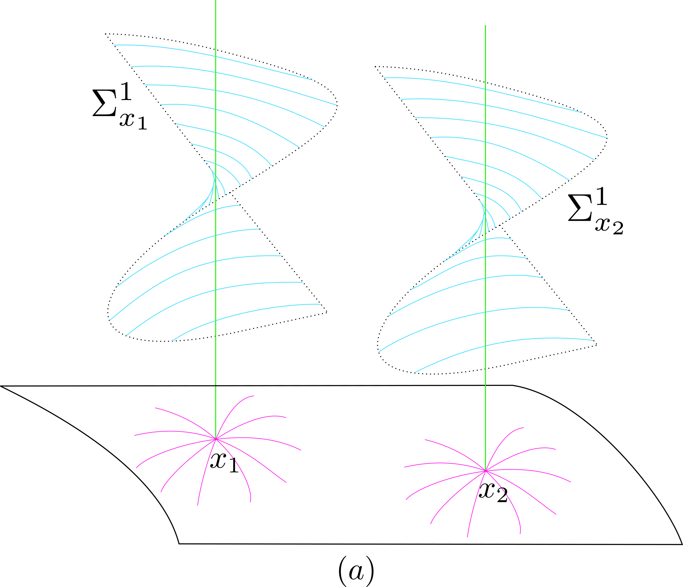
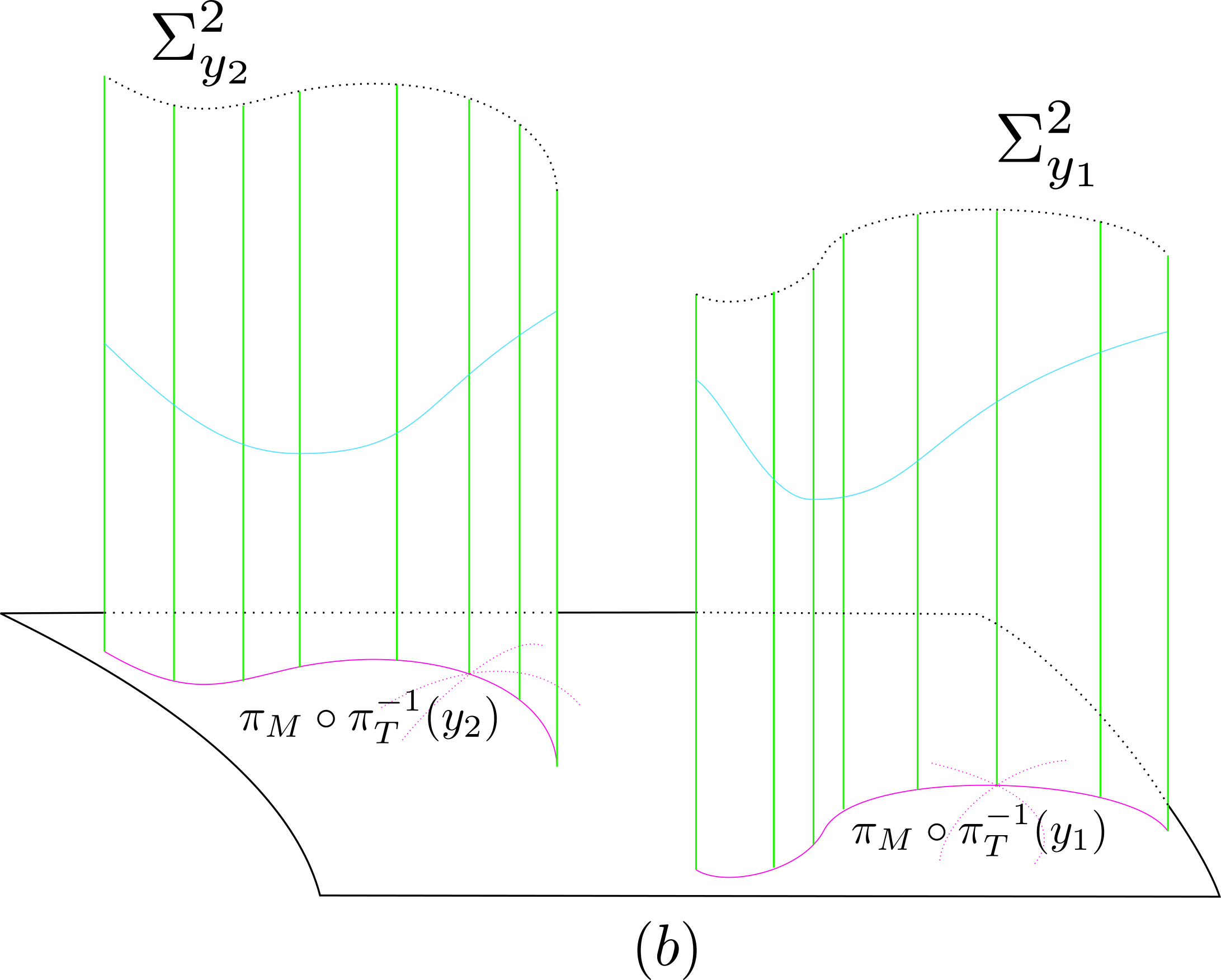
Figure 1. (a) At $x_{1},x_{2}\in M,$ the vertical green lines are open subsets of the fibers $\pi_{M}^{-1}(x_{i})\subset N.$ The blue curves intersecting the fibers $\pi_{M}^{-1}(x_{i})$ are natural lifts of the paths (purple curves) on $M$ passing through $x_{i}.$ The surfaces $\Sigma^{1}_{x_{i}}\subset N$ are foliated by the blue curves and its generating curve is the fiber $\pi_{M}^{-1}(x_{i})$. (b) At $y_{1},y_{2}\in T,$ the solid purple curves on $M$ are the paths $\pi_{M}\circ\pi^{-1}_{T}(y_{i}).$ Their lift to $N,$ represented by solid blue curves, are the generating curves of the ruled surfaces $\Sigma^{2}_{y_{i}}\subset N$ whose ruling lines are vertical green lines which represent open subsets of the fibers $\pi_{M}^{-1}(t)\subset N$ where $t\in\pi_{M}\circ\pi^{-1}_{T}(y_{i}).$

Step 2. We define paths $\gamma_{xy}\subset N$ as intersections of surfaces $\Sigma^{1}_{x},\Sigma^{2}_{y}\subset N$ provided that $(x,y)\in M\times T\setminus N$. Recall from § 2.2 that $N$ is identified with a subset of $M\times T$ comprised of points $(x,y)\in M\times T$ such that $x$ intersects $y$. Hence, any pair of non-intersecting integral curves of $\mathscr{D}_{1}$ and $\mathscr{D}_{2}$ define a path $\gamma_{xy}$.

We shall now show that the collection of all curves $\gamma_{xy}\subset N$ for $(x,y)\in M\times T\setminus N$ define a path geometry on $N$. More precisely, we prove that the set of tangent directions to paths $\gamma_{xy}$ defines an open subset $Q\subset\mathbb{P}TN$ and therefore defines a (generalized) path geometry on $N$.

Proposition 4.1.

Let $(N,\mathscr{D}_{1},\mathscr{D}_{2})$ be a 2-dimensional path geometry on $M:=N/\mathscr{D}_{2}.$ Restricting to a sufficiently small neighborhood $U\subset N$ of any point in $N$ and defining $M_{U}=U/\mathscr{D}_{2}\subset M$ and $T_{U}=U/\mathscr{D}_{1}\subset T,$ one has the following.

• Exactly 1-parameter sub-family of surfaces from $\{\Sigma^{1}_{x}\}_{x\in M_{U}}$ and exactly 1-parameter sub-family of surfaces from $\{\Sigma^{2}_{y}\}_{y\in T_{U}}$ pass through any point of $U$.

• For any two $\Sigma^{1}_{x^{1}}$, $\Sigma^{1}_{x^{2}}$ passing through a fixed point of $U$ their tangent spaces have a common line, namely $\mathscr{D}_{1}$, and similarly, for any two $\Sigma^{2}_{y^{1}}$, $\Sigma^{2}_{y^{2}}$ passing through a fixed point of $U$ their tangent spaces have a common line, namely $\mathscr{D}_{2}$.

• Exactly one surface from the family $\{\Sigma^{1}_{x}\}_{x\in M_{U}}$ is tangent to the contact distribution $\mathscr{C}=\mathscr{D}_{1}\oplus\mathscr{D}_{2}$ and exactly one surface from family $\{\Sigma^{2}_{y}\}_{y\in T_{U}}$ is tangent to $\mathscr{C}$ at each point $p\in U$; any other pair of surfaces from these two families passing through $p$ intersect along a line at $p$.

Proof.

Identify $U$ as a subset of $M_{U}\times T_{U}$ as explained in § 2.2 and fix $p\in U$. Thus, the point $p\in U$ can be represented as a pair $(\hat{x},\hat{y})\in M_{U}\times T_{U}$. Then a surface $\Sigma^{1}_{x}$ passes through $p\in U$ if and only if $(x,\hat{y})\in U\subset M_{U}\times T_{U},$ i.e. the integral curve of $\mathscr{D}_{1}$ represented by $x$ intersects the integral curve of $\mathscr{D}_{2}$ represented by $\hat{y}$. Similarly, $\Sigma^{2}_{y}$ passes through $p\in U$ if and only if $(\hat{x},y)\in U\subset M_{U}\times T_{U}$, i.e. the integral curve of $\mathscr{D}_{2}$ represented by $y$ intersects the integral curve of $\mathscr{D}_{1}$ represented by $\hat{x}$. This proves statement (a). Statement (b) follows from the construction as all $\Sigma^{1}_{x}$ are foliated by integral curves of $\mathscr{D}_{1}$ and all $\Sigma^{2}_{y}$ are foliated by integral curves of $\mathscr{D}_{2}$. Furthermore, in order to prove statement (c) notice that, $\Sigma^{1}_{x}$ is tangent to $\mathscr{C}$ at $p$ if and only if $x=\hat{x}$ and $\Sigma^{2}_{y}$ is tangent to $\mathscr{C}$ at $p$ if and only if $y=\hat{y}$. Finally, the tangent spaces of $\Sigma^{1}_{x^{1}}$ and $\Sigma^{1}_{x^{2}}$, as well as $\Sigma^{2}_{y^{1}}$ and $\Sigma^{2}_{y^{2}}$ do not coincide for sufficiently small $U$ because flows of $\mathscr{D}_{1}$ and $\mathscr{D}_{2}$ do not commute since their is the contact distribution, i.e. $[\mathscr{D}_{1},\mathscr{D}_{2}]=TN$. ∎

By Proposition 4.1 it follows that there is an open subset

$$Q\subset\mathbb{P}TU$$

such that the natural lift of the 4-parameter family of paths $\gamma_{xy}\subset U$, where $x\in M_{U}$ and $y\in T_{U}$, are well-defined curves foliating $Q$ giving rise to a 3D path geometry on $U$. Since our consideration is local, from now on we shall assume $U=N.$ As in § 2.1, we denote the tangent direction to the natural lift of paths $\gamma_{xy}$ foliating $Q$ by $\mathscr{X}\subset TQ$ and denote the vertical tangent bundle of the fibration $Q\to N$ by $\mathscr{V}\subset TQ.$ The paths $\gamma_{xy}$ are referred to as dancing paths.

Definition 4.2.

Given a 2D path geometry $(N,\mathscr{D}_{1},\mathscr{D}_{2})$ on $M=N/\mathscr{D}_{2}$, the 3D path geometry $(Q,\mathscr{X},\mathscr{V})$ defined via steps 1 and 2 above is called its corresponding dancing path geometry.

Remark 4.3.

If a 2D path geometry is presented as a scalar second order ODE (2.3) then $N=J^{1}(\mathbb{R},\mathbb{R})$ and

$$Q=\mathbb{P}(TN\setminus\mathscr{C}),$$

i.e. the curves in the dancing path geometry are tangent to all directions that are transverse to the contact distribution $\mathscr{C}$. Moreover, each surface $\Sigma^{1}_{x}\subset N$ projects onto $M:=J^{0}(\mathbb{R},\mathbb{R})$ and is foliated by the lift of all paths in $M$ passing through $x$. On the other hand, each $\Sigma^{2}_{y}\subset N$ locally can be identified with a subset of $\mathbb{P}TM$ restricted to the curve $\pi_{M}\circ\pi^{-1}_{T}(y)\subset M$ where $y\in T.$

Our next proposition is about the pair of second order ODEs that corresponds to a dancing construction.

Proposition 4.4.

Given a 2D path geometry $(N,\mathscr{D}_{1},\mathscr{D}_{2}),$ let

(4.1) $$z^{\prime\prime}=F(t,z,z^{\prime}),$$

be its corresponding scalar 2nd order ODE via the local identification $N\cong J^{1}(\mathbb{R},\mathbb{R})$. Let $(t,z)$ and $(t,z,p)$ be jet coordinates on $J^{0}(\mathbb{R},\mathbb{R})$ and $J^{1}(\mathbb{R},\mathbb{R})$ with $t$ as the independent variable. The dancing paths define a 3D path geometry on $N$ whose corresponding pair of second order ODE is

(4.2) $$z^{\prime\prime}=F(t,z,z^{\prime}),\quad p^{\prime\prime}=G(t,z,p,z^{\prime},p^{\prime}).$$

for a uniquely determined function $G\colon J^{1}(\mathbb{R},\mathbb{R}^{2})\to\mathbb{R}.$

Proof.

Recall that every solution curve of pairs of ODEs for the dancing construction are contained in a surface $\Sigma^{2}_{y}$ for some $y\in M.$ Moreover, the surfaces $\Sigma_{y}^{2}$ project to solutions of (2.3) on $M.$ As a result, it follows that for such choice of coordinates, the original equation (2.3) on $M$ is contained in the system for the dancing path geometry. Hence, the dancing construction extends the original scalar second order ODE to a pair of second order ODEs. ∎

Remark 4.5.

Analogously, one can replace $M$ in Proposition 4.4 by the twistor space $T:=N/\mathscr{D}_{1}$ and take a dual viewpoint in the sense of § 2.2. Identifying $T$ as $J^{0}(\mathbb{R},\mathbb{R})$ with jet coordinates $(\tilde{t},\tilde{v}),$ let $(\tilde{t},\tilde{z},\tilde{p})$ be the induced jet coordinates on $N\cong J^{1}(\mathbb{R},\mathbb{R})$. Similar reasoning as above shows that the dual equation (2.4) on $T$ shows up in the system of the dancing path geometry written in coordinates $(\tilde{t},\tilde{z},\tilde{p})$. From this viewpoint, the dancing construction extends the dual ODE to a system as well. However, the two equations (the original one and the dual) do not show up in the dancing construction at the same time. Each of them appear only for the particular choices of coordinates. Nevertheless, the dancing construction can be thought of as a geometric pairing of the original ODE and its dual into one system.

Remark 4.6.

By Proposition 4.4 and Remark 4.5 the dancing construction can be interpreted as simultaneous moves of two points (dancers): one on the surface $M$ following the curve $x(t)\subset M$ and one on its twistor surface $T$ following the curve $y(t)\subset T,$ such that both paths belong to the mutually dual path geometries on $M$ and $T.$ By our discussion in § 2.2, the paths $x(t)$ and $y(t)$ correspond to two points $\hat{x}\in T$ and $\hat{y}\in M,$ respectively. The first condition in the dancing construction is that the paths of the dancers do not intersect, i.e. $\hat{x}\notin y(t)$ and $\hat{y}\notin x(t)$ which implies $(\hat{y},\hat{x})\in M\times T\backslash N.$ The dancing path are defined by the condition that $(x(t),y(t))\subset N\subset M\times T,$ i.e. at any $t=t_{0}$ the paths $\widehat{y(t_{0})}:=\pi_{M}\circ\pi_{T}^{-1}(y(t_{0}))\subset M$ and $\widehat{x(t_{0})}:=\pi_{T}\circ\pi_{M}^{-1}(x(t_{0}))\subset T$ satisfy $x(t_{0})\in\widehat{y(t_{0})}$ and $y(t_{0})\in\widehat{x(t_{0})}$. This condition defines a unique dancing path on $N$ for any point $(\hat{y},\hat{x})\in M\times T\backslash N,$ i.e. the 4-parameter family of paths for a 3D path geometry on $N$.

In the flat model $M$ and $T$ are $\mathbb{R}\mathbb{P}^{2}$ and $(\mathbb{R}\mathbb{P}^{2})^{*}$, respectively, and the space of dancing paths is $\mathbb{R}\mathbb{P}^{2}\times(\mathbb{R}\mathbb{P}^{2})^{*}\backslash N,$ where $N$ is the set of incident points, as originally studied in [BHLN18]. As will be discussed later, for the flat path geometry on $\mathbb{R}\mathbb{P}^{2}$ the dancing paths coincide with the chains.

One can obtain relatively explicit formulas for the dancing construction, and, in particular, function $G$ in Proposition 4.4 in terms of a general solution function $\Phi\colon M\times T\to\mathbb{R}$ of a scalar second order ODE. Take local coordinate $(t,z)$ on $M$ and $(a,b)$ on $T.$ The coordinates on $T$ can be interpreted as constants of integration for (2.3), as explained in § 2.2. If we fix $\hat{x}=(\hat{t},\hat{z})\in M$ and $\hat{y}=(\hat{a},\hat{b})\in T$ we get

$$\Sigma^{1}_{\hat{x}}=\{(t,z,a,b)\in M\times T\ |\ \Phi(t,z,a,b)=0,\ \Phi(\hat{t},\hat{z},a,b)=0\}$$

$$\Sigma^{2}_{\hat{y}}=\{(t,z,a,b)\in M\times T\ |\ \Phi(t,z,a,b)=0,\ \Phi(t,z,\hat{a},\hat{b})=0\}$$

as subsets of $M\times T$. Hence, the curves of the dancing path geometry are given by

$$\gamma_{\hat{x}\hat{y}}=\{(t,z,a,b)\in M\times T\ |\ \Phi(t,z,a,b)=0,\ \Phi(\hat{t},\hat{z},a,b)=0,\ \Phi(t,z,\hat{a},\hat{b})=0\}.$$

The formulas for $\Sigma^{1}_{\hat{x}}$ and $\Sigma^{2}_{\hat{y}}$ shows that our construction coincides infinitesimally with the dancing condition of [Dun22, Section 4]. Further, using these expressions one is able to obtain the corresponding pair of second order ODEs. Indeed, differentiating $\Phi(t,z,a,b)=0$, $\Phi(\hat{t},\hat{z},a,b)=0$, and $\Phi(t,z,\hat{a},\hat{b})=0$ with respect to $t$ and eliminating $\hat{t},\hat{z},\hat{a},\hat{b}$ as well as the coordinate $a,$ one can express second order derivatives of $z$ and $b$ in terms of their 1-jets with respect to $t$.

Example 4.7.

[Flat path geometry] If (2.3) is trivial, i.e. $F=0$, then

$$\Phi(t,z,a,b)=z-bt-a$$

and $\gamma_{xy}$ are solutions to

$$z^{\prime\prime}=0,\qquad b^{\prime\prime}=-\frac{2(b^{\prime})^{2}}{z^{\prime}-b}.$$

Note that the pair of ODEs above coincides with (3.14). More generally, by Proposition 4.23, flat path geometries are the only case for which dancing paths and chains coincide.

Example 4.8.

[A self-dual path geometry] Consider the scalar second order (2.3) where $F=\sqrt{z^{\prime}}.$ It can be easily checked that for this scalar ODE the induced 2D path geometry is equivalent to its dual. One obtains

$$\Phi(t,z,a,b)=z-(\tfrac{1}{12}t^{3}+\tfrac{1}{4}bt^{2}+\tfrac{1}{4}b^{2}t+a)$$

and, therefore, $\gamma_{xy}$ are solutions to the pair of second order ODEs

$$\begin{gathered}z^{\prime\prime}=\sqrt{z^{\prime}},\\ b^{\prime\prime}=\tfrac{1}{-b^{\prime}(4z^{\prime}-(t+b)^{2})}\left(-2(b^{\prime})^{2}(b^{\prime}+1)^{2}(t+b)+4\sqrt{z^{\prime}}(b^{\prime})^{2}+2(b^{\prime})^{3}\sqrt{(t+b)^{2}b^{\prime}(b^{\prime}+1)-4z^{\prime}b^{\prime}}\right).\end{gathered}$$

Remark 4.9.

Comparing the relation between the ODEs in Proposition 4.4 to the case of chains, in the dancing construction it appears to be much more difficult to give a closed form of the pair of ODEs, unlike the pair (3.13) for chains. An underlying reason is that, as is mentioned in Remark 4.26, 3D path geometry of chains is variational in a canonical way, unlike the path geometry defined by the dancing construction. The variationality of chains, as mentioned in § 3.2, was key in the derivation of the pair of ODEs (3.13).

4.2. Characterization of the dancing construction

In this section we provide a characterization of 3D path geometries obtained via the dancing construction.

Proposition 4.10.

Let $(N,\mathscr{D}_{1},\mathscr{D}_{2})$ be a 2D path geometry on $M:=N/\mathscr{D}_{2}$ with dual path geometry on $T=N/\mathscr{D}_{1}$. Then all surfaces $\Sigma^{1}_{x},\Sigma^{2}_{y}\subset N$, $x\in M$ and $y\in T$ are totally geodesic in the dancing construction, i.e. if a path is tangent to $\Sigma^{1}_{x}$ or $\Sigma^{2}_{y}$ at a point, then it stays in $\Sigma^{1}_{x}$ or $\Sigma^{2}_{y}$, respectively.

Proof.

This is a direct consequence of the constructions because all paths tangent to $\Sigma^{1}_{x}$ are of the form $\Sigma^{1}_{x}\cap\Sigma^{2}_{y}$, for some $y\in T$. Similarly, all paths tangent to $\Sigma^{2}_{y}$ are of the form $\Sigma^{2}_{y}\cap\Sigma^{1}_{x}$ for some $x\in M$. ∎

It follows from Proposition 4.10 that surfaces $\Sigma^{1}_{x}$ and $\Sigma^{2}_{y}$ for all $x\in M$ and $y\in T$ are equipped with their own 2D path geometries. Hence, we arrive at the following proposition.

Proposition 4.11.

Let $(N,\mathscr{D}_{1},\mathscr{D}_{2})$ be a 2D path geometry on $M:=N/\mathscr{D}_{2}$ with dual path geometry on $T:=N/\mathscr{D}_{1}.$ For any $x\in M$, the restriction of the projection $\pi_{M}\colon N\to M$ to $\Sigma^{1}_{x}$ establishes the equivalence of path geometries on $\Sigma^{2}_{y}$ and $M$. Similarly, for any $y\in T$ the restriction of the projection $\pi_{T}\colon N\to T$ to $\Sigma^{2}_{y}$ establishes the equivalence of path geometries on $\Sigma^{1}_{x}$ and $T$.

Proof.

Fix $x\in M$ and the corresponding surface $\Sigma^{1}_{x}$. The path geometry on $\Sigma^{1}_{x}$ is defined by intersections of $\Sigma^{1}_{x}$ with all surfaces $\Sigma^{2}_{y}\subset N$, $y\in T$. The image of $\Sigma^{2}_{y}$ under the projection $\pi_{M}$ is a path on $M$ corresponding to $y\in T$. Therefore the dancing path $\gamma_{xy}:=\Sigma^{1}_{x}\cap\Sigma^{2}_{y}$ is projected to a path for the original path geometry on $M$. Second part of the proposition is shown analogously. ∎

Now, we are ready to state our characterization of dancing path geometries.

Theorem 4.12.

Let $(Q,\mathscr{X},\mathscr{V})$ be a 3D path geometry on $N:=Q/\mathscr{V}.$ Then $(Q,\mathscr{X},\mathscr{V})$ is a dancing path geometry if and only if there are two 2-parameter families $\{\Sigma^{1}_{x}\}_{x\in\tilde{M}}$ and $\{\Sigma^{2}_{y}\}_{y\in\tilde{T}}$ of totally geodesic surfaces in $N$ with the following properties.

• Exactly 1-parameter sub-family of surfaces from $\{\Sigma^{1}_{x}\}_{x\in\tilde{M}}$ and exactly 1-parameter sub-family of surfaces from $\{\Sigma^{2}_{y}\}_{y\in\tilde{T}}$ pass through any point of $N$.

• Tangent planes to all surfaces $\Sigma^{1}_{x}$ (respectively, $\Sigma^{2}_{y})$ which pass through a fixed point of $N$ have a common line denoted as $\mathscr{D}_{1}$ (respectively, $\mathscr{D}_{2}.$)

• The rank 2 distribution $\mathscr{C}:=\mathscr{D}_{1}\oplus\mathscr{D}_{2}\subset TN$ is contact.

• Path geometries on all surfaces $\Sigma^{1}_{x}$, $x\in\tilde{M}$, are equivalent to the 2D path geometry induced on $N/\mathscr{D}_{2}$ whose paths are the projection of the integral curves of $\mathscr{D}_{1}.$ Moreover, path geometries on all surfaces $\Sigma^{2}_{y}$, $y\in\tilde{T}$, are equivalent to the 2D path geometry induced on $N/\mathscr{D}_{1}$ whose paths are the projection of $\mathscr{D}_{2}.$

Proof.

If a path geometry comes from the dancing construction then $\tilde{T}=T:=N/\mathscr{D}_{1}$ and $\tilde{M}=M:=N/\mathscr{D}_{2}$ and the conditions (a)-(c) are satisfied by definition (see Proposition 4.1). Furthermore, the surfaces $\Sigma^{1}_{x}$ and $\Sigma^{2}_{y}$ are totally geodesic due to Proposition 4.10 and condition (d) is satisfied by Proposition 4.11.

On the other hand, if conditions (a)-(c) are satisfied then the pair $(\mathscr{D}_{1},\mathscr{D}_{2})$ is a 2D path geometry on $N$ by (b) and (c). The claim follows if we prove that surfaces $\Sigma^{1}_{x}$ and $\Sigma^{2}_{y}$ are necessarily obtained via the dancing construction applied to $(\mathscr{D}_{1},\mathscr{D}_{2})$. First we prove that $\Sigma^{1}_{x}\cap\Sigma^{2}_{y}$ is a path of the original 3D path geometry for all $x$ and $y$. Indeed, since both $\Sigma^{1}_{x}$ and $\Sigma^{2}_{y}$ are totally geodesic, any path tangent to $\Sigma^{1}_{x}$ and $\Sigma^{2}_{y}$ at some point has to stay simultaneously in both $\Sigma^{1}_{x}$ and $\Sigma^{2}_{y}$ at all time. Hence, the path coincides with $\Sigma^{1}_{x}\cap\Sigma^{2}_{y}$.

Furthermore, by condition (b) any surface $\Sigma^{1}_{x}$ is foliated by integral curves of $\mathscr{D}_{1}.$ Hence, the projection of $\Sigma^{1}_{x}$ to $N/\mathscr{D}_{1}$ is a curve. By (d), this curve is necessarily a projection of an integral curve of $\mathscr{D}_{2}$, i.e. $\Sigma^{1}_{x}$ is defined as the union of integral curves of $\mathscr{D}_{2}$ crossing a choice of integral curve of $\mathscr{D}_{1}$. In this way we identify $\tilde{T}$ with $N/\mathscr{D}_{1}$. Similarly, we prove that $\tilde{M}$ can be identified with $N/\mathscr{D}_{2}$ and that any $\Sigma^{2}_{y}$ is defined as a union of integral curves of $\mathscr{D}_{1}$ crossing a choice of integral curve of $\mathscr{D}_{2}$.

∎

4.3. Freestyling: a generalization of dancing

Theorem 4.12 suggests that one can consider a generalization of dancing path geometries by dropping condition (d). Later on we shall provide equivalent descriptions.

Definition 4.13.

A 3D path geometry $(Q,\mathscr{X},\mathscr{V})$ on $N:=Q/\mathscr{V}$ is a freestyling if it admits two 2-parameter families $\{\Sigma^{1}_{x}\}_{x\in\tilde{M}}$ and $\{\Sigma^{2}_{y}\}_{y\in\tilde{T}}$ of totally geodesic surfaces in $N$ with the following properties.

• Exactly 1-parameter sub-family of surfaces from $\{\Sigma^{1}_{x}\}_{x\in\tilde{M}}$ and exactly 1-parameter sub-family of surfaces from $\{\Sigma^{2}_{y}\}_{y\in\tilde{T}}$ pass through any point of $N$.

• Tangent planes to all surfaces $\Sigma^{1}_{x}$ (respectively, $\Sigma^{2}_{y})$ which pass through a fixed point of $N$ have a common line denoted as $\mathscr{D}_{1}$ (respectively, $\mathscr{D}_{2}.$)

• The rank 2 distribution $\mathscr{C}:=\mathscr{D}_{1}\oplus\mathscr{D}_{2}\subset TN$ is contact.

Now we have the following.

Proposition 4.14.

Any freestyling on a 3-dimensional manifold $N$ with a contact distribution $\mathscr{C}\subset TN$ uniquely determines, in sufficiently small open sets, a triple of 2D path geometries $(N,\mathscr{D}_{1},\mathscr{D}_{2})$, $(N,\tilde{\mathscr{D}}_{1},\mathscr{D}_{2})$, $(N,\mathscr{D}_{1},\tilde{\mathscr{D}}_{2})$ such that $\mathscr{C}=\mathscr{D}_{1}\oplus\mathscr{D}_{2}=\tilde{\mathscr{D}}_{1}\oplus\mathscr{D}_{2}=\mathscr{D}_{1}\oplus\tilde{\mathscr{D}}_{2}.$

Proof.

By condition (c) in Definition 4.13, a freestyling path geometry defines a 2D path geometry $(N,\mathscr{D}_{1},\mathscr{D}_{2})$ on $M:=N/\mathscr{D}_{2}.$ Furthermore, $N$ is equipped with two additional families of surfaces $\{\Sigma^{1}_{x}\}_{x\in\tilde{M}}$ and $\{\Sigma^{2}_{y}\}_{y\in\tilde{T}}$. For general freestyling $\tilde{M}$ and $\tilde{T}$ cannot be identified with $M:=N/\mathscr{D}_{2}$ and $T:=N/\mathscr{D}_{1}$, respectively. However, by conditions (a) and (b), for any $x\in\tilde{M}$, $\Sigma^{1}_{x}$ is foliated by integral curves of $\mathscr{D}_{2}$, and for any $y\in\tilde{T}$, $\Sigma^{2}_{y}$ is foliated by integral curves of $\mathscr{D}_{1}$. It follows that $\pi_{T}(\Sigma^{1}_{x})$ and $\pi_{M}(\Sigma^{2}_{y})$ are well-defined curves in the quotient spaces $M=N/\mathscr{D}_{2}$ and $T=N/\mathscr{D}_{2},$ respectively. The 2-parameter family of curves $\{\pi_{T}(\Sigma^{1}_{x})\}_{x\in\tilde{M}}$ defines an additional path geometry on $T$ and the family $\{\pi_{M}(\Sigma^{2}_{y})\}_{y\in\tilde{T}}$ defines an additional path geometry on $M$. Note that in this regard $\tilde{T}$ and $\tilde{M}$ become the twistor spaces for the path geometry on $M$ and $T$, respectively. To show the last part of the proposition, one notes that, in sufficiently small open sets, $N$ can be identified as $\mathbb{P}TM,$ where $M=N/\mathscr{D}_{2},$ with canonical contact distribution $\mathscr{C}$ splitting as $\mathscr{C}=\mathscr{D}_{1}\oplus\mathscr{D}_{2}=\tilde{\mathscr{D}}_{1}\oplus\mathscr{D}_{2}.$ Viewing $N$ as $\mathbb{P}T(N/\mathscr{D}_{1}),$ in sufficiently small neighborhoods, it follows that $\mathscr{C}=\mathscr{D}_{1}\oplus\mathscr{D}_{2}=\mathscr{D}_{1}\oplus\tilde{\mathscr{D}}_{2}.$ ∎

Remark 4.15.

In the case of the usual dancing construction one has $\tilde{\mathscr{D}}_{1}=\mathscr{D}_{1}$ and $\tilde{\mathscr{D}}_{2}=\mathscr{D}_{2}$. Now, having three 2D path geometries $(N,\mathscr{D}_{1},\mathscr{D}_{2})$, $(N,\tilde{\mathscr{D}}_{1},\mathscr{D}_{2})$, $(N,\mathscr{D}_{1},\tilde{\mathscr{D}}_{2}),$ we can repeat what we did in the case of the dancing construction, but use the pair of line fields $(\mathscr{D}_{1},\tilde{\mathscr{D}}_{2})$ and $(\tilde{\mathscr{D}}_{1},\mathscr{D}_{2})$ in order to define $\Sigma^{1}_{x}$ and $\Sigma^{2}_{y},$ respectively. According to Proposition 4.14, this gives rise to a freestyling path geometry. Moreover, it follows that Proposition 4.11 can be extended for freestyling in the sense that the 2D path geometries induced on $\tilde{M}$ and $\tilde{T}$ are equivalent to the induced 2D path geometries on any of the surfaces $\Sigma^{2}_{y}$ and $\Sigma^{1}_{x},$ respectively.

Remark 4.16.

Similarly to Remark 4.6, one can express the pair of second order ODEs that corresponds to a freestyling. In this case the starting point would be three functions $\Phi_{1}\colon M\times T\to\mathbb{R}$, $\Phi_{2}\colon M\times\tilde{T}\to\mathbb{R}$, and $\Phi_{3}\colon\tilde{M}\times T\to\mathbb{R}$, where $\tilde{T}=N/\tilde{\mathscr{D}}_{1}$ and $\tilde{M}=N/\tilde{\mathscr{D}}_{2}$ are two additional leaf spaces related to two additional path geometries $(N,\tilde{\mathscr{D}}_{1},\mathscr{D}_{2})$ and $(N,\mathscr{D}_{1},\tilde{\mathscr{D}}_{2})$. Clearly, $N$ is identified simultaneously with subsets $\{\Phi_{1}=0\}$, $\{\Phi_{2}=0\}$, and $\{\Phi_{3}=0\}$ of $M\times T$, $M\times\tilde{T}$ and $\tilde{M}\times T$, respectively.

Let us use $(t,z)$ and $(\hat{t},\hat{z})$ as coordinates on $M$ and $\tilde{M},$ respectively, and $(a,b)$ and $(\hat{a},\hat{b})$ as coordinates on $T$ and $\tilde{T},$ respectively. It follows that

$$\Sigma^{1}_{\hat{x}}=\{(t,z,a,b)\in M\times T\ |\ \Phi_{1}(t,z,a,b)=0,\ \Phi_{3}(\hat{t},\hat{z},a,b)=0\},$$

$$\Sigma^{2}_{\hat{y}}=\{(t,z,a,b)\in M\times T\ |\ \Phi_{1}(t,z,a,b)=0,\ \Phi_{2}(t,z,\hat{a},\hat{b})=0\},$$

where $\hat{x}=(\hat{t},\hat{z})$ is a fixed point in $\tilde{M}$ and $\hat{y}=(\hat{a},\hat{b})$ is a fixed point in $\tilde{T}$. Consequently, one obtains

$$\gamma_{\hat{x}\hat{y}}=\{(t,z,a,b)\in M\times T\ |\ \Phi_{1}(t,z,a,b)=0,\ \Phi_{3}(\hat{t},\hat{z},a,b)=0,\ \Phi_{2}(t,z,\hat{a},\hat{b})=0\}$$

are paths for the freestyling.

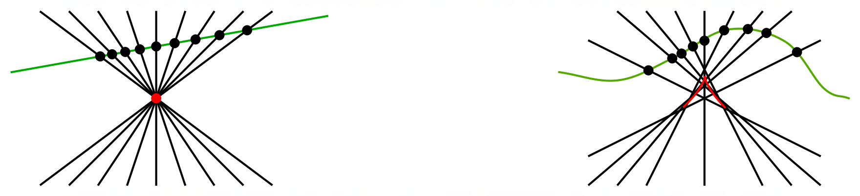
Figure 2. A visualization of the dancing paths on the left, and of the freestyling on the right, viewed through the geometry on $M$. Points in $N$ are represented by black lines with distinguished points. A dancing path in $N$ is uniquely defined by a green line and a red point that doesn’t lie on this line. The line and the point are projections of nonintersecting integral curves of $\mathscr{D}_{1}$ (green line) and of $\mathscr{D}_{2}$ (a red point). A dancing path consists of lines passing through the red point with marked points defined as intersection points with the green line. In the freestyling a green line is replaced by a curve from the additional path geometry on $M$. Similarly, instead of the family of lines passing through the red point we have a 1-parameter family parameterized by a curve from the additional path geometry on $T$ (whose projection to $M$ is no longer a point in $M$ but a red cusp).

Example 4.17.

Consider a freestyling defined by three 2D path geometries such that two of them, namely $(N,\mathscr{D}_{1},\mathscr{D}_{2})$ and $(N,\mathscr{D}_{1},\tilde{\mathscr{D}}_{2}),$ are flat, but the third one $(N,\tilde{\mathscr{D}}_{1},\mathscr{D}_{2})$ is arbitrary, defined by a general second order ODE $z^{\prime\prime}=F(t,z,z^{\prime})$. We have

$$\Phi_{1}(t,z,a,b)=z-at-b,\qquad\Phi_{3}(\hat{t},\hat{z},a,b)=\hat{z}-b\hat{t}-a.$$

On the other hand, by definition, the solution function $\Phi_{2}=\Phi(t,z,\hat{a},\hat{b})$ for $(N,\tilde{\mathscr{D}}_{1},\mathscr{D}_{2})$ is a function such that differentiating $\Phi_{2}$ twice with respect to $t$ and expressing constants of integration $(\hat{a},\hat{b})$ with respect to $t,z,z^{\prime}$ one gets $z^{\prime\prime}=F(t,z,z^{\prime})$. Now, assuming $a$ and $b$ are functions of $t$ and differentiating $\Phi_{3}$ with respect to $t$, we express constants $(\hat{t},\hat{z})$ as

$$\hat{t}=-\tfrac{a^{\prime}}{b^{\prime}},\qquad\hat{z}=a-b\tfrac{a^{\prime}}{b^{\prime}}$$

One more differentiation of $\Phi_{3}$ gives

(4.3) $$b^{\prime\prime}=a^{\prime\prime}\tfrac{a^{\prime}}{b^{\prime}}.$$

Differentiating $\Phi_{1}$ with respect to $t$ and exploiting $z^{\prime\prime}=F(t,z,z^{\prime}),$ we are able to compute $a$, $a^{\prime}$ and $a^{\prime\prime}$ in terms of $t$, $z$ and $b$ and their derivatives with respect to $t$. Consequently, we get

(4.4) $$a^{\prime}=z^{\prime}-b^{\prime}t-b,\qquad a^{\prime\prime}=F(t,z,z^{\prime})-b^{\prime\prime}t-2b^{\prime}.$$

Combining (4.3) with (4.4) we get $b^{\prime\prime}=\frac{(F-2b^{\prime})b^{\prime}}{z^{\prime}-b}$. Summarizing, the 3D freestyling path geometry is described by the system

$$z^{\prime\prime}=F(t,z,z^{\prime}),\qquad b^{\prime\prime}=\tfrac{b^{\prime}}{z^{\prime}-b}\left(F(t,z,z^{\prime})-2b^{\prime}\right).$$

4.4. 3D path geometries arising from dancing and freestyling

Let $(Q,\mathscr{V},\mathscr{X})$ be a 3D path geometry on $N:=Q/\mathscr{V}$. In this section our objective is to characterize those triples $(Q,\mathscr{V},\mathscr{X})$ that define a freestyling by exploiting Theorem 2.4. Thus, we need to interpret the properties of Definition 4.13, expressed at the level of the 3-dimensional manifold $N$, on the 5-dimensional manifold $Q$.

Theorem 4.18.

Let $(Q,\mathscr{V},\mathscr{X})$ be a 3D path geometry on $N=Q/\mathscr{V}.$ Then $(Q,\mathscr{V},\mathscr{X})$ is freestyling if and only if the vertical bundle $\mathscr{V}$ has a splitting $\mathscr{V}=\mathscr{V}_{1}\oplus\mathscr{V}_{2}$ with the following properties.

• The distributions

  $$\mathscr{B}_{1}=\operatorname{span}\{\mathscr{V}_{1},\mathscr{X},[\mathscr{V}_{1},\mathscr{X}]\},\qquad\mathscr{B}_{2}=\operatorname{span}\{\mathscr{V}_{2},\mathscr{X},[\mathscr{V}_{2},\mathscr{X}]\}$$

  are integrable.

• Rank 3 distributions $\mathscr{B}_{1}$ and $\mathscr{B}_{2}$ have rank-2 sub-distributions $\tilde{\mathscr{K}}_{1}$ and $\tilde{\mathscr{K}}_{2}$ containing $\mathscr{V}_{1}$ and $\mathscr{V}_{2}$, respectively, such that rank 3 distributions

  $$\mathscr{K}_{1}=\tilde{\mathscr{K}}_{1}\oplus\mathscr{V}_{2}\qquad\mathscr{K}_{2}=\tilde{\mathscr{K}}_{2}\oplus\mathscr{V}_{1}$$

  are integrable.

• The projections of $\mathscr{K}_{1}$ and $\mathscr{K}_{2}$ to $N$ span a contact distribution.

Proof.

Surfaces $\Sigma^{1}_{x},x\in M,$ and $\Sigma^{2}_{y},y\in T,$ are the projection of the leaves of $\mathscr{B}_{2}$ and $\mathscr{B}_{1}$ to $N$. Then, by (b), distributions $\mathscr{K}_{1}$ and $\mathscr{K}_{2}$ project to line fields $\mathscr{D}_{1}$ and $\mathscr{D}_{2}$ on $N,$ respectively. The only nontrivial observation needed here is that condition (a) implies that any leaf of $\mathscr{B}_{1}$ or $\mathscr{B}_{2}$ project to a totally geodesic surface in $N$. This follows from the fact that the paths of the 3D path geometry are defined as projections of integral curves of $\mathscr{X}$ to $N$. Since $\mathscr{B}_{1}$ and $\mathscr{B}_{2}$ are integrable, the paths that are tangent to the surface at a point stay in the surface. ∎

Remark 4.19.

We point out that the three parts of Theorem 4.18 can provide an alternative definition of freestyling instead of the one given in Definition 4.13. Moreover, following [KM21, Section 4.2], one can show that condition (1) in the theorem above implies that $\mathscr{V}_{1}$ and $\mathscr{V}_{2}$ are eigenspaces of the torsion of the 3D path geometry viewed as a trace-free $2\times 2$-matrix acting on $\mathscr{V}.$

Proposition 4.20.

Any freestyling defines a principal $B$-subbundle $\iota\colon\mathcal{G}_{T_{G_{r}}}\hookrightarrow\mathcal{G},$ where $B\subset\mathrm{GL}(2,\mathbb{R})$ is the Borel subgroup, over which the following invariant conditions are satisfied.

$$\iota^{*}A_{0}=\iota^{*}A_{2}=0,\quad\iota^{*}W_{2}=\pm 1,$$

and the components of $\iota^{*}\psi$, as given in (2.5), satisfy

$$\iota^{*}\psi^{1}_{2}\equiv 0 \mod\{\iota^{*}\alpha^{0},\iota^{*}\alpha^{2},\iota^{*}\beta^{2}\},$$

$$\iota^{*}\psi^{2}_{1}\equiv 0 \mod\{\iota^{*}\alpha^{0},\iota^{*}\alpha^{1},\iota^{*}\beta^{1}\},$$

$$\iota^{*}\psi^{2}_{2}\equiv -\iota^{*}\psi^{1}_{1} \mod\{\iota^{*}\alpha^{0},\iota^{*}\alpha^{1},\iota^{*}\alpha^{2}\}$$

$$\iota^{*}\nu_{1},\iota^{*}\mu_{1},\iota^{*}\nu_{2},\iota^{*}\mu_{2}\equiv 0 \mod\{\iota^{*}\alpha^{0},\iota^{*}\alpha^{1},\iota^{*}\alpha^{2},\iota^{*}\beta^{1},\iota^{*}\beta^{2}\}$$

As a result, given a freestyling path geometry $(\mathcal{G}\to Q,\psi)$, its curvature has at least two distinct real roots whose multiplicities are at most two and its torsion is either zero or has two distinct real roots.

Proof.

By Theorem 4.18, a freestyling gives a splitting $\mathscr{V}=\mathscr{V}_{1}\oplus\mathscr{V}_{2}.$ Since the structure group of a 3D path geometry is $P_{0}=\mathbb{R}^{*}\times\mathrm{GL}(2,\mathbb{R}),$ having a splitting reduced $P_{0}$ to $(\mathbb{R}^{*})^{3}$ in order for the splitting to be preserved. Thus, similarly to Proposition 3.9, such a splitting gives an inclusion $\iota_{1}\colon\mathcal{G}^{(1)}\to\mathcal{G},$ where $\mathcal{G}^{(1)}$ is a principal $P^{(1)}$-bundle with $P^{(1)}:=(\mathbb{R}^{*})^{3}\ltimes P_{+}$ over which

(4.5) $$\iota_{1}^{*}\psi^{1}_{2}=A^{1}_{2i}\alpha^{i}+B^{1}_{2a}\beta^{a},\quad\iota_{1}^{*}\psi^{2}_{1}=A^{2}_{1i}\alpha^{i}+B^{2}_{1a}\beta^{a}$$

for some functions $A^{a}_{bi}$ and $B^{a}_{bc}$ on $\mathcal{G}^{(1)}.$ In terms of the Cartan connection (2.5) one has $\mathscr{V}_{a}=\langle\tfrac{\partial}{\partial s^{*}\beta^{a}}\rangle$ and $\mathscr{X}=\langle\tfrac{\partial}{\partial s^{*}\alpha^{0}}\rangle$ for any section $s\colon Q\to\mathcal{G}^{(1)}.$ This implies that $[\mathscr{X},\mathscr{V}_{a}]=\langle\tfrac{\partial}{\partial s^{*}\alpha^{a}}\rangle.$ As a result, for the rank 3 integrable distributions in 4.18 one has $\mathscr{B}_{a}=\ker\mathcal{I}_{a}$ where $\mathcal{I}_{1}:=\{\alpha^{2},\beta^{2}\}$ and $\mathcal{I}_{2}:=\{\alpha^{1},\beta^{1}\}.$ Using the structure equations, one immediately obtains, in case the torsion $\mathbf{T}$ is nonzero, that the integrability of $\iota_{1}^{*}\mathcal{I}_{1}$ and $\iota_{1}^{*}\mathcal{I}_{2}$ implies

(4.6) $$\iota_{1}^{*}A_{0}=0,\quad\iota_{1}^{*}A_{2}=0.$$

Moreover, as a result of differential relations arising from the integrability of $\iota_{1}^{*}\mathcal{I}_{1}$ and $\iota_{1}^{*}\mathcal{I}_{2},$ it follows that

(4.7) $$\iota_{1}^{*}W_{0}=0,\quad\iota^{*}_{1}W_{4}=0.$$

By part (b) of Theorem 4.18 the integrability of $\mathscr{K}_{1}$ and $\mathscr{K}_{2}$ are required for freestyling. In order to impose these integrability conditions, as in Proposition 3.9, an additional reduction to a principal $P^{(2)}$-bundle $\iota_{2}\colon\mathcal{G}^{(2)}\hookrightarrow\mathcal{G}^{(1)}$ is required where $P^{(2)}\cong(\mathbb{R}^{*})^{3}\ltimes\mathbb{R}$ and

(4.8) $$\mathcal{G}^{(2)}=\{u\in\mathcal{G}^{(1)}\ \vline\ B^{1}_{21}(u)=B^{2}_{12}(u)=A^{1}_{21}(u)=A^{2}_{12}(u)=0\}.$$

As in Proposition 3.9, one has $\iota_{2}^{*}\mu_{1},\iota_{2}^{*}\mu_{2},\iota_{2}^{*}\nu_{1},\iota_{2}^{*}\nu_{2}$ are zero modulo $\{\iota^{*}_{2}\alpha^{0},\iota^{*}_{2}\alpha^{1},\iota^{*}_{2}\alpha^{2},\iota^{*}_{2}\beta^{1},\iota^{*}_{2}\beta^{2}\}.$ As a result, the integrability of $\mathcal{I}_{3}=\mathrm{Ann}\mathscr{K}_{1}$ and $\mathcal{I}_{4}=\mathrm{Ann}\mathscr{K}_{2}$ on $\mathcal{G}^{(2)}$ is well-defined. It is matter of straightforward computation to show that if $\mathcal{I}_{3}$ and $\mathcal{I}_{4}$ are integrable on $\mathcal{G}^{(2)}$ then

$$\mathrm{d}\alpha^{0}\equiv W_{2}\alpha^{1}{\,{\wedge}\;}\alpha^{2}\mod\{\alpha^{0}\},$$

wherein we have suppressed the pull-backs. As a result, condition (c) in Theorem 4.18 implies that for a freestyling

(4.9) $$\iota_{2}^{*}W_{2}\neq 0$$

which combined with (4.6) and (4.7) shows that the quartic $\mathbf{C}$ has at least two real roots whose multiplicity is at most two.

Lastly, using (4.9), there is a third reduction of the structure bundle to a principal $P^{(3)}$-bundle $\iota_{3}\colon\mathcal{G}^{(3)}\hookrightarrow\mathcal{G}^{(2)}$ where $P^{(3)}=(\mathbb{R}^{*})^{2}\ltimes\mathbb{R}\cong B,$ where $B\subset\mathrm{GL}(2,\mathbb{R})$ is the Borel subgroup, defined as

(4.10) $$\mathcal{G}^{(3)}=\{u\in\mathcal{G}^{(2)}\ \vline\ W_{2}(u)=1\}.$$

where we have assumed $W_{2}(u)>0$ (see Remark 3.14 for a discussion on the sign of $W_{2}$ which remains equally valid here as well.) On $\mathcal{G}^{(3)}$ one obtains that $\iota^{*}_{3}(\psi^{2}_{2}+\psi^{1}_{1})$ is semi-basic with respect to the fibration $\mathcal{G}^{(3)}\to Q.$ This finishes the proof where $\mathcal{G}_{T_{G_{r}}}:=\mathcal{G}^{(3)}$ and $B=(\mathbb{R}^{*})^{2}\ltimes\mathbb{R}$ and $\iota:=\iota_{3}\circ\iota_{2}\circ\iota_{1}.$ The full structure equations for the $\{e\}$-structures $\iota^{*}\psi$ on $\mathcal{G}_{T_{G_{r}}}$ is given in (A.2) for some quantities $x_{i}$’s on $\mathcal{G}_{T_{G_{r}}}$ where

$$\iota^{*}\psi^{2}_{2}=-\iota^{*}\psi^{1}_{1}+4\iota^{*}x_{15}\alpha^{0}+4\iota^{*}x_{11}\alpha^{1}-4\iota^{*}x_{12}\alpha^{2}.$$

∎

Remark 4.21.

We point out that in $\mathcal{G}_{T_{G_{r}}}$ the subscript $T_{G_{r}}$ is chosen to point out that the algebraic type of the torsion $\mathbf{T},$ represented as the quadric (2.11), is general with two real roots, in analogy with the subscript $D_{r}$ in $\mathcal{G}_{D_{r}}$ mentioned in Remark 3.10. Moreover, in comparison with Proposition 3.9, the same reductions were carried out in the proposition above although in a different order. Since the proof is almost identical to that of Proposition 3.9, we skipped some of the details. We point out that, unlike Proposition 3.9, the principal $B$-bundle $(\mathcal{G}_{T_{G_{r}}}\to Q,\iota^{*}\psi)$ does not define a Cartan geometry, as can be seen from the non-horizontal 2-forms in the structure equations for $\mathrm{d}\mu_{0}$ in (A.2). However the principal $\mathbb{R}^{*}\times B$-bundle $(\mathcal{G}^{(2)}\to Q,(\iota_{2}\circ\iota_{1})^{*}\psi)$ does define a Cartan geometry. This is due to the fact that the third reduction involving the normalization of $W_{2}$ to $\pm 1$ breaks the equivariancy. It is a matter of straightforward computation to show that if one requires such structures to define a Cartan connection, i.e. $x_{11}=x_{12}=x_{15}=0$ then the freestyling is torsion-free, which is the case treated in Proposition 4.23.

Remark 4.22.

Another outcome of Proposition 4.20 is that projection of the paths of any freestyling to $N$ is always transverse to the contact distribution. This is due to the fact that the path are tangent to the line field spanned by $\tfrac{\partial}{\partial\alpha^{0}}$ and that $\alpha^{0}$ is a contact form on $N.$ Lastly, in the language of [MS23], $(\mathcal{G}^{(2)}\to Q,(\iota_{2}\circ\iota_{1})^{*}\psi)$ defines an orthopath geometry since the 2-form $\alpha^{1}{\,{\wedge}\;}\beta^{2}+\alpha^{2}{\,{\wedge}\;}\beta^{1}\in\Omega^{2}(\mathcal{G}^{(2)})$ is well-defined which also satisfies

$$\mathrm{d}\rho=-2(\psi^{1}_{1}+\psi^{2}_{2}){\,{\wedge}\;}\rho+A_{1}\alpha^{0}{\,{\wedge}\;}\alpha^{1}{\,{\wedge}\;}\alpha^{2}.$$

As a result, such structures define an variational orthopath geometry, i.e. $\mathrm{d}\rho\equiv 0$ modulo $\{\rho\}$ if and only if they are torsion-free which is treated in the next proposition.

As mentioned in the two remarks above, torsion-free freestyling is very special.

Proposition 4.23.

The following are equivalent.

1. The torsion of a freestyling is zero.

2. The curvature of a freestyling has two distinct real roots of multiplicity two.

3. A freestyling is locally equivalent to the chains of the flat 2D path geometry.

Proof.

Let us show $(1)\to(2):$ Using the $\{e\}$-structure obtained in Proposition 4.20 and the structure equations (A.2), it follows that there is only one fundamental invariant. Moreover, one obtains differential relations

(4.11) $$W_{3}=-\tfrac{1}{6}A_{1;\underline{2221}},\quad W_{1}=\tfrac{1}{6}A_{1;\underline{1112}}.$$

Thus, $A_{1}=0$ implies $W_{1}=W_{3}=0,$ which combined with $W_{0}=W_{4}=0$ from (4.7), gives (2).

To show $(2)\to(1)$ we note that the conditions $W_{1}=W_{3}=0$ are invariantly defined on $\mathcal{G}_{T_{G_{r}}}.$ Assuming $W_{1}=W_{3}=0$, it is a matter of tedious but straightforward calculations to show that the identities arising from $\mathrm{d}^{2}=0$ and their resulting differential consequences (in fact three iterations are needed) imply $A_{1}=0.$

Showing $(1)\leftrightarrow(3)$ is a straightforward computation as shown in Proposition 3.9 and Theorem 3.12. Starting from (1), since it implies the curvature has two distinct real roots of multiplicity 2, one can check all the necessary and sufficient conditions are satisfied and the claim follows. Conversely, starting from the chains of the flat 2D path geometry, by the discussion in § 3.1 one can easily check that the conditions in Theorem 4.18 are satisfied on $\mathcal{G}_{D_{r}}$ and moreover $\mathbf{T}=0$ for such freestyling. ∎

Remark 4.24.

The proposition above generalizes the result in [Dun22, Theorem 2.3] where it is shown that a dancing path geometry is torsion-free if and only if it corresponds to the chains of the flat 2D path geometry. Moreover, from Propositions 4.20 and 4.23 it follows that in the $\{e\}$-structure $(\mathcal{G}_{T_{G_{r}}}\to Q,\iota^{*}\psi)$ the fundamental invariant is $A_{1}$ whose vanishing implies $W_{1},W_{3}$ and all $x_{i}$’s in structure equations (A.2) are zero.

Corollary 4.25.

The chains of a 2D path geometry define a freestyling if and only if the 2D path geometry is flat.

Proof.

This follows from Proposition 4.23 and the fact that by Theorem 3.15 the curvature of 3D path geometry of chains always has two distinct real roots of multiplicity two. ∎

Remark 4.26.

As was mentioned in Remark 4.22, a freestyling defines a canonical orthopath geometry which is variational if and only if the freestyling is torsion-free. As pointed out in Remark 3.13, chains and more generally the class of path geometries considered in Theorem 3.12 always define variational orthopath geometries. As a result freestyling path geometries and the class of path geometries introduced in Theorem 3.12 only have one path geometry in common which is the chains of the flat 2D path geometry. As their proper subclasses, chains and the dancing construction associate a canonical 3D path geometry to any 2D path geometry whose paths are transverse to the contact distribution- regarding the transversality property see § 3.1 for chains and Remark 4.22 for dancing and freestyling). Thus, these two constructions only coincide for the flat 2D path geometry, but otherwise are inequivalent.

Ruling out the special case of torsion-free freestyling, we have the following.

Proposition 4.27.

A 3D path geometry arises as freestyling with non-zero torsion if and only if

1. The torsion $\mathbf{T}$ has two distinct real roots and the quartic $\mathbf{C}$ has at least two distinct real roots and at most one real root of multiplicity two.

2. There is a reduction $\iota\colon\mathcal{G}_{T_{G_{r}}}\to\mathcal{G}$ characterized as in Proposition 4.20 such that the Pfaffian systems $\iota^{*}\mathcal{I}_{1},\iota^{*}\mathcal{I}_{2},\iota^{*}\mathcal{I}_{3},\iota^{*}\mathcal{I}_{4}$ are integrable where

   (4.12) $$\mathcal{I}_{1}=\{\alpha^{1},\beta^{1}\},\quad\mathcal{I}_{2}=\{\alpha^{2},\beta^{2}\},\quad\mathcal{I}_{3}=\{\alpha^{1},\alpha^{0}\},\quad\mathcal{I}_{4}=\{\alpha^{2},\alpha^{0}\}.$$

Defining $\tilde{T},\tilde{M},M,T$ to be the local leaf spaces of $\mathcal{I}_{1},\mathcal{I}_{2},\mathcal{I}_{3},\mathcal{I}_{4},$ respectively, as in Proposition 4.14, they are equipped with 2D path geometries corresponding to $(N,\mathscr{D}_{1},\mathscr{D}_{2}),$ $(N,\tilde{\mathscr{D}}_{1},\mathscr{D}_{2})$ and $(N,\mathscr{D}_{1},\tilde{\mathscr{D}}_{2})$ with respective double fibrations

(4.13) $$M\leftarrow N\rightarrow T,\qquad M\leftarrow N\rightarrow\tilde{T},\qquad\tilde{M}\leftarrow N\rightarrow T.$$

Then the fundamental invariants of the path geometry $(N,\mathscr{D}_{1},\mathscr{D}_{2})$ depend on the 6th jet of $A_{1}$ and the fundamental invariants of the other two path geometries depend on the 5th jet of $A_{1}.$

Proof.

The proof of the first part of the corollary directly follows from Proposition 4.20 and Proposition 4.23. By Theorem 4.18 and Proposition 4.20 the surfaces $\tilde{T},\tilde{M},M$ and $T$ defined in Proposition 4.14 are the leaf spaces of $\mathcal{I}_{1},\mathcal{I}_{2},\mathcal{I}_{3}$ and $\mathcal{I}_{4}$, respectively. The last part of the corollary is shown by direct computation using structure equations (A.2) as outlined below.

Let us define $N$ to be the leaf space of the Pfaffian system $\{\alpha^{0},\alpha^{1},\beta^{1}\}$ with double fibration $M\leftarrow N\rightarrow\tilde{T}.$ By structure equations (A.2) one has

$$\mathrm{d}\alpha^{1} \equiv-(\phi^{1}_{1}+2\phi^{2}_{2}){\,{\wedge}\;}\alpha^{1}+\alpha^{0}{\,{\wedge}\;}\beta^{1}$$

$$\mathrm{d}\alpha^{0} \equiv-(2\phi^{2}_{2}+\phi^{1}_{1}){\,{\wedge}\;}\alpha^{0}\mod\{\alpha^{1}\}$$

$$\mathrm{d}\beta^{1} \equiv-(\phi^{2}_{2}-\phi^{1}_{1}){\,{\wedge}\;}\beta^{1}\mod\{\alpha^{1}\}.$$

where

(4.14) $$\phi^{1}_{1}=\tfrac{4}{3}(x_{11}\alpha^{1}-x_{12}\alpha^{2}+x_{15}\alpha^{0})+\psi^{0}_{0}-\tfrac{1}{3}\psi^{1}_{1}\qquad\phi^{2}_{2}=\tfrac{4}{3}(x_{11}\alpha^{1}-x_{12}\alpha^{2}+x_{15}\alpha^{0})+\tfrac{2}{3}\psi^{1}_{1}.$$

Using the structure equations (A.2), the Cartan connection (2.9) for the induced 2D path geometry on the 2-dimensional leaf space $M$ of the Pfaffian system $\{\alpha^{1},\alpha^{0}\}$ is given below wherein $\phi^{1}_{1}$ and $\phi^{2}_{2}$ are given as in (4.14) and

(4.15) $$\phi=\begin{pmatrix}-\phi^{1}_{1}-\phi^{2}_{2}&\theta_{2}&\theta_{0}\\ \alpha^{0}&\phi^{1}_{1}&\theta_{1}\\ \alpha^{1}&\beta^{1}&\phi^{2}_{2}\end{pmatrix}\qquad\left\{\begin{array}[]{ll}\theta_{2}=-x_{18}\alpha^{2}-\tfrac{5}{3}x_{4}\alpha^{1}-A_{1}\alpha^{0}+\mu_{0},\\ \theta_{1}=\tfrac{4}{3}W_{1}\alpha^{1}+\alpha^{2},\\ \theta_{0}=8x_{15}\alpha^{2}-\tfrac{8}{3}x_{14}\alpha^{1}-\tfrac{16}{3}x_{4}\alpha^{0}-\tfrac{4}{3}W_{1}\beta^{1}-\beta^{2},\end{array}\right.$$

and the fundamental invariants are

(4.16) $$T_{1}=\tfrac{4}{3}A_{1}A_{1;\underline{121}}-\tfrac{4}{9}A_{1;\underline{1}}A_{1;\underline{12}}+2A_{1;1}-\tfrac{2}{3}A_{1;\underline{1}0},\qquad C_{1}=\tfrac{2}{9}A_{1;\underline{11121}}$$

which implies $T_{1}$ and $C_{1}$ depend on the 3rd and 5th jets of $A_{1},$ respectively.

Similarly, the leaf space of $\{\alpha^{0},\alpha^{2},\beta^{2}\}$ corresponds to the 2D path geometry on the 2-dimensional leaf space $T$ of the Pfaffian system $\{\alpha^{0},\alpha^{2}\}.$ The Cartan connection (2.9) for this 2D path geometry can be obtained analogously wherein $\omega^{0}=\alpha^{2},$$\omega^{1}=\alpha^{0},$ $\omega^{2}=\beta^{2}$ and its fundamental invariants are given as

$$T_{1}=-\tfrac{4}{3}A_{1}A_{1;\underline{212}}+\tfrac{2}{3}A_{1;\underline{2}}A_{1;\underline{21}}-2A_{1;2}+\tfrac{2}{3}A_{2;\underline{2}0},\qquad C_{1}=\tfrac{2}{9}A_{1;\underline{22212}}.$$

Lastly, as was shown previously, the leaf space of the Pfaffian system $\{\alpha^{0},\alpha^{1},\alpha^{2}\}$ corresponds to a 2D path geometry on the 2-dimensional leaf space of $\{\alpha^{0},\alpha^{1}\}$ for which one can find the Cartan connection (2.9) wherein $\omega^{0}=\alpha^{0},$ $\omega^{1}=\alpha^{1}$ and $\omega^{2}=\alpha^{2}.$ The expression for the fundamental invariants of this 2D path geometry are much longer than the other two cases and will not be provided here. However, it is can be checked that the fundamental invariants $T_{1}$ and $C_{1}$ in this case depend on the 6th jet of $A_{1}.$ ∎

Remark 4.28.

One can interpret the freestyling construction in terms of an induced geometric structure on the solution space of the corresponding pair of ODEs, i.e. the leaf space of $\{\alpha^{1},\alpha^{2},\beta^{1},\beta^{2}\}.$ It is shown in [Mak16, Theorem 4.4.1], that 3D path geometries are in one-to-one correspondence with 4-dimensional half-flat causal structures. A causal structure is a Finslerian generalization of pseudo-Riemannian conformal structures in the sense that the field of null cones of codimension one with Gauss map of maximal rank defined on a 4-manifold are not necessarily quadratic. Half-flatness implies the existence of a 3-parameter family of null surfaces which can also be defined in terms of a Lax pair that is the integrable Pfaffian system $\mathcal{J}:=\{\alpha^{0},\alpha^{1},\alpha^{2}\}$ in terms of the structure equations (A.2). However, half-flat causal structures arising from freestyling have the additional property that the Lax pair is extendable to a Lax triple in two distinct ways, i.e. the integrable Pfaffian systems $\{\alpha^{0},\alpha^{1}\}$ and $\{\alpha^{0},\alpha^{2}\}$. In other words, their Lax pair extends to a pair of 3-parameter family of null hypersurfaces in the 4-manifold which means the annihilator of the tangent space of the hypersurface is null with respect to the conformal structure $[h]$ of degenerate bilinear form (2.12) on the 5-dimensional leaf space $Q$ of $\{\alpha^{0},\alpha^{1},\alpha^{2},\beta^{1},\beta^{2}\}.$ Moreover, the integrability of the Pfaffian systems $\mathcal{I}_{1}=\{\alpha^{1},\beta^{1}\}$ and $\mathcal{I}_{2}=\{\alpha^{2},\beta^{2}\}$ define two distinct null congruences, i.e. surfaces whose tangent planes are null with respect to $[h]$ in (2.12). Borrowing the terminology used in [Cal14], a half-flat causal structure with the property that the leaf spaces of null congruences $\mathcal{I}_{1}$ and $\mathcal{I}_{2}$ are equipped with a 2D path geometry is referred to in [KM21] as being ultra-half-flat causal structures. If the freestyling is torsion-free, i.e. its paths are the chains of flat 2D path geometry, the induced half-flat causal structure descends to a half-flat conformal structure on the 4-dimensional solution space and the conformal structure $[h]$ coincides with the so-called dancing metric [BHLN18, Dun22].

Lastly we point out that applying Cartan-Kähler machinery to the structure equations (A.2), one obtains that the local generality of freestyling depends on 3 functions of 3 variables. In comparison with Theorem 3.12, although the jet order of the fundamental invariants of the induced 2D path geometries are different, the locally generalities are the same.

Remark 4.29.

We point out that by Remark 4.15 the leaf space of the Pfaffian systems $\mathcal{I}_{1}=\{\alpha^{0},\alpha^{1},\beta^{1}\}$ and $\mathcal{I}_{2}=\{\alpha^{0},\alpha^{2},\beta^{2}\}$ in the 5-manifold $Q$ can be identified with any of the leaves of the Pfaffian systems $\mathcal{J}_{1}=\{\alpha^{2},\beta^{2}\}$ and $\mathcal{J}_{2}=\{\alpha^{1},\beta^{1}\},$ respectively, and the induced path geometries are equivalent. This is clear from the obtained Cartan connection in the proof of Corollary 4.31. For instance, setting $\alpha^{2}=0$ and $\beta^{2}=0$ amounts to restricting to a leaf of $\mathcal{J}_{1}$ and thus the Cartan connection of the induced 2D path geometry for this leaf is given as (4.15) by setting $\alpha^{2}=0$ and $\beta^{2}=0.$

As was discussed in Proposition 4.23, if the curvature has two distinct real roots of multiplicity two then the freestyling arises as the chains of the flat 2D path geometry. More generally we have the following.

Proposition 4.30.

Given a freestyling, if the curvature has a repeated root of multiplicity 2 then the 2D path geometry induced on $M$ is either a projective or co-projective structure.

Proof.

Similarly to the proof $(2)\to(1)$ in Proposition 4.23, the proof is done by direct computation by setting either $W_{1}=0$ or $W_{3}=0$ and checking $\mathrm{d}^{2}=0$ and its differential consequences. ∎

Now we can state an invariant characterization of dancing path geometries.

Corollary 4.31.

A 3D path geometry with non-zero torsion arises from a dancing construction if and only if

1. The quadric $\mathbf{T}$ has two distinct real roots and the quartic $\mathbf{C}$ has at least two distinct real roots and no repeated roots.

2. There is a reduction $\iota\colon\mathcal{G}_{T_{G_{r}}}\to\mathcal{G}$ characterized as in Proposition 4.20 such that the Pfaffian systems $\iota^{*}\mathcal{I}_{1},\iota^{*}\mathcal{I}_{2},\iota^{*}\mathcal{I}_{3},\iota^{*}\mathcal{I}_{4}$ given in (4.12) are integrable

3. Defining $\tilde{T},\tilde{M},M,T$ to be the local leaf spaces of $\mathcal{I}_{1},\mathcal{I}_{2},\mathcal{I}_{3},\mathcal{I}_{4},$ respectively, as in Proposition 4.14, they are equipped with 2D path geometries corresponding to $(N,\mathscr{D}_{1},\mathscr{D}_{2}),$ $(N,\tilde{\mathscr{D}}_{1},\mathscr{D}_{2})$ and $(N,\mathscr{D}_{1},\tilde{\mathscr{D}}_{2})$ with respective double fibrations (4.13). The triple 2D path geometries above are equivalent.

Proof.

By our discussion in § 4.3, a dancing path geometry is a freestyling for which, by Theorem 4.12, the triple path geometries on $N$ are equivalent, i.e. condition (3) holds. Consequently, conditions (1) and (2) in Proposition 4.27 remain valid for dancing path geometries. To finish the proof we need to show that the quartic $\mathbf{C}$ cannot have a repeated root. Using the reduction in Proposition 4.20, a repeated root of the quartic $\mathbf{C}$ has at most multiplicity two and is either at zero or at infinity. Assume $W_{0}=W_{1}=W_{4}=0,$ i.e. $\mathbf{C}$ has a repeated root at zero. Using relation (4.11), one obtains that $C_{1}$ in (4.16) vanishes. Thus, by Theorem 2.6 and our discussion after Theorem 2.7 about vanishing of $C_{1}$, the double fibration $M\leftarrow N\rightarrow\tilde{T},$ arising from the 2D path geometry $(N,\tilde{\mathscr{D}}_{1},\mathscr{D}_{2})$ in Proposition 4.27, induces a projective structure on $M.$ Moreover, as in the proof of Proposition 4.30, direct computation shows if $W_{0}=W_{1}=W_{4}=0,$ then the double fibration $M\leftarrow N\to T$ arising from the path geometry $(N,\mathscr{D}_{1},\mathscr{D}_{2})$ induces a co-projective structure on $M$. However, in a dancing path geometry the triple of path geometries defined by $N$ are always equivalent. This implies that the induced path geometry on $M$ is both projective and co-projective and, therefore, has to be locally flat. As a result, by Proposition 4.23 the dancing path geometry is torsion-free. Hence, if a dancing path geometry has non-zero torsion, then the quartic $\mathbf{C}$ cannot have a repeated root at zero. Similarly, the case $W_{0}=W_{3}=W_{4}=0$ is treated which finished the proof. ∎

As mentioned in the proof of Corollary 4.31, the last part of condition (1), which states that the quartic cannot have any repeated root, follows from condition (3). Nevertheless, we have included it in condition (1) since as a necessary condition it can be checked easily. Also, the condition that the quadric $\mathbf{T}$ has to distinct real roots follows from condition (2), but we have included it as a necessary condition for the same reason. Note that unlike conditions (1) and (2), in general it is not easy to check condition (3) in Corollary 4.31 for a pair of path geometries.

Remark 4.32.

The definition of the dancing construction, as given in § 4.1, locally makes sense for any integrable Legendrian contact structure, also known as para-CR structure, denoted as $(N,\mathscr{D}_{1},\mathscr{D}_{2}),$ where $N$ is a contact manifold of dimension $2n+1$ and $\mathscr{D}_{i}$’s are integrable Legendrian subspaces that give a splitting of the contact distribution. The two families of hypersurfaces $\Sigma^{1}_{x},\Sigma^{2}_{y}\subset N$ can be defined as foliated hypersurfaces whose “generating submanifold” are an integral manifold of $\mathscr{D}_{2}$ and $\mathscr{D}_{1},$ and are foliated by integral manifolds of $\mathscr{D}_{1}$ and $\mathscr{D}_{2},$ respectively. The pairwise intersection of sufficiently close hypersurfaces $\Sigma^{1}_{x}$ and $\Sigma^{2}_{y}$ is non-empty and has codimension 2 in $N.$ If $n=1,$ such intersections define the paths of an induced path geometry, i.e. the dancing paths. When $n\geq 2,$ such intersections have dimension $2n-1>1$ and their corresponding geometry is unclear.

Appendix

Bianchi identities for the curvature entries of a 3D path geometry, as expressed in Proposition 2.7, modulo $\{\alpha^{0},\alpha^{1},\alpha^{2},\beta^{1},\beta^{2}\},$ is given by

(A.1) $$\mathrm{d}W_{0}\equiv 4W_{0}\psi^{1}_{1}+4W_{1}\psi^{2}_{1}$$

$$\mathrm{d}W_{1}\equiv W_{0}\psi^{1}_{2}+(3\psi_{1}^{1}+\psi^{2}_{2})W_{1}+3W_{2}\psi^{2}_{1}$$

$$\mathrm{d}W_{2}\equiv 2W_{1}\psi^{1}_{2}+(2\psi^{1}_{1}+2\psi^{2}_{2})W_{2}+2W_{3}\psi^{2}_{1}$$

$$\mathrm{d}W_{3}\equiv 3W_{2}\psi^{1}_{2}+(\psi^{1}_{1}+3\psi^{2}_{2})W_{3}+W_{4}\psi^{2}_{1}$$

$$\mathrm{d}W_{4}\equiv 4W_{3}\psi^{1}_{2}+4W_{4}\psi^{2}_{2}$$

$$\mathrm{d}A_{0}\equiv (4\psi^{0}_{0}+3\psi^{1}_{1}+\psi^{2}_{2})A_{0}+2A_{1}\psi^{2}_{1}$$

$$\mathrm{d}A_{1}\equiv A_{0}\psi^{1}_{2}+(4\psi^{0}_{0}+2\psi^{1}_{1}+2\psi^{2}_{2})A_{1}+A_{2}\psi^{2}_{1}$$

$$\mathrm{d}A_{2}\equiv 2A_{1}\psi^{1}_{2}+(4\psi^{0}_{0}+\psi^{1}_{1}+3\psi^{2}_{2})A_{2}.$$

The structure equations for freestyling path geometries after carrying out reductions in Proposition 4.20 on the 8-dimensional principal $B$-bundle $\mathcal{G}_{T_{G_{r}}}\to Q$ is given by

(A.2) $$\mathrm{d}\alpha^{2} =(\psi^{1}_{1}-\psi^{0}_{0}){\,{\wedge}\;}\alpha^{2}+\alpha^{0}{\,{\wedge}\;}\beta^{2}-8x_{15}\alpha^{0}{\,{\wedge}\;}\alpha^{2}-8x_{11}\alpha^{1}{\,{\wedge}\;}\alpha^{2}$$

$$\mathrm{d}\alpha^{1} =(\psi^{1}_{1}-\psi^{0}_{0}){\,{\wedge}\;}\alpha^{1}+\alpha^{0}{\,{\wedge}\;}\beta^{1}-4x_{15}\alpha^{0}{\,{\wedge}\;}\alpha^{1}-4x_{12}\alpha^{1}{\,{\wedge}\;}\alpha^{2}$$

$$\mathrm{d}\alpha^{0} =-2\psi^{0}_{0}{\,{\wedge}\;}\alpha^{0}+\alpha^{1}{\,{\wedge}\;}\alpha^{2}+4x_{11}\alpha^{0}{\,{\wedge}\;}\alpha^{1}-4x_{12}\alpha^{0}{\,{\wedge}\;}\alpha^{2}$$

$$\mathrm{d}\beta^{2} =(\psi^{0}_{0}+\psi^{1}_{1}){\,{\wedge}\;}\beta^{2}-\alpha^{2}{\,{\wedge}\;}\mu_{0}+A_{1}\alpha^{0}{\,{\wedge}\;}\alpha^{2}+x_{4}\alpha^{1}{\,{\wedge}\;}\alpha^{2}$$

$$\ \ -4x_{15}\alpha^{0}{\,{\wedge}\;}\beta^{2}-4x_{11}\alpha^{1}{\,{\wedge}\;}\beta^{2}+4x_{12}\alpha^{2}{\,{\wedge}\;}\beta^{2}$$

$$\mathrm{d}\beta^{1} =(\psi^{0}_{0}-\psi^{1}_{1}){\,{\wedge}\;}\beta^{1}-\alpha^{1}{\,{\wedge}\;}\mu_{0}-A_{1}\alpha^{0}{\,{\wedge}\;}\alpha^{1}+x_{18}\alpha^{1}{\,{\wedge}\;}\alpha^{2}$$

$$\mathrm{d}\psi^{0}_{0} =-\textstyle{\frac{1}{2}}\alpha^{2}{\,{\wedge}\;}\beta^{1}+\textstyle{\frac{1}{2}}\alpha^{1}{\,{\wedge}\;}\beta^{2}-W_{1}\alpha^{1}{\,{\wedge}\;}\beta^{1}+W_{3}\alpha^{2}{\,{\wedge}\;}\beta^{2}$$

$$\ \ +x_{4}\alpha^{0}{\,{\wedge}\;}\alpha^{1}-x_{18}\alpha^{0}{\,{\wedge}\;}\alpha^{2}-\alpha^{0}{\,{\wedge}\;}\mu_{0}+2x_{15}\alpha^{1}{\,{\wedge}\;}\alpha^{2}$$

$$\mathrm{d}\psi^{1}_{1} =\tfrac{3}{2}\alpha^{1}{\,{\wedge}\;}\beta^{2}+\tfrac{3}{2}\alpha^{2}{\,{\wedge}\;}\beta^{1}+3W_{1}\alpha^{1}{\,{\wedge}\;}\beta^{1}+W_{3}\alpha^{2}{\,{\wedge}\;}\beta^{2}$$

$$\ \ -6x_{4}\alpha^{0}{\,{\wedge}\;}\alpha^{1}-2x_{18}\alpha^{0}{\,{\wedge}\;}\alpha^{2}-6x_{15}\alpha^{1}{\,{\wedge}\;}\alpha^{2}$$

$$\mathrm{d}\mu_{0} =2\psi^{0}_{0}{\,{\wedge}\;}\mu_{0}-\beta^{1}{\,{\wedge}\;}\beta^{2}+x_{1}\alpha^{0}{\,{\wedge}\;}\alpha^{1}+x_{7}\alpha^{0}{\,{\wedge}\;}\alpha^{2}+x_{16}\alpha^{1}{\,{\wedge}\;}\alpha^{2}$$

$$\ \ +3x_{4}\alpha^{0}{\,{\wedge}\;}\beta^{1}+x_{14}\alpha^{1}{\,{\wedge}\;}\beta^{1}-5x_{15}\alpha^{2}{\,{\wedge}\;}\beta^{1}-3x_{18}\alpha^{0}{\,{\wedge}\;}\beta^{2}+5x_{15}\alpha^{1}{\,{\wedge}\;}\beta^{2}$$

$$\ \ -x_{3}\alpha^{2}{\,{\wedge}\;}\beta^{2}+4x_{15}\alpha^{0}{\,{\wedge}\;}\mu_{0}-4x_{12}\alpha^{2}{\,{\wedge}\;}\mu_{0}+4x_{11}\alpha^{1}{\,{\wedge}\;}\mu_{0}$$

for some functions $x_{1},\cdots,x_{18},A_{1},W_{1},W_{3}$ on $\mathcal{G}_{T_{G_{r}}}.$

Acknowledgments

The starting point of this article was several discussions that Maciej Dunajski initiated with the authors about his work on the dancing construction. The authors would like to thank him for his encouragement and sharing his ideas. The authors also thank Anna Snela for suggesting the term freestyling. WK was partially supported by the grant 2019/34/E/ST1/00188 from the National Science Centre, Poland. OM received funding from the Norwegian Financial Mechanism 2014-2021 with project registration number 2019/34/H/ST1/00636. The EDS calculations are done using Jeanne Clelland’s Cartan package in Maple.

References

- [BHLN18] G. Bor, L. Hernández Lamoneda, and P. Nurowski. The dancing metric, -symmetry and projective rolling. Transactions of the American Mathematical Society, 370(6):4433–4481, 2018.
- [BMN22] G. Bor, O. Makhmali, and P. Nurowski. Para-Kähler-Einstein 4-manifolds and non-integrable twistor distributions. Geometriae Dedicata, 216(1):9, 2022.
- [Bry97] R. L. Bryant. Projectively flat Finsler -spheres of constant curvature. Selecta Math. (N.S.), 3(2):161–203, 1997.
- [Bry04] R. L. Bryant. Real hypersurfaces in unimodular complex surfaces. arXiv preprint math/0407472, 2004.
- [BW22] G. Bor and T. Willse. Chains of path geometries on surfaces: theory and examples. arXiv preprint arXiv:2201.09141, To appear in Israel J. Math, 2022.
- [Cal14] D. M. J. Calderbank. Selfdual 4-manifolds, projective surfaces, and the Dunajski-West construction. SIGMA Symmetry Integrability Geom. Methods Appl., 10:Paper 035, 18, 2014.
- [Car24] E. Cartan. Sur les variétés à connexion projective. Bull. Soc. Math. France, 52:205–241, 1924.
- [Car32] E. Cartan. Sur la géométrie pseudo-conforme des hypersurfaces de l’espace de deux variables complexes II. Annali della Scuola Normale Superiore di Pisa-Classe di Scienze, 1(4):333–354, 1932.
- [Car33] E. Cartan. Sur la géométrie pseudo-conforme des hypersurfaces de l’espace de deux variables complexes. Annali di Matematica Pura ed Applicata, 11:17–90, 1933.
- [CM74] S.-S. Chern and J. K. Moser. Real hypersurfaces in complex manifolds. Acta Math., 133:219–271, 1974.
- [ČS09] A. Čap and J. Slovák. Parabolic geometries. I, volume 154 of Mathematical Surveys and Monographs. American Mathematical Society, Providence, RI, 2009. Background and general theory.
- [ČŽ09] A. Čap and V. Žádnik. On the geometry of chains. Journal of Differential Geometry, 82(1):1–33, 2009.
- [DFK15] M. Dunajski, E. V. Ferapontov, and B. Kruglikov. On the Einstein-Weyl and conformal self-duality equations. Journal of Mathematical Physics, 56(8):083501, 2015.
- [DMT20] B. Doubrov, A. Medvedev, and D. The. Homogeneous integrable Legendrian contact structures in dimension five. The Journal of Geometric Analysis, 30:3806–3858, 2020.
- [Dun22] M. Dunajski. Twistor theory of dancing paths. SIGMA. Symmetry, Integrability and Geometry: Methods and Applications, 18:027, 2022.
- [DW20] M. Dunajski and A. Waterhouse. Einstein metrics, projective structures and the Toda equation. Journal of Geometry and Physics, 147:103523, 2020.
- [Fef76] C. L. Fefferman. Monge-Ampère equations, the Bergman kernel, and geometry of pseudoconvex domains. Annals of Mathematics, 103(3):395–416, 1976.
- [Fel95] M. E. Fels. The equivalence problem for systems of second-order ordinary differential equations. Proc. London Math. Soc. (3), 71(1):221–240, 1995.
- [Gar89] R. B. Gardner. The method of equivalence and its applications, volume 58 of CBMS-NSF Regional Conference Series in Applied Mathematics. Society for Industrial and Applied Mathematics (SIAM), Philadelphia, PA, 1989.
- [God08] M. Godliński. Geometry of third-order ordinary differential equations and its applications in general relativity. PhD thesis, University of Warsaw, arXiv:0810.2234, 2008.
- [Gra87] C. R. Graham. On Sparling’s characterization of Fefferman metrics. Amer. J. Math., 109(5):853–874, 1987.
- [Gro00] D. A. Grossman. Path geometries and second-order ordinary differential equations. ProQuest LLC, Ann Arbor, MI, 2000. Thesis (Ph.D.)–Princeton University.
- [Jac90] H. Jacobowitz. An introduction to CR structures. Number 32. American Mathematical Soc., 1990.
- [KM21] W. Kryński and O. Makhmali. The Cayley cubic and differential equations. The Journal of Geometric Analysis, 31:6219–6273, 2021.
- [Kry22] W. Kryński. The Schwarzian derivative and Euler-Lagrange equations. Journal of Geometry and Physics, 182:104665, 2022.
- [Mak16] O. Makhmali. Differential Geometric Aspects of Causal Structures. PhD thesis, McGill University, 2016.
- [MS23] O. Makhmali and K. Sagerschnig. Parabolic quasi-contact cone structures with an infinitesimal symmetry. arXiv preprint arXiv:2302.02862, 2023.
- [Tod00] K. P. Tod. Einstein-Weyl spaces and third-order differential equations. Journal of Mathematical Physics, 41(8):5572–5581, 2000.