Simulating image coaddition with the Nancy Grace Roman Space Telescope: II. Analysis of the simulated images and implications for weak lensing

Abstract

One challenge for applying current weak lensing analysis tools to the Nancy Grace Roman Space Telescope is that individual images will be undersampled. Our companion paper presented an initial application of Imcom — an algorithm that builds an optimal mapping from input to output pixels to reconstruct a fully sampled combined image — on the Roman image simulations. In this paper, we measure the output noise power spectra, identify the sources of the major features in the power spectra, and show that simple analytic models that ignore sampling effects underestimate the power spectra of the coadded noise images. We compute the moments of both idealized injected stars and fully simulated stars in the coadded images, and their 1- and 2-point statistics. We show that the idealized injected stars have root-mean-square ellipticity errors $(1-6)\times 10^{-4}$ per component depending on the band; the correlation functions are $\geq 2$ orders of magnitude below requirements, indicating that the image combination step itself is using a small fraction of the overall Roman 2nd moment error budget, although the 4th moments are larger and warrant further investigation. The stars in the simulated sky images, which include blending and chromaticity effects, have correlation functions near the requirement level (and below the requirement level in a wide-band image constructed by stacking all 4 filters). We evaluate the noise-induced biases in the ellipticities of injected stars, and explain the resulting trends with an analytical model. We conclude by enumerating the next steps in developing an image coaddition pipeline for Roman.

1 Introduction

Weak gravitational lensing has long been recognized as a powerful probe to infer matter distribution and matter content in the Universe (e.g., Hoekstra et al., 2002; Albrecht et al., 2006; Weinberg et al., 2013). It has received great attention as a test of dark energy and modified gravity models, and is a leading tool in testing the consistency of $\Lambda$-CDM model between early-time (e.g., cosmic microwave background; Planck Collaboration et al. 2020) and late-time (e.g., weak lensing) observations (Lemos et al., 2021). Further improvement when the next-generation observatories Vera C. Rubin Observatory (LSST Science Collaboration et al., 2009; Ivezić et al., 2019), Euclid (Laureijs et al., 2011) and the Nancy Grace Roman Space Telescope (Spergel et al., 2015) start operating relies on our capability to accurately process raw images and analyze the processed images. Recent efforts to minimize the weak lensing shear systematics were mainly proposed and applied in large optical imaging survey collaborations such as the Dark Energy Survey, Hyper-Suprime Cam and Kilo-Degree Survey. These include a new image coaddition technique (e.g., Becker et al. in prep.) to avoid PSF discontinuity, accurate PSF modeling (e.g., Jarvis et al. 2021) and shear calibration and characterization (e.g., Sheldon et al., 2020; Li & Mandelbaum, 2023). These are mainly developed to mitigate various biases related to cosmic shear measurement using ground-based telescopes. Images from space-based telescopes, however, are often under-sampled at the native plate scale, which introduces additional complications into precision measurements such as galaxy shapes.

Since it is not possible to recover the original astronomical scene from under-sampled images through operations such as deconvolution, object shapes measured in under-sampled images can suffer biases (see, e.g., Finner et al. 2023 for a study with the Hubble Space Telescope). A study of the fundamental mathematical issues can be found in Appendix C of our companion paper (Hirata et al. in prep.; hereafter “Paper I”). Kannawadi et al. (2021) and Yamamoto et al. (2023) measured galaxy shapes with the Metacalibration technique (Huff & Mandelbaum, 2017; Sheldon & Huff, 2017) on simulated Euclid or Roman images and presented a few percent shear calibration bias. Even though these studies did not particularly identify the sources of other biases except aliasing bias, in order to meet the systematic error budget on shear calibration defined by the Science Requirements Document (SRD) we need to mitigate this aliasing bias at the image level by reconstructing well-sampled images with survey-specific dithering strategy (e.g., telescope rotation and pointing) and realistic simulated PSFs.

As discussed in Mandelbaum et al. (2023), in order for a reconstructed image to have a well-defined PSF the image coaddition algorithm needs to be linear and the weights on each exposure need to be independent of signals of sky scene (e.g., inverse-variance weights including source Poisson noise break the linearity assumption). To produce a well-defined coadded PSF, Rowe et al. (2011) presented the linear image combination algorithm Imcom. Imcom finds an optimal matrix T mapping from input (native) to output (coadd) pixels by minimizing the cost function which consists of the “leakage” (squared $L^{2}$ norm of the difference between the output PSF compared to a user-specified “target” PSF) and the output noise variance. The relative weight of the leakage and noise in the objective is controlled by a Lagrange multiplier $\kappa$ in Imcom; the logic in the iterative solver for $\kappa$ can be configured for different outcomes (e.g., to minimize noise subject to leakage being less than a specified value).

Imcom is fundamentally different from most other image reconstruction techniques in the sense that users are able to design their desired PSF for a given area and noise correlation level. Qualitatively, it is a process that transforms the input images with PSFs into a combined image with a common PSF in every pixel for a given area. If one would like a reconstructed image to be well-sampled and to have an isotropic and homogeneous PSF (indeed the case that is explored in Paper I to avoid PSFs with diffraction spikes), the size of the output PSF needs to be larger than the original PSF; hence the reconstructed image would be lower resolution than a "typical" coadd image. Despite this trade-off, the size of the output PSF is still much smaller than that of a ground-based PSF (see Table 4 of Paper I), meaning that this method still takes advantage of space-based imaging. Readers may refer to Rowe et al. (2011) and Sec. 2 of Paper I for the full details of the algorithm and the motivation in the current context of Roman, respectively.

With the recent development of realistic image simulations (Troxel et al., 2021, 2023) for Roman following the specifications of the telescope, Paper I re-implemented Imcom with a python interface and C back-end so that the pipeline is compatible with the image simulations. Paper I describes the implementation of Imcom and updates from the original version (e.g., how to compute input PSF correlations. see Sec. 4 of Paper I). It then applied Imcom on various input layers of 48 $\times$ 48 arcmin footprint (including realistic Roman single-exposure images produced in Troxel et al. (2023); the description of different input layers is in Sec. 3 and Table 1 of Paper I). The target PSF specified in Paper I is the Airy disk convolved with a Gaussian kernel whose width depends on the bandpass (Paper I Table 4), and Imcom is configured to produce (if possible) an output PSF within 0.1% of the target PSF in an $L^{2}$ norm sense. This implies that the root-sum-square of the error in the moments is 0.1% if the moments are defined in an orthonormal basis such as shapelets (Refregier, 2003). Paper I demonstrates several aspects of Imcom on Roman simulations:

• reconstruction of Nyquist-sampled images;

• homogenization and isotropization of well-defined co-add PSF; and

• minimization of noise covariances in coadded images.

This paper goes further and examines the moments of simulated sources and the correlation functions and power spectra of the output noise and residual systematics in the coadded images. These studies are needed to support error budgeting for the Roman weak lensing analysis. Most of the analyses are carried out on stars, since this is expected to be a “stress test” maximizing the impact of undersampling.

This paper is organized as follows. In Sec. 2, we briefly review the input data. Section 3 computes the noise power spectra of the output images for both uncorrelated (white) and correlated ($1/f$) input noise. A series of the quantitative analyses of the coadded simulated input images is presented in Sec. 4: we

• use injected stars to test the output normalization, astrometry, size, and shape of the final coadd PSF after propagation through Imcom (Sec. 4.1);

• measure the properties (i.e., shape and size) of the stars based on the truth positions of the input stars (Sec. 4.2);

• measure correlation functions of the ellipticities of both injected and simulated stars at scales overlapping the range likely to be included in the Roman weak lensing analysis (Sec. 4.3);

• measure correlations of the 4th moments of the injected stars (Sec. 4.4); and

• estimate the noise-induced additive bias on star ellipticities using the injected stars and the Monte Carlo noise realizations, and compare this to analytic expectations (Sec. 4.5).

Section 5 presents a synthetic wide band image (averaging all 4 bands, smoothed to a common PSF) and the ellipticity correlations of simulated stars. We consider directions for future work in Sec. 6. The appendices cover analytic models for the 2D noise power spectra (Appendix A) and the analytic theory of additive noise bias (Appendix B).

2 Simulated Data

This study utilizes the simulated data products from Paper I, which covers 0.64 square degrees in four filters: Y106, J129, H158, and F184 from shortest to longest wavelength. The sky inputs are from the Large Synoptic Survey Telescope Dark Energy Science Collaboration Data Challenge 2 (LSST DESC DC2; Korytov et al. 2019; LSST Dark Energy Science Collaboration (LSST DESC) et al. 2021a, b; Kovacs et al. 2022). Table 1 in Paper I illustrates various input images that have been fed into the Imcom algorithm, which can be classified as follows.

• Sky image (layer names: SCI, truth): The images were generated through the Roman image simulations pipeline (Troxel et al. 2021, 2023) utilizing the truth catalogs of stars and galaxies from the LSST DESC CosmoDC2 simulations (Korytov et al., 2019; Kovacs et al., 2022). The layer labeled SCI includes saturation and simple detector physics models such as read noise and dark current, simulated in GalSim, while the layer labeled truth refers to noiseless images; star and galaxy profiles are drawn at designated locations.

• Point sources (layer names: gsstar14, cstar14): These are grids of sources located at HEALPix resolution 14 (nside=$2^{14}$) pixels (Górski et al., 2005). Each source is a $\delta$-function convolved with a simulated Roman PSF; the PSFs are simulated in Troxel et al. (2023) through GalSim using flat spectral energy distribution (SED). gsstar14 refers to images where the sources were drawn using GalSim, while cstar14 refers to images where they were drawn with internal routines in the coaddition code. We call them “injected stars” throughout this paper.

• Noise images (layer names: whitenoise1, 1fnoise2): We generate realizations of white noise (whitenoise1) and $1/f$ noise (1fnoise2). The white noise is uncorrelated between pixels and has unit variance. The $1/f$ noise is scale-invariant in the time stream and is then re-formatted into a 2-dimensional image according to the pixel readout order (Mosby et al., 2020). It has unit variance per logarithmic range in frequency.

Examples of the injected stars and noise realizations are shown in Fig. 1. And examples of a variety of objects identified in the co-added sky images are shown in Fig. 8 of Paper I.

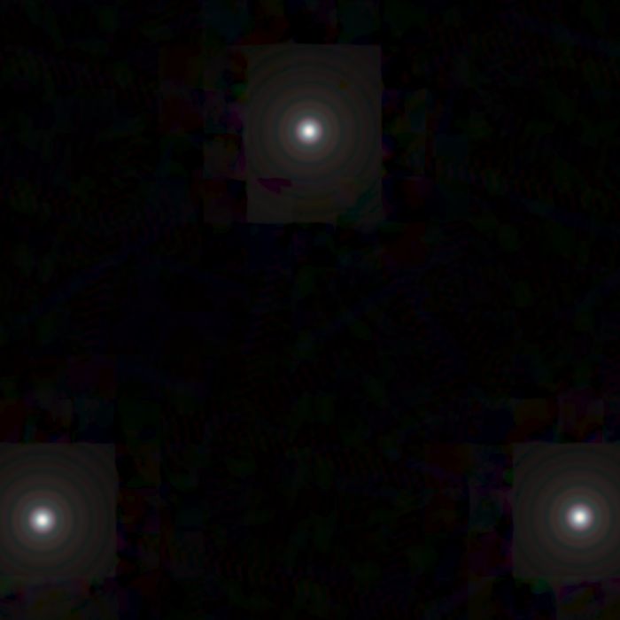
Figure 1: Coadded injected GalSim stars (left), white noise (center) and $1/f$ noise (right) realizations, displayed as 3-color F184 (red)/J129 (green)/Y106 (blue) combinations. Each image shows a $700\times 700$ output pixel ($17.5\times 17.5$ arcsec) region of the coadded images, from the gsstar14, whitenoise1, and 1fnoise2 layers, respectively. The color scale is a fourth-root stretch (0 to 0.2 input flux per input pixel) in the injected star image (left); and for the noise realizations it is linear, spanning $\pm 1.25$ (center) or $\pm 4$ (right) in input units. Note that the input white noise layer leads to output noise correlated on the scale of the input pixels, whereas the $1/f$ noise layer shows the characteristic striping at each of the 2 input rolls. These rolls are at different angles in each filter, hence the color pattern. The region shown is $270\leq x<970$, $301\leq y<1001$ of block (2,30).

Throughout this paper, we use the quantity called “fidelity” as the basic quality indicator of the Imcom output, and many statistics are reported as a function of the fidelity. This defines how well the output PSF recovered the target PSF we specified. Mathematically, fidelity depends on the difference between the output and target PSF,

$$L_{\alpha}({\mn@boldsymbol{s}})=\sum_{i=0}^{n-1}T_{\alpha i}G_{i}({\mn@boldsymbol{R}}_{\alpha}-{\mn@boldsymbol{r}}_{i}+{\mn@boldsymbol{s}})-\Gamma_{\alpha}({\mn@boldsymbol{s}}),$$ (1)

where the index $\alpha$ indicates an output pixel; $i$ indicates an input pixel; $G_{i}$ is the PSF in the $i$th input pixel; and ${\mn@boldsymbol{R}}_{\alpha}$ and ${\mn@boldsymbol{r}}_{i}$ are the output and input pixel positions. The fidelity is defined as the square norm of the output PSF residual scaled to the square norm of the target PSF, and re-written as an inverse logarithmic measure:

$${\rm Fidelity}\equiv-10\log_{10}\frac{U_{\alpha}}{C}\equiv-10\log_{10}\frac{\int[{L}_{\alpha}(\mathbf{s})]^{2}d^{2}\mathbf{s}}{\int[{\Gamma}(\mathbf{s})]^{2}d^{2}\mathbf{s}}.$$ (2)

The fidelity is usually — but not always — better (larger) if there are more exposures. The fidelity map in our simulation footprint for each bandpass we simulated can be found in Fig. 10 of Paper I.

3 Measurement of noise correlations

We first investigate the noise fields, giving an overview of noise effects (Sec. 3.1), and then describing the 2D (Sec. 3.2) and 1D azimuthally averaged (Sec. 3.3) noise power spectra.

3.1 Overview

Noise is a significant source of error for the precision necessary to observe weak gravitational lensing of galaxies. The impact of noise on the measurement of a shear signal can be parameterized into two types of systematic observational errors: additive and multiplicative biases (e.g. Heymans et al., 2006). If the true signal is given by $\gamma_{\rm true}$, noise (or other) biases give a $\gamma_{\rm meas}$ of

$$\gamma_{\rm meas}=(1+m)\gamma_{\rm true}+c.$$ (3)

The additive bias (also called “spurious shear”) is given by the constant c, and manifests as a shear signal that is present even when the true population of galaxies is unlensed. The factor of m gives the multiplicative bias (also called “calibration error”). Multiplicative bias occurs when a real lensing signal is detected, but the measurement is larger or smaller than the true signal by some factor (Bacon et al., 2001; Erben et al., 2001; Hirata & Seljak, 2003). The next-generation weak lensing surveys have stringent requirements for both types of errors (Paulin-Henriksson et al., 2008; Massey et al., 2013; Cropper et al., 2013; The LSST Dark Energy Science Collaboration et al., 2018; Euclid Collaboration et al., 2020; Troxel et al., 2021).

To quantify the impact that noise might have on observations and determine whether these requirements will be met, we measure and analyze noise correlations in the coadded images from two types of input noise fields: white noise and $1/f$ noise (see Sec. 3.4 of Paper I). Real noise has both of these components, as well as some smaller additional terms (Rauscher, 2015). We focus on the noise power spectrum in the output images, since both the lowest-order noise-induced bias and the variance of the measured shapes are proportional to second moments of the noise (i.e., depend on (S/N)^-2; Bernstein & Jarvis 2002) and are therefore captured by the power spectrum. We then compare this power spectrum to the expected output noise power spectrum if we ignored sampling issues. Appendix B describes in detail the impact of anisotropic noise (such as $1/f$ noise and non-ideal white noise) on ellipticity measurements.

Different properties of a galaxy are affected by noise at different wave numbers. If a large scale uniform (zero wavenumber) noise offset is present in an image, the error in this flux would impact the estimated photometric flux from the galaxy, but not the position or shape. An astrometric measurement will, however, be affected by an overall tilt (gradient of the noise, or in Fourier space the noise weighted by one factor of wavenumber); this would bias the centroid towards one direction or another. The shape of a galaxy will only be biased if the second derivative of the noise field is biased towards a preferred direction. In Fourier space, the ellipticity error thus comes from the noise weighted by two powers of the wave number (the impact of noise on shapes is discussed more in Sec. 4.5). Photometry, astrometry, and shape measurements are thus dependent on higher and higher spatial frequencies respective to one another. This is demonstrated quantitatively in Appendix B, including the factor of wave vector squared ($u^{2}-v^{2}$ for $g_{1}$ and $2uv$ for $g_{2}$) appearing in the noise-induced error in the shapes.

3.2 2D noise power spectra

We take the convention that the power spectrum $P(u,v)$ of a field is given by the 2D Fourier Transform of the correlation function $\xi(\Delta x,\Delta y)$:

$$P(u,v)=\int\xi(\Delta x,\Delta y){\rm e}^{-2\pi{\rm i}(u\Delta x+v\Delta y)}\,{\rm d}\Delta x\,{\rm d}\Delta y,$$ (4)

where $\xi(\Delta x,\Delta y)=\langle S(x,y)S(x^{\prime},y^{\prime})\rangle$ is the correlation function of the noise field $S$ with pixel coordinates given by $(x,y)$ in Cartesian space and $(u,v)$ in Fourier space. In the case of discrete data, we replace the integral with a sum over pixels; we preserve the convention that $P$ has units of $S^{2}\times\,$area (e.g., for a field sampled at the output pixel scale $s_{\rm out}$ as considered here, we sum over pixels and multiply by $s_{\rm out}^{2}$).

We accomplish this by making use of the Numpy Fast Fourier Transform (FFT) function (Harris et al., 2020). Each noise field in each $N\times N$ pixel block (here $N=2600$) is FFTed and normalized by the size of the blocks and the size of the output pixels:

$$P_{2D}(u,v)=\frac{s_{\rm out}^{2}}{N^{2}}\left|\sum_{j_{x},j_{y}}S_{j_{x},j_{y}}{\rm e}^{-2\pi{\rm i}s_{\rm out}(uj_{x}+vj_{y})}\right|^{2},$$ (5)

where $u$ and $v$ are sampled at integer multiples of $1/(Ns_{\rm out})$. The two-dimensional power spectra that result from this are further binned into $8\times 8$ bins, resulting in power spectra that are $325\times 325$ pixels covering the range of $u$ and $v$ from $-20$ to $+20$ cycles arcsec^-1 (the Nyquist limit for $s_{\rm out}=0.025$ arcsec/pixel) at spacing

$$\Delta u=\Delta v=\frac{1}{325s_{\rm out}}=0.123\,{\rm cycles\,arcsec}^{-1}.$$ (6)

For each observation filter, we then averaged together the power spectra from each of the 2304 blocks (the total $48\times 48$ arcmin² region). The resulting average power spectrum for the full mosaic in each observing filter can be seen in Fig. 2. Note that this procedure included the padding regions that appear in more than one block, so these regions are over-represented in the averaged power spectrum. Since the padding regions are not special relative to the detectors or tiling strategy, we do not think this is a major issue.

In the absence of sampling issues and if the input and output PSFs were all identical, input white noise should lead to output white noise and a constant power spectrum for the 2D image. Since we have an output PSF that is larger than the input PSF in real space (narrower in Fourier space), we expect that the high-wave number Fourier modes will have reduced power (proportional to the square of the Fourier transform of the output PSF). The examples in Figure 2 clearly show this behavior. Note that the spectra are plotted on a log scale, so that although several features are visible, any features outside of the central maxima have very little power. The circular region in the center of the 2D power spectra comes from the output PSF: the Airy disc convolved with a Gaussian. In the Y106 and J129 bands, where the Gaussian dominates the cutoff of the PSF, we see a smooth fade into uncorrelated wavenumber space. In the H158 band and especially the F184 band, the Airy disk defines the limit of the PSF, so beyond this limit the image contains only noise — this causes Imcom to set the background to zero, causing the hard edge of the circle.

We can confirm this by comparing measurements of the image with expectations. The band limit (maximum number of cycles per unit angle) for a diffraction-limited telescope is given by $D/\lambda$, where $D$ is the telescope diameter and $\lambda$ the wavelength of light. For the F184 band,

$$\frac{D}{\lambda}=\frac{2.37\,\text{m}}{1.84\,\mu\text{m}}=1.29\times 10^{6}{\rm\,cycles\,rad}^{-1}=6.25{\rm\,cycles\,arcsec}^{-1}.$$ (7)

This is indeed the radius of the circle on the F184 band image, confirming that this feature is caused by the Fourier modes outside the circular regions being beyond the target PSF band limits.

The large “$+$ signs” extended throughout the images correspond to the directions of the postage stamp boundaries. (Note that the input images are at various roll angles, so these features must instead be associated with the output.) The step function-like feature of the postage stamp boundaries becomes a continuous line in Fourier space, so we see these extended $+$ signs in the power spectra.

The spots in the F184 band are a small print-through of the initial pixel positions in the input images into the final output images. The first ring of 8 points is located at a radius of $\sim 9$ cycles arcsec^-1 from the center, i.e., roughly the inverse of the input pixel scale $s_{\rm in}=0.11\,$arcsec. As expected, the directions of the 8 points corresponds to the 4 grid directions of the input exposures.

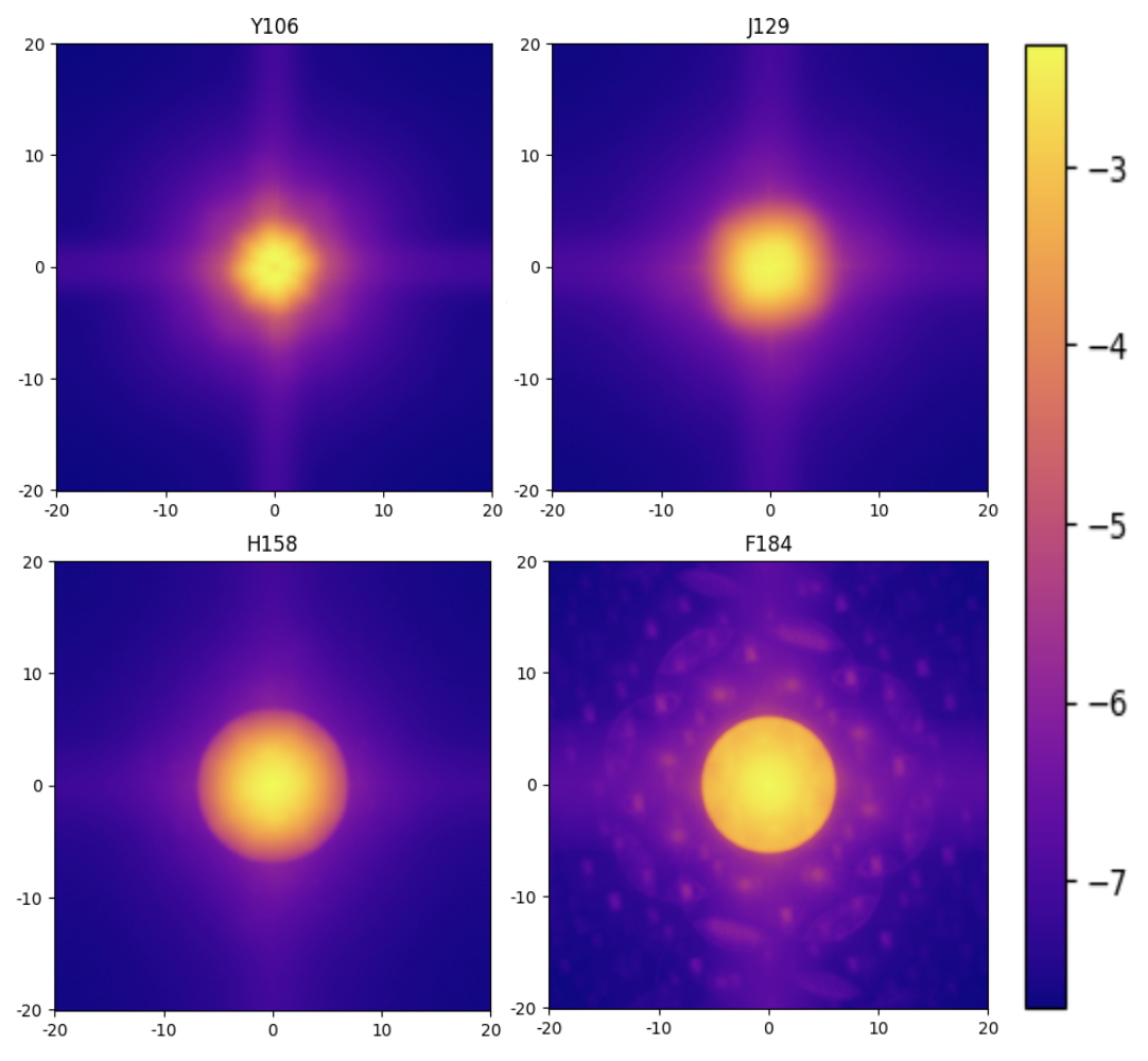
Figure 2: 2D averaged power spectrum of the white noise field of each band, plotted on a logarithmic color scale. The horizontal and vertical axes show wave vector components ($u$ and $v$ respectively) ranging from $-20$ to $+20$ cycles arcsec^-1. The color scale shows the power $P(u,v)$ in units of arcsec² (Eq. 4). The minimum and maximum values of each power spectrum are as follows: $6.6\times 10^{-8}$ to $6.7\times 10^{-3}$ for Y106; $3.4\times 10^{-8}$ to $3.5\times 10^{-3}$ for J129; $5.9\times 10^{-8}$ to $3.2\times 10^{-3}$ for H158; and $2.0\times 10^{-8}$ to $4.8\times 10^{-3}$ for F184.

For the $1/f$ noise power spectra in Figure 3, we have combined two sets of images with horizontal banding at different roll angles, so the output noise image will have at least two distinct preferred directions (see the right panel of Fig. 1). These features appear strongly in each panel of Figure 3 as a distinct X through the centers of the images. The roll angles are slightly different in each band in order to maximize coverage, leading to different orientations of the X’s in each image.

As in the white noise spectra, the boundary between postage stamps contained in the images creates step-like features in the noise fields, which manifest as two distinct perpendicular Fourier modes in the power spectra. However, this feature is clearly more prominent in the $1/f$ noise than in the white noise. In $1/f$ noise, we have striping across entire channels within the detector, which then crosses over postage stamp boundaries. The correlations between postage stamp boundary-caused features extend over much larger scales in real space, corresponding to sharper features in Fourier space. Thus we see the postage stamp boundary feature (the large $+$ sign) more distinctly in these images.

The $1/f$ bands also display the same reduction of power at large wave number as in the white noise, and the sharp circular boundary in H158 and especially F184 caused by the band limit of the PSFs.

In addition to features coinciding with behaviors seen in the white noise images, we see one additional pattern appear in the $1/f$ noise that is not present in white noise data. Figure 3 shows this feature most clearly in the J129 band: alternating bright and dark vertical fringes across the center of the 2D power spectrum image. We measure the spacing between fringes to be 0.8 cycles arcsec^-1, or one cycle per 1.25 arcsec postage stamp. We therefore believe that the fringes result from steps at the postage stamp edges, with a sense that is coherent across multiple postage stamps (due to the large correlation length of the $1/f$ noise).

While these rough analytical arguments allow us to identify specific features in the output 2D power spectra with properties of the input images and Imcom algorithm, the quantitative details — how much power appears in each feature, and how this varies as a function of sampling going from Y106 (bluest/worst sampled) to F184 (reddest/best sampled) — must be determined via simulations.

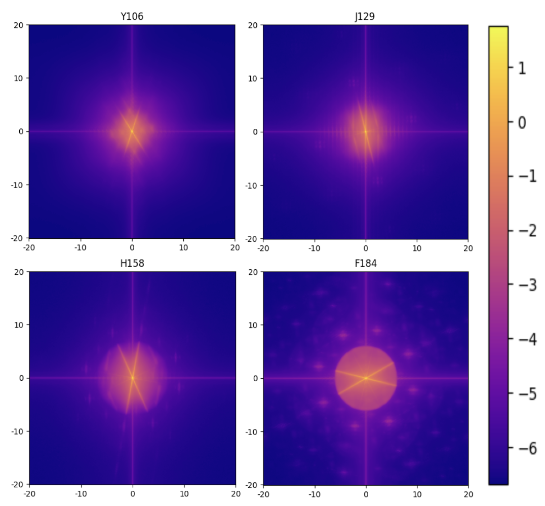
Figure 3: The 2D averaged power spectrum of the coadded $1/f$ noise field of each band, plotted on a logarithmic color scale. The horizontal and vertical axes show wave vector components ($u$ and $v$ respectively) ranging from $-20$ to $+20$ cycles arcsec^-1. The color scale shows the power $P(u,v)$ in units of arcsec² (Eq. 4). The minimum and maximum values of each power spectrum are as follows: $1.8\times 10^{-6}$ to $5.4\times 10^{1}$ for Y106; $8.5\times 10^{-7}$ to $4.6\times 10^{1}$ for J129; $6.9\times 10^{-7}$ to $4.8\times 10^{1}$ for H158; and $2.1\times 10^{-7}$ to $5.6\times 10^{1}$ for F184. The X-shape, $+$ sign, spots (in H158 and F184), and vertical fringes (in J129) are discussed in the main text.

3.3 Azimuthally averaged power spectra

In addition to the two-dimensional power spectra, we generate for each filter a set of one-dimensional azimuthally averaged power spectra. First, the two-dimensional power spectra of each block are saved from the previous step of analysis. We then calculate the mean exposure coverage in each block, and group the power spectra into one of 5 bins in mean coverage. Since the root-mean-square of noise in the output noise images shows the mean exposure coverage dependence, it is good to check how noise correlations depend on the coverage as well (see Sec. 5.3 of Paper I for more details). These power spectra are also separated by observing filter, as exposure coverage varies significantly depending on the band in which observations are taken. We average together the 2D power spectra for blocks within a given mean coverage bin into a single 2D power spectrum, which is then azimuthally averaged over thin annuli, using the method from Casey et al. (2023). For this work we used 162 radial bins, effectively taking rings of width one pixel in the power spectrum map (Eq. 6) and averaging the values of the power at each circular aperture of wavenumbers.

Figure 4 shows the mean coverage-binned 1D power spectra for the output white and $1/f$ noise images in each observation filter. Rather than just $P(\upsilon)$, we plot $2\pi\upsilon P(\upsilon)$ so that the area under the curve corresponds to the variance in the output pixels. We additionally include in each figure a purely analytical model of the 1D power spectrum, based on $N_{\rm in}=5$ input exposures and ignoring pixelization/sampling issues. Derivations of the analytical models for the output noise power spectra can be found in Appendix A.

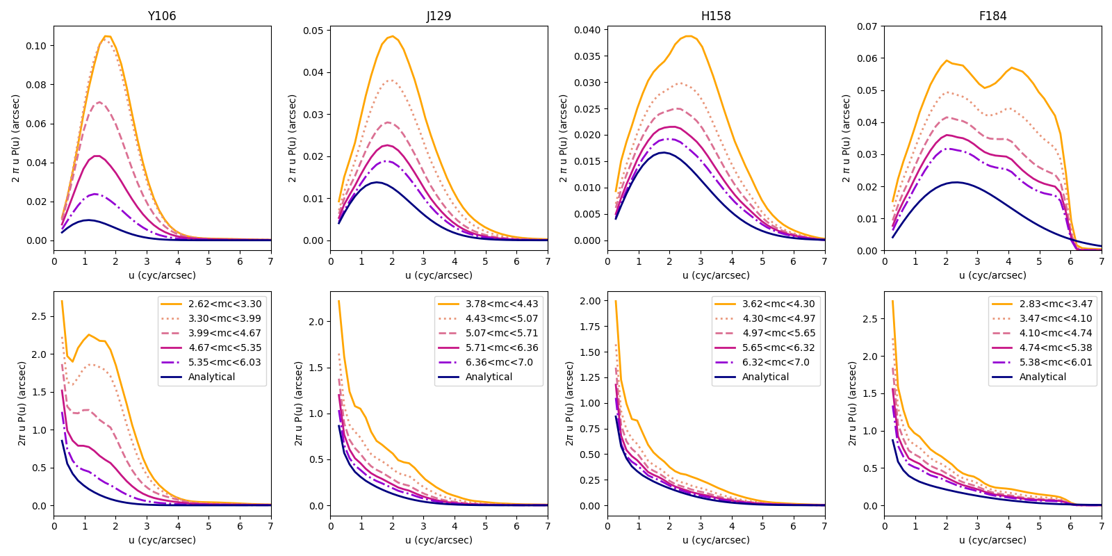
Figure 4: Top row: 1D power spectra for the output white noise fields in each filter. Bottom row: 1D power spectra for the output $1/f$ noise fields in each filter. Each filter’s spectra are divided into five even-width bins of mean coverage (“mc” in short), and plotted against the analytical expectation for noise power spectra for combining 5 exposures in the absence of sampling issues (see Appendix A for derivations).

For all bands and for both types of noise, the peak power and width of the power spectrum depends consistently on the mean coverage in the image. Exposures with small mean coverage values have the highest peaks and the slowest dropoffs down to zero power at large wave number. Our analytic expectation represents an idealized case, and the behavior as compared with the spectra for the mean coverage bins shows that with decreasing mean coverage, we move farther above the ideal power spectrum. However, we note that in all of these cases the noise power spectrum is above the analytic expectation for most wave numbers.

In the white noise 1D power spectra, several features are evident in all bands. Each of the observation bands shows that the contributions to the power spectrum (weighted by $2\pi\upsilon$) go up, rise to some peak, and come back down to zero, qualitatively consistent with the analytic expectation. Noise increase due to aliasing often gets worse as one moves to larger wave number (the zero-mode corresponds to total flux, which is conserved in the absence of intrapixel sensitivity variation). This can result in $2\pi\upsilon P(\upsilon)$ having a steeper dependence than $\propto\upsilon$ at small $\upsilon$, as seen prominently for Y106 (the most undersampled filter) in Fig. 4. Figure 5 shows the central feature in the 2D power spectrum from input white noise for each filter with the color scale significantly stretched to show this behavior.

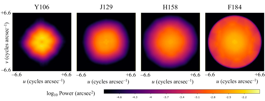
Figure 5: Zoomed in image of the central features in the input white noise power spectra. By stretching the color scale we can see more clearly that the zero-wavenumber modes do not contribute the most to power in the output noise, particularly in Y106.

In contrast, the $1/f$ noise spectra have a distinct peak in the center of the image, caused by the overlaps in the Fourier modes from the roll angles. The power spectrum as a function of frequency on one dimension goes like $1/f$, so for small wave numbers the power should reach very large values — a result that is clearly visible in the spectra for all bands. The analytic estimation for the $1/f$ noise spectra in the absence of pixelization/sampling effects (Appendix A) is qualitatively correct for the redder filters, but the normalization is slightly low, and it misses the “bump” caused by aliasing in the bluer filters (especially Y106).

Analyzing these power spectra allows us to understand the correlations between features caused by noise in the simulated images being operated on by Imcom. In Section 4.5, we provide a more detailed discussion of the quantitative links between these power spectra and weak lensing measurement biases.

4 Moments Analysis of the coadded images

In this section, we present the quantitative analysis of the simulated coadded images of multiple layers. This includes object centroid, ellipticity and size measured by computing image moments of objects located in grids, and simulated fields with and without noise.

4.1 Moments of the injected sources

Our first set of tests is conducted on the grids of simulated stars. Our main objective is to show the properties of the output PSFs and demonstrate that these properties have an expected dependency on how divergent the output PSF is from the target. The expected properties are exactly known since we chose the target PSF to be the Airy disk convolved with the Gaussian kernel.

Our simulation footprint contains 54 597 unique simulated stars, each at the center of a HEALPix (Górski et al., 2005) resolution 14 pixel. For each injected star, we cut out a $99\times 99$ output pixel (2.475$\times 2.475$ arcsec) postage stamp from the output block containing that star (for the “block” definition refer to Fig. 4 of Paper I). We consider the first the GalSim noiseless star layer (gstar14). We measure the $1^{\rm st}$ and $2^{\rm nd}$-order moments of the simulated sources in the output images using the galsim.hsm module (Hirata & Seljak, 2003; Mandelbaum et al., 2005), which implements the fitting of an adaptive elliptical Gaussian to the image (e.g. Bernstein & Jarvis, 2002). The $1^{\rm st}$ moments (centroids) can be compared with the expected position based on the World Coordinate System (WCS) of the coadded image; the result is reported as the astrometric error. The $2^{\rm nd}$ moments (covariance of the Gaussian: a $2\times 2$ matrix M) are reported as three real numbers: the shear-invariant width

$$\sigma=\sqrt[4]{M_{xx}M_{yy}-M_{xy}^{2}},$$ (8)

and the shape components

$$(g_{1},g_{2})=\frac{(M_{xx}-M_{yy},2M_{xy})}{M_{xx}+M_{yy}+2\sqrt{M_{xx}M_{yy}-M_{xy}^{2}}}$$ (9)

that are zero for a perfectly circular object and generally satisfy $g_{1}^{2}+g_{2}^{2}<1$ for a positive definite second moment matrix. (The use of “$g$” for the latter indicates consistency with the conventions of Schneider & Seitz 1995.) We also report the mean fidelity $\langle-\log_{10}(U_{\alpha}/C)\rangle$ for the pixels in the central $20\times 20$ output pixel (i.e., $0.5\times 0.5$ arcsec) region surrounding the star. This is a measure of how well Imcom estimates it has done at building an output image with the desired PSF in that region of the survey.

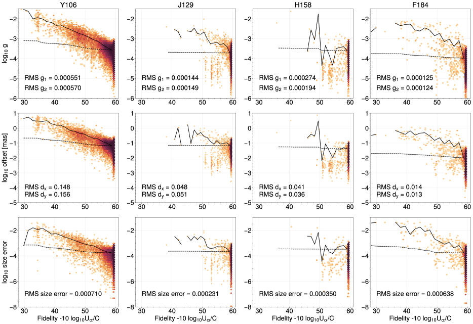
Figure 6: The distributions (in an arcsinh scale) of moments of the injected stars drawn in the input images, coadded in Imcom, and then measured by the galsim.hsm module in each of the filters, with no noise. Top: the ellipticity $g=\sqrt{g_{1}^{2}+g_{2}^{2}}$ of the injected GalSim stars. Middle: the astrometric displacement from the coordinates where the star was injected. Bottom: the relative size error of the GalSim stars and target PSF. The definition of size in this figure is Eqn. 8. The horizontal axis is the output PSF fidelity (larger means a better match to the target PSF; see Sec. 2). The solid line shows the RMS ellipticity (top), RMS astrometric displacement (middle), and RMS fractional size error (bottom) in each fidelity bin. The dashed line is the same thing but is cumulative (i.e., the RMS for all stars in regions with that fidelity or better). This would be applicable to cases where we impose a mask based on the fidelity.

Figure 6 shows measured ellipticity, astrometric error and fractional size difference of the sources drawn by GalSim. It is expected that the anisotropy of shapes decreases as the fidelity of the output image is maximized. Most of the postage stamps (for the “stamp” definition refer to Fig. 4 of Paper I) achieved high fidelity (above 50) in all bandpasses except Y106. This is likely due to the bandpasses being the most undersampled and that the algorithm is unable to find the transformation matrix that the leakage and noise correlations are minimal (this is also shown in Fig. 11 of Paper I). In all bandpasses, however, the total RMS ellipticity of the coadded injected stars in each shape component is $\lesssim$ $5.7\times 10^{-4}$ which is the PSF ellipticity requirement on angular multipole scales (32 < $\ell$ < 3200) determined by the SRD. Here we also demonstrate that the astrometric error of the sources induced by Imcom is a small contribution to the relative error budget in the astrometric calibration ($<1.3$ mas) defined by the SRD. Finally, the bottom panel of Fig. 6 shows the fractional size error of the injected stars relative to the target PSF. We cannot directly compare the RMS size error in each bandpass to the required PSF size error in the SRD ($\lesssim$ $3.6\times 10^{-4}$) because our RMS errors are computed at individual points, whereas the size error requirement is computed at scales $\ell<3200$ (or smoothed at a scale of $\sim 4$ arcmin, i.e., where there are $3200^{2}$ pixels on the full celestial sphere). We see that the size errors are largest in Y106 and F184. If we bin the stars into pixels, we see that the size error declines to $(1.58,0.59,1.01,2.09)\times 10^{-4}$ in Y106/J129/H158/F184 respectively in $1\times 1$ arcmin pixels; and then it declines to $(0.46,0.39,0.70,1.46)\times 10^{-4}$ in $4\times 4$ arcmin pixels. Thus we see that the image combination step is using only a small fraction $(1.46/3.6)^{2}=16\%$ of the overall PSF size error budget in a root-sum-square sense.

The spatial distribution of the second moment errors, averaged in 1 arcmin² pixels, is shown in Fig. 7. Most of the area has ellipticity errors at the $\lesssim 10^{-4}$ level; one sees a few outliers, with corresponding errors in the size. The large outliers seen in Y106 and F184 correspond to low-coverage regions (see Fig. 1 of Paper I). What matters most for weak lensing purposes are the 2-point statistical features of these maps; the correlation function will be investigated in Sec. 4.3.

Figure 7: A spatial map of the size error (color scale) shape (whiskers) of the injected stars. Each panel shows the $48\times 48$ arcmin footprint of the simulation in one of the 4 filters. Stars are averaged into pixels (1 arcmin² each). The color scale shows size error $(\sigma_{\rm star}/\sigma_{\rm target}-1)$ on an arcsinh scale, and the whiskers are scaled so that a length of 1 pixel corresponds to $g=5\times 10^{-4}$. This is presented on a square grid, however we have checked that the main features are also present if gridded in HEALPix and so they are not gridding artifacts.

We note that these quantities are also measured on the sources drawn by our internal “croutines” and we find consistent results as GalSim sources.

4.2 Measurement of stars in the simulated images

For precise measurements of galaxy properties, of particular interest is the propagation of the PSF through coaddition algorithms. In principle, Imcom tries to remove any anisotropy or inhomogeneity from the coadded PSF and coadd stars should result in being round. However, since the leakage (square norm of the difference of output and target PSF) is not exactly zero there is some residual ellipticity of the coadded stars even in the absence of noise. Although stars in the coadded images are not utilized directly for modeling the PSF (with Imcom, the PSF determination step must be performed on single-epoch images prior to coaddition), the coadded stars are an important test of PSF propagation and any ellipticity that we see at the end will have implications for galaxy measurement.

Stars are identified in the coadded sky images based on the truth locations of these stars. We use the simple simulated sky images for Roman simulated in Troxel et al. (2023), which utilized the LSST DESC DC2 simulations (LSST Dark Energy Science Collaboration (LSST DESC) et al., 2021b). Its stellar catalog was based on Galfast (Jurić et al., 2008; Jurić, 2018) simulations. We cut out postage stamps around the truth locations and measure the star properties using the galsim.hsm module (which allows the flux, centroid, and second moments to float). The truth catalog contains locations, magnitudes estimated in Roman bandpasses from object flux based on objects’ SEDs, and whether the star is a candidate for PSF modeling. The criteria for being a candidate star defined in Troxel et al. (2023) are that:

• no pixel in the simulated star stamp is saturated in at least one exposure of the star (saturation was chosen at $10^{5}$ e in the images with simple detector models); and

• the star has a detection signal-to-noise (S/N)_det above 50, as defined by (S/N)_det = $0.015\times(\rm total\ flux)$, where 0.015 was the typical background inverse noise level. (The observed signal-to-noise ratio including source Poisson noise is slightly lower.)

The S/N level was chosen here to be permissive to allow more restrictive selections later. We used this criteria for selecting clean stellar samples to conduct our measurement. We additionally select stars whose magnitudes are fainter than 18 in all bandpasses since we found that some single-exposure images contained saturated stars. (In the real survey, some information might be obtained from saturated stars because the detectors are read non-destructively and the early, non-saturated reads can be used; however, it is possible that the PSF would be different since one does not average over telescope motion during the full exposure, and in any case the present simulations do not include the early reads.)

With these selections, we consider 2623 (Y106), 2674 (J129), 2588 (H158), 2647 (F184) stars in our simulation footprint. For each star in each of the Imcom images (SCI and truth), we cut out $99\times 99$ output pixels postage stamps resulting in a stamp 2.475 arcsec on each side, whereas we extract $43\times 43$ pixels around the truth centroid of a star in Drizzle images resulting in a stamp 2.473 arcsec on each side. Although the cutouts from Drizzle coadded “SCI” images (Drizzle: SCI) are directly comparable with those of Imcom coadded “SCI” images (Imcom: SCI), the measurements of stars on “truth” images are not. While we cut out postage stamps from Imcom coadded “truth” images (Imcom: truth), Drizzle coadded images of the “truth” layer were not simulated by Troxel et al. (2023) at the time of this project. Examples of Imcom and Drizzle images are shown in Fig. 8.

Figure 8: Coadded images of SCI and truth layers for a selected region for Y106, J129, H158 and F184 bandpasses. Left: Drizzle co-added SCI image, Middle: Imcom co-added SCI image. Right: Imcom co-added truth image. The flux in Drizzle images are scaled by (0.11/0.0575)² to account for the difference in the output pixel size and normalized to show the same color range. The area that is shown here is $32.7\times 19.2$ arcsec centered around RA$=53.006\,$deg and Dec$=-40.027$. Note that this is near the center of our simulated output region.

Compared to the measurement of injected stars (Sec. 4.1), the measurement on the cutout of stars is expected to contain complications that could directly affect the shape and size of an object. These complications include background and simulated-detector noise, blending, and chromaticity (since the injected sources are drawn with the same SED passed to Imcom, but the simulated stars are drawn with their “true” SEDs). The simulated stars therefore test more of the sources of systematic biases in weak lensing surveys. Some of these effects can be seen in Figure 9 as outliers from the stellar locus in each bandpass. Fig. 9 additionally displays stellar locus of the same stars in Drizzle images, which is located at a smaller size than Imcom stars. This is expected because Drizzle does not smear the PSF. However, there is a large dispersion in sizes especially in the bluer, more undersampled bands. The Drizzle algorithm is designed to preserve total flux in its “raining down” procedure (Fruchter & Hook, 2002), but the spatial spread in the output image will depend on the specific locations of the pixels. Even though the output PSF from Imcom is larger than Drizzle (especially in Y106), it is designed to be uniform: it must be large enough so that that output resolution could be achieved even in a part of the image where the pixels interlace each other differently (see Paper I, Fig. 7). The Imcom output PSF is still much smaller than ground-based PSF and the narrowness of the locus will help with star-galaxy separation in the real mission.

Figure 9: Size-magnitude diagram for the selected stars (mag$>18$) in our simulated Imcom and Drizzle images. The size of the stars is measured with the adaptive moments method (Bernstein & Jarvis, 2002). Note that Imcom produces a larger output PSF, but it is much more uniform (see main text).

Figure 10 shows the measured ellipticity of stars found in simulated images as a function of object magnitude. The mean ellipticity components $g_{1}$ and $g_{2}$ in Imcom are at the level of a $\lesssim$few$\times 10^{-4}$ for all bandpasses. By comparison, the measured shapes on Drizzle images are consistently different from zero by an amount of order $\sim 10^{-2}$ (Drizzle: SCI). It shows that the Drizzle process is not able to average out the shape of PSFs, regardless of the fact that output pixel size is larger in Drizzle images (0.0575 arcsec/pixel) than Imcom (0.025 arcsec/pixel) and pixel size does have an effect on the measured PSF ellipticity (Fig. E1 of Troxel et al. 2021).

Figure 10: The mean ellipticity ($g_{1}$, $g_{2}$) of PSF candidate stars as a function of star magnitude of corresponding bandpass is shown. Four colored data points in a panel show the values from the stars found in Y106, J129, H158, F184 images. These stars were cut out from mosaics of coadded images using the coordinates from truth star catalog. The magnitude is also taken from the truth catalog. The ellipicity is measured with adaptive moments method in GalSim and the error bar is a standard error of the mean. Top: the ellipticiity ($g_{1}$) from the cutouts of three sets of images (Imcom and Drizzle coadded SCI images, Imcom coadded truth images. Bottom: $g_{2}$ for the same set of stars. We use the Drizzle images produced in Troxel et al. 2023.

Figure 11: The residual ellipticity ($g_{1}$: Top, $g_{2}$: Bottom) of the stars extracted from several layers of simulated images is presented. Left: the difference in the shapes from Imcom coadded SCI and truth images. This shows the effect of simple noise models on the ellipticity as SCI images include them and truth images do not. Right: the difference in the shapes from the Imcom coadded SCI images and target PSF we chose in our Imcom simulations. This shows the cumulative effect of noise in sky images and output PSF fidelity.

Figure 11 shows the residual ellipticity measured on the cutouts of stars from “SCI” and “truth” images, and the ellipticity compared to the target PSF for Imcom (which in this case is only different from zero due to numerical precision). The difference between “SCI” and “truth” shows the residual shape introduced by the simple detector physics noise model (which includes dark current, saturation, and read and Poisson noise). Here, the average residual ellipticity is $\lesssim$ $2\times 10^{-4}$ for bright stars and $\lesssim$ $8\times 10^{-4}$ for faint stars, verifying that Imcom shows a tolerance to simple noise models on star shapes. We also investigated whether achieving the target fidelity can affect star shapes of different magnitudes. The right column of Fig. 11 that shows the cumulative effect of noise and fidelity indicates that for $g_{1}$ the residual behavior is consistent with the simple noise model case (top left panel of the same figure) whereas $\Delta g_{2}$ shows a non-zero residual ellipticity over a range of magnitude. Although this is likely caused by the output PSF that did not exactly match the target, the leakage into star shapes is less than the PSF ellipticity error requirement.

Additionally, we have estimated the magnitudes of the stars from the total image intensity for best-fit elliptical Gaussian in GalSim. These magnitudes are estimated on the stars of both Imcom and Drizzle “SCI” images. Figure 12 shows the relative error of the measured magnitude compared to the truth for each filter. It is estimated from the photon flux in the following way. The measured number of photons ($N_{\rm star}$) can be used to measure the magnitudes of the stars, using

$$m_{AB}=-2.5\log_{10}\frac{N_{\rm star}}{N_{\rm zero~{}point}}-m_{\rm correct},$$ (10)

where $N_{\rm zero~{}point}$ is the number of photons that Roman would observe for a 0 AB magnitude source (Oke & Gunn, 1983) and $m_{\rm correct}$ is an aperture correction term to account for the fluxes in the wings of stars, because the diffraction wings of the PSF are not captured by the best-fit Gaussian; thus the HSM fluxes are less than the “total” (integrated to $\infty$) fluxes. We compute the zero point based on the model throughput curve of Roman that was used in the simulation:

$$N_{\rm zero~{}point}=\int(3.631\times 10^{-23}\,{\rm W\,m^{-2}\,Hz^{-1}})A_{\rm eff}(\lambda)t_{\rm obs}\frac{{\rm d}\nu}{h\nu},$$ (11)

where $A_{\rm eff}$ is the effective collecting area of the telescope for a given bandpass, $t_{\rm obs}=139.8\,$s is the exposure time, and $h\nu$ is the energy of photons (where $h$ is Planck’s constant). The effective collecting area for a given bandpass can be integrated over the bandpass, and $\int(A_{\rm eff}/\lambda){\rm d}\lambda$ = 0.5915, 0.6051, 0.5978, 0.3929 m² for Y106, J129, H158, and F184 respectively. We then correct for $m_{\rm correct}$ by measuring the flux and magnitude on the target PSF for each bandpass; the corrections are 0.0977, 0.1471, 0.2180, 0.3018 mag for Y106, J129, H158, and F184 respectively.

Since we specify the target PSF in Imcom to be the Airy disk convolved with the Gaussian kernel, the adaptive moments method captures the fluxes from these stars quite well. Their RMS residual magnitudes are 28, 32, 41, 51 mmag in Y/J/H/F band whereas the SRD states relative photometric calibration in each filter to be better than 10 mmag. We should note that this measurement includes neighboring fluxes from nearby sources (which are not included in the SRD requirement) and stars with low fidelity (outliers in Fig. 9). A visual inspection of outliers from the size-magnitude diagram in Y106 showed that most are due to leaking flux from neighboring objects (not necessarily fully blended). For the adaptive moment magnitudes measured on Drizzle images, on the other hand, as the dispersion in the difference suggests, the coadded PSF obtained through Drizzle is not uniform across our footprint and the magnitude measurement is not reliable in the strongly undersampled case (Y106). (We note that Drizzle preserves total flux by construction; but the fraction of the flux captured by the adaptive moment method depends on the PSF.) Even for the weakly undersampled cases, the mean of the residual magnitude is one order of magnitude worse than the Imcom case.

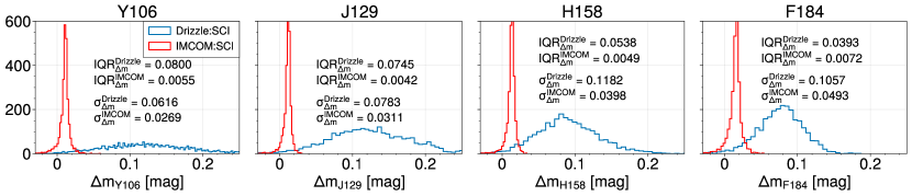
Figure 12: The deviation of measured magnitudes of the stars in Drizzle and Imcom images from the magnitudes from the truth catalog for all the bandpasses is shown. The magnitude of the stars is estimated from the flux measurement using galsim.hsm. Since the flux units in GalSim are photons/cm²/s, we multiply the flux measured on Imcom star cutouts by (0.025/0.11)² to obtain flux from surface brightness. There is no need for this scaling for Drizzle cutouts because Drizzle operates on fluxes rather than surface brightnesses. The number of photons is then converted to the AB magnitude through Eq. (10). The texts in each panel display the interquartile range (IQR) to indicate the spread that is unaffected by outliers, and the standard deviation of the sample.

In this section, we have only explored the moments on single-band images; the moments measured on multi-band (synthetic wide-band) images will be analyzed in Sec. 5.

4.3 Correlation functions of stars in various outputs

We have so far looked at one-point statistics of observed properties of stars in the coadded images of various input layers. In the end, however, it is crucial to verify that systematic biases related to undersampling and the image reconstruction process do not contaminate the cosmological signal (e.g., Fig. 12 of Troxel et al. (2023) for their estimated $\xi_{\pm}$ over 20 deg² simulated sky). We approach this by measuring two-point statistics, especially shape-shape correlations of these stars. The calculations of two-point correlation functions were performed using the publicly available TreeCorr package (Jarvis et al., 2004).

In Fig. 13, we measure shape-shape correlations ($\xi_{+}$) of observed stars in Imcom coadded injected stars and “SCI” layers, and in Drizzle coadded “SCI” image. We also show a simple comparison of these star shape correlations to Roman PSF mitigation requirements. Here we compute the approximate requirement on $\xi_{+}$ from the requirements on additive errors in SRD in each angular multipole moment bin. We rewrite the Hankel transform of angular power spectra $C_{\ell}$ as a Riemann sum (Givans et al., 2022):

$$\xi_{\rm+}\!\!\!\! = \!\!\!\!\int_{0}^{\infty}\frac{\ell\,{\rm d}\ell}{2\pi}\,J_{0}(\ell\theta)(C_{EE}(\ell)+C_{BB}(\ell))$$ (12)

$$\approx \!\!\!\!\sum_{\ell~{}\rm bins}2\gamma^{2}\langle J_{0}(\ell\theta)\rangle,$$

where $J_{0}$ is the Bessel function of first kind. It is clear here that the shape correlations of Imcom coadded stars are at a statistically acceptable level compared to the requirement. The most idealized case is shown as the correlations of injected stars, drawn with exactly the same input PSF given to Imcom: here any deviations of the measured shapes from isotropy and homogeneity can be attributed to the algorithm itself. We confirm that the level of correlations is two orders of magnitude smaller than the estimated systematic requirement. As can be seen in Fig. 13, disparities exist between $\xi_{+}$ on Imcom: SCI and Imcom: injected stars since the stars drawn in the noiseless injected source layer are isolated and the PSFs are made with a flat SED, while the stars drawn in Troxel et al. (2023) are fully chromatic. We should note that we do not expect the measurement using Drizzle stars to be consistent with zero since Drizzle does not attempt to smooth the output PSF to be isotropic.

It is worth mentioning that the $\xi_{\rm+}$ presented here is the contamination solely from star or PSF shapes — error contributions from residual PSF shape/size errors and shape measurement are not included. We consider the shapes of the injected stars as $e_{\rm PSF}$ and those of stars in sky image as $e_{\rm star}$. Typically we characterize the additive shear systematics as the following in terms of observed shear, PSF modeling errors and noise:

$$\gamma^{\rm obs}=\gamma^{\rm true}+\delta e^{\rm sys}_{\rm PSF}+\delta e_{\rm noise};$$ (13)

here $\delta e^{\rm sys}_{\rm PSF}$ (additive shear systematic biases due to PSF modeling) can be decomposed into

$$\delta e^{\rm sys}_{\rm PSF}=\alpha e_{\rm PSF}+\beta(e_{\rm star}-e_{\rm PSF})+\eta(e_{\rm star}\frac{T_{\rm star}-T_{\rm PSF}}{T_{\rm star}})$$ (14)

following Paulin-Henriksson et al. (2009) and Jarvis et al. (2016). Our test in this section only quantifies the contribution to $e_{\rm PSF}$ from residuals in the image combination process, but not the coefficients $\alpha$, $\beta$, and $\eta$. This will be investigated in a future paper. We will, however, quantify the contribution to the observed shear due to additive noise biases ($\delta e_{\rm noise}$) in Sec. 4.5.

Fig. 13 additionally demonstrates the tangential shear around the positions of simulated (in the “SCI” image) stars and the injected stars. While we expect these signals to be zero given that we have not put large scale structure in the position catalog and they seem to be below the additive shear error requirement (only in $2.0<\log_{10}\ell<2.5$ due to the relevant scale of galaxy-galaxy lensing), $\gamma_{\rm t}$ signal around injected stars might be underestimated because the angular distance between sources is discrete.

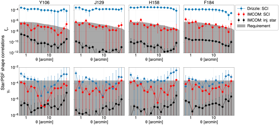
Figure 13: Top: Auto-correlation ($\xi_{+}$) of observed star ellipticity from various coadded images. This includes Drizzle and Imcom images with simple detector noise models (see Sec. 2 for detailed explanation), and GalSim-drawn injected stars from Imcom images. The ellipticity was measured with adaptive moments. Dark grey shaded region shows the required $\xi_{+}$ signal approximated with the requirements on additive shear errors from SRD. Each panel displays the signals corresponding to each bandpass, and “diamond” marker is the positive signal while “square” is the negative signal but taken absolute value. Bottom: Cross-correlation of the sky coordinates and the observed ellipticity of the same sources. Readers may refer to Fig. 7 for the residual ellipticity around the positions where there are fewer dither positions.

4.4 Correlations of fourth moments

In addition to the PSF second moments, Zhang et al. (2023c) demonstrated that the correlation function of the spin-2 components of the PSF higher moments (e.g., fourth moment) can cause shear additive bias to cosmic shear correlation function, contingent on the shear estimation method used in the analysis. We measure the standardized higher moments defined in Zhang et al. (2023b),

$$M_{pq}=\frac{\int\mathrm{d}x\,\mathrm{d}y\,u^{p}\,v^{q}\,\omega(x,y)\,I(x,y)}{\int\mathrm{d}x\,\mathrm{d}y\,\omega(x,y)\,I(x,y)}.$$ (15)

Here the $(u,v)$ are transformed coordinates from the image coordinate $(x,y)$, such that the second moment shapes in Eq. (9) vanish, and the second moment size in Eq. (8) is normalized to 1; $p$ and $q$ are the integer moment indices. For fourth moments, $p+q=4$. Here $\omega(x,y)={\rm e}^{-{\mn@boldsymbol{x}}\cdot{\textbf{{M}}}^{-1}{\mn@boldsymbol{x}}/2}$ is the adaptive weight function given by HSM (Hirata & Seljak, 2003), and $I(x,y)$ is the image of the PSF. The complex spin-2 fourth moment is defined as

$$M^{\rm(4)}_{\rm PSF}=M_{40}-M_{04}+2{\rm i}(M_{31}+M_{13}).$$ (16)

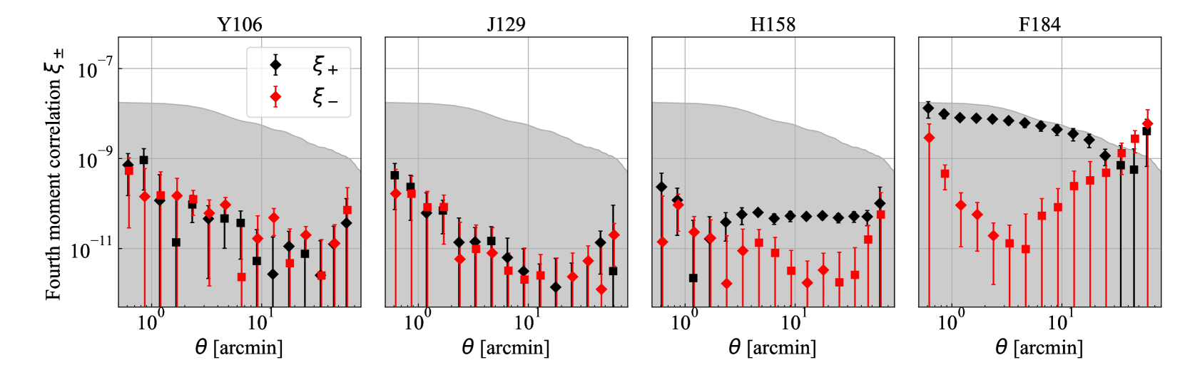
Figure 14: Auto-correlation ($\xi_{\pm}$) of the fourth moment spin-2 components ($M^{\rm(4)}_{\rm PSF}$), measured by the injected stars drawn from the GalSim routine. Each panel displays the signals corresponding to each bandpass, and “diamond” marker is the positive signal while “square” is the negative signal but taken absolute value. The grey-shaded region shows the requirement on the fourth moment $\xi_{+}$, computed from the SRD and the assumption that the fourth moment leakage will be $6$-times larger than that of second moments. The PSF fourth moments correlation functions are safely within the requirement for Y106, J129, and H158 band, and are on par with the requirement for the F184 band.

In Figure 14, we show the correlation function $\xi_{\pm}$ of the PSF fourth moments, measured on the coadded image of the injected stars drawn from the GalSim routine. This is presented with an approximated requirement for the fourth moments correlation function from the SRD, by assuming the fourth moment leakage factor $\alpha^{\rm(2)}$ is 6 times larger than the second moment leakage factor ($\alpha$ in Eq. 14). This decision is supported by the results of Zhang et al. (2023c). The fourth moment correlation function of the injected stars are safely within the requirement for the Y106, J129, and H158 band, showing that the higher moments of the anisotropy of the Imcom PSF will not cause significant additive bias in these bands. However, the correlation functions in F184 are only slightly below the requirement for the most angular range and are above the requirement (though not by a statistically significant amount) for the largest scales. This indicates that the PSF fourth moments could potentially contaminate the real cosmological signal in F184. In fact, the fourth moments correlation function is $\sim 3$ order-of-magnitude larger than the second moment correlation in terms of signal-to-requirement fraction, mainly because Imcom PSFs have extremely low large-scale coherence in the second moment shapes, which is not necessarily the same for the fourth moments.

This result suggests that the PSF fourth moments should be actively monitored in the Roman HLIS cosmological analysis. Further work is however required for investigating the leakage of PSF fourth moments into the galaxy shape for the Roman HLIS, by cross-correlating the galaxy shape with the star moments (characterization of the $\alpha,\beta,\eta$ coefficients in Eq. 14). A larger-area simulation will also be valuable here for better understanding the leakage at scales larger than 60 arcmin.

4.5 Estimation of additive noise bias

A concern with measuring shapes on a coadded image is that noise correlations can result in a bias in the shape measurement even if the PSF has been made round and is exactly known (Kaiser, 2000; Bernstein & Jarvis, 2002; Hirata et al., 2004; Refregier et al., 2012; Melchior & Viola, 2012; Mandelbaum et al., 2015; Gurvich & Mandelbaum, 2016; Herbonnet et al., 2017; Okura & Futamase, 2018). For example, if there are noise correlations in the $x$-direction, then there are different centroid uncertainties in the $x$ and $y$ directions; this propagates into different biases in object moments $\langle x^{2}\rangle$ and $\langle y^{2}\rangle$, and hence a bias in the ellipticity $g_{1}$. There are in fact a number of such terms, each resulting from the fact that the ellipticity is a non-linear function of the data, and leading overall to a bias proportional to $\nu^{-2}$ where $\nu$ is the detection significance (see, e.g., the detailed discussion in Bernstein & Jarvis 2002, §8.2). This results in the additive noise bias; the aforementioned leading terms result from the second derivative of the measured shape with respect to the input image, and so we refer to it as the “second-order” additive noise bias. (There are third-order and higher terms as well.) A more detailed treatment will be presented in a future paper; here our aim is a first look at the second-order noise bias of the ellipticities of injected stars.

One may construct a Monte Carlo estimate of the additive bias as follows:

$$\Delta g\!\!\!\! = \!\!\!\!\frac{1}{2}\sum_{\alpha\beta}\frac{\partial^{2}g}{\partial I_{\alpha}\,\partial I_{\beta}}{\rm Cov}(I_{\alpha},I_{\beta})$$ (17)

$$\approx \!\!\!\!\left\langle A\left[\frac{g(I+\epsilon N)+g(I-\epsilon N)}{2}-g(I)\right]\right\rangle,$$

where $I$ is the image of the object; $N$ is a noise image; $A$ and $\epsilon$ are scaling factors; and the $\langle\rangle$ denotes an average over the Monte Carlo noise realizations. If the shape measurement of the object is performed on a coadded image, then $I$ should be the coadded image and $N$ should be a coadded noise realization (and thus includes any correlations imprinted by the coaddition procedure).

If the object image is normalized to have unit flux, and $N$ is normalized to be a noise image with unit input variance per input pixel, then the proper scaling is

$$A\epsilon^{2}|_{\rm white~{}noise}=\frac{1}{\nu_{\rm SE}^{2}\Omega_{\rm psf}/s_{\rm in}^{2}},$$ (18)

where $\nu_{\rm SE}$ is the single-epoch signal-to-noise ratio and $\Omega_{\rm psf}/s_{\rm in}^{2}$ is the input PSF effective area in pixels (shown in Table 4 of Paper I). Then Eq. (17) returns an estimate of the second-order additive noise bias. In principle, the use of multiple Monte Carlo realizations of the noise should allow us to reduce the uncertainty in Eq. (17). But even a single realization is unbiased and can be used in a correlation function code such as TreeCorr to estimate the additive noise bias correlation function.

There may also be noise bias from the input $1/f$ noise. Typically the $1/f$ noise is specified by a “knee frequency” $f_{\rm knee}$ (with the pixels time-ordered, so units of Hz) where the $1/f$ noise power spectrum is equal to the white noise component power spectrum. For readout, the $4096\times 4096$ pixel arrays used by Roman split into 32 channels of 4096 rows and 128 columns each. The pixels in each row are read out with a cadence of 5 $\mu$s; after all the pixels in one row are read out, we move to the next row (so the time to read each row is $128\times 5=640\,\mu$s plus overheads). This pattern is shown in, e.g., Fig. 2 of Freudenburg et al. (2020), and maps $1/f$ noise into a “banding” pattern (Fig. 3  of Paper I). Since our input $1/f$ noise fields are normalized to unit variance per logarithmic range in $f$, the appropriate normalization for the $1/f$ noise fields is

$$A\epsilon^{2}|_{1/f~{}\rm noise}=\frac{1}{\nu_{\rm SE}^{2}\Omega_{\rm psf}/s_{\rm in}^{2}}\frac{f_{\rm knee}}{\Delta f_{\rm band}}\frac{\sigma^{2}_{\rm read}}{\sigma^{2}_{\rm tot}},$$ (19)

where $\Delta f_{\rm band}$ is the bandwidth for the white noise (equal to half the sampling rate, so 100 kHz for Roman); and $\sigma^{2}_{\rm read}/\sigma^{2}_{\rm tot}$ is the fraction of the noise variance coming from read noise (as opposed to Poisson noise).

For both types of noise, we first attempted to mesure at single-epoch signal-to-noise ratio $\nu_{\rm SE}=10$; if the shape measurement did not converge (see Table 1 for statistics on how often this happened) then we computed $A\epsilon^{2}$ using $\nu_{\rm SE}=10^{1.5}=31.6$.

We report the noise-induced additive bias ($c_{1}$, $c_{2}$) for different noise models applied on the noise-less shapes of the GalSim-made injected stars in Table 1. As can be seen, the magnitude of additive biases surpasses the total additive systematic budget of $2.7\times 10^{-4}$ according to the SRD. Furthermore, we correlated $\Delta g$ (which is the effect of noise in object ellipticity), and as can be seen in Fig. 15 noise-induced additive bias does show correlations over many scales. Hence, in the future, there will be a need to correct for these noise biases with a more comprehensive set of noise images if Imcom is used for image processing for Roman. Possible correction schemes range from numerical approaches based on shearing a noise field (as done in Metacalibration; Sheldon & Huff 2017); subtraction based on second derivatives of the weighted shape estimator (Li & Mandelbaum, 2023); or using analytic models such as Appendix B (presumably allowing the overall normalization to be empirically determined, as suggested in Bernstein & Jarvis 2002). It may be best in a cosmology analysis to implement more than one of these approaches as an internal check. It is clear that for the current set of Imcom settings, the noise-induced biases are larger than residual PSF biases, suggesting that we might benefit from tuning the balance between leakage and noise in the future.

Table 1: The mean values of the noise-induced additive bias ($c_{1}$ and $c_{2}$) for various input noise models and bandpasses. These are normalized to single-epoch signal-to-noise ratio $\nu_{\rm SE}=10$ and knee frequency $f_{\rm knee}=1$ kHz, and are before any mitigations. (A very small fraction of objects was assigned $\nu_{\rm SE}=31.6$ (if galsim.hsm did not converge for $\nu_{\rm SE}=10$) and re-normalized to $\nu_{\rm SE}=10$. These are shown in the table and are out of 54 597 stars in total.) The errors calculated here are the standard error of the mean. The last two columns show predicted bias according to the formulae in Appendix B and the measured noise power spectra from Section 3.

Noise models	Bands	Measured bias			Number with		Predicted bias
		$c_{1}\times 10^{4}$	$c_{2}\times 10^{4}$		$\nu_{\rm SE}=31.6$		$c_{1}\times 10^{4}$	$c_{2}\times 10^{4}$
white noise	Y106	5.44 $\pm$ 1.33	$-$6.02 $\pm$ 1.25		867		4.77	$-5.01$
white noise	J129	$-$0.81 $\pm$ 0.42	$-$3.10 $\pm$ 0.40		40		$-0.81$	$-1.89$
white noise	H158	1.24 $\pm$ 0.30	$-$0.59 $\pm$ 0.30		29		0.40	$-0.51$
white noise	F184	1.14 $\pm$ 0.46	0.71 $\pm$ 0.46		21		0.26	0.80
$1/f$ noise	Y106	7.68 $\pm$ 0.38	1.42 $\pm$ 0.38		44		5.62	0.62
$1/f$ noise	J129	3.80 $\pm$ 0.15	0.78 $\pm$ 0.08		15		2.34	0.54
$1/f$ noise	H158	2.87 $\pm$ 0.10	0.16 $\pm$ 0.06		9		1.49	0.11
$1/f$ noise	F184	$-$2.19 $\pm$ 0.08	$-$0.56 $\pm$ 0.08		9		$-1.10$	$-0.26$

We also show in Table 1 the additive noise biases predicted by second-order biasing theory for Gaussian model objects Eq. (75), derived in Appendix B. (Note that all radii and power spectra must be scaled to the output pixel scale $s_{\rm out}$ in order to use that result.) The predicted biases are in the correct direction where significant and have approximately the right magnitude (the two largest biases in the table are greater than the prediction by 20% and 37%, although only the latter is statistically significant). The remaining discrepancy may be due to the assumption of a Gaussian profile used in the analytic bias prediction.

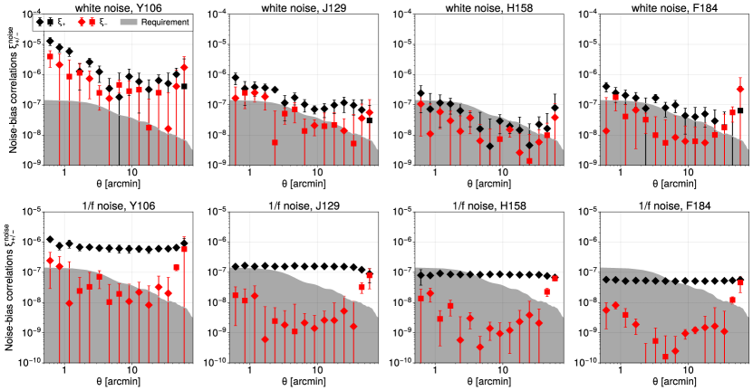
Figure 15: Auto-correlations of the noise bias ($\Delta g$) estimated with white noise (top) and 1/f (bottom) noise models for all the four bandpasses are shown. “diamond” marker is the positive signal while “square” is the negative signal but taken absolute value. These are normalized to single-epoch signal-to-noise ratio $\nu_{\rm SE}=10$ and (for the $1/f$ noise case) a knee frequency of $f_{\rm knee}=1$ kHz. Note that white noise biases generally scale as $\propto 1/\nu_{\rm SE}^{2}$ and $1/f$ noise biases scale as $\propto f_{\rm knee}/\nu_{\rm SE}^{2}$; this means that their correlation functions scale as $\propto 1/\nu_{\rm SE}^{4}$ and $\propto f_{\rm knee}^{2}/\nu_{\rm SE}^{4}$, respectively. These are the “raw” biases, with no attempt at mitigation.

5 Synthetic wide band images

Synthetic wide band images, created by stacking several standard-width filters, are often used as an intermediate product in weak lensing analyses (e.g., $r+i+z$ in DES (Dark Energy Survey Collaboration et al., 2018, 2021)). They can be used for making a deep detection image, or as a reference for forced photometry in individual filters for photometric redshifts. (This could include filters on other observatories, e.g., Vera Rubin Observatory data if one were to make a Y106+J129+H158+F184 image with Roman.) One could also make a shape catalog from the combined Y106+J129+H158+F184 imaging; such a catalog would have the advantages of providing a deeper catalog and reducing noise biases, but the disadvantage that with only one catalog using all the data one can only measure a shape auto-correlation (we would not have the option of cross-correlating two different versions of the shape catalog from different data). It is also possible that one would use both the single-band and the synthetic wide band shape catalogs to test for different systematics — for example, the individual bands allow for cross-correlations to test for PSF systematics associated with the tiling pattern (which is different in each filter; Spergel et al. 2015), but the wide-band image has lower noise bias.

We have built a set of wide band images in post-processing as follows. First, the output images in each filter $a$ are smoothed to a common output PSF $\Gamma_{\rm out}$ by convolving with a kernel $K_{a}$. Ideally, we want the coadd PSF $\Gamma_{a}$ convolved with this kernel to be the output PSF, $\Gamma_{a}\otimes K_{a}\approx\Gamma_{\rm out}$; in practice, we do this by writing

$$\tilde{K}_{a}({\mn@boldsymbol{u}})=\frac{\tilde{\Gamma}^{\ast}_{a}({\mn@boldsymbol{u}})\tilde{\Gamma}_{\rm out}({\mn@boldsymbol{u}})}{|\tilde{\Gamma}_{\rm out}({\mn@boldsymbol{u}})|^{2}+\epsilon^{2}}.$$ (20)

Without the $\epsilon$ term, this kernel would exactly transform the PSF $\Gamma_{a}$ into $\Gamma_{\rm out}$; but we set $\epsilon=10^{-4}$ in the denominator to avoid division by a near-zero quantity. The kernel is clipped to a $201\times 201$ output pixel region. We choose the output PSF $\Gamma_{\rm out}$ to be an Airy disc convolved with a Gaussian as in Paper I; the Airy disc parameters are $\lambda/D=0.112$ arcsec (the size for J129), obscuration 0.31, and the Gaussian has a scale length of $\sigma=0.1051$ arcsec (the largest of the Gaussian widths used in Paper I). The full width at half maximum of this output PSF is 0.287 arcsec.

Next, the images are added with some weights:

$$H_{\rm out}(x,y)=\sum_{a}w_{a}C_{a}\sum_{\Delta x,\Delta y}K_{a}(\Delta x,\Delta y)H_{a}(x-\Delta x,y-\Delta y),$$ (21)

where $H_{a}$ is the input image in band $a$, and $H_{\rm out}$ is the output image. The normalization factors $C_{a}$ convert the input units (electrons per $s_{\rm in}^{2}$ per exposure) into surface brightness units ($\mu$Jy $s_{\rm out}^{-2}$, or $\mu$Jy per output pixel) using the effective area curves provided by the Roman project. The weights (summing to $\sum_{a}w_{a}=1$) are proportional to the inverse square depths given by Akeson et al. (2019): 0.294, 0.323, 0.294, and 0.089 for the Y106, J129, H158, and F184 bands respectively. Examples of the synthetic wide images are shown in Fig. 16.

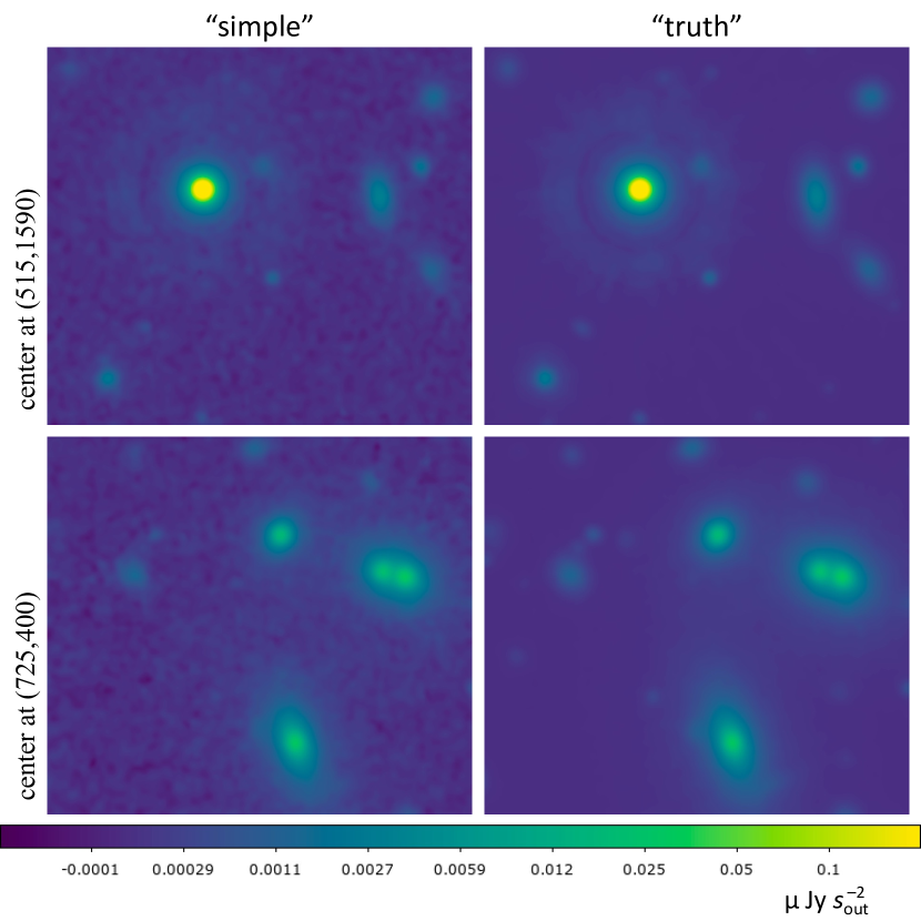
Figure 16: Two examples of fields in the synthetic wide band images (Sec. 5), from block (0,14). The left column shows the “simple” detector model, the right column shows “truth” (the noiseless image). The top row contains a bright star that saturates on the color scale (reaching 0.90 $\mu$Jy $s_{\rm out}^{-2}$ at its center), with a log stretch to show the wings of the output PSF. Both images show a $450\times 400$ output pixel ($11.25\times 10$ arcsec) region.

These images are then used again to extract stars to measure their properties, especially the two-point correlation functions. We measure the centroids and shapes of the stars using adaptive moments, and Figure 17 shows their shape-shape and shape-position correlation functions. Although these signals suggest that the star ellipticity correlations are within the requirement defined in SRD, we do not see an improvement in removing the residual contamination compared to the cases with individual bandpasses shown in Fig. 13.

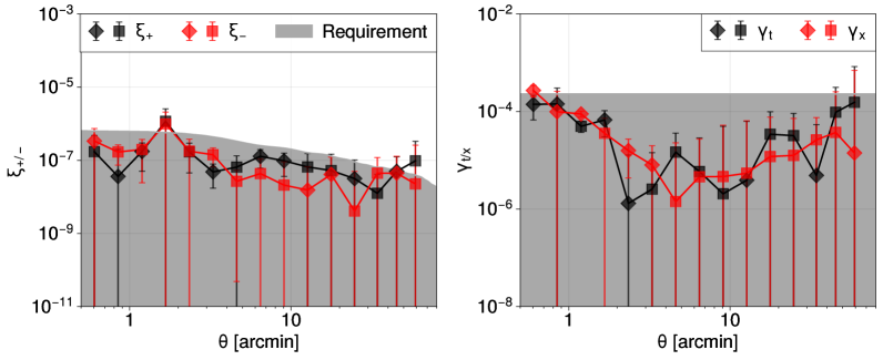
Figure 17: Shape-shape (Left) and shape-position (Right) correlation functions of stars observed in the synthetic wide band images. The grey region shows the estimated requirement on the signals from the PSF ellipticity additive error requirement in the SRD. “diamond” marker is the positive signal while “square” is the negative signal but taken absolute value.

6 Summary and Discussion

In this paper, we have analyzed the coadded images that are produced in Paper I. The layers that were simulated in Paper I include the simulated sky image produced in Troxel et al. (2023), the injected point sources ($\delta$-function convolved with Roman PSF), and two types of noise fields (white noise and 1/f noise). We have measured the following statistics on these images that are relevant to better characterize the weak lensing shear systematics:

• the power spectra of coadded white noise and $1/f$ noise, as measured in the output images;

• one point statistics of magnitude, astrometric error, 2nd moments (shape and size), and 4th order moments of the injected stars (an idealized case with no blending or chromaticity effects) and stars in the coadded sky image; and

• two-point statistics (shape-shape $\xi_{\pm}$ and position-shape $\gamma_{\rm t/x}$) of shapes and/or positions of the same sources.

If Roman images are to be processed using Imcom, it is essential to understand the implications of noise biasing on measurements of galaxy shapes. Noise power spectra are directly involved in the calculation of shape measurement bias (Appendix A), so we first investigated the power spectra of the coadded white and $1/f$ noise fields. In both cases, the noise power spectra of the coadded images decline to zero beyond $\sim 5$–6 cycles arcsec^-1, depending on the band. Specific features in the 2-dimensional and azimuthally averaged 1-dimensional power spectra indicate correlations in the noise fields that will impact shape measurements. We find that the most prominent features in the noise power spectra come from: band limits on the output PSFs, input image pixel positions, and the postage stamp boundaries and angular size. By comparing with analytic models of the expected 1-dimensional power spectra for well-sampled images (following derivations found in Appendix A), we recover some of the expected qualitative features, but the noise power spectra are generally above the simple expectation. This highlights the importance of using full simulations of the image processing steps to predict the output noise and associated biases, rather than using simple formulae appropriate for well-sampled data. Each filter performs slightly differently, with the increase in power spectrum relative to the simplistic expectation being worst in Y106. This is unsurprising since it has the worst coverage and sampling of all the filters (see Paper I for further discussion of coverage regions).

We have additionally presented the average astrometric offset from input catalog positions and the shape and size deviation from target PSF measured on injected stars (coadded PSF), and compared them to the PSF requirements documented in the Roman SRD. We have shown (Fig. 6) that they are well within the requirements in a root-mean-square sense in the four bandpasses in the Reference survey design (Y106, J129, H158, F184). The Imcom algorithm, although much more computationally expensive, has yielded large gains in output PSF quality relative to the current “industry standard” for combining space images (Drizzle).

Since what matters to weak lensing studies in the end is the level of contamination each systematic effect has in shape correlations, we have measured two-point correlation functions of shapes (2nd moments: Fig. 13) of the injected and simulated (sky image) stars and 4th order moments (Fig. 14) of injected stars. While the PSF shape-shape correlations are well below the mission requirement for all the bandpasses, the 4th moment-4th moment correlations in F184 is on the verge of falling short (other 4th moment correlations are not of concern).

We finally investigated the additive bias imprinted on the shapes of the injected stars by both white and $1/f$ noise in the input images, by adding the appropriate noise fields in and re-measuring the shapes. We find biases that exceed Roman requirements when scaled to signal-to-noise ratio per observation $\nu_{\rm SE}=10$, indicating that noise bias will have to be corrected in Roman analyses (as is already planned for Roman and other weak lensing projects). Appendix B develops an analytic model for the noise bias, which we find is in agreement with the observed trends.

While this set of simulations represents a major step toward use of the Imcom algorithm to the Roman weak lensing program, there are several more studies that should be carried out prior to implementation in an operational pipeline. These include:

• Computational efficiency: The existing implementation is computationally expensive, and would require $\sim 10^{9}$ CPU-hours to run on the full baseline HLIS survey if there were no speed-ups, whereas Drizzle would require $\sim 10^{5}$ CPU hours (extrapolated from the implementation in Troxel et al. 2023). On the algorithm side, one could investigate optimizing postage stamp and padding parameters (see Paper I), or re-arranging the linear algebra operations in Imcom if we can search over a limited range in the Lagrange multiplier $\kappa$. On the hardware/firmware side, one could make use of ongoing advances in graphics processing unit-accelerated linear algebra.

• Extended source injection: The tests with injected stars in this paper used point sources since these are a “stress test” for undersampling effects. However, we also want to implement grids of extended sources so that we can test Metacalibration (Huff & Mandelbaum, 2017; Sheldon & Huff, 2017) or analytic differentiation (Li & Mandelbaum, 2023) techniques wrapped around an algorithm that operates on an Imcom coadd.

• Error propagation: We would like to study propagation of astrometric errors, relative flux calibration between images, and PSF model errors through the image coaddition pipeline. This will involve the insertion of specialized layers with these types of errors injected.

• Laboratory noise fields: The analysis of the laboratory noise fields from this project, and an assessment of their implications for additive noise bias, is ongoing. Additional noise fields from the focal plane level and Wide Field Instrument level tests will be incorporated as they become available.

• Poisson noise bias corrections: While Imcom coaddition is a linear operation on the input pixels, shape measurement algorithms are non-linear operations on the data and hence are subject to noise biases. The current implementation allows one to coadd simulated noise relatizations, and therefore one can generate simulated output noise, as needed by tools such as Deep Metacalibration (Zhang et al., 2023a). Such realizations would also allow a Monte Carlo evaluation of the noise bias terms in twice-differentiable shape measurement algorithms (e.g., Li et al. 2022; Li & Mandelbaum 2023). The performance of the method has not been tested on simulations with source Poisson noise. But further work will be needed to address biases arising from self-Poisson noise of the source galaxies (e.g., Appendix D of Li & Mandelbaum, 2023).

• Chromatic effects: When running image combination in mosaic mode, one has to choose a “reference” intraband SED in order to have a well-defined PSF, but of course the sources in the field have a range of SEDs. Chromatic terms in the PSF will arise from diffraction, dispersion in the filter substrate, chromatic wavefront from mirror, filter, and detector coatings, and depth-dependent absorption effects in the detectors (Mosby et al., 2020). Additionally, there is a field-dependent filter bandpass due to angle of incidence effects, which results in objects redder than the reference SED having a normalization that is larger for input exposures near the field center and smaller for input exposures near the corners of the field. We plan to test how these chromatic effects propagate through Imcom and assess how they should be corrected.

• Deep fields: Like other weak lensing surveys, the Roman HLIS requires deep fields for photo-$z$, selection, and noise bias calibration. Some shear calibration algorithms also require deep fields (Zhang et al., 2023a). The Imcom algorithm will run on deep fields, but since the current version has ${\mathcal{O}}(n^{3})$ (where $n$ is the number of input pixels), a deep survey with $10$ as many exposures but only 1% of the area of the wide survey actually requires $10^{3}\times 0.01=10$ times as many operations to run Imcom as the wide survey if done by brute force. One solution to mitigate this is to coadd subsets of the deep field exposures to obtain full sampling at a common PSF, and then do a pixel-by-pixel coadd, but other options should be investigated for feasibility and performance. Another opportunity for the deep fields, since the observations include large dithers, would be to mitigate field-dependent bandpass effects. This would involve extending the linear algebra formalism in Rowe et al. (2011) to simultaneously reconstruct both an image through the “mean” bandpass in each filter and a “first principal component” (PC1) bandpass.

• Other survey strategies: The Reference survey strategy was developed to support hardware trades for the Roman mission, and the actual survey design may be different (see, e.g., Eifler et al. 2021 for one proposal). Simulations similar to those in this series of papers should be carried out for the possible alternative survey designs to ensure the data will be usable.

Data Availability

The codes for this project, along with sample configuration files and setup instructions, are available in the two GitHub repositories:

• https://github.com/hirata10/furry-parakeet.git (postage stamp coaddition)

• https://github.com/hirata10/fluffy-garbanzo.git (mosaic driver)

The version of the code used for this project is in tag 0.1.

Appendix A Models for the output noise power spectra in the absence of sampling effects

This appendix derives the analytic predictions for output noise power spectra in the absence of sampling effects, as used in Section 3. There are two cases for the input noise: white noise, and $1/f$ noise.

A.1 Input white noise

To calculate the expected output power spectrum for white noise, we start by writing the input and output images ({$I_{a}\}_{a=0}^{N_{\rm in}-1}$ and $H_{\rm out}$) as convolutions of the input and output PSFs $G_{\rm in}$ and $\Gamma_{\rm out}$ with the sky scene $f({\mn@boldsymbol{r}})$:

$$I_{a}(\vec{r})=[G_{\rm in}\ast f]({\mn@boldsymbol{r}}){\rm~{}~{}and~{}~{}}H_{\rm out}({\mn@boldsymbol{r}})=[\Gamma_{\rm out}\ast f]({\mn@boldsymbol{r}}).$$ (22)

where the input PSF $G_{\rm in}$ is the Airy disc convolved with a top hat function, $a$ is the index of the input PSF, and the target PSF $\Gamma_{\rm out}$ is the Airy disc convolved with a Gaussian. Taking the Fourier transform and combining these equations for each input image $j$ gives:

$$\tilde{H}_{{\rm out}}=\frac{\tilde{\Gamma}_{\rm out}({\boldsymbol{\upsilon}})}{\tilde{G}_{\rm in}({\boldsymbol{\upsilon}})}\sum_{j=0}^{N_{\rm in}-1}\frac{\tilde{I}_{a,j}({\boldsymbol{\upsilon}})}{N_{\rm in}},$$ (23)

where ${\boldsymbol{\upsilon}}=(u,v)$ is the wave vector. For independent input images, the power spectrum of the output is

$${P}_{\rm out}(\vec{k})=\Bigg{|}\frac{\tilde{\Gamma}_{\rm out}({\boldsymbol{\upsilon}})}{\tilde{G}_{\rm in}({\boldsymbol{\upsilon}})}\Bigg{|}^{2}\frac{{P}_{\rm in}({\boldsymbol{\upsilon}})}{N_{\rm in}}.$$ (24)

Here the Airy disc components of the PSFs cancel each other out when we take the ratio $\tilde{\Gamma}_{\rm out}/\tilde{G}_{\rm in}$, so this ratio is simply the ratio of the Gaussian to the sinc (Fourier transform of the top-hat). Following numpy convention and Paper I, we use the definition of the sinc function ${\rm sinc}(\xi)=\sin{\pi\xi}/\pi\xi=j_{0}(\pi\xi)$, where $j_{0}$ is the zeroth order spherical Bessel function. Then

$${P}_{\rm out}({\boldsymbol{\upsilon}})=\Bigg{|}\frac{{\rm e}^{-2\pi^{2}\sigma^{2}\upsilon^{2}}}{\text{sinc}(s_{\rm in}u)\,\text{sinc}(s_{\rm in}v)}\Bigg{|}^{2}\frac{P_{\rm in}({\boldsymbol{\upsilon}})}{N_{\rm in}}.$$ (25)

In this case, we are interested in input white noise with unit variance in pixels of area $s_{\rm in}^{2}$, so the input power spectrum is $P_{\rm in}({\boldsymbol{\upsilon}})=s_{\rm in}^{2}$.

We now taking an angular average over the direction of the Fourier mode $\varphi\in[0,2\pi)$ at fixed magnitude $\upsilon$. In this case, $u=\upsilon\cos\varphi$ and $v=\upsilon\sin\varphi$. After a lengthy but straightforward calculation, we get

$$\Big{\langle}{P}_{\rm out}({\boldsymbol{\upsilon}})\Big{\rangle}_{\varphi}=\frac{s_{\rm in}^{2}}{N_{\rm in}}\text{exp}\left[4\pi^{2}\left(\frac{s_{\rm in}^{2}}{12}-\sigma^{2}\right)\upsilon^{2}-\frac{\pi^{4}}{120}s_{\rm in}^{4}\upsilon^{4}+...\right],$$ (26)

where the “…” denote higher terms in the Taylor expansion of $\upsilon$. Note that the power spectrum has units of area since it is of an input field that is dimensionless by construction. This is the analytic expectation for the white noise power spectrum used in the analysis in Section 3 in this work.

A.2 Input $1/f$ noise

We now consider the case of input $1/f$ noise. To avoid clutter, we work initially in units of the input pixel scale (up through Eq. 41), and then transform units at the end.

The input $1/f$ noise fields are generated as 1D time-ordered data (TOD), and re-formatted into a 2D image. Thus for the prediction of an output noise power spectrum for input $1/f$ noise, we start with the power spectrum as a function of frequency on the 1D pixel axis,

$$P_{\rm TOD}(f)=\begin{cases}\frac{1}{2|f|}&\text{if }\frac{1}{N^{2}}<|f|<\frac{1}{2}\\ 0&\text{otherwise}\end{cases},$$ (27)

where $\frac{1}{2}$ is the Nyquist frequency (in units where the time to sample each pixel is unity) and $1/N^{2}$ is the cutoff for a sequence of $N^{2}$ pixels. Any two pixels separated by some time $t$ have a correlation function

$$\xi_{\rm TOD}(t)=\int P_{\rm TOD}(f)e^{2\pi\,{\rm i}ft}\,{\rm d}f=\int_{f_{min}}^{1/2}\frac{1}{f}\cos(2\pi\,ft)\,{\rm d}f,$$ (28)

where we have substituted $P_{\rm TOD}(f)$, used the fact that the $f<0$ range contributes the conjugate of the $f>0$ range, and set $f_{max}=1/2$ (the Nyquist frequency).

Pixels separated by $t$ in the time series are separated by some $(\Delta x,\Delta y)$ in the input data. The 1D (TOD) and 2D correlation functions are thus of the form $\xi_{\rm 2D}(\Delta x,\Delta y)$ and $\xi_{\rm TOD}(\Delta x+N\Delta y)$. Summing over $(\Delta x,\Delta y)$ gives us a 2D power spectrum (in Fourier space):

$${P}_{\rm 2D}(u,v) = \sum_{\Delta x,\Delta y}\xi_{\rm 2D}(\Delta\,x,\Delta\,y)e^{2\pi\,{\rm i}(u\Delta x+v\Delta y)}$$ (29)

$$= \sum_{\Delta x,\Delta y}\xi_{\rm TOD}(\Delta x+N\Delta y)e^{2\pi\,{\rm i}(u\Delta x+v\Delta y)}$$

$$= \sum_{\Delta y}e^{2\pi{\rm i}v\Delta y}\Big{[}\sum_{\Delta x}\xi_{\rm TOD}(\Delta x+N\Delta y)$$

$$~{}~{}~{}~{}\times e^{2\pi\,{\rm i}u(\Delta x+N\Delta y)}\Big{]}e^{-2\pi\,{\rm i}uN\Delta y}.$$

In the last line we have factored out an exponential so that we may substitute, in analogy with the first line,

$${P}_{\rm TOD}(u)=\sum_{\Delta x}\xi_{\rm TOD}(\Delta x+N\Delta y)e^{2\pi{\rm i}u(\Delta x+N\Delta y)}.$$ (30)

This gives the 2D power spectrum of the image as a function of the 1D power spectrum of the time-ordered data:

$${P}_{\rm 2D}(u,v)=\sum_{\Delta y}e^{2\pi{\rm i}v\Delta y}P_{\rm TOD}(u)e^{-2\pi{\rm i}uN\Delta y},$$ (31)

which, using the exponential form definition of the -function $\Sha(x)=\sum_{n=-\infty}^{\infty}e^{2\pi{\rm i}nx}$ (the “Shah” or Dirac Comb function), becomes:

$${P}_{\rm 2D}(u,v)=\Sha(v-uN)\tilde{P}_{\rm TOD}(u).$$ (32)

Equation (32) is general in the case that one considers the full plane, extending to infinity. However, the presence of the -function (and hence $\delta$-function) presents a challenge to numerical computation. The solution is to “smear out” the $\delta$-function according to the uncertainty principle given that our detector array is finite in size. In a finite region, the measured power spectrum ${P}_{\rm meas}({\boldsymbol{\upsilon}})$ is related to the true power spectrum ${P}({\boldsymbol{\upsilon}})$ by

$${P}_{\rm meas}({\boldsymbol{\upsilon}})=\frac{1}{A}\int\,{\rm d}^{2}{\boldsymbol{\upsilon}}^{\prime}{P}({\boldsymbol{\upsilon}})|\tilde{W}({\boldsymbol{\upsilon}}-{\boldsymbol{\upsilon}}^{\prime})|^{2},$$ (33)

where $A$ is the area of the space and $\tilde{W}$ is the window function (Fourier transform of the region measured; see discussion in Section 13.4 of Press et al. 1992).

We consider a rectangle of width $N$ (in the $x$-direction) and $N_{y}$ (in the $y$-direction) gives $A=NN_{y}$ and a window function

$$|\tilde{W}(\Delta u,\Delta v)|^{2}\!\!\!\! = \!\!\!\!(NN_{y})^{2}\,{\rm sinc}^{2}(N\Delta u)\,{\rm sinc}^{2}(N_{y}\Delta v)$$ (34)

$$\approx \!\!\!\!{\rm sinc}^{2}(N\Delta u)\,N^{2}N_{y}\delta(\Delta\,v).$$

Applying this to our 2D power spectrum for $1/f$ noise gives

$${P}_{\rm 2D,meas}(u,v) = \frac{1}{NN_{y}}\int\,{\rm d}\Delta u\,{\rm d}\Delta v\,\Sha(v^{\prime}-u^{\prime}N){P}_{\rm TOD}(u^{\prime})$$ (35)

$$~{}~{}~{}~{}\times{\rm sinc}^{2}(N\Delta u)\,N^{2}N_{y}\delta(\Delta\,v)\text{ },$$

where we have defined $u^{\prime}=u-\Delta u$ and $v^{\prime}=v-\Delta v$. Performing the integral over $\Delta v$ thus takes $v^{\prime}\rightarrow v$, resulting in

$${P}_{\rm 2D,meas}(u,v)\!\!\!\! = \!\!\!\!N\int{\rm d}\Delta u\,\Sha(v-uN+N\Delta u)$$ (36)

$$~{}~{}~{}~{}\times{P}_{\rm TOD}(u-\Delta u)\,{\rm sinc}^{2}(N\Delta u).~{}~{}~{}~{}$$

The -function can equivalently be written as $\Sha(x)=\sum_{n=-\infty}^{\infty}\delta(x-n)$, which will allow us to trivially perform the integral over $\Delta u$ as well:

$${P}_{\rm 2D,meas}(u,v)=\sum_{j=-\infty}^{\infty}{P}_{\rm TOD}\left(\frac{v-j}{N}\right)\,{\rm sinc}^{2}(Nu+j-v).$$ (37)

Finally, we substitute in our time-ordered power spectrum given for $1/f$ noise, Eq. (27), and find that the measured power spectrum for $1/f$ noise should be

$${P}_{\rm 2D,meas}(u,v)=\frac{N}{|v-j|}\,{\rm sinc}^{2}(Nu+j-v).$$ (38)

To include this result in our 1D representations in Figure 4, we convert to polar coordinates $\upsilon=\sqrt{u^{2}+v^{2}}$ and $\varphi=\,{\rm arctan2}(v,u)$, and take the angular average:

$$\left\langle{P}_{\rm 2D,meas}(\upsilon,\varphi)\right\rangle_{\varphi}\!\!\!\! = \!\!\!\!\int_{0}^{2\pi}\frac{{\rm d}\varphi}{2\pi}\sum_{j=-\infty}^{\infty}{P}_{\rm TOD}\left(\frac{\upsilon\sin\varphi-j}{N}\right)$$ (39)

$$\times{\rm sinc}^{2}(N\upsilon\cos\varphi+j-\upsilon\sin\varphi).$$

We can restrict the range of $j$ since the TOD power spectrum has a Nyquist frequency, so we include only

$$\frac{-1}{2}<\frac{r\sin\varphi-j}{N}<\frac{1}{2}.$$ (40)

The integral can be turned into a sum using $\varphi=2\pi\,K_{\varphi}/N_{\varphi}$, resulting in the final form we use to compute the expectations for the 1D $1/f$ noise power spectra:

$${P}_{\rm meas,2D\,ang.\,ave.}(\upsilon)\!\!\!\! = \!\!\!\!\frac{1}{N_{\varphi}}\sum_{K_{\varphi}=0}^{N_{\varphi}-1}\sum_{j=j_{\rm min}}^{j_{\rm max}}{P}_{\rm TOD}\left(\frac{\upsilon\sin\varphi-j}{N}\right)$$ (41)

$$\times\,{\rm sinc}^{2}(N\upsilon\cos\varphi+j-\upsilon\sin\varphi).$$

We note that this is in a single input image, in units where $s_{\rm in}=1$. To compare to the power spectra in Sec. 3.3, we must convert back to general units, include the factor of $1/N_{\rm in}$ for the input exposures, and include the square of ratios of modulation transfer functions to convert to the output images (as in Eq. 26). The result is

$$\Big{\langle}{P}_{\rm out}({\boldsymbol{\upsilon}})\Big{\rangle}_{\varphi}\!\!\!\! = \!\!\!\!\frac{1}{N_{\varphi}}\sum_{K_{\varphi}=0}^{N_{\varphi}-1}\sum_{j=j_{\rm min}}^{j_{\rm max}}{P}_{\rm TOD}\left(\frac{s_{\rm in}\upsilon\sin\varphi-j}{N}\right)$$

$$\times\,{\rm sinc}^{2}(Ns_{\rm in}\upsilon\cos\varphi+j-s_{\rm in}\upsilon\sin\varphi)$$

$$\times\frac{s_{\rm in}^{2}}{N_{\rm in}}\text{exp}\left[4\pi^{2}\left(\frac{s_{\rm in}^{2}}{12}-\sigma^{2}\right)\upsilon^{2}-\frac{\pi^{4}}{120}s_{\rm in}^{4}\upsilon^{4}+...\right].$$

We use $N=128$ as the width of the output channels (Mosby et al., 2020).

Appendix B Additive bias from anisotropic noise

While we have used injected stars with and without noise added to estimate the additive noise bias in the main text of the paper (Section 4.5), it is useful to have an analytic model in order to understand the orders of magnitude in the problem and the scaling behaviors. These analytic models, once calibrated with simulations, are also useful for setting requirements on knowledge of correlated noise — in particular, they were used to determine how many dark images needed to be taken at each calibration epoch to measure read noise correlations in the Roman Design Reference Mission. The main objective of this appendix is to predict the additive bias $c$ for ellipticity of stars or of galaxies in terms of the noise power spectrum $P_{\rm N}(u,v)$. For simplicity, this appendix does so for the adaptive moments method (Bernstein & Jarvis, 2002). A related previous study on noise biases in fitting elliptical Gaussians can be found in Condon (1997).

We follow the description of biases in Appendix C of Hirata et al. (2004) and Appendix A of Refregier et al. (2012). This description applies to the biases in a least-squares fitting algorithm where the galaxy image $I({\mn@boldsymbol{x}})$ is fit by a model $J({\mn@boldsymbol{x}}|{\mn@boldsymbol{p}})$, where ${\mn@boldsymbol{p}}$ is a point in a parameter space with parameters $\{p^{\alpha}\}$ (with $N$ parameters). The metric for the least-squares fit is assumed to be an inner product, denoted by $\langle,\rangle$: that is, the “energy functional” that is minimized is

$$E=\langle I-J({\mn@boldsymbol{p}}),I-J({\mn@boldsymbol{p}})\rangle=\frac{1}{2}\int|I({\mn@boldsymbol{x}})-J({\mn@boldsymbol{x}}|{\mn@boldsymbol{p}})|^{2}\,d^{2}{\mn@boldsymbol{x}}.$$ (43)

This definition guarantees the functional derivative

$$\frac{\delta}{\delta g({\mn@boldsymbol{x}})}\langle f,g\rangle=f({\mn@boldsymbol{x}}).$$ (44)

We assume we are working with a well-sampled image (in the context of this paper, that means the output image generated by Imcom) so that summations over pixels instead of integrals, and hence partial instead of functional derivatives, may also be used. The case considered here is more difficult than that in Hirata et al. (2004), because in the Hirata et al. (2004) calculation the least squares fit is inverse-noise-weighted with respect to the true noise covariance matrix. In contrast, here we are interested in the case where the true noise covariance is not the weight used in the inner product of Eq. (43). Indeed, the true noise covariance may not be known exactly, and one of our purposes is to understand what impact errors in the noise model have on output shape measurements.

We further use subscripts on $J$ to indicate partial derivatives with respect to $p^{\alpha}$, and drop the arguments unless explicitly required for clarity: thus $J_{\alpha}=\partial J({\mn@boldsymbol{x}}|{\mn@boldsymbol{p}})/\partial p^{\alpha}$.

We first consider the general calculation of mean shifts and biases, and then proceed to the case of galaxy ellipticity.

B.1 General results

We note that the minimization of $E$ with respect to a parameter $p^{\alpha}$ leads to the minimization equation:

$$0=\frac{1}{2}\frac{\partial E}{\partial p^{\alpha}}=\langle I-J,J_{\alpha}\rangle.$$ (45)

This is a set of $N$ nonlinear equations for the $N$ parameters $\{p^{\alpha}\}_{\alpha=0}^{N-1}$ in terms of the image $I$. Clearly if $I=J({\mn@boldsymbol{P}})$ for some point ${\mn@boldsymbol{P}}$ in parameter space, then the solution to Eq. (45) is that $p^{\alpha}=P^{\alpha}$.

This solution can be Taylor-expanded. We must first take the functional derivative of Eq. (45) with respect to the image:

$$0=J_{\alpha}({\mn@boldsymbol{r}})+\left[-\langle J_{\beta},J_{\alpha}\rangle+\langle I-J,J_{\alpha\beta}\rangle\right]\frac{\delta p^{\beta}}{\delta I({\mn@boldsymbol{r}})},$$ (46)

and then one more derivative:

$$0 = J_{\alpha\beta}({\mn@boldsymbol{r}})\frac{\delta p^{\beta}}{\delta I({\mn@boldsymbol{s}})}+\Bigl{[}-\langle J_{\beta\gamma},J_{\alpha}\rangle-\langle J_{\beta},J_{\alpha\gamma}\rangle-\langle J_{\gamma},J_{\alpha\beta}\rangle$$ (47)

$$+\langle I-J,J_{\alpha\beta\gamma}\rangle\Bigr{]}\frac{\delta p^{\beta}}{\delta I({\mn@boldsymbol{r}})}\frac{\delta p^{\gamma}}{\delta I({\mn@boldsymbol{s}})}+J_{\alpha\beta}({\mn@boldsymbol{s}})\frac{\delta p^{\beta}}{\delta I({\mn@boldsymbol{r}})}$$

$$+\left[-\langle J_{\beta},J_{\alpha}\rangle+\langle I-J,J_{\alpha\beta}\rangle\right]\frac{\delta^{2}p^{\beta}}{\delta I({\mn@boldsymbol{r}})\delta I({\mn@boldsymbol{s}})}.$$

If we focus next on expanding around the point where $I=J$, then — defining ${H}^{\alpha\beta}$ to be the $N\times N$ matrix inverse of the symmetric matrix $\langle J_{\beta},J_{\alpha}\rangle$ — we find

$$\frac{\delta p^{\alpha}}{\delta I({\mn@boldsymbol{r}})}=H^{\alpha\beta}J_{\beta}({\mn@boldsymbol{r}})$$ (48)

and (after some simplification)

$$\frac{\delta^{2}p^{\beta}}{\delta I({\mn@boldsymbol{r}})\delta I({\mn@boldsymbol{s}})} = H^{\alpha\beta}H^{\gamma\delta}\frac{\partial}{\partial p^{\alpha}}\left[J_{\delta}({\mn@boldsymbol{r}})J_{\gamma}({\mn@boldsymbol{s}})\right]$$ (49)

$$-\left[\langle J_{\delta\gamma},J_{\alpha}\rangle+\langle J_{\delta},J_{\alpha\gamma}\rangle+\langle J_{\gamma},J_{\alpha\delta}\rangle\right]$$

$$\times H^{\alpha\beta}H^{\gamma\epsilon}H^{\delta\zeta}J_{\epsilon}({\mn@boldsymbol{r}})J_{\zeta}({\mn@boldsymbol{s}}).$$

Now we suppose that there is some noise covariance matrix ${\textbf{{N}}}({\mn@boldsymbol{r}},{\mn@boldsymbol{s}})=\langle\Delta I({\mn@boldsymbol{r}})\Delta I({\mn@boldsymbol{s}})\rangle$. Then let us define the symmetric matrix

$$Q_{\epsilon\zeta}\!\!\!\! = \!\!\!\!\int J_{\epsilon}({\mn@boldsymbol{r}})J_{\zeta}({\mn@boldsymbol{s}}){\textbf{{N}}}({\mn@boldsymbol{r}},{\mn@boldsymbol{s}})\,{\rm d}^{2}{\mn@boldsymbol{r}}\,{\rm d}^{2}{\mn@boldsymbol{s}}$$ (50)

$$= \!\!\!\!\int\tilde{J}^{\ast}_{\epsilon}({\boldsymbol{\upsilon}})\tilde{J}_{\zeta}({\boldsymbol{\upsilon}})P_{N}({\boldsymbol{\upsilon}})\,d^{2}{\boldsymbol{\upsilon}},$$

where $P_{\rm N}({\boldsymbol{\upsilon}})$ is the noise power spectrum at wave vector ${\boldsymbol{\upsilon}}=(u,v)$.

The covariance of the model parameters, from Eq. (48), is then

$${\rm Cov}(p^{\alpha},p^{\beta})=H^{\alpha\gamma}H^{\beta\delta}Q_{\gamma\delta},$$ (51)

and the bias is

$$\Delta p^{\beta}=\frac{1}{2}\int{\textbf{{N}}}({\mn@boldsymbol{r}},{\mn@boldsymbol{s}})\frac{\delta^{2}p^{\beta}}{\delta I({\mn@boldsymbol{r}})\delta I({\mn@boldsymbol{s}})}\,{\rm d}^{2}{\mn@boldsymbol{r}}\,{\rm d}^{2}{\mn@boldsymbol{s}}.$$ (52)

After simplifying using the idenitity (provable using the product rule)

$$\langle J_{\delta},J_{\alpha\gamma}\rangle+\langle J_{\gamma},J_{\alpha\delta}\rangle=\frac{\partial[{\textbf{{H}}}^{-1}]_{\gamma\delta}}{\partial p^{\alpha}},$$ (53)

this becomes

$$\Delta p^{\beta}=\frac{1}{2}H^{\alpha\beta}\left[\frac{\partial}{\partial p^{\alpha}}(H^{\gamma\delta}Q_{\gamma\delta})-\langle J_{\delta\gamma},J_{\alpha}\rangle H^{\gamma\epsilon}H^{\delta\zeta}Q_{\epsilon\zeta}\right],$$ (54)

where from Eq. (53):

$$\langle J_{\delta\gamma},J_{\alpha}\rangle=\frac{1}{2}\left(\frac{\partial[{\textbf{{H}}}^{-1}]_{\alpha\delta}}{\partial p^{\gamma}}+\frac{\partial[{\textbf{{H}}}^{-1}]_{\alpha\gamma}}{\partial p^{\delta}}-\frac{\partial[{\textbf{{H}}}^{-1}]_{\gamma\delta}}{\partial p^{\alpha}}\right).$$ (55)

Note the appearance of the bias tensor, as discussed in Cox & Snell (1968); this is very much like a Christoffel symbol if H is interpreted as a contravariant metric on parameter space. It appears in other contexts where we consider noise biases in photometry (e.g. Portillo et al., 2020). The first term, involving the derivative of $H^{\gamma\delta}Q_{\gamma\delta}$, does not appear in the usual formula for the bias of a maximum likelihood estimator; it results essentially from the fact that the weight in the inner product $\langle,\rangle$ used to define the energy functional $E$ is not an inverse-noise weighting with the true noise. In particular, one can show that for white noise with $P_{\rm N}({\boldsymbol{\upsilon}})=A$ that ${\textbf{{Q}}}=A{\textbf{{H}}}^{-1}$, and hence $\partial(H^{\gamma\delta}Q_{\gamma\delta})/\partial p^{\alpha}=0$. But it needs to be taken into account in the present context, where we allow an arbitrary noise power spectrum but then fit objects with uniform weighting.

Equation (54) is additive in the noise correlation function, as is always the case for second-order biases.

B.2 Application to ellipticities

We now consider the case where the particular model of interest is the fitting of an elliptical Gaussian:

$$J({\mn@boldsymbol{x}}|{\mn@boldsymbol{p}})=\frac{F}{2\pi\sqrt{\det\textbf{{M}}}}\exp\frac{-({\mn@boldsymbol{x}}-{\mn@boldsymbol{x}}_{\rm c})\cdot{\textbf{{M}}}^{-1}({\mn@boldsymbol{x}}-{\mn@boldsymbol{x}}_{\rm c})}{2},$$ (56)

where the parameters are the flux $F$, the centroid $(x_{c},y_{c})$, and the three moments of the $2\times 2$ symmetric matrix M, usually written in the form

$${\textbf{{M}}}=R^{2}\left(\begin{array}[]{cc}1+e_{1}&e_{2}\\ e_{2}&1-e_{1}\end{array}\right).$$ (57)

This is the Bernstein & Jarvis (2002) convention for ellipticities; the scale parameter $R$ was chosen to make M simple, and is defined in terms of the principal axes by $R^{2}=(a^{2}+b^{2})/2$. The Fourier transforms are

$$\tilde{J}({\boldsymbol{\upsilon}}|{\mn@boldsymbol{p}})=Fe^{-2\pi i{\mn@boldsymbol{x}}_{\rm c}\cdot{\boldsymbol{\upsilon}}}e^{-2\pi^{2}{\boldsymbol{\upsilon}}\cdot{\textbf{{M}}}{\boldsymbol{\upsilon}}}$$ (58)

(it is easiest to compute the inner products in Fourier space).

The derivatives of $J$ are

$$\tilde{J}_{F} = {\rm e}^{-2\pi{\rm i}{\boldsymbol{x}}_{\rm c}\cdot{\boldsymbol{\upsilon}}}{\rm e}^{-2\pi^{2}{\boldsymbol{\upsilon}}\cdot{\bf M}{\boldsymbol{\upsilon}}},$$

$$\tilde{J}_{x_{c}} = -2\pi{\rm i}uF{\rm e}^{-2\pi{\rm i}{\boldsymbol{x}}_{\rm c}\cdot{\boldsymbol{\upsilon}}}{\rm e}^{-2\pi^{2}{\boldsymbol{\upsilon}}\cdot{\bf M}{\boldsymbol{\upsilon}}},$$

$$\tilde{J}_{y_{c}} = -2\pi{\rm i}vF{\rm e}^{-2\pi{\rm i}{\boldsymbol{x}}_{\rm c}\cdot{\boldsymbol{\upsilon}}}{\rm e}^{-2\pi^{2}{\boldsymbol{\upsilon}}\cdot{\bf M}{\boldsymbol{\upsilon}}},$$

$$\tilde{J}_{R} = -\frac{4\pi^{2}}{R}{\boldsymbol{\upsilon}}\cdot{\bf M}{\boldsymbol{\upsilon}}F{\rm e}^{-2\pi{\rm i}{\boldsymbol{x}}_{\rm c}\cdot{\boldsymbol{\upsilon}}}{\rm e}^{-2\pi^{2}{\boldsymbol{\upsilon}}\cdot{\bf M}{\boldsymbol{\upsilon}}},$$

$$\tilde{J}_{e_{1}} = -2\pi^{2}R^{2}(u^{2}-v^{2})F{\rm e}^{-2\pi{\rm i}{\boldsymbol{x}}_{\rm c}\cdot{\boldsymbol{\upsilon}}}{\rm e}^{-2\pi^{2}{\boldsymbol{\upsilon}}\cdot{\bf M}{\boldsymbol{\upsilon}}},{\rm~{}~{}and}$$

$$\tilde{J}_{e_{2}} = -4\pi^{2}R^{2}uvF{\rm e}^{-2\pi{\rm i}{\boldsymbol{x}}_{\rm c}\cdot{\boldsymbol{\upsilon}}}{\rm e}^{-2\pi^{2}{\boldsymbol{\upsilon}}\cdot{\bf M}{\boldsymbol{\upsilon}}}.$$ (59)

These lead to the inverse matrix of inner products (where $e^{2}=e_{1}^{2}+e_{2}^{2}$ and $\xi=1-e^{2}$, and we have used many applications of Wick’s theorem):

H $$= \!\!\!\!4\pi R^{2}\sqrt{1-e^{2}}$$ (66)

$$\!\!\!\!\!\!\!\!\!\!\!\!\!\!\!\times\left(\!\begin{array}[]{cccccc}2&0&0&\frac{R}{F}&0&0\\ 0&\!\!\frac{2R^{2}(1+e_{1})}{F^{2}}\!\!&\frac{2R^{2}e_{2}}{F^{2}}&0&0&0\\ 0&\frac{2R^{2}e_{2}}{F^{2}}&\!\!\frac{2R^{2}(1-e_{1})}{F^{2}}\!\!&0&0&0\\ \frac{R}{F}&0&0&\frac{R^{2}(1+e^{2})}{F^{2}}&\frac{2R\xi e_{1}}{F^{2}}&\frac{2R\xi e_{2}}{F^{2}}\\ 0&0&0&\frac{2R\xi e_{1}}{F^{2}}&\!\!\frac{4\xi(1-e_{1}^{2})}{F^{2}}\!\!&\frac{-4\xi e_{1}e_{2}}{F^{2}}\\ 0&0&0&\frac{2R\xi e_{2}}{F^{2}}&\frac{-4\xi e_{1}e_{2}}{F^{2}}&\!\!\frac{4\xi(1-e_{2}^{2})}{F^{2}}\!\!\\ \end{array}\!\right).$$

From Eq. (50), the noise correlations projected into the data space can be written as an integral over the noise power spectrum:

$${\textbf{{Q}}}=\int{\boldsymbol{\tau}}{\boldsymbol{\tau}}^{\dagger}e^{-4\pi^{2}{\boldsymbol{\upsilon}}\cdot{\textbf{{M}}}{\boldsymbol{\upsilon}}}P_{N}(u,v)\,{\rm d}u\,{\rm d}v,$$ (68)

where the column vector ${\boldsymbol{\tau}}$ is a function of ${{\boldsymbol{\upsilon}}}$:

$${\boldsymbol{\tau}}=\left(\begin{array}[]{c}1\\ -2\pi{\rm i}Fu\\ -2\pi{\rm i}Fv\\ -4\pi^{2}RF[(1+e_{1})u^{2}+2e_{2}uv+(1-e_{1})v^{2}]\\ -2\pi^{2}R^{2}F(u^{2}-v^{2})\\ -4\pi^{2}R^{2}Fuv\end{array}\right).$$ (69)

We also need to use Eq. (55) to evaluate $\langle J_{\gamma\delta},J_{e_{1}}\rangle$ at zero ellipticity:

$$\langle J_{\gamma\delta},J_{e_{1}}\rangle|_{e=0}=\frac{1}{8\pi R^{2}}\left(\begin{array}[]{cccccc}0&0&0&0&\frac{F}{2}&0\\ 0&\frac{F^{2}}{2R^{2}}&0&0&0&0\\ 0&0&-\frac{F^{2}}{2R^{2}}&0&0&0\\ 0&0&0&0&-\frac{F^{2}}{2R}&0\\ \frac{F}{2}&0&0&-\frac{F^{2}}{2R}&0&0\\ 0&0&0&0&0&0\\ \end{array}\right).$$ (70)

After a tedious calculation, we find that the total ellipticity bias is

$$\Delta e_{1}\!\! = \!\!-\frac{256\pi^{4}R^{6}}{F^{2}}\int[4\pi^{2}(u^{2}+v^{2})R^{2}-1]^{2}(u^{2}-v^{2})$$ (71)

$$~{}\times{\rm e}^{-4\pi^{2}R^{2}(u^{2}+v^{2})}\,P_{\rm N}(u,v)\,{\rm d}u\,{\rm d}v.$$

An analogous equation holds for $\Delta e_{2}$:

$$\Delta e_{2}\!\! = \!\!-\frac{256\pi^{4}R^{6}}{F^{2}}\int[4\pi^{2}(u^{2}+v^{2})R^{2}-1]^{2}(2uv)$$ (72)

$$~{}\times{\rm e}^{-4\pi^{2}R^{2}(u^{2}+v^{2})}\,P_{\rm N}(u,v)\,{\rm d}u\,{\rm d}v.$$

The combined equation can be written in the form:

$$(\Delta e_{1},\Delta e_{2})=-\frac{R^{4}}{F^{2}}\int W(\upsilon R)(\cos 2\varphi,\sin 2\varphi)\,P_{\rm N}(u,v)\,{\rm d}u\,{\rm d}v,$$ (73)

where $\varphi=\arctan(v/u)$ is the position angle of mode $(u,v)$, $P_{\rm N}(u,v)\,{\rm d}u\,{\rm d}v$ is the differential contribution to the noise intensity variance $\sigma_{I}^{2}$, and the function

$$W(z)=256\pi^{4}z^{2}(4\pi^{2}z^{2}-1)^{2}{\rm e}^{-4\pi^{2}z^{2}}$$ (74)

is a dimensionless weight. The weight function goes to zero both at $z\rightarrow 0$ and $z\rightarrow\infty$: this is because correlated noise at zero spatial frequency is equivalent to an overall “pedestal” in the background at each galaxy, which may affect the flux measurement but does not bias the ellipticity. Noise at high spatial frequency $\upsilon\gtrsim 0.6/R$ is outside the band limit of the shape measurement, and hence has no effect.

Figure 18: The weight function $W(z)$ in Eq. (73) as a function of wave number. Note that an anisotropic contribution to the noise is most damaging at a scale of $\upsilon=\sqrt{u^{2}+v^{2}}\approx 0.3/R$ (or a wavelength of $\upsilon^{-1}\approx 3R$).

Note that the above considerations apply to the “as-observed” galaxy, e.g. “$R$” is the scale radius after convolution with the PSF, and $(\Delta e_{1},\Delta e_{2})$ is the noise-induced ellipticity bias before PSF correction. In e.g. a shape measurement method where the observed ellipticity is “corrected” by dividing by a responsivity factor ${\cal R}_{2}$ (usually between $\sim 0.3$ and 1), the bias on the reported ellipticity would also be divided by this factor. Also note that one must divide by 2 to get an ellipticity in the $g=(a-b)/(a+b)$ convention (where $a$ and $b$ are major and minor axes) instead of the $e=(a^{2}-b^{2})/(a^{2}+b^{2})$ convention:

$$(\Delta g_{1},\Delta g_{2})=-\frac{R^{4}}{2F^{2}}\int W(\upsilon R)(\cos 2\varphi,\sin 2\varphi)\,P_{\rm N}(u,v)\,{\rm d}u\,{\rm d}v.$$ (75)

The analytic formula is useful since it is applicable to any shape of the noise power spectrum: weakly anisotropic noise, “striping” noise (correlated in the row direction), and at any spatial scale. This allows us to rapidly estimate the order of magnitude of the bias introduced by a noise source, and understand its scaling behavior. However it is also critical to compare the analytic model to simulations.

B.3 Comparison to toy simulations

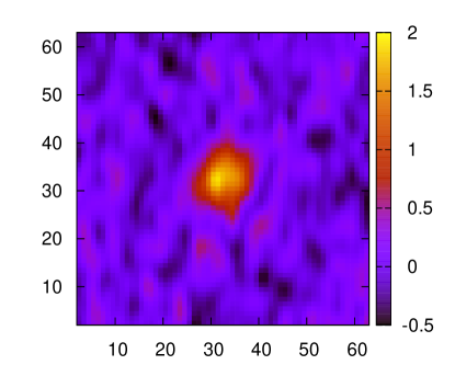
Figure 19: An example circular galaxy with flux $F=200$ counts and scale radius $R=4$ pixels, superposed on the noise field of Eq. (76) with $A=1$, $\alpha=4/\pi$, and $\beta=16/\pi$. That is, the correlation length of the noise is twice as large in the $y$-direction as the $x$-direction. Noise of this form leads to a bias of $e_{1}$ toward negative values, i.e., toward inferring a vertical orientation for the galaxy.

It is useful to compare the analytical bias estimate to a “toy” simulation designed to mimic the assumptions in the analytic model. This is a check of whether the analytical calculation is performed correctly, and also allows simple tests of its range of validity.

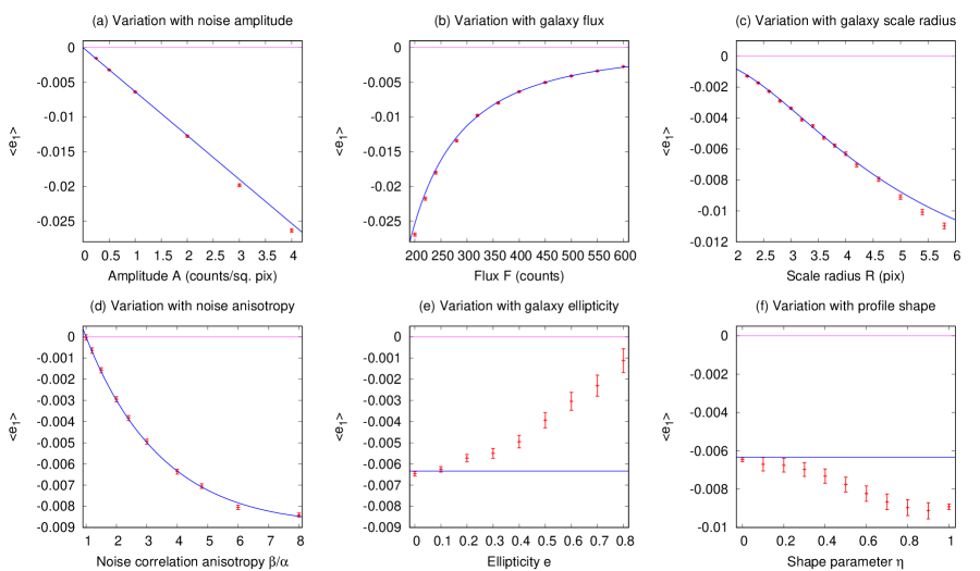
Figure 20: The shape measurement biases measured from simulations (red points with $1\sigma$ Monte Carlo errors) and calculated from the analytic approximation, Eq. (71) (blue lines). Each panel is based on the reference case (circular galaxy, $F=200$ counts, $R=4$ pixels, noise at $A=1$ with the noise spectrum of Eq. (76) except for the variations indicated. In panels (a–d), the agreement is in general excellent, but for small signal-to-noise ratio, statistically significant deviations can be seen. Panels (e) and (f) show cases that violate the assumptions of the analytic model, and hence show larger errors. The number of simulations per point is $10^{6}$, except for the $0<\eta<1$ points in panel (f), which are more computationally expensive; in these cases $10^{5}$ simulations were run.

The first set of such simulations is performed on a circular galaxy with flux $F=200$ counts, scale radius $R=4$ pixels, and centered at pixel $(32,32)$ of a $64\times 64$ simulation. A Gaussian random field was generated for the noise, with power spectrum:

$$P_{\rm N}(u,v)=A^{2}e^{-4\pi^{2}(\alpha u^{2}-\beta v^{2})},$$ (76)

where $A$ is an amplitude parameter (with units of counts per square pixel), and the default values of the constants are $\alpha=4/\pi$ and $\beta=16/\pi$. This results in a noise field correlated in the $y$ direction; see Figure 19.

We may now investigate the biases in ellipticity resulting from this noise field. We generated $10^{6}$ random realizations of the noise, and measured the galaxy shape each time using the least-squares elliptical Gaussian method. We compare the ellipticity bias with the analytical prediction of Eq. (71) for a range of galaxy parameters. For the noise spectrum of Eq. (76), the predicted bias can be obtained via integration over the Gaussian:

$$\Delta e_{1}\!\! = \!\!\frac{2\pi R^{6}A^{2}(\alpha-\beta)}{F^{2}(\alpha+R^{2})^{7/2}(\beta+R^{2})^{7/2}}\Bigl{[}28R^{8}+20(\alpha+\beta)R^{6}$$ (77)

$$+7(\alpha-\beta)^{2}R^{4}-4\alpha\beta(\alpha+\beta)R^{2}+4\alpha^{2}\beta^{2}\Bigr{]},$$

and this can be compared to the numerical results.

The outcome of these tests is shown in Figure 20. We see that, as expected, the noise bias scales as the noise variance $\propto A^{2}$ (panel a) and as the inverse square of the galaxy flux, $\propto 1/F^{2}$ (panel b). The radius dependence is more complex (panel c) — indeed, from Eq. (77), one can see that the bias approaches a constant at large $R$, i.e. when the size of the galaxy is large compared to the correlation length of the noise. This is because for fixed flux, the reduction in signal-to-noise as the light is spread over more pixels cancels against the decreasing importance of the noise correlations (since they are over a small fraction of a galaxy scale length). The noise anisotropy ($\beta/\alpha$, or aspect ratio squared) is varied in panel (d), with fixed $\alpha$. Good agreement with the analytical model is seen in all of these cases.

Panels (e) and (f) of Fig. 20 show effects not treated in the analytical model. In panel (e), we have varied the ellipticity of the galaxies — that is, instead of inserting a circular Gaussian galaxy, we have given it the indicated ellipticity $e=\sqrt{e_{1}^{2}+e_{2}^{2}}$ and assigned a random position angle $\chi=\frac{1}{2}\arctan(e_{2}/e_{1})$, and kept the same flux and scale radius $R$. It can be seen that for more elliptical galaxies, the bias becomes “smaller” (in absolute value, i.e. closer to zero).

Panel (f) shows the variation with the galaxy profile. For each value of $\eta$, a galaxy was generated via the convolution of an exponential profile and a Gaussian profile:

$$I=I_{\rm exp}\ast I_{\rm Gauss},~{}~{}~{}~{}I_{\rm exp}(r)\propto 2^{-r/r_{\rm e}},~{}~{}~{}~{}I_{\rm G}(r)\propto e^{-r^{2}/2r_{\rm G}^{2}},$$ (78)

and with a ratio of radii $r_{\rm e}:r_{\rm G}=\eta:1-\eta$. This interpolates between the pure Gaussian limit ($\eta=0$) and pure exponential ($\eta=1$). This is intended to be a crude representation of a centrally peaked galaxy with some smearing. The normalization (amplitude) and total radius are set so that the least-squares Gaussian fit has the default values of $F=200$ and $R=4$.

References

- Akeson et al. (2019) Akeson R., et al., 2019, arXiv e-prints, p. arXiv:1902.05569
- Albrecht et al. (2006) Albrecht A., et al., 2006, arXiv e-prints, pp astro–ph/0609591
- Astropy Collaboration et al. (2013) Astropy Collaboration et al., 2013, A&A, 558, A33
- Astropy Collaboration et al. (2018) Astropy Collaboration et al., 2018, AJ, 156, 123
- Astropy Collaboration et al. (2022) Astropy Collaboration et al., 2022, ApJ, 935, 167
- Bacon et al. (2001) Bacon D. J., Refregier A., Clowe D., Ellis R. S., 2001, MNRAS, 325, 1065
- Bernstein & Jarvis (2002) Bernstein G. M., Jarvis M., 2002, AJ, 123, 583
- Casey et al. (2023) Casey K. J., Greco J. P., Peter A. H. G., Davis A. B., 2023, MNRAS, 520, 4715
- Condon (1997) Condon J. J., 1997, PASP, 109, 166
- Cox & Snell (1968) Cox D. R., Snell E. J., 1968, J. Royal Stat. Soc., Series B, 30, 248
- Cropper et al. (2013) Cropper M., et al., 2013, MNRAS, 431, 3103
- Dark Energy Survey Collaboration et al. (2018) Dark Energy Survey Collaboration Abbott T. M. C., et al., 2018, ApJS, 239, 18
- Dark Energy Survey Collaboration et al. (2021) Dark Energy Survey Collaboration Abbott T. M. C., et al., 2021, ApJS, 255, 20
- Doré et al. (2018) Doré O., et al., 2018, arXiv e-prints, p. arXiv:1804.03628
- Eifler et al. (2021) Eifler T., et al., 2021, MNRAS, 507, 1514
- Erben et al. (2001) Erben T., Van Waerbeke L., Bertin E., Mellier Y., Schneider P., 2001, A&A, 366, 717
- Euclid Collaboration et al. (2020) Euclid Collaboration et al., 2020, A&A, 635, A139
- Finner et al. (2023) Finner K., Lee B., Chary R.-R., Jee M. J., Hirata C., Congedo G., Taylor P., HyeongHan K., 2023, ApJ, 958, 33
- Freudenburg et al. (2020) Freudenburg J. K. C., et al., 2020, PASP, 132, 074504
- Fruchter & Hook (2002) Fruchter A. S., Hook R. N., 2002, PASP, 114, 144
- Givans et al. (2022) Givans J. J., et al., 2022, PASP, 134, 014001
- Górski et al. (2005) Górski K. M., Hivon E., Banday A. J., Wandelt B. D., Hansen F. K., Reinecke M., Bartelmann M., 2005, ApJ, 622, 759
- Gurvich & Mandelbaum (2016) Gurvich A., Mandelbaum R., 2016, MNRAS, 457, 3522
- Harris et al. (2020) Harris C. R., et al., 2020, Nature, 585, 357
- Herbonnet et al. (2017) Herbonnet R., Buddendiek A., Kuijken K., 2017, A&A, 599, A73
- Heymans et al. (2006) Heymans C., et al., 2006, MNRAS, 368, 1323
- Hirata & Seljak (2003) Hirata C., Seljak U., 2003, MNRAS, 343, 459
- Hirata et al. (2004) Hirata C. M., et al., 2004, MNRAS, 353, 529
- Hoekstra et al. (2002) Hoekstra H., Yee H. K. C., Gladders M. D., 2002, New Astron. Rev., 46, 767
- Huff & Mandelbaum (2017) Huff E., Mandelbaum R., 2017, arXiv e-prints, p. arXiv:1702.02600
- Hunter (2007) Hunter J. D., 2007, Computing in Science & Engineering, 9, 90
- Ivezić et al. (2019) Ivezić Ž., et al., 2019, ApJ, 873, 111
- Jarvis et al. (2004) Jarvis M., Bernstein G., Jain B., 2004, MNRAS, 352, 338
- Jarvis et al. (2016) Jarvis M., et al., 2016, MNRAS, 460, 2245
- Jarvis et al. (2021) Jarvis M., et al., 2021, MNRAS, 501, 1282
- Joye & Mandel (2003) Joye W. A., Mandel E., 2003, in Payne H. E., Jedrzejewski R. I., Hook R. N., eds, Astronomical Society of the Pacific Conference Series Vol. 295, Astronomical Data Analysis Software and Systems XII. p. 489
- Jurić (2018) Jurić M., 2018, galfast: Milky Way mock catalog generator, Astrophysics Source Code Library, record ascl:1810.001 (ascl:1810.001)
- Jurić et al. (2008) Jurić M., et al., 2008, ApJ, 673, 864
- Kaiser (2000) Kaiser N., 2000, ApJ, 537, 555
- Kannawadi et al. (2021) Kannawadi A., Rosenberg E., Hoekstra H., 2021, MNRAS, 502, 4048
- Korytov et al. (2019) Korytov D., et al., 2019, ApJS, 245, 26
- Kovacs et al. (2022) Kovacs E., et al., 2022, The Open Journal of Astrophysics, 5, 1
- LSST Dark Energy Science Collaboration (LSST DESC) et al. (2021a) LSST Dark Energy Science Collaboration (LSST DESC) et al., 2021a, arXiv e-prints, p. arXiv:2101.04855
- LSST Dark Energy Science Collaboration (LSST DESC) et al. (2021b) LSST Dark Energy Science Collaboration (LSST DESC) et al., 2021b, ApJS, 253, 31
- LSST Science Collaboration et al. (2009) LSST Science Collaboration et al., 2009, arXiv e-prints, p. arXiv:0912.0201
- Laureijs et al. (2011) Laureijs R., et al., 2011, arXiv e-prints, p. arXiv:1110.3193
- Lemos et al. (2021) Lemos P., et al., 2021, MNRAS, 505, 6179
- Li & Mandelbaum (2023) Li X., Mandelbaum R., 2023, MNRAS, 521, 4904
- Li et al. (2022) Li X., Li Y., Massey R., 2022, MNRAS, 511, 4850
- Mandelbaum et al. (2005) Mandelbaum R., et al., 2005, MNRAS, 361, 1287
- Mandelbaum et al. (2015) Mandelbaum R., et al., 2015, MNRAS, 450, 2963
- Mandelbaum et al. (2023) Mandelbaum R., Jarvis M., Lupton R. H., Bosch J., Kannawadi A., Murphy M. D., Zhang T., 2023, The Open Journal of Astrophysics, 6, 5
- Massey et al. (2013) Massey R., et al., 2013, MNRAS, 429, 661
- Melchior & Viola (2012) Melchior P., Viola M., 2012, MNRAS, 424, 2757
- Mosby et al. (2020) Mosby G., et al., 2020, Journal of Astronomical Telescopes, Instruments, and Systems, 6, 046001
- Ohio Supercomputer Center (2018) Ohio Supercomputer Center 2018, Pitzer Supercomputer, http://osc.edu/ark:/19495/hpc56htp
- Oke & Gunn (1983) Oke J. B., Gunn J. E., 1983, ApJ, 266, 713
- Okura & Futamase (2018) Okura Y., Futamase T., 2018, MNRAS, 479, 4971
- Paulin-Henriksson et al. (2008) Paulin-Henriksson S., Amara A., Voigt L., Refregier A., Bridle S. L., 2008, A&A, 484, 67
- Paulin-Henriksson et al. (2009) Paulin-Henriksson S., Refregier A., Amara A., 2009, A&A, 500, 647
- Planck Collaboration et al. (2020) Planck Collaboration et al., 2020, A&A, 641, A6
- Portillo et al. (2020) Portillo S. K. N., Speagle J. S., Finkbeiner D. P., 2020, AJ, 159, 165
- Press et al. (1992) Press W. H., Teukolsky S. A., Vetterling W. T., Flannery B. P., 1992, Numerical recipes in C. The art of scientific computing. Cambridge University Press
- Rauscher (2015) Rauscher B. J., 2015, PASP, 127, 1144
- Refregier (2003) Refregier A., 2003, MNRAS, 338, 35
- Refregier et al. (2012) Refregier A., Kacprzak T., Amara A., Bridle S., Rowe B., 2012, MNRAS, 425, 1951
- Rowe et al. (2011) Rowe B., Hirata C., Rhodes J., 2011, ApJ, 741, 46
- Schneider & Seitz (1995) Schneider P., Seitz C., 1995, A&A, 294, 411
- Sheldon & Huff (2017) Sheldon E. S., Huff E. M., 2017, ApJ, 841, 24
- Sheldon et al. (2020) Sheldon E. S., Becker M. R., MacCrann N., Jarvis M., 2020, ApJ, 902, 138
- Spergel et al. (2015) Spergel D., et al., 2015, arXiv e-prints, p. arXiv:1503.03757
- The LSST Dark Energy Science Collaboration et al. (2018) The LSST Dark Energy Science Collaboration et al., 2018, arXiv e-prints, p. arXiv:1809.01669
- Troxel et al. (2021) Troxel M. A., et al., 2021, MNRAS, 501, 2044
- Troxel et al. (2023) Troxel M. A., et al., 2023, MNRAS, 522, 2801
- Weinberg et al. (2013) Weinberg D. H., Mortonson M. J., Eisenstein D. J., Hirata C., Riess A. G., Rozo E., 2013, Phys. Rep., 530, 87
- Yamamoto et al. (2023) Yamamoto M., Troxel M. A., Jarvis M., Mandelbaum R., Hirata C., Long H., Choi A., Zhang T., 2023, MNRAS, 519, 4241
- Zhang et al. (2023a) Zhang Z., Sheldon E. S., Becker M. R., 2023a, The Open Journal of Astrophysics, 6, 16
- Zhang et al. (2023b) Zhang T., et al., 2023b, MNRAS, 520, 2328
- Zhang et al. (2023c) Zhang T., et al., 2023c, MNRAS, 525, 2441
- Zonca et al. (2019) Zonca A., Singer L., Lenz D., Reinecke M., Rosset C., Hivon E., Gorski K., 2019, The Journal of Open Source Software, 4, 1298