DiffusionAD: Norm-guided One-step Denoising Diffusion for Anomaly Detection

Abstract

Anomaly detection has garnered extensive applications in real industrial manufacturing due to its remarkable effectiveness and efficiency. However, previous generative-based models have been limited by suboptimal reconstruction quality, hampering their overall performance. We introduce DiffusionAD, a novel anomaly detection pipeline comprising a reconstruction sub-network and a segmentation sub-network. A fundamental enhancement lies in our reformulation of the reconstruction process using a diffusion model into a noise-to-norm paradigm. Here, anomalous regions are perturbed with Gaussian noise and reconstructed as normal, overcoming the limitations of previous models by facilitating anomaly-free restoration. Additionally, we propose a rapid one-step denoising paradigm, significantly faster than the traditional iterative denoising in diffusion models. Furthermore, the introduction of the norm-guided paradigm elevates the accuracy and fidelity of reconstructions. The segmentation sub-network predicts pixel-level anomaly scores using the input image and its anomaly-free restoration. Comprehensive evaluations on four standard and challenging benchmarks reveal that DiffusionAD outperforms current state-of-the-art approaches, demonstrating the effectiveness and broad applicability of the proposed pipeline.

1 Introduction

Similar to how human perception and visual systems work, anomaly detection involves identifying and locating anomalies with little to no prior knowledge about them. Over the past decades, anomaly detection has been a mission-critical task and a spotlight in the computer vision community due to its wide range of applications [60, 37, 58, 31].

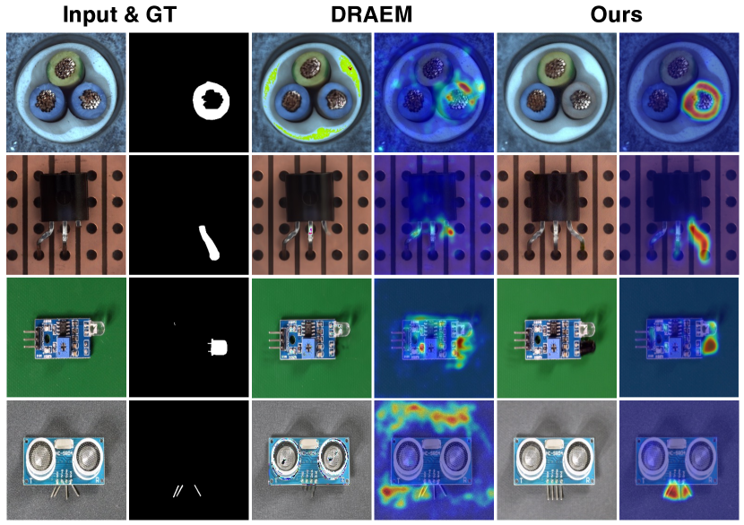
Figure 1: Anomaly detection and localization examples (Rows 1 to 4) on MVTec [4] and VisA [60]. Compared to the previous autoencoder-based approach DRAEM [58], i.e., Col. 3 & 5, our proposed DiffusionAD exhibits superior reconstruction quality consisting of anomaly-free recovery of anomalous regions and fine-grained reconstruction of normal regions. Moreover, DiffusionAD locates the various anomaly regions more accurately (Col. 4 & 6).

Given its importance, a great number of work has been devoted to anomaly detection (AD). Due to the limited number of anomaly samples and the labor-intensive labeling process, detailed anomaly samples are not available for training. As a result, most recent studies on anomaly detection have been performed without prior information about the anomaly, i.e., unsupervised paradigm [9, 37, 13]. These methods include, but are not limited to, feature embeddings and generative models. Feature embedding-based methods  [37, 13, 9, 31, 49] often suffer from degraded performance when the distribution of industrial images differs significantly from the one used for feature extraction, as they rely on pre-trained feature extractors on extra datasets such as ImageNet. Generative model-based methods  [1, 11, 58, 34, 29] require no extra data and are widely applicable in various scenarios. These approaches generally use autoencoder-based networks (AEs), based on the assumption that after the encoder has compressed the input image into a low-dimensional representation, the decoder will reconstruct the anomalous region as normal [3, 58, 16]. However, as shown in Fig. 1, the AE-based paradigm has limitations: i@) it may result in an invariant reconstruction of abnormal regions as the low-dimensional representation compressed from the original image still contains anomalous information, leading to false negative detection. ii@) AEs may perform a coarse reconstruction of normal regions due to limited restoration capability and introduce many false positives, especially on datasets with complex structures or textures.

To address the aforementioned issues, we propose a novel generative model-based framework consisting of a reconstruction sub-network and a segmentation sub-network for anomaly detection named DiffusionAD. Firstly, we reframe the reconstruction process as a noise-to-norm paradigm by introducing Gaussian noise to perturb the input image, followed by a denoising model to predict the added noise. We implement noise addition and denoising via the diffusion model [20] due to its excellent density estimation capability and high sampling quality. The proposed paradigm offers two advantages, as shown in the fifth column of Fig. 1: i@) The anomalous regions are treated as noise after losing their distinguishable features, which enables a anomaly-free reconstruction of the anomalous regions instead of an invariant one. ii@) It aims to cover the whole distribution of normal appearance [14, 20], which enables fine-grained reconstruction instead of a coarse reconstruction. After that, the segmentation sub-network predicts the pixel-wise anomaly score by exploiting the inconsistencies and commonalities between the input image and its reconstruction.

Equipped with the noise-to-norm paradigm, DiffusionAD reconstructs more satisfactory results and thus improves the performance of anomaly detection. However, as a class of likelihood-based models, diffusion models [44, 20] generally require a large number of denoising iterations (typically about 50 to 1000 steps) to obtain optimal reconstructions from randomly sampled Gaussian noise, which is much slower than the real-time requirements in practical AD scenarios as shown in Fig. 2. To address this issue, we introduce a one-step denoising paradigm for anomaly detection that employs a diffusion model to predict the noise once and then directly predict the reconstruction result. This paradigm achieves hundreds of times faster inference speed than the conventional iterative denoising paradigm while maintaining comparable recovery quality.

Nonetheless, anomaly detection consistently poses a non-trivial challenge, mainly due to the inherent diversity in the representation of anomalies. These variants encompass subtle anomalies as well as more conspicuous ones, which are characterized by larger anomaly regions or semantic alterations. We observe that different types of anomalies require different noise scales for efficient recovery, especially within the one-step denoising paradigm. Specifically, when anomalies are relatively minor, a one-step prediction stemming from a smaller noise scale proves more advantageous, yielding superior pixel-level restoration quality. For more pronounced anomalies, the strategic application of a larger noise scale to perturb them followed by a one-step reconstruction results in enhanced semantic-level restoration quality. Therefore, we further introduce a norm-guided paradigm that leverages direct predictions from larger noise scales to guide the reconstruction of smaller noise scales, leading to superior reconstruction outcomes. Ultimately, DiffusionAD achieves SOTA anomaly detection performance and fast inference speed compared to other diffusion-free paradigms, as demonstrated in Fig. 2. This truly fulfills the effectiveness and efficiency requirements of real-world application scenarios.

The main contributions of this paper are summarized in the following:

• We propose DiffusionAD, a novel pipeline that reconstructs the input image to an anomaly-free restoration via the noise-to-norm paradigm and further predicts pixel-wise anomaly scores by exploiting inconsistencies and commonalities between them.

• We propose a one-step denoising paradigm to significantly speed up the denoising process. Moreover, we propose the norm-guided paradigm to achieve superior reconstruction results.

• We conduct comprehensive experiments on four datasets to demonstrate that DiffusionAD significantly outperforms the previous SOTA by a large margin in terms of anomaly detection and localization.

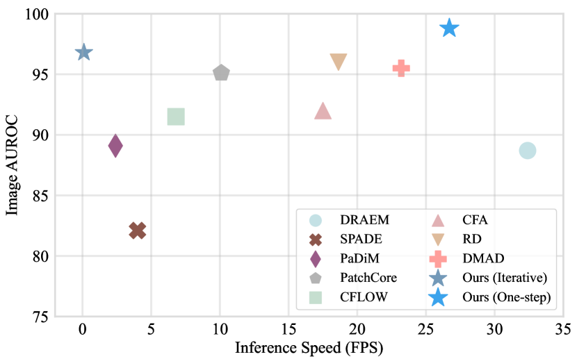
Figure 2: Comparison of different algorithms on image AUROC and inference speed. The Y-axis indicates the anomaly detection capability. The X-axis refers to the inference speed. These results are verified on the VisA [60] dataset.

2 Related Work

Anomaly Detection. Modern methods for anomaly detection encompass two main paradigms: feature embedding-based approaches [37, 13, 9, 10, 25, 26, 59, 31, 49] and generative model-based approaches [18, 57, 39, 58, 34].

Methods based on feature embeddings typically extract features of normal samples through a model pre-trained on ImageNet and then perform anomaly estimation. Built on top of extracted features, knowledge distillation [5, 40, 13, 49] estimate anomalies by comparing the differences in anomaly region features between teacher and student networks. There are also extensive studies  [9, 10, 31, 25] estimating anomalies by measuring the distance between an anomalous sample and the feature space of normal samples.

On the other hand, generative model-based methods do not require additional data. The core idea of generative model-based approaches is to implicitly or explicitly learn the feature distribution of the anomaly-free training data. Generative models based on VAE [12, 28] introduce a multidimensional normal distribution in the latent space for normal samples and then estimate the anomaly by the negative log-likelihood of the established distribution. GAN-based generative models [42, 1, 56, 16, 21] estimate anomalies through a discriminative network that compares the query image with randomly sampled samples from the latent space of the generative network. Besides, several works introduce proxy tasks based on the generative paradigm, such as image inpainting [58, 45] and attribute prediction [34, 55, 50]. Normalizing Flow-based methods [38, 18, 39, 57] combine deep feature embeddings and generative models. These methods estimate accurate data likelihoods in the latent space by learning bijective transformations between normal sample distributions and specified densities.

Diffusion Model. Diffusion models [20, 44, 47], a class of generative models inspired by non-equilibrium thermodynamics [43], define a paradigm in which the forward process slowly adds random noise to the data, and the reverse constructs the desired data samples from the noise. Recently, a wide range of diffusion-based perception applications has emerged, such as image generation [14, 20, 47, 35], image segmentation [23, 2, 17, 6], object detection [7], etc. AnoDDPM [53] tentatively explores the application of diffusion models to reconstruct medical lesions in the brain. However, it measures unhealthy outliers by squared error, leading to a high false positive rate. In addition, the iterative denoising approach employed in AnoDDPM leads to a notably slow inference speed and substantial computational cost.

3 Preliminaries

Denoising diffusion models. A family of generative models called denoising diffusion models [20, 44, 35, 43] are inspired by equilibrium thermodynamics [47, 46]. In particular, a diffusion probabilistic model specifies a forward diffusion phase in which the input data are progressively perturbed by adding Gaussian noise over several steps and then learns to reverse the diffusion process to recover the desired noise-free data from the noisy data. The forward noise process is defined as:

$$x_{t}=x_{0}\sqrt{\bar{\alpha}_{t}}+\epsilon_{t}\sqrt{1-\bar{\alpha}_{t}},\quad\epsilon_{t}\sim\mathcal{N}(\mathbf{0},\mathbf{I}),$$ (1)

which transforms a data sample $x_{0}$ into a noisy sample $x_{t}$. Here, $t$ is randomly sampled from $\{0,1,...,T\}$, $\bar{\alpha}_{t}=\prod_{i=0}^{t}\alpha_{i}=\prod_{i=0}^{t}(1-\beta_{i})$ and $\beta_{i}\in(0,1)$ represents the noise variance schedule. This can be defined as a small linear schedule [43] from $\beta_{1}=10^{-4}$ to $\beta_{T}=10^{-2}$. During training, a U-Net [36]-like architectures $\epsilon_{\theta}\left(x_{t},t\right)$ is trained to predict $\epsilon$ by minimizing the training objective:

$$\mathcal{L}=\mathbb{E}_{t\sim[1-T],x_{0}\sim q\left(x_{0}\right),\epsilon\sim\mathcal{N}(0,\mathbf{I})}\left[\left\|\epsilon-\epsilon_{\theta}\left(x_{t},t\right)\right\|^{2}\right].$$ (2)

At inference stage, $x_{t-1}$ is reconstructed from noise $x_{t}$ with the model $\epsilon_{\theta}\left(x_{t},t\right)$ according to:

$$x_{t-1}=\frac{1}{\sqrt{\alpha_{t}}}\left(x_{t}-\frac{1-\alpha_{t}}{\sqrt{1-\bar{\alpha}_{t}}}\epsilon_{\theta}\left(x_{t},t\right)\right)+\tilde{\beta}_{t}z.$$ (3)

where $z\sim\mathcal{N}(\mathbf{0},\mathbf{I})$ and $\tilde{\beta}_{t}=\frac{1-\bar{\alpha}_{t-1}}{1-\bar{\alpha}_{t}}\beta_{t}$. $x_{0}$ is reconstructed from $x_{t}$ in an iterative way, i.e., $x_{t}\rightarrow x_{t-1}\rightarrow\ldots\rightarrow x_{0}$.

Classifier guidance and image guidance. To improve the quality and diversity of generated samples, guided diffusion [14] uses a pre-trained classifier $p_{\phi}(y|x_{t})$ to guide the diffusion sampling process, where $y$ is the class label. The guiding process is defined as modifying the noise prediction by a guidance scale $w$:

$$\epsilon_{\theta}(x_{t},t,y)=\epsilon_{\theta}(x_{t},t)-\sqrt{1-\bar{\alpha}_{t}}\mathrm{~{}}w\nabla_{x_{t}}\log p_{\phi}(y|x_{t})$$ (4)

Thus, the impact of class $y$ on the generated results can be controlled by adjusting the parameter $w$.

To achieve a more diverse form of control, SDG [30] utilizes the reference image $r$ to guide the sampling process and reformulates Eq. 4 as follows:

$$\epsilon_{\theta}({x_{t},t,r_{t})=\epsilon_{\theta}(x_{t},t)-\sqrt{1-\bar{\alpha}_{t}}\mathrm{~{}}w\nabla_{x_{t}}sim(x_{t},r_{t})}$$ (5)

where $r_{t}$ is obtained from Eq. 1 by perturbing $r$ and $sim(\cdot,\cdot)$ is a measure of the similarity or correlation between two images.

4 Methodology

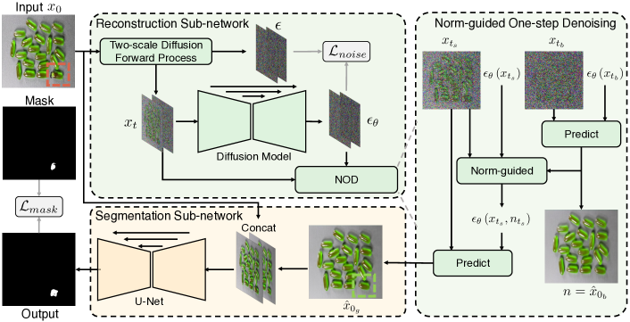
Figure 3: An overview of the proposed pipeline DiffusionAD. The reconstruction and segmentation sub-networks constitute the entire pipeline. The input image is perturbed by two distinct noise scales. Following, the noise is predicted by an inference within the diffusion model. Finally, the norm-guided one-step denoising paradigm is employed to predict an anomaly-free reconstruction. The segmentation sub-network predicts pixel-wise anomaly scores by comparing commonalities and inconsistencies between the input image and its reconstruction.

4.1 Architecture

Our proposed novel generative model-based framework consists of two components: a reconstruction sub-network and a segmentation sub-network, as shown in Fig. 3. With the proposed anomaly generation strategies (Sec. 4.4), We define $x_{0}$ as the input image that is either normal ($y=0$) or anomalous ($y=1$).

Reconstruction sub-network. We implement the reconstruction sub-network via a diffusion model, which reformulates the reconstruction process as a noise-to-norm paradigm. First, we use the diffusion forward process proposed [20] to corrupt the input image $x_{0}$ at a random time step $t$ to obtain $x_{t}$ via Eq. 1. The input image $x_{0}$ gradually loses its discriminative features and approaches an isotropic Gaussian distribution as the time step increases. Then $\epsilon_{\theta}\left(x_{t},t\right)$ is a function approximator intended to predict noise $\epsilon$ from ${x}_{t}$ and $t$, which is implemented with a U-Net [36, 14]-like architecture based on PixelCNN [41], ResNet [19], and Transformer [51]. It is worth noting that after being perturbed by Gaussian noise, the anomalous pixels lose their distinctive features and tend to be treated by the model as injected noise. Consequently, the anomaly-free reconstruction $\hat{x}_{0}$ can be obtained from Eq. 3 in an iterative manner.

Segmentation sub-network. The segmentation sub-network employs a U-Net [36]-like architecture consisting of an encoder, a decoder, and skip connections. The input to the segmentation sub-network is a channel-wise concatenation of $x_{0}$ and $\hat{x}_{0}$. The segmentation sub-network learns to identify anomalies by exploiting the inconsistencies and commonalities between the input image $x_{0}$ and its anomaly-free approximation $\hat{x}_{0}$ to predict the pixel-wise anomaly score without post-processing. Remarkably, the learned inconsistency reduces false positives caused by slight pixel-wise differences between the normal region and its reconstruction and highlights significantly different regions.

4.2 Norm-guided One-step Denoising

Each iteration of the denoising process in the diffusion model corresponds to a round of network inference, requiring substantial computational resources and time. This presents a significant challenge for real-time inference.

One-step Denoising. To this end, we employ a direct reconstruction method, which we refer to as one-step denoising, as an alternative to the iterative approach. More specifically, at any time step $t$, after the diffusion model predicts the noise $\epsilon_{\theta}\left(x_{t},t\right)$ of $x_{t}$ by a single inference (one-step), direct recovery is always valid [20], as indicated by the following:

$$\hat{x}_{0}=\frac{1}{\sqrt{\bar{\alpha}_{t}}}\left(x_{t}-\sqrt{1-\bar{\alpha}_{t}}\epsilon_{\theta}\left(x_{t},t\right)\right).$$ (6)

where $\hat{x}_{0}$ refers to the anomaly-free reconstruction via one-step denoising. This direct prediction is $t$ times faster than iterative prediction, resulting in significant savings of computational resources and inference time. However, we observe that repairing different types of anomalies requires different scales of noise injection. When the anomaly region is relatively small or absent, direct prediction from $x_{t_{s}}$ is more suitable, as shown in Fig. 4 (b). The anomaly-free restoration $\hat{x}_{0_{s}}$ demonstrates higher pixel quality, preserving fine-grained details and closely aligning with the iterative result. Conversely, predicting directly from $x_{t_{b}}$ introduces some distortions, and as the time step $t$ increases, these distortions gradually amplify. In cases where the anomaly region is larger or exhibits semantic changes, predicting from $x_{t_{s}}$ leaves some residual anomaly regions, as illustrated in Fig. 4 (b). Therefore, the injection of noise at larger scales becomes necessary to effectively perturb the anomalous regions in order to achieve higher quality, anomaly-free restoration $\hat{x}_{0_{b}}$ at the semantic level.

Norm-guided Denoising. In order to harness the advantages of both noise scale regimes, we propose a norm-guided denoising paradigm. We divide the random range of $t\in\{0,1,...,T\}$ into two parts using $\tau$, where $S=\{0,1,...,\tau\}$ and $B=\{\tau+1,\tau+2,...,T\}$. For an input image $x_{0}$, we first perturb it using two randomly sampled time steps $t_{s}\in S$ and $t_{b}\in B$ to obtain $x_{t_{s}}$ and $x_{t_{b}}$ through Eq. 1. As the diffusion model defaults to being conditioned on $t$, we abbreviate $\epsilon_{\theta}(x_{t},t)$ as $\epsilon_{\theta}(x_{t})$. Subsequently, we first employ the diffusion model to individually predict the noise of $x_{t_{s}}$ and $x_{t_{b}}$, corresponding to $\epsilon_{\theta}(x_{t_{s}})$ and $\epsilon_{\theta}(x_{t_{b}})$, respectively. We then directly predict $\hat{x}_{0_{b}}$ using $\epsilon_{\theta}(x_{t_{b}})$ by Eq. 6. Although $\hat{x}_{0_{b}}$ exhibits some distortions and appears low in mass, it consistently presents an anomaly-free appearance despite the diversity of anomalies in $x_{0}$. Hence, $\hat{x}_{0_{b}}$ is regarded as $\hat{x}_{0_{b}}\sim q(x_{y=0})$ and is rewritten as $n$. After that, $n$ assumes the role of a conditional image to guide the prediction of $\hat{x}_{0_{s}}$ by Eq. 5. We define $sim(x_{t},n_{t})=-\frac{1}{2}~{}(n_{t_{s}}-x_{t_{s}})^{2}$ to measure the similarity between these two images. $n_{t_{s}}$ is obtained by perturbing $n$ with the predicted noise $\epsilon_{\theta}(x_{t_{s}})$ instead of random noise in order to make the guidance more dependent on the difference between the image contents themselves. Thus, Eq. 5 is reformulated as follows:

$$\epsilon_{\theta}(x_{t_{s}},n_{t_{s}})=\epsilon_{\theta}(x_{t_{s}})-\sqrt{1-\bar{\alpha}_{t_{s}}}\mathrm{~{}}w\mathrm{~{}}(n_{t_{s}}-x_{t_{s}})$$ (7)

where $\epsilon_{\theta}(x_{t_{s}},n_{t_{s}})$ denotes the modified noise with norm-guidance. Finally, bring $x_{t_{s}}$ and $\epsilon_{\theta}(x_{t_{s}},n_{t_{s}})$ into Eq. 6 to directly predict the norm-guided anomaly-free reconstruction as follows:

$$\hat{x}_{0_{g}}=\frac{1}{\sqrt{\bar{\alpha}_{t_{s}}}}\left(x_{t_{s}}-\sqrt{1-\bar{\alpha}_{t_{s}}}\epsilon_{\theta}\left(x_{t_{s}},n_{t_{s}}\right)\right).$$ (8)

Equipped with the norm-guided denoising paradigm, DiffusionAD can handle different types of anomalies and predict superior reconstructions.

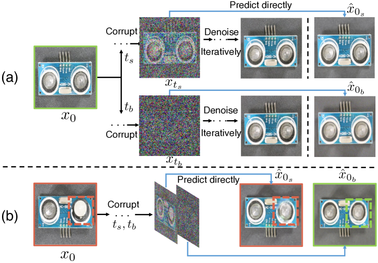
Figure 4: Two-scale corruptions and their different reconstructions.

4.3 Training & Inference

Training stage.  We jointly train the denoising and segmentation sub-networks. The diffusion model learns the entire distribution of normal samples ($y=0$) by minimizing the following loss function:

$$\mathcal{L}_{noise}=\frac{(1-y)(\|\epsilon_{t_{s}}-\epsilon_{\theta}(x_{t_{s}})\|^{2}+\|\epsilon_{t_{b}}-\epsilon_{\theta}(x_{t_{b}})\|^{2})}{2}.$$ (9)

The segmentation sub-network exploits the commonalities and differences between $x_{0}$ and $\hat{x}_{0_{g}}$ to predict pixel-wise anomaly scores as close as possible to the ground truth mask. The segmentation loss is defined as:

$$\mathcal{L}_{mask}=\operatorname{Smooth}_{\mathcal{L}1}\left(M,\hat{M}\right)+\gamma\mathcal{L}_{focal}\left(M,\hat{M}\right).$$ (10)

Where $M$ is the ground truth mask of the input image and $\hat{M}$ is the output of the segmentation sub-network. Inspired by  [59], smooth L1 loss [15] and focal loss [27] are applied simultaneously to reduce over-sensitivity to outliers and accurately segment hard anomalous examples. $\gamma\in\mathbb{R}^{+}$ is a hyperparameter that controls the importance of $\mathcal{L}_{focal}$. Thus, the total loss used in jointly training DiffusionAD is:

$$\mathcal{L}_{total}=\mathcal{L}_{noise}+\mathcal{L}_{mask}.$$ (11)

Inference stage. Unlike other diffusion methods that reconstruct images in an iterative manner, we still perform a one-step norm-guided estimation in the inference stage, which is hundreds of times faster while maintaining comparable sampling quality. The robust decision boundary learned by the segmentation network will also effectively mitigate the effect of such sub-optimal sample quality. Moreover, in the inference phase, $t_{s}$ and $t_{b}$ are fixed values. After the segmentation model predicts the pixel-level anomaly score $\hat{M}$, we take the average of the top $K$ anomalous pixels in $\hat{M}$ as the image-level anomaly score [59].

4.4 Anomaly Synthetic Strategy

Since prior information about anomalies is not available for training, we synthesize pseudo-anomalies online for end-to-end training. The idea of our anomaly synthesis strategy is adding visually inconsistent appearances to the normal samples inspired by  [59, 58, 54], and these out-of-distribution regions are defined as the synthesized anomalous regions.

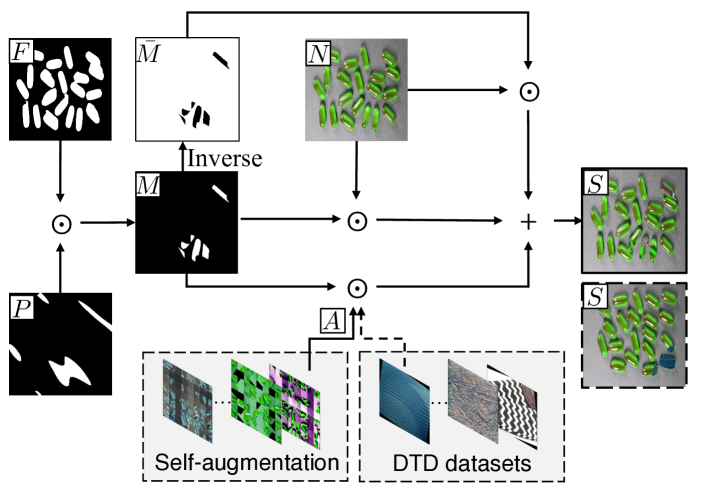
Figure 5: Visually inconsistent appearances are added to the normal samples to obtain synthetic anomalies.

Fig. 5 illustrates the overall process of transforming a normal sample (Fig. 5, $N$) into a synthetic anomalous sample (Fig. 5, $S$). Random and irregular anomalous regions (Fig. 5, $P$) are first obtained from the Perlin [32] noise and then multiplied by the object foreground [33] (Fig. 5, $F$) of the normal sample to obtain the ground truth mask (Fig. 5, $M$). For textural datasets, the foreground is replaced by a random part of the whole image. The appearance of visual inconsistencies (Fig. 5, $A$) mainly stems from the self-augmentation of normal samples or Describing Textures Dataset (DTD) [8]. The proposed synthetic anomaly (Fig. 5, $S$) is defined as:

$$S=\beta(M\odot N)+(1-\beta)(M\odot A)+\bar{M}\odot N$$ (12)

where $\bar{M}$ is the pixel-wise inverse operation of $M$, $\odot$ is the element-wise multiplication operation, and $\beta$ serves as an opacity parameter designed to enhance the fusion of anomalous and normal regions.

5 Experiments

5.1 Experimental Details

Datasets. To assess the efficacy and generalizability of our approach, we conduct experiments on four diverse unsupervised datasets including MVTec [4], VisA [60], DAGM [52], and MPDD [22]. These datasets contain samples of many different types of surface defects, such as scratches, cracks, holes, and depressions.

Evaluation Metrics. To measure the performance of anomaly detection (image level), we report the Area Under Receiver Operator Characteristic curve (Image AUROC), the most widely used metric. In terms of anomaly localization (pixel level) performance, we report three metrics: Pixel AUROC, PRO, and Pixel AP. Pixel AUROC may provide an inflated view of the performance [60], which may pose challenges in measuring the true capabilities of the model when using only this metric. The false positive rate is dominated by the extremely high number of non-anomalous pixels and remains low despite the false positive prediction [48], which is caused by the fact that anomalous regions typically only occupy a tiny fraction of the entire image. Thus, to comprehensively evaluate the anomaly localization performance, Per Region Overlap (PRO) and pixel-level Average Precision (AP) also play the role of evaluation metrics. Per Region Overlap (PRO) metric is more capable of assessing the ability of fine-grained anomaly localization, which treats anomaly regions of varying sizes equally and is widely employed by previous works [13, 37, 59]. AP is more appropriate for highly imbalanced classes, especially for industrial anomaly localization, where accuracy is critical.

Implementation Details. All images in the four datasets are resized to $256\times 256$. For the denoising sub-network, we adopt the UNet [36] architecture for estimating $\epsilon_{\theta}$. This architecture is mainly based on PixelCNN [41] and Wide ResNet [19], with sinusoidal positional embedding [51] to encode the time step $t$. $T$ is set to 1000 and is divided by $\tau=300$ into two parts. The noise schedule is set to linear. We set the base channel to 128, the attention resolutions to 32, 16, 8, and the number of heads to 4. We do not use EMA. For the segmentation sub-network, we employ a U-Net-like architecture consisting of an encoder, a decoder, and skip connections. $\gamma$ in the segmentation loss $\mathcal{L}_{seg}$ is set to 5. We train for 3000 epochs with a batch size of 16 consisting of 8 normal samples and 8 anomalous synthetic samples. We use Adam optimizer [24] for optimization, with an initial learning rate $10^{-4}$. The image-level anomaly score is obtained by taking the average of the top 50 anomalous pixels in pixel-wise anomaly score $\hat{M}$. We implement our model and experiments on NVIDIA A100 GPUs.

	Feature embedding-based				Generative model-based
Category	PatchCore [37]	RD4AD [13]	RD++ [49]	SimpleNet [31]	DMAD [29]	DRAEM [58]	FastFlow [57]	Ours
candle	98.6/94.0	92.2/92.2	96.4/93.8	98.7/89.0	92.7/90.6	94.4/93.7	92.8/86.7	98.7/97.0
capsules	81.6/85.5	90.1/56.9	92.1/95.8	89.9/91.4	88.0/88.4	76.3/84.5	71.2/33.3	97.9/98.7
cashew	97.3/94.5	99.6/79.0	97.8/91.2	97.5/82.8	95.0/88.8	90.7/51.8	91.0/68.3	96.5/91.8
chewinggum	99.1/84.6	99.7/92.5	96.4/88.1	99.8/85.3	97.4/73.9	94.2/60.4	91.4/74.8	99.9/92.2
fryum	96.2/85.3	96.6/81.0	95.8/90.0	98.1/87.8	98.0/92.2	97.4/93.1	88.6/74.3	98.3/96.5
macaroni1	97.5/95.4	98.4/71.3	94.0/96.9	99.4/98.9	94.3/97.1	95.0/96.7	98.3/77.7	99.5/98.5
macaroni2	78.1/94.4	97.6/68.0	88.0/97.7	82.4/97.3	90.4/98.5	96.2/99.6	86.3/43.4	99.0/99.6
pcb1	98.5/94.3	97.6/43.2	97.0/95.8	99.0/91.1	95.8/96.2	54.8/24.8	77.4/59.9	99.2/96.9
pcb2	97.3/89.2	91.1/46.4	97.2/90.6	99.1/91.0	96.9/89.3	77.8/49.4	61.9/40.7	99.1/94.2
pcb3	97.9/90.9	95.5/80.3	96.8/93.1	98.5/93.0	98.3/93.6	94.5/89.7	74.3/61.5	98.6/94.9
pcb4	99.6/90.1	96.5/72.2	99.8/91.9	99.6/64.5	99.7/91.4	93.4/64.3	80.9/58.8	98.9/94.6
pipe_fryum	99.8/95.7	97.0/68.3	99.6/95.6	99.7/91.7	99.0/95.3	99.4/75.9	72.0/38.0	99.8/97.2
Average	95.1/91.2	96.0/70.9	95.9/93.4	96.8/88.7	95.5/91.3	88.7/73.7	82.2/59.8	98.8/96.0

Table 1: Anomaly Detection and Localization on VisA [60]. The best results of Image AUROC / Pixel PRO are highlighted in bold.

5.2 Anomaly Detection and Localization Results

We compare the anomaly detection and localization performance of DiffusionAD with four feature embedding-based methods, i.e., PatchCore [37], RD4AD [13], RD++ [49], SimpleNet [31] and three generative model-based methods, i.e., DMAD [29], FastFlow [57] and DRAEM [58].

Per-class performance on VisA. The results of anomaly detection (Image AUROC) and anomaly localization (PRO) on the VisA dataset are shown in Tab. 1. Our method achieves the highest image AUROC and the highest PRO in 10 out of 12 classes. The average image AUROC results show that our method outperforms feature embedding-based SOTA by 2.0% and generative model-based SOTA by 3.3%. Meanwhile, for PRO, our method outperforms feature embedding-based SOTA by 2.6% and generative model-based SOTA by 4.7%. In some hard cases, such as capsules and macaroni2, DiffusionAD outperforms previous generative model-based methods by a large margin.

	VisA [60]				MVTec [4]				DAGM [52]				MPDD [22]				Average
	I $\uparrow$	P $\uparrow$	O $\uparrow$	A $\uparrow$	I $\uparrow$	P $\uparrow$	O $\uparrow$	A $\uparrow$	I $\uparrow$	P $\uparrow$	O $\uparrow$	A $\uparrow$	I $\uparrow$	P $\uparrow$	O $\uparrow$	A $\uparrow$	I $\uparrow$	P $\uparrow$	O $\uparrow$	A $\uparrow$
PatchCore	95.1	98.8	91.2	40.1	99.1	98.1	93.5	56.1	93.6	96.7	89.3	51.7	94.8	99.0	93.9	43.2	95.7	98.2	92.0	47.8
RD4AD	96.0	90.1	70.9	27.7	98.5	97.8	93.9	58.0	95.8	97.5	93.0	53.4	92.7	98.7	95.3	45.5	95.8	96.0	88.3	46.2
RD++	95.9	98.7	93.4	40.8	99.4	98.3	95.0	60.8	98.5	97.4	93.8	64.3	92.9	98.3	94.9	43.7	96.7	98.2	94.3	52.4
SimpleNet	96.8	97.8	88.7	36.3	99.6	97.6	90.0	54.8	95.3	97.1	91.3	48.1	96.1	97.6	91.2	40.7	96.9	97.5	90.3	45.0
DMAD	95.5	98.6	91.3	41.0	99.6	98.2	90.6	53.5	89.1	92.5	83.8	46.0	91.7	98.0	92.6	42.6	94.0	96.8	89.6	45.8
FastFlow	82.2	88.2	59.8	15.6	90.5	95.5	85.6	39.8	87.4	91.1	79.9	34.2	88.7	80.8	49.8	11.5	87.2	88.9	68.8	25.3
DRAEM	88.7	94.4	73.7	30.5	98.0	97.3	92.1	68.4	90.8	86.8	71.0	30.6	94.1	91.8	78.1	28.8	92.9	92.6	78.7	39.6
Ours	98.8	98.9	96.0	45.8	99.7	98.7	95.7	76.1	99.6	97.5	93.8	65.1	96.2	98.5	95.3	45.8	98.6	98.4	95.2	58.2

Table 2: Comparison of DiffusionAD with other approaches on four datasets. “I”, “P”, “O” and “A” respectively refer to the four metrics of image auroc, pixel auroc, pixel pro and pixel ap. Best results are highlighted in bold.

Quantitative results across the four datasets. Tab. 2 enumerates the performance of the aforementioned methods across the four datasets. We conduct a comprehensive comparison based on four metrics, which include image AUROC for anomaly detection and pixel AUROC, PRO, and pixel AP for anomaly localization. In addition to its performance on the VisA dataset, DiffusionAD achieves state-of-the-art results on another widely used dataset, MVTec, across four key metrics. Remarkably, DiffusionAD outperforms the previous feature embedding-based SOTA by 15.3% and the previous generative model-based SOTA by 7.7% in terms of average pixel AP metric. Our method also outperforms previous approaches on the DAGM and MPDD datasets, especially in terms of average image AUROC. Finally, we evaluate the generalization ability of the method by measuring its average performance across the four datasets. As shown in Tab. 2, our approach significantly outperforms previous methods and in particular, outperforms previous generative models by a large margin. More details will be provided in Sec. 7.

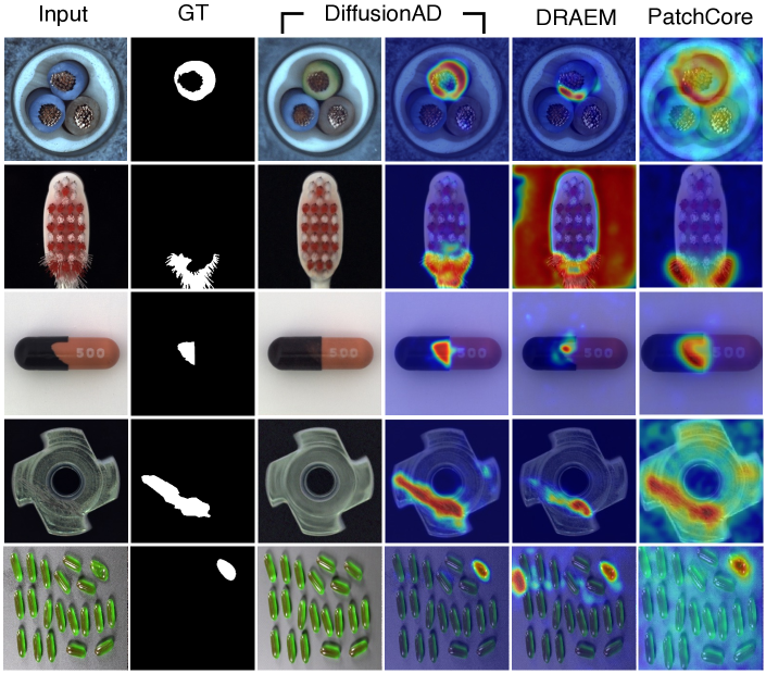
Figure 6: Qualitative results on MVTec [4] and VisA [60].

Qualitatively evaluate on anomaly localization. According to the results in Fig. 6, we qualitatively assess the performance of DiffusionAD on anomaly detection and localization compared to the previous feature embedding-based method PatchCore [37] and generative model-based method DRAEM [58]. These images are sub-datasets of MVTec [4] and Visa [60], where the anomalous regions vary in shape, size and number, as shown in the first and second columns of Fig. 6. The third and fourth columns show the reconstruction and anomaly localization results of DiffusionAD, respectively. It can be observed that the reconstruction sub-network successfully repairs various types of anomalies while maintaining high image fidelity. After that, the segmentation sub-network accurately predicts the pixel-wise anomaly score using the input image and its anomaly-free reconstruction, leading to more accurate anomaly localization than previous methods such as DRAEM [58] and PatchCore [37].

5.3 Ablation Study

The importance of architecture and denoising paradigm. Tab. 3 illustrates the impact of different architectures and denoising methods on performance and inference speed. We introduce FPS (Frames Per Second) to evaluate the inference speed. As indicated in the first row of Tab. 3, the performance of anomaly detection and localization is limited due to the unsatisfactory reconstruction results of the Autoencoder (AE.). However, its inference speed is notably fast. When we adopt the proposed noise-to-norm paradigm, as seen in the second row, which utilizes higher-quality reconstructions from the diffusion model (DM.), the performance is significantly enhanced. Nonetheless, each denoising iteration (Ite.) corresponds to one network inference (in this case, 400 iterations in total), which falls significantly short of the real-world requirements for inference speed. In the third row, when we employ the proposed one-step (OS.) denoising, the inference speed is approximately 300 times faster than the iterative approach. Simultaneously, there is an improvement in both anomaly detection and localization performance. We attribute this to the comparable quality of one-step reconstruction results and the consistent training and inference paradigm, where the segmentation sub-network always receives the one-step reconstructions during training. In the fourth row, the norm-guided (NG.) paradigm combines the advantages of both one-step reconstructions from different noise scales, leading to further performance enhancements while maintaining comparable inference speed.

Architecture			Denoising			Performance
Seg.	AE.	DM.	Ite.	OS.	NG.	I $\uparrow$	P $\uparrow$	O $\uparrow$	A $\uparrow$	F $\uparrow$
$\checkmark$	$\checkmark$					90.6	96.2	76.1	31.9	32.4
$\checkmark$		$\checkmark$	$\checkmark$			96.8	98.5	92.5	42.5	0.09
$\checkmark$		$\checkmark$		$\checkmark$		98.0	98.6	94.7	44.2	26.7
$\checkmark$		$\checkmark$		$\checkmark$	$\checkmark$	98.8	98.9	96.0	45.8	23.5

Table 3: Impact of modules and denoising paradigms.

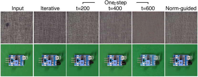
Figure 7: Impact of noise scale on anomaly-free reconstruction.

The effect of noise scale. We investigate how the added noise scale of the input individually affects the reconstruction results and anomaly detection performance. First, Fig. 7 illustrates the effect of the noise scale on the quality of the reconstruction. The second column of Fig. 7 shows the gradual denoising results from $t=400$, which can be considered as the ideal recovery. For one-step reconstruction, direct prediction becomes more challenging as the noise scale increases, resulting in lower pixel quality. However, repairing more pronounced anomalies often requires larger noise scales to perturb the anomalies, leading to reconstructions with higher semantic quality. Thus, the norm-guided one-step approach combines the advantages of both scales, resulting in a reconstruction that encompasses both pixel and semantic quality, closely approximating the quality of the iterative one.

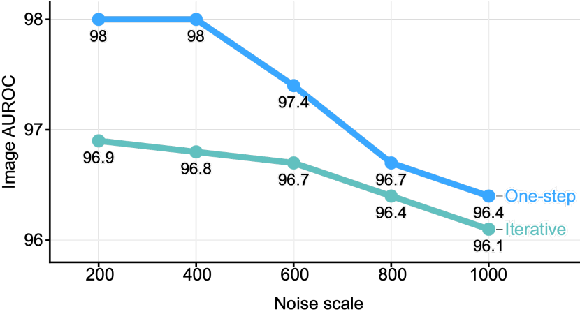
Figure 8: Impact of noise scale on anomaly detection performance.

Fig. 8 further depicts the effect of different noise scales on the anomaly detection performance. In the iterative approach, the predictions of the segmentation network show little variation, as the reconstruction results are consistent. However, the inference time increases with $t$. In the one-step denoising approach, the inference time remains constant, but there is a decrease in Image AUROC as $t$ becomes relatively large, mainly due to the reduced reconstruction quality. It is worth noting that the proposed one-step denoising paradigm consistently achieves superior anomaly detection performance compared to the iterative one.

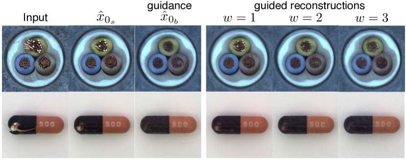
Figure 9: Ablations of guidance scale.

Effects of guidance scale. As shown in Fig. 9, the influence of conditional information becomes more significant as the guidance scale $w$ increases. In this paper, $w$ is set to 1 as an empirical choice.

6 Conclusion

In this paper, we present DiffusionAD, a novel anomaly detection pipeline consisting of a reconstruction sub-network and a segmentation sub-network. Firstly, we redefine the reconstruction process using a diffusion model, adopting the noise-to-norm paradigm where anomalous regions are perturbed by Gaussian noise and then reconstructed to appear normal. Secondly, we present a one-step denoising paradigm, which is significantly faster than the iterative denoising approach in diffusion models. In addition, we propose the norm-guided paradigm to further enhance the reconstruction quality. Finally, the segmentation sub-network exploits the inconsistencies and commonalities between the input image and its anomaly-free restoration to predict pixel-level anomaly scores. Extensive evaluations across four datasets demonstrate that DiffusionAD outperforms current state-of-the-art methods, highlighting the effectiveness and wide applicability of this novel pipeline.

7 Appendix

Datasets. (1) The MVTec [4] dataset is widely used to evaluate and test anomaly detection algorithms and industrial defect detection, consisting of 4,096 normal and 1,258 abnormal images. It contains samples of many different types of surface defects, such as scratches, cracks, holes, and depressions. (2) VisA [60] is a novel and challenging dataset consisting of 10,821 images (9,621 normal and 1,200 abnormal images) in total, which is $2\times$ larger than MVTec. Visa contains 12 subsets, which can be divided into three broad categories based on the properties of the objects. The first category consists of four printed circuit boards (PCBS) with complex structures. The second type is a dataset with multiple instances in one view and consists of Capsules, Candles, Macaroni1, and Marcaroni2. The third type is single instances with roughly aligned objects: Cashew, Chewing gum, Fryum, and Pipe fryum. Anomalous images in VisA contain a variety of imperfections, including surface defects such as scratches, dents, colored spots, or cracks, and structural defects such as misplacement or missing parts. (3) DAGM [52] consists of ten texture classes with 15,000 normal images and 2,100 abnormal images. Various defects that are visually close to the background, such as scratches and specks, constitute anomalous samples. (4) MPDD [22] contains 1064 normal images and 282 abnormal images. It focuses on metal fabrication and reflects real-world situations encountered on manually operated production lines.

More quantitative results on four datasets.  We extensively evaluate the performance of DiffusionAD on subclasses of four datasets, comparing it with previous state-of-the-art (SOTA) methods based on feature embedding and generative models. Tab. 4 presents a comparison of anomaly localization performance on the VisA [60] dataset, including both pixel pro and pixel ap metrics. DiffusionAD outperforms the previous generative model-based SOTA by 4.8% on average pixel AP. Tab. 5 and Tab. 6 show the comparison of anomaly detection and localization performance on the MVTec [4] dataset, indicating that DiffusionAD significantly surpasses previous generative model-based SOTA in anomaly localization, especially with improvements of 3.6% and 7.7% on pixel PRO and AP, respectively. Tab. 7 provides a detailed description of the comparison on the DAGM [52] dataset, where it outperforms previous methods in 9 out of 10 categories, achieving the highest overall image AUROC of 99.6%. This performance approaches full-recall anomaly detection. In Tab. 8, DiffusionAD demonstrates outstanding anomaly detection and localization performance on the MPDD [22] dataset, surpassing previous generative model-based methods by a large margin. These experimental results thoroughly demonstrate the effectiveness and generality of the proposed pipeline.

	Feature embedding-based				Generative model-based
Category	PatchCore [37]	RD4AD [13]	RD++ [49]	SimpleNet [31]	DMAD [29]	DRAEM [58]	FastFlow [57]	Ours
candle	99.5/17.6	97.9/19.0	98.6/16.3	97.7/12.8	98.1/18.9	97.3/32.7	94.9/4.9	99.2/49.7
capsules	99.5/68.7	89.5/12.3	99.4/57.1	99.0/57.9	99.2/50.5	99.1/47.9	75.3/1.4	99.5/51.8
cashew	98.9/58.5	95.8/28.2	95.8/53.9	98.8/58.6	95.3/57.3	88.2/28.5	91.4/9.2	98.9/61.4
chewinggum	99.1/42.8	99.0/58.9	99.4/65.8	98.3/17.7	97.9/56.1	97.1/39.0	98.6/43.6	99.3/50.0
fryum	93.8/37.2	94.3/54.3	96.5/49.7	91.1/38.0	97.0/49.2	92.7/41.1	97.3/35.3	98.2/51.5
macaroni1	99.8/7.6	97.7/43.8	99.7/21.1	99.6/6.7	99.7/16.3	99.7/45.8	97.3/27.8	99.2/41.3
macaroni2	99.1/3.2	87.7/35.2	99.7/11.1	98.9/4.4	99.7/9.8	99.9/41.0	89.2/29.8	99.9/44.1
pcb1	99.9/91.7	75.0/0.5	99.7/82.6	99.6/88.6	99.8/82.8	90.5/28.1	75.2/0.2	97.8/25.6
pcb2	99.0/14.3	64.8/0.6	99.0/14.8	98.3/12.5	99.0/14.7	90.5/4.9	67.3/0.1	98.6/15.0
pcb3	99.2/38.9	95.5/59.1	99.2/20.1	99.2/44.3	99.3/29.6	98.6/20.3	94.8/23.7	99.4/50.6
pcb4	98.6/42.4	92.8/10.6	98.6/42.6	93.9/34.0	98.8/46.8	88.0/20.6	89.9/5.4	97.6/43.1
pipe_fryum	99.1/58.5	92.0/10.4	99.1/54.9	98.9/60.5	99.3/60.2	90.9/16.5	87.3/5.4	99.0/64.9
Average	98.8/40.1	90.1/27.7	98.7/40.8	97.8/36.3	98.6/41.0	94.4/30.5	88.2/15.6	98.9/45.8

Table 4: Anomaly Localization on VisA [4]. The best results of Pixel AUROC / Pixel AP are highlighted in bold.

	Feature embedding-based				Generative model-based
Category	PatchCore [37]	RD4AD [13]	RD++ [49]	SimpleNet [31]	DMAD [29]	DRAEM [58]	FastFlow [57]	Ours
Carpet	98.7/99.0	98.9/98.8	100/99.2	99.0/98.4	100/99.1	97.0/95.5	87.5/98.0	99.3/99.0
Grid	98.2/98.7	100/97.0	100/99.3	97.8/98.9	100/99.2	99.9/99.7	88.1/93.5	100/99.7
Leather	100/99.3	100/98.6	100/99.4	99.3/98.0	100/99.5	100/98.6	96.1/93.0	100/99.8
Tile	98.7/95.6	99.3/98.9	99.7/96.6	99.7/96.6	100/96.0	99.6/99.2	63.2/96.1	99.9/99.7
Wood	99.2/95.0	99.2/99.3	99.3/95.8	99.9/93.2	100/95.5	99.1/96.4	90.8/95.9	99.9/96.7
Bottle	100/98.6	100/99.0	100/98.8	100/94.0	100/98.9	99.2/99.1	100/92.7	99.7/99.1
Cable	99.5/98.4	95.0/99.4	99.2/98.4	99.9/98.7	99.1/98.1	91.8/94.7	91.2/97.5	99.6/98.1
Capsule	98.1/98.8	96.3/97.3	99.0/98.8	100/97.4	98.9/98.3	98.5/94.3	99.2/97.4	98.9/98.3
Hazelnut	100/98.7	99.9/98.2	100/99.2	100/98.6	100/99.1	100/99.7	98.8/98.9	100/99.7
Metal nut	100/98.4	100/99.6	100/98.1	100/97.0	100/97.7	98.7/99.5	90.8/98.1	100/99.7
Pill	96.6/97.4	99.6/95.7	98.4/98.3	100/98.8	97.3/98.7	98.9/97.6	98.0/92.3	99.0/99.3
Screw	98.1/99.4	97.0/99.1	98.9/99.7	100/98.0	100/99.6	93.9/97.6	97.8/99.4	99.4/99.0
Toothbrush	100/98.7	99.5/93.0	100/99.1	98.1/99.2	100/99.4	100/98.1	100/92.7	100/98.8
Transistor	100/96.3	96.7/95.4	98.5/94.3	100/97.8	98.7/95.4	93.1/90.9	88.1/94.3	99.8/92.9
Zipper	99.4/98.8	98.5/98.2	98.6/98.8	100/99.2	99.6/98.3	100/98.8	67.5/93.4	100/99.2
Average	99.1/98.1	98.5/97.8	99.4/98.3	99.6/97.6	99.6/98.2	98.0/97.3	90.5/95.5	99.7/98.7

Table 5: Anomaly Detection and Localization on MVTec [4]. The best results of Image AUROC / Pixel AUROC are highlighted in bold.

	Feature embedding-based				Generative model-based
Category	PatchCore [37]	RD4AD [13]	RD++ [49]	SimpleNet [31]	DMAD [29]	DRAEM [58]	FastFlow [57]	Ours
Carpet	96.6/76.8	97.0/78.7	97.7/63.6	93.2/79.8	86.1/44.6	92.0/53.5	84.2/68.8	95.0/77.2
Grid	95.9/65.3	97.6/52.7	97.7/48.5	92.8/42.1	72.4/7.4	97.8/65.7	83.8/27.6	98.9/68.8
Leather	98.9/44.2	99.1/45.1	99.2/50.1	87.4/43.3	97.7/41.3	96.8/75.3	91.0/41.8	98.9/69.2
Tile	87.4/62.7	90.6/57.4	92.4/53.4	87.4/28.8	82.7/54.3	97.4/92.3	81.8/20.5	98.3/97.1
Wood	89.6/32.5	90.9/49.2	93.3/52.0	86.2/59.8	86.3/44.4	92.8/77.7	85.1/53.9	90.3/77.4
Bottle	96.1/53.7	96.6/62.1	97.0/79.9	82.2/45.2	96.0/78.9	96.4/86.5	91.9/45.5	96.8/89.7
Cable	92.6/45.6	91.0/48.2	93.9/62.5	94.7/63.7	95.1/58.3	75.4/52.4	80.8/35.1	95.5/72.5
Capsule	95.5/87.0	95.8/79.1	96.4/48.1	92.0/66.6	89.7/41.4	90.4/49.4	76.7/27.6	93.3/59.2
Hazelnut	93.9/77.7	95.5/78.4	96.3/65.4	91.9/40.4	96.4/60.2	97.5/92.9	89.0/63.3	97.5/92.6
Metal nut	91.3/35.4	92.3/53.6	93.0/82.3	93.1/68.1	94.6/83.5	93.2/96.3	86.6/31.1	97.8/97.1
Pill	94.1/54.6	96.4/53.2	97.0/78.1	86.4/92.0	95.0/77.6	88.1/48.5	94.6/25.9	98.7/86.9
Screw	97.9/37.2	98.2/51.8	98.6/54.4	89.9/70.2	94.3/48.2	97.0/58.2	91.5/52.5	91.6/59.4
Toothbrush	91.4/61.0	94.5/54.9	94.2/53.8	95.4/33.6	92.5/52.5	89.9/44.7	98.0/60.9	93.7/61.1
Transistor	83.5/47.7	78.0/48.2	81.8/58.6	81.2/46.5	86.9/60.7	81.0/50.7	73.1/37.8	91.7/58.2
Zipper	97.1/59.5	95.4/57.1	96.3/60.9	96.6/42.6	92.9/49.6	95.4/81.5	75.6/4.5	96.5/74.2
Average	93.5/56.1	93.9/58.0	95.0/60.8	90.0/54.8	90.6/53.5	92.1/68.4	85.6/39.8	95.7/76.1

Table 6: Anomaly Localization on MVTec [4]. The best results of Pixel PRO / Pixel AP are highlighted in bold.

	Feature embedding-based				Generative model-based
Category	PatchCore [37]	RD4AD [13]	RD++ [49]	SimpleNet [31]	DMAD [29]	DRAEM [58]	FastFlow [57]	Ours
Class1	80.8/5.9	99.4/53.3	99.5/58.5	98.6/54.5	98.6/50.1	91.6/16.6	94.9/30.3	99.9/65.8
Class2	100/55.7	100/60.4	100/64.0	100/42.4	99.8/61.6	90.0/15.0	96.2/43.1	100/60.6
Class3	92.2/45.6	92.6/47.6	98.6/61.4	95.2/42.3	83.6/34.7	95.5/20.8	83.0/17.6	100/62.0
Class4	100/89.8	100/70.5	100/81.7	100/83.4	100/78.0	100/65.3	98.8/70.0	100/74.7
Class5	97.7/64.7	93.1/53.4	99.6/70.7	93.0/37.6	82.0/35.3	100/39.1	77.0/28.7	100/60.4
Class6	99.9/74.4	100/66.2	99.8/65.5	100/65.9	95.6/42.6	100/53.4	98.7/46.5	100/92.1
Class7	100/73.7	100/75.8	100/81.6	100/83.0	99.9/78.2	98.1/35.0	79.7/8.8	100/60.5
Class8	65.7/6.8	73.6/15.3	87.6/42.9	65.9/9.9	51.5/0.2	99.4/34.7	52.8/0.2	100/51.1
Class9	99.4/50.0	99.1/41.8	99.5/56.0	99.9/20.4	80.4/25.8	47.0/0.1	98.9/65.2	96.1/52.6
Class10	100/50.4	99.9/49.5	100/60.4	100/41.5	99.3/53.4	86.6/26.2	93.9/31.8	100/71.4
Average	93.6/51.7	95.8/53.4	98.5/64.3	95.3/48.1	89.1/46.0	90.8/30.6	87.4/34.2	99.6/65.1

Table 7: Anomaly Detection and Localization on DAGM [52]. The best results of Image AUROC / Pixel AP are highlighted in bold.

	Feature embedding-based				Generative model-based
Category	PatchCore [37]	RD4AD [13]	RD++ [49]	SimpleNet [31]	DMAD [29]	DRAEM [58]	FastFlow [57]	Ours
Bracket_black	88.4/94.2	86.0/94.6	84.0/93.0	92.0/95.5	80.5/91.1	86.8/93.5	94.8/45.9	97.5/98.3
Bracket_brown	96.1/93.6	91.9/95.6	95.7/92.2	96.4/81.1	94.5/81.6	92.8/45.3	96.4/17.9	93.8/93.1
Bracket_white	93.4/91.9	82.0/93.5	87.0/95.2	92.8/86.3	82.9/93.2	88.0/73.5	96.4/52.2	88.7/93.5
Connector	100/97.5	100/97.5	99.3/97.7	100/98.1	99.0/97.7	100/82.5	87.4/53.3	97.4/94.5
Metal_plate	100/91.9	100/95.1	100/96.3	100/88.1	100/95.6	100/90.7	93.7/70.8	100/94.7
Tubes	90.7/94.1	96.3/95.9	91.3/95.2	95.5/97.8	93.4/96.5	97.0/83.4	63.3/58.6	99.7/97.8
Average	94.8/93.9	92.7/95.3	92.9/94.9	96.1/91.2	91.7/92.6	94.1/78.1	88.7/49.8	96.2/95.3

Table 8: Anomaly Detection and Localization on MPDD [22]. The best results of Image AUROC / Pixel PRO are highlighted in bold.

More qualitative results on four datasets.  We qualitatively evaluate the anomaly detection and localization performance of DiffusionAD on four datasets, and the concrete results are shown in Fig. 10, Fig. 11, and Fig. 12. The first and second columns display the anomalous samples and their ground truth, where the anomalous regions vary in shape, size, and number. The third and fourth columns illustrate the anomaly-free reconstruction and anomaly localization results of our proposed pipeline, respectively. It can be observed that DiffusionAD achieves the desired anomaly-free reconstruction across different datasets and types of anomalies through the norm-guided one-step denoising paradigm. Subsequently, the segmentation network accurately predicts pixel-level anomaly scores by exploiting the inconsistencies and commonalities between the input and its reconstruction.

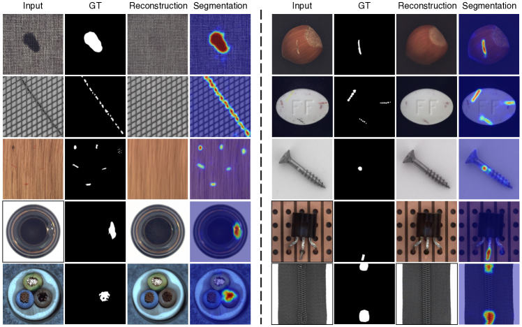
Figure 10: More qualitative examples on MVTec [4].

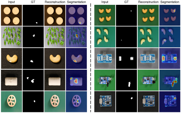
Figure 11: More qualitative examples on VisA [60].

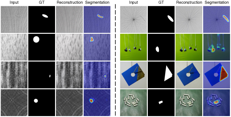
Figure 12: Qualitative examples on DAGM [52] and MPDD [22].

References

- Akcay et al. [2018] Samet Akcay, Amir Atapour-Abarghouei, and Toby P Breckon. Ganomaly: Semi-supervised anomaly detection via adversarial training. In ACCV, 2018.
- Baranchuk et al. [2021] Dmitry Baranchuk, Andrey Voynov, Ivan Rubachev, Valentin Khrulkov, and Artem Babenko. Label-efficient semantic segmentation with diffusion models. In ICLR, 2021.
- Baur et al. [2019] Christoph Baur, Benedikt Wiestler, Shadi Albarqouni, and Nassir Navab. Deep autoencoding models for unsupervised anomaly segmentation in brain mr images. In MICCAI, 2019.
- Bergmann et al. [2019] Paul Bergmann, Michael Fauser, David Sattlegger, and Carsten Steger. Mvtec ad–a comprehensive real-world dataset for unsupervised anomaly detection. In CVPR, 2019.
- Bergmann et al. [2020] Paul Bergmann, Michael Fauser, David Sattlegger, and Carsten Steger. Uninformed students: Student-teacher anomaly detection with discriminative latent embeddings. In CVPR, 2020.
- Brempong et al. [2022] Emmanuel Asiedu Brempong, Simon Kornblith, Ting Chen, Niki Parmar, Matthias Minderer, and Mohammad Norouzi. Denoising pretraining for semantic segmentation. In CVPR, 2022.
- Chen et al. [2023] Shoufa Chen, Peize Sun, Yibing Song, and Ping Luo. Diffusiondet: Diffusion model for object detection. In ICCV, 2023.
- Cimpoi et al. [2014] Mircea Cimpoi, Subhransu Maji, Iasonas Kokkinos, Sammy Mohamed, and Andrea Vedaldi. Describing textures in the wild. In CVPR, 2014.
- Cohen and Hoshen [2020] Niv Cohen and Yedid Hoshen. Sub-image anomaly detection with deep pyramid correspondences. arXiv preprint arXiv:2005.02357, 2020.
- Defard et al. [2021] Thomas Defard, Aleksandr Setkov, Angelique Loesch, and Romaric Audigier. Padim: a patch distribution modeling framework for anomaly detection and localization. In ICPR, 2021.
- Dehaene and Eline [2020] David Dehaene and Pierre Eline. Anomaly localization by modeling perceptual features. arXiv preprint arXiv:2008.05369, 2020.
- Dehaene et al. [2019] David Dehaene, Oriel Frigo, Sébastien Combrexelle, and Pierre Eline. Iterative energy-based projection on a normal data manifold for anomaly localization. In ICLR, 2019.
- Deng and Li [2022] Hanqiu Deng and Xingyu Li. Anomaly detection via reverse distillation from one-class embedding. In CVPR, 2022.
- Dhariwal and Nichol [2021] Prafulla Dhariwal and Alexander Nichol. Diffusion models beat gans on image synthesis. In NeurIPS, 2021.
- Girshick [2015] Ross Girshick. Fast r-cnn. In ICCV, 2015.
- Gong et al. [2019] Dong Gong, Lingqiao Liu, Vuong Le, Budhaditya Saha, Moussa Reda Mansour, Svetha Venkatesh, and Anton van den Hengel. Memorizing normality to detect anomaly: Memory-augmented deep autoencoder for unsupervised anomaly detection. In ICCV, 2019.
- Graikos et al. [2022] Alexandros Graikos, Nikolay Malkin, Nebojsa Jojic, and Dimitris Samaras. Diffusion models as plug-and-play priors. arXiv preprint arXiv:2206.09012, 2022.
- Gudovskiy et al. [2022] Denis Gudovskiy, Shun Ishizaka, and Kazuki Kozuka. Cflow-ad: Real-time unsupervised anomaly detection with localization via conditional normalizing flows. In WACV, 2022.
- He et al. [2016] Kaiming He, Xiangyu Zhang, Shaoqing Ren, and Jian Sun. Deep residual learning for image recognition. In CVPR, 2016.
- Ho et al. [2020] Jonathan Ho, Ajay Jain, and Pieter Abbeel. Denoising diffusion probabilistic models. In NeurIPS, 2020.
- Hou et al. [2021] Jinlei Hou, Yingying Zhang, Qiaoyong Zhong, Di Xie, Shiliang Pu, and Hong Zhou. Divide-and-assemble: Learning block-wise memory for unsupervised anomaly detection. In CVPR, 2021.
- Jezek et al. [2021] Stepan Jezek, Martin Jonak, Radim Burget, Pavel Dvorak, and Milos Skotak. Deep learning-based defect detection of metal parts: evaluating current methods in complex conditions. In ICUMT, 2021.
- Kim et al. [2022] Boah Kim, Yujin Oh, and Jong Chul Ye. Diffusion adversarial representation learning for self-supervised vessel segmentation. arXiv preprint arXiv:2209.14566, 2022.
- Kingma and Ba [2014] Diederik P Kingma and Jimmy Ba. Adam: A method for stochastic optimization. arXiv preprint arXiv:1412.6980, 2014.
- Lee et al. [2022] Sungwook Lee, Seunghyun Lee, and Byung Cheol Song. Cfa: Coupled-hypersphere-based feature adaptation for target-oriented anomaly localization. ACCESS, 2022.
- Li et al. [2021] Chun-Liang Li, Kihyuk Sohn, Jinsung Yoon, and Tomas Pfister. Cutpaste: Self-supervised learning for anomaly detection and localization. In CVPR, 2021.
- Lin et al. [2017] Tsung-Yi Lin, Priya Goyal, Ross Girshick, Kaiming He, and Piotr Dollár. Focal loss for dense object detection. In ICCV, 2017.
- Liu et al. [2020] Wenqian Liu, Runze Li, Meng Zheng, Srikrishna Karanam, Ziyan Wu, Bir Bhanu, Richard J Radke, and Octavia Camps. Towards visually explaining variational autoencoders. In CVPR, 2020.
- Liu et al. [2023a] Wenrui Liu, Hong Chang, Bingpeng Ma, Shiguang Shan, and Xilin Chen. Diversity-measurable anomaly detection. In CVPR, 2023a.
- Liu et al. [2023b] Xihui Liu, Dong Huk Park, Samaneh Azadi, Gong Zhang, Arman Chopikyan, Yuxiao Hu, Humphrey Shi, Anna Rohrbach, and Trevor Darrell. More control for free! image synthesis with semantic diffusion guidance. In WACV, 2023b.
- Liu et al. [2023c] Zhikang Liu, Yiming Zhou, Yuansheng Xu, and Zilei Wang. Simplenet: A simple network for image anomaly detection and localization. In CVPR, 2023c.
- Perlin [1985] Ken Perlin. An image synthesizer. ACM SIGGRAPH, 1985.
- Qin et al. [2022] Xuebin Qin, Hang Dai, Xiaobin Hu, Deng-Ping Fan, Ling Shao, and Luc Van Gool. Highly accurate dichotomous image segmentation. In ECCV, 2022.
- Ristea et al. [2022] Nicolae-Cătălin Ristea, Neelu Madan, Radu Tudor Ionescu, Kamal Nasrollahi, Fahad Shahbaz Khan, Thomas B Moeslund, and Mubarak Shah. Self-supervised predictive convolutional attentive block for anomaly detection. In CVPR, 2022.
- Rombach et al. [2022] Robin Rombach, Andreas Blattmann, Dominik Lorenz, Patrick Esser, and Björn Ommer. High-resolution image synthesis with latent diffusion models. In CVPR, 2022.
- Ronneberger et al. [2015] Olaf Ronneberger, Philipp Fischer, and Thomas Brox. U-net: Convolutional networks for biomedical image segmentation. In MICCAI, 2015.
- Roth et al. [2022] Karsten Roth, Latha Pemula, Joaquin Zepeda, Bernhard Schölkopf, Thomas Brox, and Peter Gehler. Towards total recall in industrial anomaly detection. In CVPR, 2022.
- Rudolph et al. [2021] Marco Rudolph, Bastian Wandt, and Bodo Rosenhahn. Same same but differnet: Semi-supervised defect detection with normalizing flows. In WACV, 2021.
- Rudolph et al. [2022] Marco Rudolph, Tom Wehrbein, Bodo Rosenhahn, and Bastian Wandt. Fully convolutional cross-scale-flows for image-based defect detection. In WACV, 2022.
- Salehi et al. [2021] Mohammadreza Salehi, Niousha Sadjadi, Soroosh Baselizadeh, Mohammad H Rohban, and Hamid R Rabiee. Multiresolution knowledge distillation for anomaly detection. In CVPR, 2021.
- Salimans et al. [2017] Tim Salimans, Andrej Karpathy, Xi Chen, and Diederik P Kingma. Pixelcnn++: Improving the pixelcnn with discretized logistic mixture likelihood and other modifications. In ICLR, 2017.
- Schlegl et al. [2017] Thomas Schlegl, Philipp Seeböck, Sebastian M Waldstein, Ursula Schmidt-Erfurth, and Georg Langs. Unsupervised anomaly detection with generative adversarial networks to guide marker discovery. In IPMI, 2017.
- Sohl-Dickstein et al. [2015] Jascha Sohl-Dickstein, Eric Weiss, Niru Maheswaranathan, and Surya Ganguli. Deep unsupervised learning using nonequilibrium thermodynamics. In ICML, 2015.
- Song et al. [2020] Jiaming Song, Chenlin Meng, and Stefano Ermon. Denoising diffusion implicit models. In ICLR, 2020.
- Song et al. [2021] Jouwon Song, Kyeongbo Kong, Ye-In Park, Seong-Gyun Kim, and Suk-Ju Kang. Anoseg: anomaly segmentation network using self-supervised learning. arXiv preprint arXiv:2110.03396, 2021.
- Song and Ermon [2019] Yang Song and Stefano Ermon. Generative modeling by estimating gradients of the data distribution. In NeurIPS, 2019.
- Song and Ermon [2020] Yang Song and Stefano Ermon. Improved techniques for training score-based generative models. In NeurIPS, 2020.
- Tao et al. [2022] Xian Tao, Xinyi Gong, Xin Zhang, Shaohua Yan, and Chandranath Adak. Deep learning for unsupervised anomaly localization in industrial images: A survey. TIM, 2022.
- Tien et al. [2023] Tran Dinh Tien, Anh Tuan Nguyen, Nguyen Hoang Tran, Ta Duc Huy, Soan Duong, Chanh D Tr Nguyen, and Steven QH Truong. Revisiting reverse distillation for anomaly detection. In CVPR, 2023.
- Ulutas et al. [2020] Tolga Ulutas, Muhammed Ali Nur Oz, Muharrem Mercimek, and Ozgur Turay Kaymakci. Split-brain autoencoder approach for surface defect detection. In ICECCE, 2020.
- Vaswani et al. [2017] Ashish Vaswani, Noam Shazeer, Niki Parmar, Jakob Uszkoreit, Llion Jones, Aidan N Gomez, Łukasz Kaiser, and Illia Polosukhin. Attention is all you need. In NeurIPS, 2017.
- Wieler and Hahn [2007] Matthias Wieler and Tobias Hahn. Weakly supervised learning for industrial optical inspection. 2007.
- Wyatt et al. [2022] Julian Wyatt, Adam Leach, Sebastian M Schmon, and Chris G Willcocks. Anoddpm: Anomaly detection with denoising diffusion probabilistic models using simplex noise. In CVPR Workshop, 2022.
- Yang et al. [2023] Minghui Yang, Peng Wu, and Hui Feng. Memseg: A semi-supervised method for image surface defect detection using differences and commonalities. Eng Appl Artif Intell, 2023.
- Ye et al. [2020] Fei Ye, Chaoqin Huang, Jinkun Cao, Maosen Li, Ya Zhang, and Cewu Lu. Attribute restoration framework for anomaly detection. TMM, 2020.
- Yu et al. [2020] Jongmin Yu, Du Yong Kim, Younkwan Lee, and Moongu Jeon. Unsupervised pixel-level road defect detection via adversarial image-to-frequency transform. In IV, 2020.
- Yu et al. [2021] Jiawei Yu, Ye Zheng, Xiang Wang, Wei Li, Yushuang Wu, Rui Zhao, and Liwei Wu. Fastflow: Unsupervised anomaly detection and localization via 2d normalizing flows. arXiv preprint arXiv:2111.07677, 2021.
- Zavrtanik et al. [2021] Vitjan Zavrtanik, Matej Kristan, and Danijel Skočaj. Draem-a discriminatively trained reconstruction embedding for surface anomaly detection. In ICCV, 2021.
- Zhang et al. [2023] Hui Zhang, Zuxuan Wu, Zheng Wang, Zhineng Chen, and Yu-Gang Jiang. Prototypical residual networks for anomaly detection and localization. In CVPR, 2023.
- Zou et al. [2022] Yang Zou, Jongheon Jeong, Latha Pemula, Dongqing Zhang, and Onkar Dabeer. Spot-the-difference self-supervised pre-training for anomaly detection and segmentation. In ECCV, 2022.