Background Matters: Enhancing Out-of-distribution Detection with Domain Features

Abstract

Detecting out-of-distribution (OOD) inputs is a principal task for ensuring the safety of deploying deep-neural-network classifiers in open-world scenarios. OOD samples can be drawn from arbitrary distributions and exhibit deviations from in-distribution (ID) data in various dimensions, such as foreground semantic features (e.g., vehicle images vs. ID samples in fruit classification) and background domain features (e.g., textural images vs. ID samples in object recognition). Existing methods focus on detecting OOD samples based on the semantic features, while neglecting the other dimensions such as the domain features. This paper considers the importance of the domain features in OOD detection and proposes to leverage them to enhance the semantic-feature-based OOD detection methods. To this end, we propose a novel generic framework that can learn the domain features from the ID training samples by a dense prediction approach, with which different existing semantic-feature-based OOD detection methods can be seamlessly combined to jointly learn the in-distribution features from both the semantic and domain dimensions. Extensive experiments show that our approach 1) can substantially enhance the performance of four different state-of-the-art (SotA) OOD detection methods on multiple widely-used OOD datasets with diverse domain features, and 2) achieves new SotA performance on these benchmarks.

1 Introduction

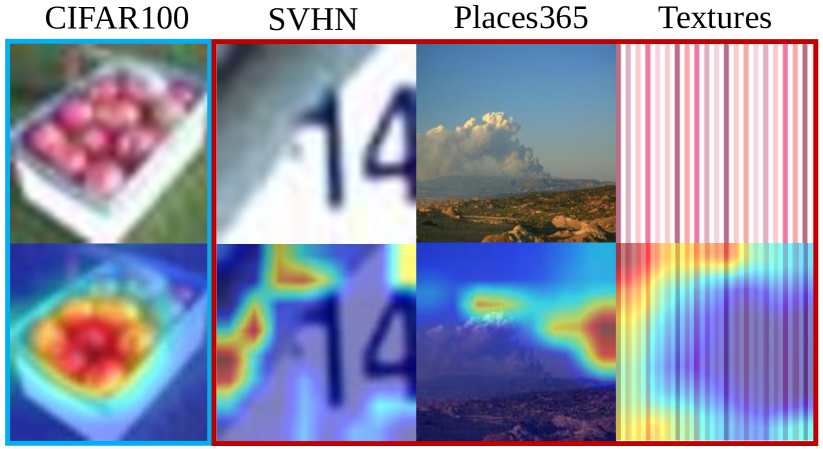
Figure 1: Example images in ID (CIFAR100 [21]) and OOD datasets (SVHN [29], Places365 [46], Textures [5]) with their attention maps from a classification network. The classifier focuses on the semantic features in the ID images and neglects the background domain features. It can mis-classify OOD samples that do not have clear semantics but have similar features to the ID classes.

Deep neural networks have demonstrated superior performance in computer vision tasks like classification and recognition [23]. Most deep learning methods assume that the training and test data are drawn from the same distribution. Thus, they fails to handle real-world scenarios with out-of-distribution (OOD) inputs that are not present in the training data [31]. Failures in distinguishing these OOD inputs from in-distribution (ID) data may lead to potentially catastrophic decisions, especially in safety-critical applications like autonomous driving or medical systems [4].

OOD detection approaches are designed to address this problem, which aim to detect and reject these OOD samples while guaranteeing the classification of in-distribution data [14]. There are generally two groups of OOD detection approaches. One of them are post-hoc approaches that work with a trained classification network to derive OOD scores without re-training or fine-tuning of the network, e.g., by using maximum softmax probability of the network outputs [14], maximum logits [13], or the Mahalanobis distance between the input and the class centroids of ID data [25]. Another group of approaches fine-tunes the classifiers with different methods, such as the use of pseudo OOD samples [15, 28, 27, 3, 30, 40, 42]. Most of these methods, especially the post-hoc methods, are focused to detect OOD samples based on the foreground semantic features, i.e., the features exhibiting the semantic of the in-distribution classes, such as the apple appearance features of ‘apples’ class images in CIFAR100 image classification shown in Fig. 1 (left). They, however, neglect the other dimensions that can also be important for OOD detection, since OOD samples can be drawn from arbitrary distributions and can exhibit deviations from in-distribution (ID) data in various dimensions. One of such dimensions is the set of background domain features that exhibit no class semantics. This is especially true for OOD samples that contain only small, or none, semantic patches, but have dominant domain features, such as the plates of house number, scenery or textual background in Fig. 1 (right). In such cases, semantic-feature-based OOD methods can misclassify these OOD samples to the classes with similar semantic features to these domain features.

This paper considers the importance of the domain features in OOD detection and proposes to leverage them to enhance semantic-feature-based OOD detection methods. To this end, we propose a novel generic framework called X-DOM that can learn the domain features from the ID training samples by a dense prediction approach, with which different existing semantic-feature-based OOD detection methods can be seamlessly combined to jointly learn the in-distribution features from both the semantic and domain dimensions. Specifically, given a trained $K$-class classification network where $K$ is the number of in-distribution classes, X-DOM first generates pseudo semantic segmentation masks by a weakly-supervised segmentation approach that uses image-level labels to locate discriminative regions in the images. These pseudo segmentation masks are then utilized to train a $(K+1)$-class dense prediction network, with the first $K$ classes being the original $K$ in-distribution classes and the $(K+1)$-th class corresponding to the in-distribution background domain features. The dense prediction network is further converted into a $(K+1)$-class classification network by adding a global pooling layer. The conversion is lossless and requires no re-training. In doing so, the $(K+1)$-class classifier learns both semantic and domain in-distribution features. Different existing semantic-feature-based methods, such as the post-hoc methods, can be applied to the first $K$ prediction outputs to obtain semantic OOD scores, while the $(K+1)$-th prediction can be directly used to define domain OOD scores. Combining these semantic and domain OOD scores enable the detection of OOD samples from both semantic and domain features.

In summary, we make the following main contributions:

• This work studies the importance of learning domain features and proposes to synthesize both domain and semantic features for more effective OOD detection in diverse real-world applications. This provides a new insight into the OOD detection problem.

• We then propose a novel generic approach X-DOM, in which different existing semantic-feature-based OOD detection methods can be seamlessly combined to jointly learn the in-distribution features from both semantic and domain dimensions. It offers a generic approach to enhance current OOD detection methods. To our knowledge, this is the first generic framework for joint semantic and domain OOD detection.

• We also introduce a weakly-supervised dense prediction method specifically designed to learn the in-distribution domain features for OOD detection.

• Extensive experiments on four widely-used OOD datasets with diverse domain features show that our approach X-DOM 1) can substantially enhance the performance of four different state-of-the-art (SotA) OOD detection methods, and 2) achieves new SotA performance on these benchmarks.

2 Related Work

Post-hoc Approaches. Modelling the uncertainty of pre-trained DNN networks directly without retraining the network is one popular approach for OOD detection [10, 6, 18, 33, 2, 38, 47]. Hendrycks et al. [14] propose the uncertainty of DNNs and establish a baseline for OOD detection by maximum softmax probability (MSP). ODIN [26] introduces input perturbation and temperature scaling to enhance MSP. Lee et al. [25] propose the deep Mahalanobis distance-based detectors, which compute the distance-based OOD scores from the pre-trained networks’ features. Liu et al. [27] calculate the logsunexp on logit as the energy OOD score. ReAct [34] reduces the DNN’s overconfidence in OOD samples by activation clipping, which further enhances the energy scores. MaSF [11] considers the empirical distribution of each layer and channel in the CNN and returns a p-value as the OOD score. Dong et al. [8] observe that the model activation averages for OOD and ID inputs are significantly distinct and compute the neural mean from the batch normalized layer for OOD detection. Recently, ViM [37] attempts to utilize not only primitive semantic features but also their residuals to define more effective logit-based OOD scores. This type of approach relies on the semantic features learned by the pre-trained networks, which neglects other relevant features, such as domain features.

Fine-tuning Approaches. Another dominant approach is to fine-tune the classification networks for adapting to the OOD detection tasks. In this line of research, Hsu et al. [17] further improve ODIN by decomposing confidence scoring. Zaeemzadeh et al. [43] project ID samples into a one-dimensional subspace during training. Some other studies [36, 19] group ID data and assume them as OOD samples for each other to guide the network training. Outlier Exposure (OE) [15] introduces auxiliary outlier data to train the network and improve its OOD detection performance. Such approaches can use real outliers [28, 27, 3, 30, 40, 42] or synthetic ones from generative models [24]. The performance of this approach often depends on the quality of the outlier data. Fine-tuning the networks may also lead to the loss of semantic information and consequently degraded classification accuracy on the ID data. Our method does not require additional outliers and can retain the semantic information of the ID data during training.

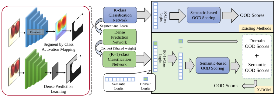
Figure 2: Overview of our proposed framework. It first uses a trained $K$-class classification network to obtain pseudo semantic segmentation masks and then learns the in-distribution features by training a $(K+1)$-class classification network with the pseudo labels (Left). It lastly converts the dense prediction network to a $(K+1)$-class classifier in a lossless fashion, and leverages these $(K+1)$ prediction outputs for joint semantic and domain OOD detection (Bottom Right).

3 Proposed Approach

Problem Statement. Given a set of training samples $\mathcal{X}=\{\mathbf{x}_{i},y_{i}\}_{i=1}^{N}$ drawn from an in-distribution $\mathit{P}_{\mathcal{X}}$ with label space $\mathcal{Y}=\{y_{j}\}_{j=1}^{K}$, and let $f:\mathcal{X}\rightarrow\mathbb{R}^{\mathcal{Y}}$ be a classifier trained on the in-distribution samples $\mathcal{X}$, then the goal of OOD detection is to obtain a new decision function $g$ to discriminate whether $\mathbf{x}$ come from $\mathit{P}_{\mathcal{X}}$ or out-of-distribution data $\mathit{P}_{out}$:

$$g(\mathbf{x},f)=\left\{\begin{array}[]{l}1\quad\text{if}\enspace\mathbf{x}\in\mathit{P}_{out},\\ 0\quad\text{if}\enspace\mathbf{x}\in\mathit{P}_{\mathcal{X}}.\end{array}\right.$$

The difference between $\mathit{P}_{\mathcal{X}}$ and $\mathit{P}_{out}$ determines the difficulty of detecting the OOD samples. Existing OOD detection approaches focus on the difference between $\mathit{P}_{\mathcal{X}}$ and $\mathit{P}_{out}$ based on the semantic information of the class label space $\mathcal{Y}$, neglecting other relevant dimensions such as the background domain feature space. This work aim to learn the domain features and leverage them to complement these semantic-feature-based OOD detection approaches.

3.1 Overview of Our Approach

Using semantic features only to detect OOD samples can often be successful when the OOD samples have some dominant semantics that are different from the ID images. However, this type of approach would fail to work effectively when the OOD samples do not have clear semantics and/or exhibit some similar semantic appearance to the ID samples, e.g., the images illustrated in Fig. 1. Motivated by this, we introduce a generic framework X-DOM, in which the model learns the background domain features of the in-distribution data, upon which different existing OOD detection methods can be applied with the learned domain feature representations to detect OOD samples from both of the semantic and domain feature dimensions. A high-level overview of our proposed framework is provided in Fig. 2.

1. X-DOM first learns the in-distribution domain features by a $(K+1)$-class dense prediction network trained from the given pre-trained K-class classification network.

2. It then seamlessly integrates the domain features into image classification models by transforming the dense prediction network to a $(K+1)$-class classification network, where the prediction entries of the $K$ classes are focused on the class semantics of the $K$ in-distribution class while the extra (+1) class is focused on the in-distribution domain features.

3. Lastly, an OOD score in the semantic dimension obtained from existing post-hoc OOD detectors based on the $K$-class predictions, and an OOD score obtained from the extra (+1) class prediction from the domain dimension, are synthesized to perform OOD detection.

3.2 Learning In-distribution Domain Features via $(K+1)$-class Dense Prediction

X-DOM aims to explicitly learn representations of the image background information as in-distribution domain features. The key challenge here is how to locate these background domain features and separate them from the foreground semantic features. We introduce a weakly-supervised dense prediction method to tackle this challenge, in which weakly-supervised semantic segmentation methods are first utilized to generate pseudo segmentation mask labels that are then used to train a $(K+1)$-class dense prediction network. The extra (+1) class learned in the dense predictor is specifically designed to learn the in-distribution features, while the other $K$ class predictions are focused on learning the semantic features of the $K$ classes given in the training data. Particularly, given the training data $\mathcal{X}$ with $K$-class image-level labels $\mathcal{Y}$ and a trained $K$-class classification network $\phi$, the pseudo segmentation mask labels can be obtained by the class activation mapping [45]:

$$\mathbf{M}_{y_{\mathbf{x}}}^{(i,j)}=\mathbf{W}_{y_{\mathbf{x}}}^{\top}\phi_{\text{cnn}}(\mathbf{x})^{(i,j)},$$ (1)

where $\mathbf{W}_{y_{\mathbf{x}}}$ is the classification weight of the trained classifier $\phi$ corresponding to the groundtruth class $y_{\mathbf{x}}$ of $\mathbf{x}$, and $\phi_{\text{cnn}}(\mathbf{x})^{(i,j)}$ obtains the feature vector at the unit $(i,j)$ in the feature map extracted by the feature extractor in $\phi$ from image $\mathbf{x}$. $\mathbf{M}_{y_{\mathbf{x}}}\in\mathbb{R}^{H\times W}$ is an attention map indicating a pixel-wise semantic score of $\mathbf{x}$ relative to its groundtruth class $y_{\mathbf{x}}$. We then define a foreground decision threshold $\theta$ to generate the fine-grained pseudo labels of background domain pixels and foreground semantic pixels by:

$$\mathbf{\hat{Y}}^{(i,j)}(\mathbf{x})=\left\{\begin{array}[]{ll}0&\text{if}\;\mathbf{M}_{y_{\mathbf{x}}}^{(i,j)}<\theta,\\ 1&\text{if}\;\mathbf{M}_{y_{\mathbf{x}}}^{(i,j)}\geqslant\theta,\end{array}\right.$$ (2)

where the attention scores are normalized into the range $[0,1]$ and $\theta=0.5$ is used. We then leverage these pseudo labels of the domain and semantic pixels, $\mathbf{\hat{Y}}$, to train a $(K+1)$-class dense prediction network $f_{\Theta_{d}}:\mathcal{X}\rightarrow\{0,1\}^{K\times H\times W}$ via a pixel-level cross entropy loss:

$$L(\mathbf{x},\mathbf{\hat{Y}})=\frac{-1}{H\times W}\sum_{i=1}^{H}\sum_{j=1}^{W}\sum_{k=1}^{K+1}\hat{y}_{k}^{(i,j)}\log\left(f(\mathbf{x},\Theta_{d})_{k}^{(i,j)}\right),$$ (3)

where $f(\mathbf{x},\Theta_{d})^{(i,j)}$ outputs a prediction vector consisting of prediction probabilities of the $K+1$ classes at the image pixel $(i,j)$, and $\hat{\mathbf{y}}^{(i,j)}$ denotes the corresponding pseudo labels at the same pixel. In doing so, $f_{\Theta_{d}}$ learns both in-distribution semantic and domain features.

3.3 Dense Prediction to Image Classification

The pixel-level semantic and domain features learned in the dense prediction network cannot be applied directly to the image classification task. We show below that the $(K+1)$-class dense prediction network can be transformed to a $(K+1)$-class image classification network in a lossless fashion: the dense prediction and the classification networks share the same weight parameters, and the classification network can be applied to image classification without re-training. Particularly, the dense prediction network $f_{\Theta_{d}}:\mathcal{X}\rightarrow\{0,1\}^{K\times H\times W}$ can be decomposed into three main modules: 1) a feature extraction network $f_{\Theta_{\mathit{CNN}}}:\mathcal{X}\rightarrow\mathcal{G}$ consisting of a convolutional neural network that extracts the input image $\mathbf{x}\in\mathbb{R}^{3\times H\times W}$ into a smaller scale but larger dimensional feature map $\mathbf{G}\in\mathbb{R}^{C\times h\times w}$, 2) an upsampling module $\text{up}(\cdot)$ that upsamples the feature map $\mathbf{G}$ to original input size $H\times W$, typically implemented using bilinear interpolation, and 3) a 1x1 convolution classifier $f_{\Theta_{\mathit{cls}}}:\mathcal{G}\rightarrow\mathcal{L}$ that computes the logit for each pixel in the feature map and outputs a logit map $\mathbf{L}\in\mathbb{R}^{K\times H\times W}$. The size of weights of the convolutional classifier is $C\times(K+1)$. Thus, the dense prediction network $f_{\Theta_{d}}$ can be denoted as:

$$f(\mathbf{x},\Theta_{d})=\text{softmax}(f(\text{up}(f(\mathbf{x},\Theta_{\mathit{CNN}})),\Theta_{\mathit{cls}})),$$ (4)

where $\Theta_{d}=\{\Theta_{\mathit{CNN}},\Theta_{\mathit{cls}}\}$.

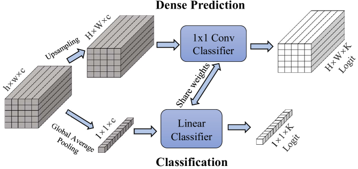
Figure 3: Lossless conversion of a dense prediction network to a classification network.

For a classification network $f_{\Theta_{c}}:\mathcal{X}\rightarrow\mathbb{R}^{\mathcal{Y}}$, it can be similarly decomposed into three main modules: 1) a feature extraction network $f_{\Theta_{\mathit{CNN}}}:\mathcal{X}\rightarrow\mathcal{G}$ with the same function as the dense prediction network, 2) a global average pooling $\text{GAP}(\cdot)$, which compresses the feature map of $C\times H\times W$ into a feature vector of size $C\times 1\times 1$, integrating the features of the full image, and 3) a linear classifier $f_{\Theta_{\mathit{cls}}}:\mathcal{G}\rightarrow\mathcal{L}$, which computes the logit of the full image based on the feature vector with $C\times(K+1)$ weights. The classification network $f_{\Theta_{c}}$ can be denoted as:

$$f(\mathbf{x},\Theta_{c})=\text{softmax}(f(\text{GAP}(f(\mathbf{x},\Theta_{\mathit{CNN}})),\Theta_{\mathit{cls}})),$$ (5)

where $\Theta_{c}=\{\Theta_{\mathit{CNN}},\Theta_{\mathit{cls}}\}$. It is clear from Eqs. (4) and (5) that the only difference between $f_{\Theta_{d}}$ and $f_{\Theta_{c}}$ is the upsampling module and the GAP module, sharing the same feature extraction network and the classifier. Further, the upsampling and the GAP modules are weight-free operations, which can be easily replaced with each other, as shown in Fig. 3. In this way, we directly transfer the in-distribution semantic and domain features learned in the dense prediction network $f_{\Theta_{d}}$ to the image classification network $f_{\Theta_{c}}$ without any loss of the wegith parameters learned in $f_{\Theta_{d}}$. For a given test image, the classifier $f_{\Theta_{c}}$ yields a $(K+1)$-dimensional logit vector, where the $(K+1)$-th logit is focused on the in-distribution domain features and can be used directly to detect OOD samples from the domain dimension:

$$S_{d}(\mathbf{x})=\mathbf{l}_{\mathbf{x}}(K+1),$$ (6)

where $\mathbf{l}_{\mathbf{x}}=f(\text{GAP}(f(\mathbf{x},\Theta_{\mathit{CNN}})),\Theta_{\mathit{cls}})$ is a (K+1)-dimensional prediction logit vector yielded by $f_{\Theta_{c}}$.

3.4 Joint Semantic and Domain OOD Detection

Although the domain-feature-based OOD score $S_{d}$ can be used to detect OOD samples directly, it can miss the OOD samples whose detection relies heavily on the semantic features. Thus, we propose to utilize this domain OOD score to complement existing SotA semantic-feature-based OOD detectors. Particularly, since the first $K$ classification logits in $f_{\Theta_{c}}$ capture similar class semantics as the original $K$-class classifier, off-the-shelf post-hoc OOD detection methods that derive an OOD score from these $K$ classification logits can be plugged into X-DOM to obtain an OOD score from the semantic feature aspect. These domain and semantic feature-based OOD scores are synthesized to achieve a joint semantic and domain OOD detection.

There are generally two types of post-hoc OOD detection approaches, including raw logit-based and softmax probability-based methods. Our domain-feature-based OOD score is based on an unbounded logit value, which can dominant the overall OOD score when combining with the semantic-feature-based OOD score using the softmax output (its value is within $[0,1]$). To avoid this situation, we take a different approach to combine the domain and semantic feature-based OOD scores, depending on the type of the semantic-feature-based OOD detector used:

$$S(\mathbf{x})=\left\{\begin{array}[]{ll}S_{h}(\mathbf{x})+\frac{\log(S_{d}(\mathbf{x}))}{T}&\text{if}\;S_{h}\;\text{is softmax-based},\\ S_{h}(\mathbf{x})+\frac{S_{d}(\mathbf{x})}{T}&\text{if}\;S_{h}\;\text{is logit-based},\end{array}\right.$$ (7)

where $S(\mathbf{x})$ is the final OOD score used to perform OOD detection in X-DOM, $S_{h}(\mathbf{x})=h(\mathbf{x})$ denotes the OOD score obtained from using an existing semantic-feature-based OOD scoring function $h$, and $T$ is a temperature coefficient hyperparameter. In Eq. (7), to obtain faithful semantic-and-domain-combined OOD score, the log function is used to constrain the value and the variance of the domain scores $S_{d}$, while $T$ is used to adjust the distribution of the domain scores to match that of the semantic scores.

4 Experiments

Datasets. Following [14, 26, 25, 27, 11, 8] , we choose two widely used classification datasets: CIFAR10 and CIFAR100 [21], as the in-distribution datasets. As OOD samples are unknown during training, their respective training and test data are used as ID data, with samples from a different dataset added into the test set as the OOD data. To evaluate the effectiveness of our approach, four commonly-used OOD datasets consisting of natural image datasets with diverse background domain features are used, including SVHN [29], Places365 [46], Textures [5], and CIFAR100/CIFAR10 [21] (CIFAR100 is used as OOD data when CIFAR10 is used as ID data, and vise versa [9, 32, 33]) SVHN is a digit classification dataset cropped from pictures of house number plates, Places365 is a large-scale scene classification dataset, while Textures contains 5,640 texture images in the wild that do not contain specific objects and backgrounds. Images in all these three datasets exhibit largely different semantic and domain distributions, so the three datasets contain strong out-of-distribution semantic and domain features. On the other hand, both CIFAR10 and CIFAR100 are sampled from Tiny Images [35] and they share similar domain features, so when they are used as OOD data for each other, the domain features are weak. Also, the objects in the images of these two datasets can be very similar, so the semantic OOD features are also weak. As a result, this pair of mutual OOD/ID combination is considered as hard OOD detection benchmarks [39]

Table 1: OOD detection results with CIFAR10 as in-distribution data. All methods are based on ID training data without using any external outlier data. ^† indicates that the results are taken from the original paper, and other methods are reproduced using the same network architecture. Four post-hoc semantic OOD detection methods are respectively plugged into our method X-DOM, with improved results highlighted in red and in blue otherwise. The best result per dataset is boldfaced.

Methods	OOD Datasets				Average
	CIFAR100	SVHN	Places365	Textures
	FPR95$\downarrow$ /AUROC$\uparrow$ /AUPR$\uparrow$
MaxLogit [13] [ICML’22]	39.11/85.07/78.13	17.95/94.78/84.22	24.05/91.10/86.41	7.93/97.57/98.07	22.26/92.13/86.71
KL-Matching [13] [ICML’22]	33.63/90.20/88.18	25.70/95.21/88.37	25.25/92.88/90.78	12.61/97.28/98.21	24.30/93.89/91.38
ReAct [34] [NIPS’21]	34.75/84.10/79.89	20.03/90.58/76.30	23.45/91.88/89.43	10.27/96.53/97.69	22.12/90.77/85.83
MaSF† [11] [ICLR’22]	- /82.10/ -	- /99.80/ -	- /96.00/ -	- /98.50/ -	- /94.10/ -
NMD† [8] [CVPR’22]	- /90.10/ -	- /99.60/ -	- / - / -	- /98.90/ -	- /72.15/ -
MSP [14] [ICLR’17]	33.44/89.01/84.10	17.40/95.72/88.68	22.47/92.93/89.79	8.55/97.66/98.38	20.46/93.83/90.24
MSP-DOM [Ours]	23.75/94.29/93.48	2.55/98.94/97.88	5.05/98.49/98.60	0.02/99.90/99.95	7.84/97.90/97.48
ODIN [26] [ICLR’18]	34.62/87.83/81.92	16.13/95.66/87.30	22.15/92.43/88.59	7.45/97.86/98.37	20.09/93.45/89.04
ODIN-DOM [Ours]	22.15/95.50/95.29	4.27/99.19/98.30	8.08/98.66/98.76	0.34/99.92/99.95	8.71/98.32/98.07
Energy [27] [NIPS’20]	41.98/84.25/77.47	19.73/94.46/83.67	25.42/90.74/86.06	8.72/97.45/97.99	23.96/91.73/86.30
Energy-DOM [Ours]	19.90/94.98/93.76	3.10/99.28/98.14	6.96/98.60/98.52	0.53/99.87/99.91	7.62/98.19/97.58
ViM [37] [CVPR’22]	15.25/96.92/96.78	1.27/99.47/99.08	2.74/99.32/99.34	0.11/99.93/99.96	4.84/98.91/98.79
ViM-DOM [Ours]	13.49/97.08/96.75	0.41/99.85/99.68	0.72/99.85/99.85	0.00/100.00/100.00	3.65/99.20/99.07

Table 2: OOD detection results with CIFAR100 as in-distribution data. The notations here are the same as that in Tab. 1.

Methods	OOD Datasets				Average
	CIFAR10	SVHN	Places365	Textures
	FPR95$\downarrow$ /AUROC$\uparrow$ /AUPR$\uparrow$
MaxLogit [13] [ICML’22]	61.61/81.09/79.25	37.12/91.29/80.77	71.89/73.12/67.64	37.61/90.63/93.73	52.06/84.03/80.35
KL-Matching [13] [ICML’22]	64.49/79.54/74.46	47.86/89.08/76.63	73.55/78.04/76.61	46.63/88.97/92.16	58.13/83.91/79.96
ReAct [34] [NIPS’21]	70.81/79.62/78.97	53.00/88.88/78.43	82.64/68.11/63.28	52.80/88.15/92.58	64.81/81.19/78.31
MaSF† [11] [ICLR’22]	- /64.00/ -	- /96.90/ -	- /81.10/ -	- /92.00/ -	- /83.50/ -
MSP [14] [ICLR’17]	64.25/81.52/80.87	49.50/88.92/79.07	72.10/76.18/71.52	46.24/89.33/93.44	58.02/83.99/81.23
MSP-DOM [Ours]	58.76/84.67/84.25	50.75/89.27/82.39	67.82/85.20/88.06	28.21/95.86/97.85	51.38/88.75/88.14
ODIN [26] [ICLR’18]	59.67/82.39/80.79	38.11/91.32/81.40	69.80/75.39/69.81	37.38/91.10/94.22	51.24/85.05/81.55
ODIN-DOM [Ours]	55.92/87.31/88.02	32.79/90.60/76.03	55.34/81.56/79.62	10.78/97.40/98.23	38.71/89.22/85.48
Energy [27] [NIPS’20]	64.34/80.48/78.89	36.76/91.38/80.98	74.75/72.14/67.10	39.17/90.37/93.61	53.75/83.59/80.15
Energy-DOM [Ours]	54.02/88.12/88.82	24.78/93.39/81.94	48.87/85.72/82.67	7.11/98.41/98.92	33.70/91.41/88.09
ViM [37] [CVPR’22]	59.13/85.72/85.87	10.23/97.90/95.74	49.38/87.23/86.19	2.45/99.47/99.69	30.30/92.58/91.87
ViM-DOM [Ours]	60.88/85.74/86.38	7.58/98.40/96.39	20.93/96.06/96.23	0.16/99.96/99.98	22.39/95.04/94.74

Implementation Details. We use BiT-M [20], a variant of ResNetv2 architecture [12], as the default network backbone throughout the experiments. The official release checkpoint of BiT-M-R50x1 trained on ImageNet-21K is used as our initial $K$-class in-distribution classification model. The model is further fine-tuned on the in-distribution dataset (CIFAR10/CIFAR100) with 20,000 steps using a batch size of 128. SGD is used as the optimizer with an initial learning rate of 0.003 and a momentum of 0.9. We decay the learning rate by a factor of 10 at 30%, 60%, and 90% of the training steps. All images were resized to 160x160 and randomly cropped to 128x128. The Mixup [44] with $\alpha=0.1$ is also used to synthesize new image samples during training. We subsequently use CAM (Class Activation Mapping) [45] to generate the pseudo mask labels for each in-distribution image based on a multi-scale masking method used in [1] (see Appendix A.1 for the example of pseudo mask).

With these pseudo mask labels, we then use a modified Dense-BiT architecture to train the $(K+1)$-class dense prediction model with the BiT-M-R50x1 checkpoints as the initial weights. All input images are resized to 128x128 during training and inference. We replace the Mixup augmentation used in the training with randomly scaling (from 0.5 to 2.0) and randomly horizontally flipping augmentation. The other training strategy and hyperparameters are maintained the same as the ones used in training the $K$-class classification network above. After that, the dense prediction model is converted to $(K+1)$-class image classification model using Eq. (5).

Four post-hoc OOD detection methods, including MSP [14], ODIN [26], Energy [27], and ViM [37], are used as the plug-in base models. They are respectively employed to combine with X-DOM to detect OOD samples in both of semantic and domain features. To have fair and straightforward comparison, these four plug-in models are built upon the same $K$-class classification model as X-DOM. The temperature $T=2.5$ is used in Eq. (7) by default.

We will release our code upon paper acceptance.

Evaluation Metrics. We use three widely-used evaluation metrics for OOD detection, including: 1) FPR95 that evaluates the false positive rate of the OOD samples when the true positive rate of the in-distribution samples is 95%, 2) AUROC denotes the Area Under the Receiver Operating Characteristic curve, and 3) AUPR is the Area under the Precision-Recall curve. The ID images are the positive samples in calculating AUROC and AUPR to measure the OOD detection performance. In addition, we also report the Top-1 accuracy of classifying the in-distribution samples.

4.1 Main Results

The OOD detection results of X-DOM and its competing methods with CIFAR10 and CIFAR100 as in-distribution data are reported in Tabs. 1 and 2, respectively. Overall, X-DOM substantially improves four different SotA detection methods in all three evaluation metrics on both datasets, and obtains new SotA performance. We discuss the results in detail as follows.

Enhancing Different OOD Detection Methods. Four different SotA methods – MSP, ODIN, Energy, and ViM – are used as semantic-feature-based OOD detection baseline models and plugged into X-DOM to perform joint semantic and domain OOD detection. Their results are shown at the bottom of Tabs. 1 and 2.

Compared to all the four plug-in base models, X-DOM can significantly improve the performance of all evaluation metrics in terms of the average results over the four OOD datasets on both of the CIFAR10 and CIFAR100 datasets. In particular, for the averaged improvement across the four base models, X-DOM boosts the FPR95 by $10.38\%$, the AUROC by $3.92\%$ and the AUPR by $6.96\%$ AUPR in Tab. 1; and similarly, it boosts the FPR95 by $11.78\%$ , the AUROC by $4.8\%$ and the AUPR by $5.41\%$ in Tab. 2. Note that even for the base model ViM, the most recent SotA method, X-DOM can still considerably enhance its performance, especially on some datasets where ViM does not work well, such as the SVHN, Places365, and Textures datasets, resulting in over 6% reduction in FPR95 and 2.5% increase in both AUROC and AUPR on the CIFAR100 data. X-DOM shows slight performance drops on some metrics of CIFAR and SVHN OOD datasets, which are mainly caused by suboptimal combinations of the domain and semantic OOD scores with the default temperature setting. The explanation would be discussed in detail using Fig. 10 in Sec. 4.2.

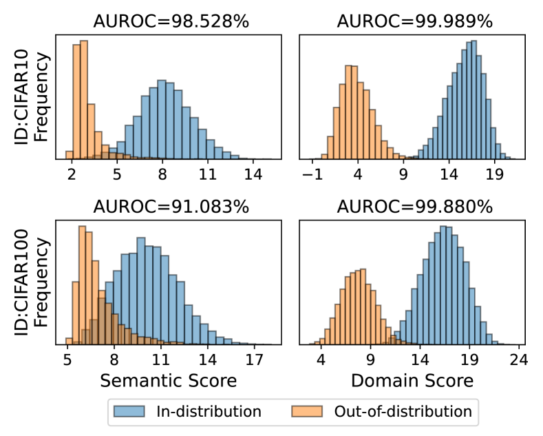
Figure 4: Distribution of the semantic/domain OOD scores of ID (CIFAR10/100) and OOD samples (Textures) in X-DOM.

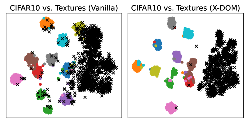
Figure 5: t-SNE visualization of the features learned by the vanilla classification network and X-DOM, where the colored dots are ID samples of different classes, and the black $\times$ are OOD samples.

Comparison to SotA Methods. X-DOM is also compared with five very recent SotA methods, including MaxLogit [13], KL-Matching [13], ReAct [34], MaSF [11] and NMD [8] , with their results reported at the top of Tabs. 1 and 2. Among all our four X-DOM methods and the SotA methods, ViM-DOM is consistently the best performer except the CIFAR10 data in Tab. 2 where Energy-DOM is the best detector. This is mainly because the ViM is generally the best semantic-feature-based OOD scoring method, and X-DOM can perform better when the plug-in base model is stronger. Further, it is impressive that although the base models MSP, ODIN and Energy that largely underperform the SotA competing methods, X-DOM can significantly boost their performance and outperform these SotA competing methods on nearly all cases in Tabs. 1 and 2.

The Reasons behind the Effectiveness of X-DOM. We aim to understand the effectiveness of X-DOM from two perspectives, including the domain and semantic OOD scoring, and the latent features learned in X-DOM, with the results on the Textures dataset reported in Figs. 4 and 5 respectively. We can see in Fig. 4 that the domain OOD scores in X-DOM enable a significantly better ID and OOD separation than the semantic OOD scores, indicating that the ID and OOD samples can be easier to be separated by looking from the domain features than the semantic features since there can be more background domain regions/pixels than the foreground semantic ones in each ID/OOD image. From the feature representation perspective, compared to the features learned in the vanilla $K$-class classifier in Fig. 5 (left), the features learned by the $(K+1)$-class classifier in X-DOM (Fig. 5 (right)) are more discriminative in distinguishing OOD samples from ID samples. This may be due to that training the classifier using fine-grained pixel-wise class labels helps learn better semantic features, in addition to the learning of the domain features.

4.2 Ablation Study

Table 3: FPR95 Results of X-DOM and its variants.

Module		DOM	Energy	Energy-DOM	ViM	ViM-DOM
$S_{h}$			$\checkmark$	$\checkmark$	$\checkmark$	$\checkmark$
$S_{d}$		$\checkmark$		$\checkmark$		$\checkmark$
CIFAR10	CIFAR100	38.16	41.98	19.90	15.25	13.49
	SVHN	2.60	19.73	3.10	1.27	0.41
	Places365	4.40	25.42	6.96	2.74	0.72
	Textures	0.04	8.72	0.53	0.11	0.00
	Average	11.30	23.96	7.62	4.84	3.65
CIFAR100	CIFAR10	89.24	64.34	54.02	59.13	60.88
	SVHN	26.61	36.76	24.7	10.23	7.58
	Places365	26.55	74.75	48.87	49.38	20.93
	Textures	0.53	39.17	7.11	2.45	0.16
	Average	35.73	53.75	33.70	30.30	22.39

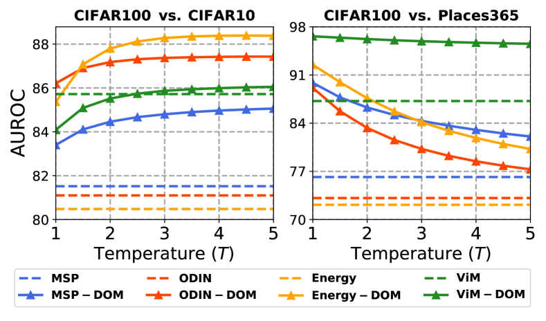
Figure 6: AUROC results of X-DOM using varying $\mathit{T}$ settings.

Domain OOD Score $S_{d}$ and the Joint OOD Score $S$. Tab. 5 shows the FPR95 results of OOD scoring methods in our model, including the use of domain OOD scores $S_{d}$ only (DOM), semantic OOD scores $S_{h}$ (Energy and ViM are used), and the full X-DOM model (See Appendix C.1 for more detailed results). Compared to the two semantic OOD scoring methods, Energy and ViM, using only the domain OOD scoring $S_{d}$ in X-DOM can obtain significantly reduced FPR95 errors, especially on OOD benchmarks such as Places356 and Textures where significant domain differences are presented compared to the in-distribution domain. This demonstrates that X-DOM can effectively learn the in-distribution domain features that can be used to detect OOD samples from the background domain aspect. Nevertheless, DOM works less effectively on the benchmark CIFAR100 vs. CIFAR10 where the domain difference is weak and detecting OOD samples rely more on the semantic features. In such cases, the full X-DOM models – Energy-DOM and ViM-DOM – that synthesize semantic OOD scores $S_{h}$ and domain OOD scores $S_{d}$ are needed; they significantly outperform the separate domain/semantic OOD scoring methods across the datasets.

Temperature $T$ in Synthesizing Domain and Semantic OOD Scores. One key challenge in plugging existing semantic OOD scores into X-DOM in Eq. (7) is the diverse range of different semantic OOD scores yielded by the existing methods. Fig. 10 the variants of X-DOM of using different temperature $T$ values to study the effects (see Appendix C.2 for the results on the other datasets). We can observe that the performance of all methods in CIFAR100 vs. CIFAR10 gradually improves as the temperature increases. This is because the increase of $T$ narrows down the distribution of domain scores, thus making the final OOD scores emphasizing more on the semantic OOD scores, which are more effective in the OOD datasets like CIFAR100 (ID) vs. CIFAR10 (OOD) where the domain difference is very small. In contrast, the performance of all methods in CIFAR100 (ID) vs. Places365 (OOD) gradually decreases as the temperature increases. This is because the domain distribution difference dominates over the semantic difference in such cases, on which enlarging the distribution of domain OOD scores is more effective. $T=2.5$ is generally a good trade-off of the domain and semantic OOD scores, and it is thus used by default in X-DOM. Note that adjusting $T$ generally does not bring the overall performance down below the baseline performance, showing the effectiveness of X-DOM using different $T$ values.

4.3 Further Analysis of X-DOM

Table 4: Top-1 accuracy results of in-distribution classification. Vanilla is the primitive trained classification network $\phi$ in Sec. 3.2.

Method	CIFAR10	CIFAR100
Vanilla	97.25%	85.94%
X-DOM	97.13%	86.17%

In-distribution Classification Accuracy. A potential risk of modifying the primitive classification network for OOD detection is the large degradation of the in-distribution classification accuracy. As shown in Tab. 4, our proposed X-DOM does not have this issue, as X-DOM has only 0.12% top-1 accuracy drop on the CIFAR10 dataset and improves the classification performance by 0.23% on the CIFAR100 dataset. This result indicates that the dense prediction training in X-DOM ensures effective learning of semantic features, while learning the domain features. The 0.23% accuracy increase on CIFAR100 also indicates that the dense prediction task can also improve the semantic feature learning for in-distribution classification.

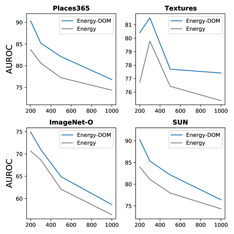
Figure 7: AUROC results of X-DOM and the Energy baseline in large-scale semantic space using ImageNet-1k as ID data.

Extending to Large-scale Semantic Space. A further challenge for OOD detection is on datasets with a large number of ID classes and high-resolution images, e.g., ImageNet-1k [7]. Fig. 7 presents the detection performance of X-DOM using ImageNet-1k as in-distribution dataset and on four OOD datasets, including two new high resolution datasets, ImageNet-O [16] and SUN [41]. To examine the impact of the number of classes, we show the results using $\mathit{C}\in\{200,300,500,1000\}$ randomly selected ID classes from ImageNet-1k ($C=1000$ is the full ImageNet-1k data; see Appendix B.2 for more details). The results show that X-DOM can consistently and significantly outperform its base model Energy with increasing number of ID classes on four diverse OOD datasets, indicating the effectiveness of X-DOM working in large-scale semantic space. On the other hand, as expected, both Energy and X-DOM are challlenged by the large semantic space, and thus, their performance decreases with more ID classes. Extending to large-scale semantic space is a general challenge for existing OOD detectors. We leave it for future work.

5 Conclusions

In this paper, we reveal the importance of the background domain features for OOD detection that are neglected in current approaches. We further propose a novel OOD detection framework X-DOM that utilizes dense prediction networks to learn the in-distribution domain features from in-distribution training data. It then leverages these domain features to define domain OOD scores and seamlessly combines them with existing semantic-feature-based OOD methods to detect OOD samples from both domain and semantic aspects. Comprehensive results on popular OOD benchmarks with diverse background features show that X-DOM can significantly improve the detection performance of four different existing methods. Through this work, we promote the design of OOD detection algorithms focusing features beyond the semantic features to achieve more holistic OOD detection in real-world applications.

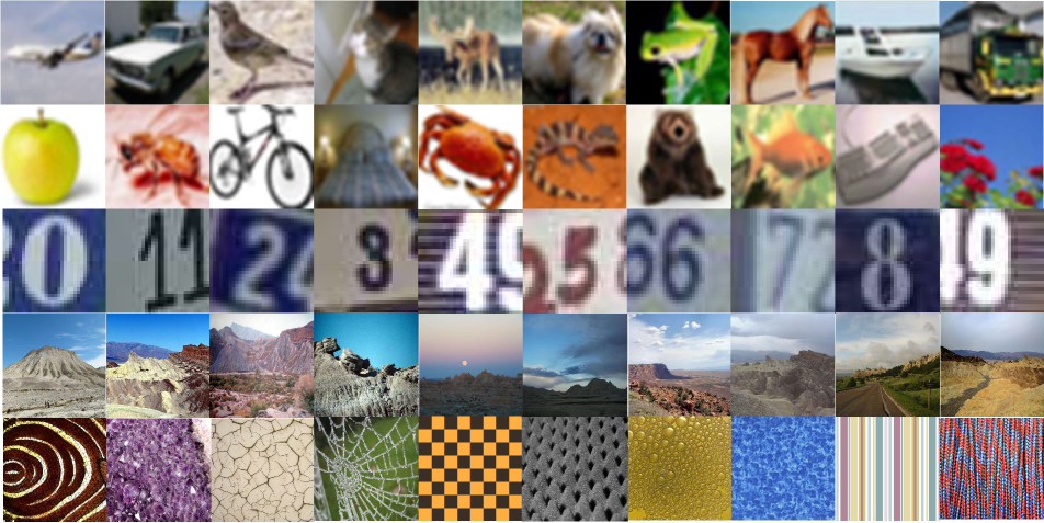
Figure 8: Example images of the five datasets we used. The rows from the top to the bottom are images from CIFAR10 [21], CIFAR100 [21], SVHN [29], Places365 [46], and Textures [5], respectively.

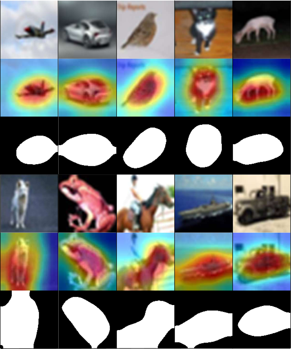
Figure 9: Examples of ID samples, CAMs, and pseudo-masks for CIFAR10. For each group of examples (three rows per group), the images on the top are original image, the middle is its class activate mapping visualisation, and the bottom ones are its pseudo-mask.

Table 5: Ablation results. ‘DOM’ is our method that uses only the domain OOD score, while ‘Vanilla X’ means the use of original semantic OOD scoring function in the method X. Best results in each group are highlighted.

Methods	In:CIFAR10					In:CIFAR100
	CIFAR100	SVHN	Places365	Textures	Average	CIFAR10	SVHN	Places365	Textures	Average
	FPR95$\downarrow$ /AUROC$\uparrow$					FPR95$\downarrow$ /AUROC$\uparrow$
DOM	38.16/91.42	2.60/99.30	4.40/98.99	0.04/99.99	11.30/97.43	89.24/67.98	26.61/94.54	26.55/94.34	0.53/99.88	35.73/89.18
Vanilla MSP [14]	33.44/89.01	17.40/95.72	22.47/92.93	8.55/97.66	20.46/93.83	64.25/81.52	49.50/88.92	72.10/76.18	46.24/89.33	58.02/83.99
MSP-DOM	23.75/94.29	2.55/98.94	5.05/98.49	0.02/99.90	7.84/97.90	58.76/84.67	50.75/89.27	67.82/85.20	28.21/95.86	51.38/88.75
Vanilla ODIN [26]	34.62/87.83	16.13/95.66	22.15/92.43	7.45/97.86	20.09/93.45	59.67/82.39	38.11/91.32	69.80/75.39	37.38/91.10	51.24/85.05
ODIN-DOM	22.15/95.50	4.27/99.19	8.08/98.66	0.34/99.92	8.71/98.32	55.92/87.31	32.79/90.60	55.34/81.56	10.78/97.40	38.71/89.22
Vanilla Energy [27]	41.98/84.25	19.73/94.46	25.42/90.74	8.72/97.45	23.96/91.73	64.34/80.48	36.76/91.38	74.75/72.14	39.17/90.37	53.75/83.59
Energy-DOM	19.90/94.98	3.10/99.28	6.96/98.60	0.53/99.87	7.62/98.19	54.02/88.12	24.78/93.39	48.87/85.72	7.11/98.41	33.70/91.41
Vanilla ViM [37]	15.25/96.92	1.27/99.47	2.74/99.32	0.11/99.93	4.84/98.91	59.13/85.72	10.23/97.90	49.38/87.23	2.45/99.47	30.30/92.58
ViM-DOM	13.49/97.08	0.41/99.85	0.72/99.85	0.00/100.00	3.65/99.20	60.88/85.74	7.58/98.40	20.93/96.06	0.16/99.96	22.39/95.04

Appendix A Datasets and Weak Supervision Labels

A.1 Dataset Details

CIFAR10/CIFAR100 [21] are two subsets sampled from Tiny Image [35], respectively. Both of them consist of 60,000 32x32 images. CIFAR10 are labelled with 10 mutually exclusive classes, while CIFAR100 contains 100 classes grouped into 20 super-classes. Since they are both subsets of Tiny Image, we consider them as more challenging near-OOD detection problems when they are used as OOD data for each other.

SVHN [29] is a digit classification dataset cropped from house number plate pictures. It includes 600,000 32 x 32 images of printed digits (from 0 to 9). SVHN contains strong semantic OOD features and strong domain OOD features owing to the significant semantic differences and scenario differences between SVHN and CIFAR10/100.

Places365 [46] is a large-scale scene classification dataset. It has 10 million images comprising 434 scene classes. Similar to SVHN, Places365 also contains strong semantic OOD features and domain OOD features against CIFAR10/CIFAR100. Following [19], we use a 10,000 images subset of Places365 as OOD data.

Textures [5] contains 5,640 texture images in the wild. Since texture images do not contain specific objects and backgrounds, we consider Textures has a significant difference in both semantic and domain distributions against CIFAR10/CIFAR100.

To provide intuitive understanding of the semantic and domain difference between ID and OOD datasets, we present 10 example images for each dataset in Fig. 8.

A.2 Examples of the Weak Supervision (Pseudo-masks) for ID Samples

Fig. 9 shows the class activation mappings generated utilizing the pre-trained $K$-class classification network, and the pseudo-masks then are used to train the dense prediction network. As can be seen in the figure, the class activation mapping can generally well localize the semantic information in the image, i.e., the foreground objects. Although, the pseudo-masks generated by the class activation mapping cannot segment the complex contours perfectly, they can only segment the foreground and background with a fairly good quality, which can provide sufficient supervision for supporting the learning of the background domain features, as shown by the results in the main text.

Appendix B Implementation Details

We establish all experiments based on the Google BiT-M [20] model. This model is a variant of ResNetv2 architecture [12] and is pre-trained on ImageNet-21K. We use the official release checkpoint of BiT-M-R50x1 as our pre-training parameters.

B.1 Main Results

In-distribution Classification Pretrain Details We follow the BiTHyperRule [20] setting to train the baseline classification network on the in-distribution dataset (CIFAR10/CIFAR100) with pre-trained weights. The classification network was trained using 20k steps with a batch size of 128. SGD is used as parameter optimization with an initial learning rate of 0.003 and a momentum of 0.9. We used the STEP learning rate decay strategy, which decays the learning rate by a factor of 10 at 30%, 60%, and 90% of the training steps. Moreover, we used a learning rate warm-up in the first 500 steps of training. All images were resized to 160x160 and randomly cropped to 128x128. Finally, we used MixUp [44] with $\alpha=0.1$ to combine image samples in training.

The post hoc out-of-distribution detection comparison methods in the experiments are based on the classification models trained from this step.

Generation of Pseudo-masks Based on the well-trained classification network, we use CAM (Class Activation Mapping) [45] to generate pseudo-mask labels for the in-distribution dataset. Consistent with [1], we use the ensemble of multi-scale images to generate accurate pseudo-mask labels. Specifically, an input image is converted to a set of 8 images through 4 different scales $\{0.5,1.0,1.5,2.0\}$ and horizontal flips. After computing the mean values of the CAMs at all scales, the final CAM is smoothed by a Gaussian filter and converted to pseudo-mask labels based on an empirical threshold. In practice, we normalize the filtered CAMs and use 0.5 as the threshold.

Dense Prediction Training Details Finally, we use a modified Dense-BiT architecture to retrain the new dense prediction model with BiT-M-R50x1 checkpoints on the in-distribution dataset and pseudo-mask labels. We replace the MixUp augmentation from the training with randomly scaling (from 0.5 to 2.0) and randomly horizontally flipping augmentation. All images are resized to 128x128 during training and testing. Besides, the rest of the training strategy and hyperparameters are the consistent as the classification network.

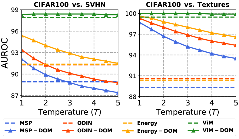
Figure 10: AUROC results of X-DOM using varying $\mathit{T}$ settings in the other two OOD dataset benchmark with CIFAR100 as the ID data.

B.2 Experiments on Large-scale Semantic Space

We implement X-DOM on the high-resolution large-scale dataset ImageNet-1k following the steps introduced in Sec. B.1 and evaluate its OOD detection performance in large-scale semantic spaces that have a large number of ID classes. There are two main differences in the implementation of large-scale experiments:

Stable Mask Generation for High-resolution Images We observe that since high-resolution images have richer appearance information, the network pays more attention to the most discriminative parts of the foreground object (e.g., the head of the fish). This leads to CAM assigning the highest class activation to the most discriminative parts and assigning the lower class activation to the rest part of the object, which degrades the quality of the resulting masks and does not completely segment the entire foreground object. Given that the average class activation of the whole object is still significantly higher than that of the background, we propose to use the mean value of the class activation of the whole image as the threshold for segmentation. As shown in Fig. 11, this trick significantly improves the pseudo-mask generated for high-resolution images.

High-resolution OOD Datasets In order to comprehensively evaluate the performance of X-DOM under high-resolution images, we add two high-resolution datasets as OOD datasets:

• ImageNet-O consists of images from classes that are not found in the ImageNet-1k dataset. It is adversarially filtered to fool the classifier and used to evaluate the robustness of the classifier to out-of-distribution data.

• SUN contains 130,519 high-definition scene images from 397 categories. Following [19], we select 50 nature-related categories that do not overlap with ImageNet-1k, and randomly sample 10,000 images as the OOD dataset.

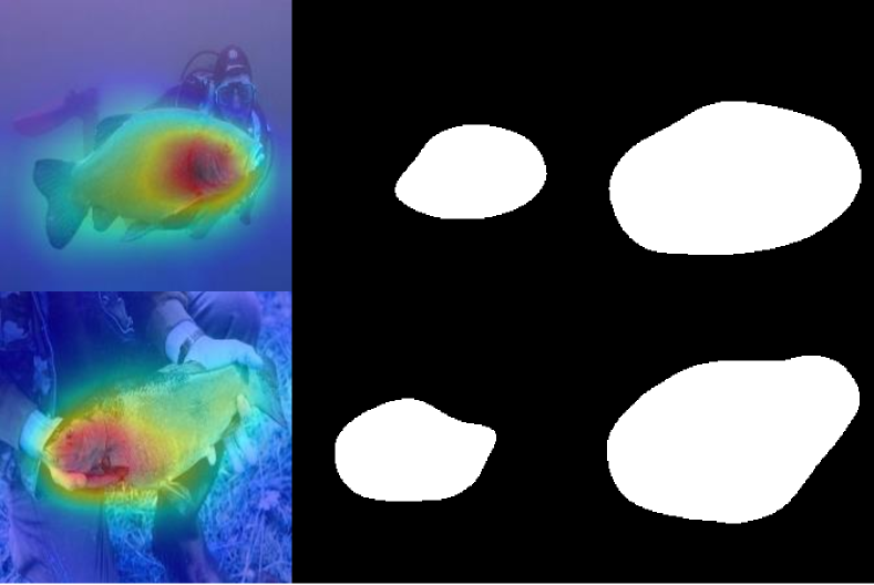
Figure 11: Examples of pseudo-masks generated for ImageNet1k using different strategies. (Left) CAM (Middle) Pseudo-masks generated using fixed threshold, and (Right) Pseudo-masks generated using mean class activation as the threshold.

Appendix C Additional Experiment Results

C.1 Detailed Analysis of OOD Scoring Methods

We report the detailed results of domain OOD scoring combined with all four post-hoc semantic OOD scoring methods in Tab. 5, including the use of domain OOD scores $S_{d}$ only (DOM), semantic OOD scores $S_{h}$ (Vanilla), and the full X-DOM model. Consistent with the results in the main text, using only the domain OOD scores in X-DOM can yield significantly improved performance on OOD benchmarks with significant domain differences from the in-distribution domain. Moreover, although DOM underperforms in the semantic-feature-dependent CIFAR100 vs. CIFAR10 benchmark, it still obtains competitive results in CIFAR10 vs. CIFAR100, which also relies on semantic features. This difference is caused by the number of ID categories, where more ID categories make the ID domain richer and more challenging to detect OOD samples by using domain features only. Holistically, the complete X-DOM achieves the best performance on most benchmarks, demonstrating the need to synthesize semantic and domain OOD scores.

C.2 Additional Results w.r.t. the Temperature Hyperparameter

Fig. 10 supplements the results of X-DOM on the remaining two benchmarks using various temperatures. Due to the SVHN, Textures and Places365 benchmarks having significant domain distribution differences, all methods’ performance gradually decreases as temperature increases. Note that stronger semantic OOD scoring methods (e.g., ViM) can significantly mitigate the decreasing performance trend. We choose $T=2.5$ as a trade-off between semantic and domain scores in our experiment.

Table 6: Comparison of X-DOM and outlier exposure (OE). ^† indicates that the results are taken from the original paper, and other methods share the same architecture. Reported results are averaged over the results on the four OOD datasets.

Methods	ID: CIFAR10		ID: CIFAR100
	FPR95$\downarrow$	AUROC$\uparrow$	FPR95$\downarrow$	AUROC$\uparrow$
Baseline	33.44	89.01	64.25	81.52
OE [15]	20.16	93.74	57.68	83.98
OE† [15]	15.57	96.40	52.30	83.47
X-DOM	7.87	98.04	42.29	91.03

C.3 X-DOM vs. Outlier Exposure

Domain features can also be alternatively learned by using the popular outlier exposure (OE) method [15] that uses external outlier data to support the learning. The comparison of X-DOM and OE is presented in Tab. 6, in which OE^† uses the large-scale 80M Tiny Image [35] as the outlier dataset, OE is trained using Tiny ImageNet [22] as the outlier data, OE, OE^† and X-DOM are all based on the MSP-based OOD scoring function, and Baseline is the original MSP without using outlier data. The results show that the two OE methods can also significantly outperform the Baseline model, but their performance is heavily dependent on the outlier data, e.g., the results of OE and OE^† differ significantly from each other. By contrast, X-DOM does not need outlier data and significantly outperforms both OE methods on both benchmarks.

References

- [1] Jiwoon Ahn, Sunghyun Cho, and Suha Kwak. Weakly supervised learning of instance segmentation with inter-pixel relations. In CVPR, pages 2209–2218, 2019.
- [2] Abhijit Bendale and Terrance E Boult. Towards open set deep networks. In CVPR, pages 1563–1572, 2016.
- [3] Jiefeng Chen, Yixuan Li, Xi Wu, Yingyu Liang, and Somesh Jha. Robust out-of-distribution detection via informative outlier mining. CoRR, abs/2006.15207, 2020.
- [4] Jiefeng Chen, Yixuan Li, Xi Wu, Yingyu Liang, and Somesh Jha. Robust out-of-distribution detection for neural networks. In The AAAI-22 Workshop on Adversarial Machine Learning and Beyond, 2021.
- [5] Mircea Cimpoi, Subhransu Maji, Iasonas Kokkinos, Sammy Mohamed, and Andrea Vedaldi. Describing textures in the wild. In CVPR, pages 3606–3613, 2014.
- [6] Matthew Cook, Alina Zare, and Paul D. Gader. Outlier detection through null space analysis of neural networks. CoRR, abs/2007.01263, 2020.
- [7] Jia Deng, Wei Dong, Richard Socher, Li-Jia Li, Kai Li, and Li Fei-Fei. Imagenet: A large-scale hierarchical image database. In CVPR, pages 248–255. Ieee, 2009.
- [8] Xin Dong, Junfeng Guo, Ang Li, Wei-Te Ting, Cong Liu, and HT Kung. Neural mean discrepancy for efficient out-of-distribution detection. In CVPR, pages 19217–19227, 2022.
- [9] Stanislav Fort, Jie Ren, and Balaji Lakshminarayanan. Exploring the limits of out-of-distribution detection. NeurIPS, 34:7068–7081, 2021.
- [10] Eduardo Dadalto Camara Gomes, Florence Alberge, Pierre Duhamel, and Pablo Piantanida. Igeood: An information geometry approach to out-of-distribution detection. In ICLR, 2022.
- [11] Matan Haroush, Tzviel Frostig, Ruth Heller, and Daniel Soudry. A statistical framework for efficient out of distribution detection in deep neural networks. In ICLR, 2022.
- [12] Kaiming He, Xiangyu Zhang, Shaoqing Ren, and Jian Sun. Identity mappings in deep residual networks. In ECCV, pages 630–645. Springer, 2016.
- [13] Dan Hendrycks, Steven Basart, Mantas Mazeika, Andy Zou, Joseph Kwon, Mohammadreza Mostajabi, Jacob Steinhardt, and Dawn Song. Scaling out-of-distribution detection for real-world settings. In ICML, pages 8759–8773, 2022.
- [14] Dan Hendrycks and Kevin Gimpel. A baseline for detecting misclassified and out-of-distribution examples in neural networks. ICLR, 2017.
- [15] Dan Hendrycks, Mantas Mazeika, and Thomas Dietterich. Deep anomaly detection with outlier exposure. In ICLR, 2019.
- [16] Dan Hendrycks, Kevin Zhao, Steven Basart, Jacob Steinhardt, and Dawn Song. Natural adversarial examples. In CVPR, pages 15262–15271, 2021.
- [17] Yen-Chang Hsu, Yilin Shen, Hongxia Jin, and Zsolt Kira. Generalized odin: Detecting out-of-distribution image without learning from out-of-distribution data. In CVPR, pages 10951–10960, 2020.
- [18] Rui Huang, Andrew Geng, and Yixuan Li. On the importance of gradients for detecting distributional shifts in the wild. NeurIPS, 34:677–689, 2021.
- [19] Rui Huang and Yixuan Li. Mos: Towards scaling out-of-distribution detection for large semantic space. In CVPR, pages 8710–8719, 2021.
- [20] Alexander Kolesnikov, Lucas Beyer, Xiaohua Zhai, Joan Puigcerver, Jessica Yung, Sylvain Gelly, and Neil Houlsby. Big transfer (bit): General visual representation learning. In ECCV, pages 491–507. Springer, 2020.
- [21] Alex Krizhevsky, Geoffrey Hinton, et al. Learning multiple layers of features from tiny images. 2009.
- [22] Ya Le and Xuan Yang. Tiny imagenet visual recognition challenge. CS 231N, 7(7):3, 2015.
- [23] Yann LeCun, Yoshua Bengio, and Geoffrey Hinton. Deep learning. nature, 521(7553):436–444, 2015.
- [24] Kimin Lee, Honglak Lee, Kibok Lee, and Jinwoo Shin. Training confidence-calibrated classifiers for detecting out-of-distribution samples. In ICLR, 2018.
- [25] Kimin Lee, Kibok Lee, Honglak Lee, and Jinwoo Shin. A simple unified framework for detecting out-of-distribution samples and adversarial attacks. NeurIPS, 31, 2018.
- [26] Shiyu Liang, Yixuan Li, and R. Srikant. Enhancing the reliability of out-of-distribution image detection in neural networks. In ICLR, 2018.
- [27] Weitang Liu, Xiaoyun Wang, John Owens, and Yixuan Li. Energy-based out-of-distribution detection. NeurIPS, 33:21464–21475, 2020.
- [28] Sina Mohseni, Mandar Pitale, JBS Yadawa, and Zhangyang Wang. Self-supervised learning for generalizable out-of-distribution detection. In AAAI, volume 34, pages 5216–5223, 2020.
- [29] Yuval Netzer, Tao Wang, Adam Coates, Alessandro Bissacco, Bo Wu, and Andrew Y Ng. Reading digits in natural images with unsupervised feature learning. 2011.
- [30] Aristotelis-Angelos Papadopoulos, Mohammad Reza Rajati, Nazim Shaikh, and Jiamian Wang. Outlier exposure with confidence control for out-of-distribution detection. Neurocomputing, 441:138–150, 2021.
- [31] Joaquin Quinonero-Candela, Masashi Sugiyama, Anton Schwaighofer, and Neil D Lawrence. Dataset shift in machine learning. Mit Press, 2008.
- [32] Jie Ren, Stanislav Fort, Jeremiah Liu, Abhijit Guha Roy, Shreyas Padhy, and Balaji Lakshminarayanan. A simple fix to mahalanobis distance for improving near-ood detection. ICML workshop on Uncertainty and Robustness in Deep Learning, 2021.
- [33] Chandramouli Shama Sastry and Sageev Oore. Detecting out-of-distribution examples with gram matrices. pages 8491–8501. PMLR, 2020.
- [34] Yiyou Sun, Chuan Guo, and Yixuan Li. React: Out-of-distribution detection with rectified activations. NeurIPS, 34:144–157, 2021.
- [35] Antonio Torralba, Rob Fergus, and William T Freeman. 80 million tiny images: A large data set for nonparametric object and scene recognition. IEEE TPAMI, 30(11):1958–1970, 2008.
- [36] Apoorv Vyas, Nataraj Jammalamadaka, Xia Zhu, Dipankar Das, Bharat Kaul, and Theodore L. Willke. Out-of-distribution detection using an ensemble of self supervised leave-out classifiers. In ECCV, September 2018.
- [37] Haoqi Wang, Zhizhong Li, Litong Feng, and Wayne Zhang. Vim: Out-of-distribution with virtual-logit matching. In CVPR, pages 4921–4930, 2022.
- [38] Haoran Wang, Weitang Liu, Alex Bocchieri, and Yixuan Li. Can multi-label classification networks know what they don’t know? NeurIPS, 34:29074–29087, 2021.
- [39] Jim Winkens, Rudy Bunel, Abhijit Guha Roy, Robert Stanforth, Vivek Natarajan, Joseph R. Ledsam, Patricia MacWilliams, Pushmeet Kohli, Alan Karthikesalingam, Simon Kohl, A. Taylan Cemgil, S. M. Ali Eslami, and Olaf Ronneberger. Contrastive training for improved out-of-distribution detection. CoRR, abs/2007.05566, 2020.
- [40] Zhi-Fan Wu, Tong Wei, Jianwen Jiang, Chaojie Mao, Mingqian Tang, and Yu-Feng Li. Ngc: A unified framework for learning with open-world noisy data. In ICCV, pages 62–71, October 2021.
- [41] Jianxiong Xiao, James Hays, Krista A Ehinger, Aude Oliva, and Antonio Torralba. Sun database: Large-scale scene recognition from abbey to zoo. In CVPR, pages 3485–3492. IEEE, 2010.
- [42] Jingkang Yang, Haoqi Wang, Litong Feng, Xiaopeng Yan, Huabin Zheng, Wayne Zhang, and Ziwei Liu. Semantically coherent out-of-distribution detection. In ICCV, pages 8301–8309, October 2021.
- [43] Alireza Zaeemzadeh, Niccolo Bisagno, Zeno Sambugaro, Nicola Conci, Nazanin Rahnavard, and Mubarak Shah. Out-of-distribution detection using union of 1-dimensional subspaces. In CVPR, pages 9452–9461, 2021.
- [44] Hongyi Zhang, Moustapha Cisse, Yann N. Dauphin, and David Lopez-Paz. mixup: Beyond empirical risk minimization. In ICLR, 2018.
- [45] Bolei Zhou, Aditya Khosla, Agata Lapedriza, Aude Oliva, and Antonio Torralba. Learning deep features for discriminative localization. In CVPR, pages 2921–2929, 2016.
- [46] Bolei Zhou, Agata Lapedriza, Aditya Khosla, Aude Oliva, and Antonio Torralba. Places: A 10 million image database for scene recognition. IEEE TPAMI, 40(6):1452–1464, 2017.
- [47] Ev Zisselman and Aviv Tamar. Deep residual flow for out of distribution detection. In CVPR, June 2020.