Thermal evolution of neutron stars in soft X-ray transients with thermodynamically consistent models of the accreted crust

Abstract

Thermal emission of neutron stars in soft X-ray transients (SXTs) in a quiescent state is believed to be powered by the heat deposited in the stellar crust due to nuclear reactions during accretion (deep crustal heating paradigm). Confronting observations of SXTs with simulations helps to verify theoretical models of the dense matter in the neutron stars. Usually, such simulations were carried out assuming that the free neutrons and nuclei in the inner crust move together. A recently proposed thermodynamically consistent approach allows for independent motion of the free neutrons. We simulate the thermal evolution of the SXTs within the thermodynamically consistent approach and compare the results with the traditional approach and with observations. For the latter, we consider a collection of quasi-equilibrium thermal luminosities of the SXTs in quiescence and the observed neutron star crust cooling in SXT MXB 1659$-$29. We test different models of the equation of state and baryon superfluidity and take into account additional heat sources in the shallow layers of neutron-star crust (the shallow heating). We find that the observed quasi-stationary thermal luminosities of the SXTs can be equally well fitted using the traditional and thermodynamically consistent models, provided that the shallow heat diffusion into the core is taken into account. The observed crust cooling in MXB 1659$-$29 can also be fitted in the frames of both models, but the choice of the model affects the derived parameters responsible for the thermal conductivity in the crust and for the shallow heating.

1 Introduction

Many neutron stars reside in binary systems with a lower-mass companion star (low-mass X-ray binaries, LMXBs) and accrete matter from the companion. Some of the LMXBs, called soft X-ray transients (SXTs), accrete intermittently, so that accretion episodes (outbursts) alternate with periods of quiescence. During an outburst, the emission is dominated by the accretion disk or a boundary layer (e.g., Inogamov & Sunyaev 2010; Gilfanov & Sunyaev 2014 and references therein). In quiescence, the accretion is switched off or strongly suppressed and the luminosity decreases by several orders of magnitude (see, e.g., Wijnands, Degenaar & Page 2017 for a review).

The accretion during an outburst leads to nuclear reactions in the crust accompanied by heat release. In particular, the heat is produced as the crust matter is pushed inside under the weight of newly accreted material, which is known as the deep crustal heating scenario (Sato, 1979; Haensel & Zdunik, 1990). Once an SXT turns to quiescence, the accumulated heat leaks through the surface. The so-called quasi-persistent SXTs have long outbursts (lasting months to years) that are sufficient to appreciably warm up their crust. During periods of quiescence between the outbursts, the thermal relaxation of the overheated crust can be observed through X-ray emission from the surface (e.g., Wijnands et al. 2017 and references therein).

An analysis of observations of the post-outburst cooling allows one to constrain the thermal conductivity and heat capacity of the crust (e.g., Rutledge et al. 2002; Shternin et al. 2007; Page & Reddy 2013). However, such an analysis can be complicated. Namely, the light curves of some SXTs in quiescence can be reproduced within the deep crustal heating scenario but require the so-called ‘shallow heating’ by some additional energy sources at relatively low densities (Brown & Cumming, 2009). Other SXTs may require some residual non-monotonic accretion during quiescence (e.g., Turlione, Aguilera & Pons 2015).

A traditional approach to calculation of the equation of state (EoS) and the heat release in the crust (Haensel & Zdunik, 1990, 2003, 2008; Fantina et al., 2018) is based on the assumption that free neutrons move together with the nuclei during accretion. Recently, the theoretical models of nuclear transformations during accretion, accreted crust composition and deep crustal heating have been revised by Gusakov & Chugunov (2020, 2021) and Shchechilin, Gusakov & Chugunov (2021, 2022), who found that free neutrons may redistribute independently of nuclei throughout the inner crust and core so as to satisfy the hydrostatic and diffusion equilibrium condition, $\mu_{n}^{\infty}={\rm constant}$, where $\mu_{n}^{\infty}$ is the chemical potential of free neutrons, redshifted to the reference frame of a distant observer. In the major part of the inner crust, where neutrons are superfluid, this condition is necessary for hydrostatic equilibrium of the system. The corresponding equilibration timescale is very short (of the order of the hydrodynamic timescale). In the rest of the inner crust, where neutrons are normal (in particular, in the small region near the outer-inner crust interface), this condition is necessary for the diffusion equilibrium of free neutrons. The associated timescale of reaching the equilibrium is also small (much smaller than the accretion timescale; Gusakov & Chugunov 2020).

As a result of implementing the hydrostatic/diffusion equilibrium condition, the EoS of the inner crust turns out to be closer to the EoS of the ground-state (‘catalysed’) matter, while the heat release inside the inner crust appears to be smaller than predicted by the traditional models. In this paper we examine the impact of these results on the thermal evolution of the SXTs and discuss some consequences for the analysis of the SXT observations.

The basic characteristics of the employed accreted crust models are outlined in Section 2. Section 3 is devoted to the modelling of the equilibrium thermal luminosities of the SXTs as functions of the mean accretion rates in the frames of the traditional and thermodynamically consistent models. We also pay attention to the effects of the shallow heating, the neutron star EoS and baryon superfluidity on these luminosities. In Section 4, we apply the different crust models to simulate the thermal evolution of a neutron star in an SXT during and after an outburst and compare the calculated light curves with observations, using SXT MXB 1659$-$29 as an example. Our conclusions are summarized in Section 5.

2 Accreted crust models

In the previous papers (Potekhin, Chugunov & Chabrier, 2019; Potekhin & Chabrier, 2021), we studied the thermal evolution of the SXTs for different EoSs, neutron-star masses $M$, nucleon superfluidity models and the total accretion time $t_{\mathrm{acc}}$, employing the theoretical models of the accreted crust (Haensel & Zdunik, 2008; Fantina et al., 2018), which followed the traditional paradigm, in which free (unbound) neutrons and nuclei move together in the inner crust. The results obtained with these two models proved to be similar, so in the present study we will limit ourselves to considering the more recent one (Fantina et al., 2018, hereafter F+18) as a representative of the traditional model.

The thermodynamically consistent accreted crust models, constructed by Gusakov & Chugunov (2020, 2021, hereafter GC), depend on the pressure $P_{\mathrm{oi}}$ at the interface between the outer and inner crust, where free neutrons appear. Because of their diffusion, $P_{\mathrm{oi}}$ may differ from the pressure at which neutrons start to drip out of nuclei. The value of $P_{\mathrm{oi}}$ is currently unknown, but the thermodynamic consistency and other arguments suggest that it should be between the minimum $P_{\mathrm{oi}}^{\mathrm{(0)}}$, which corresponds to the case where no heat is released in the inner crust (i.e., in the region with $P>P_{\mathrm{oi}}$), and maximum $P_{\mathrm{oi}}^{\mathrm{(cat)}}$, which roughly equals the neutron-drip pressure in cold catalysed matter. As in the traditional models, the crustal heating occurs at certain pressures (or in pressure intervals), where nuclear transformations take place. In the GC models, they occur at some values of $P<P_{\mathrm{oi}}$, at $P=P_{\mathrm{oi}}$, and at $P$ close to the bottom of the inner crust (where nuclei completely disintegrate into neutrons due to instability discussed in GC). The latter heat almost entirely leaks into the core because of the steep increase of thermal conductivity in the crust. The total heat produced in the outer and inner crust per each accreted baryon, $E_{\mathrm{h}}$, increases with an increase of $P_{\mathrm{oi}}$, while the heat produced at the outer-inner crust interface decreases (because the reactions there become less efficient at a larger electron Fermi momentum, corresponding to a larger $P_{\mathrm{oi}}$). The pressure values, at which the nuclear transformations occur, as well as the values of $P_{\mathrm{oi}}^{\mathrm{(0)}}$, $P_{\mathrm{oi}}^{\mathrm{(cat)}}$ and the amounts of heat released at each transformation, depend on the employed nuclear models. Gusakov & Chugunov (2021) presented these values for the finite-range droplet macroscopic model FRDM12 (Möller et al., 2016) and the family of models based on Hartree-Fock-Bogoliubov calculations with Skyrme-like effective nuclear forces BSk24, BSk25, BSk26 (Goriely, Chamel & Pearson, 2016).

Fig. 1 shows the total heat generated per accreted baryon, from the surface to a given density in the crust, as a function of mass density, for the F+18 model of the accreted crust and the GC models based on the BSk24 and BSk25 nuclear forces (which provide more plausible mass thresholds for rapid neutron-star cooling than BSk22 and BSk26, as argued by Pearson et al. 2018). We use the version of the F+18 model based on the BSk21 nuclear forces (Goriely, Chamel & Pearson, 2010) (table A.1 of Fantina et al. 2018). For the GC models, we consider the minimum and maximum values of $P_{\mathrm{oi}}$. The corresponding crust structure and heat production are presented in Tables 1 and 2. We assumed that the number fractions of protons $Y_{\mathrm{p}}=Z/A^{\prime}$ and free neutrons $Y_{\mathrm{nf}}=1-A/A^{\prime}$ among all nucleons equal the $Y_{\mathrm{p}}$ and $Y_{\mathrm{nf}}$ values in the non-accreted crust, fitted by Pearson et al. (2018). Here $Z$, $A$ and $A^{\prime}$ are the numbers of protons, bound nucleons and all nucleons in a Wigner-Seitz cell, respectively (they are needed to calculate the ion heat capacity and electron-ion transport coefficients). We also assume that the residual heat release in the deep layers of the inner crust, predicted by Gusakov & Chugunov (2021), occurs at the proton-drip point determined by Pearson et al. (2018).

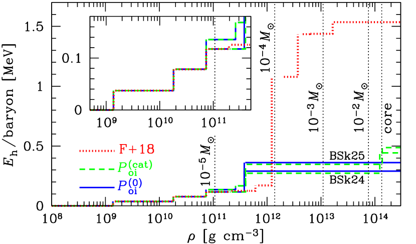
Figure 1: Total heat, $E_{\mathrm{h}}$, generated per accreted baryon in a layer from the star surface to a given density, as a function of mass density $\rho$, according to the model of Fantina et al. (2018) (F+18, dotted red line) and models of Gusakov & Chugunov (2021) with $P_{\mathrm{oi}}=P_{\mathrm{oi}}^{\mathrm{(cat)}}$ (dashed green lines) and $P_{\mathrm{oi}}=P_{\mathrm{oi}}^{\mathrm{(0)}}$ (solid blue lines), based on the models of nuclear interactions consistent with the EoSs BSk24 (lower lines) and BSk25 (upper lines). The gaps on the lines (best visible in the F+18 case) are due to the density jumps at the interfaces between neighbouring layers containing different nuclei. The right vertical dotted line corresponds to the crust-core transition according to the EoS BSk24; the other vertical dotted lines mark the $\rho$ values corresponding to four masses of overlying material, from $10^{-5}\,\mbox{M${}_{\odot}$}$ to $10^{-2}\,\mbox{M${}_{\odot}$}$, labelled near these lines, for a neutron star with gravitational mass $M=1.4\,\mbox{M${}_{\odot}$}$ and radius $R=12.6$ km. The inset shows a zoom-in of the low-density region.

Table 1: Nuclear composition and heat release in the accreted neutron-star crust according to the GC models (Gusakov & Chugunov, 2020, 2021) using the BSk24 nuclear mass table. The columns show the pressure $P$, at which a nuclear reaction occurs, the mass density $\rho$ before and after the reaction, the corresponding nuclear charge and mass numbers $Z$ and $A$ and the heat release per an accreted nucleon $\Delta E_{\mathrm{h}}$. The upper part of the table describes the outer crust and does not depend on $P_{\mathrm{oi}}^{\mathrm{(0)}}$, the middle part describes the interface at $P=P_{\mathrm{oi}}$ for $P_{\mathrm{oi}}=P_{\mathrm{oi}}^{\mathrm{(0)}}$ and the bottom part corresponds to the case of $P_{\mathrm{oi}}=P_{\mathrm{oi}}^{\mathrm{(cat)}}$. The last line shows the heat produced near the crust bottom; in this case we use the $\rho$ and $P$ values and the ratio $Z/A$ at the proton drip (not accompanied by a sharp nuclear transformation) according to Pearson et al. (2018).

$P$ [dyn cm-2]	$\rho$ [g cm-3]	$Z$	$A$	$\Delta E_{\mathrm{h}}$ [keV]
$6.46\times 10^{26}$	(1.37–1.48)$\times 10^{9}$	$26\to 24$	$56$	37
$1.83\times 10^{28}$	(1.81–1.97)$\times 10^{10}$	$24\to 22$	$56$	41
$1.06\times 10^{29}$	(7.36–8.08)$\times 10^{10}$	$22\to 20$	$56$	39
$3.36\times 10^{29}$	(1.93–2.03)$\times 10^{11}$	$20\to 19$	$56$	0
$3.50\times 10^{29}$	(2.09–2.20)$\times 10^{11}$	$19\to 18$	$56$	0
$P_{\mathrm{oi}}=P_{\mathrm{oi}}^{\mathrm{(0)}}$
$7.16\times 10^{29}$	(3.77–3.98)$\times 10^{11}$	$18\to 20$	$56\to 64$	$172$
$P_{\mathrm{oi}}=P_{\mathrm{oi}}^{\mathrm{(cat)}}$
$7.73\times 10^{29}$	(3.99–4.28)$\times 10^{11}$	$18\to 20$	$56\to 65$	$156$
$3.72\times 10^{32}$	$1.23\times 10^{14}$	$20$	$92$	$169$

Table 2: The same as in Table 1 but for the BSk25 nuclear masses.

$P$ [dyn cm-2]	$\rho$ [g cm-3]	$Z$	$A$	$\Delta E_{\mathrm{h}}$ [keV]
$6.46\times 10^{26}$	(1.37–1.48)$\times 10^{9}$	$26\to 24$	$56$	37
$1.83\times 10^{28}$	(1.81–1.97)$\times 10^{10}$	$24\to 22$	$56$	41
$1.06\times 10^{29}$	(7.36–8.08)$\times 10^{10}$	$22\to 20$	$56$	39
$5.00\times 10^{29}$	(2.59–2.88)$\times 10^{11}$	$20\to 18$	$56$	33
$P_{\mathrm{oi}}=P_{\mathrm{oi}}^{\mathrm{(0)}}$
$7.16\times 10^{29}$	(3.77–3.98)$\times 10^{11}$	$18\to 20$	$56\to 64$	$193$
$P_{\mathrm{oi}}=P_{\mathrm{oi}}^{\mathrm{(cat)}}$
$7.63\times 10^{29}$	(3.95–4.18)$\times 10^{11}$	$18\to 20$	$56\to 64$	$156$
$3.33\times 10^{32}$	$1.37\times 10^{14}$	$20$	$112$	$87$

The total heat release $E_{\mathrm{h}}$ in the entire accreted crust varies from 0.29 MeV for $P_{\mathrm{oi}}=P_{\mathrm{oi}}^{\mathrm{(0)}}$ to 0.44 MeV for $P_{\mathrm{oi}}=P_{\mathrm{oi}}^{\mathrm{(cat)}}$ in the BSk24 case (Table 1) and from 0.36 MeV for $P_{\mathrm{oi}}=P_{\mathrm{oi}}^{\mathrm{(0)}}$ to 0.49 MeV for $P_{\mathrm{oi}}=P_{\mathrm{oi}}^{\mathrm{(cat)}}$ in the BSk25 case (Table 2). These values are several times smaller than traditional ones: for example, $E_{\mathrm{h}}=1.54$ MeV in the F+18 case.

3 Equilibrium thermal emission

If the post-outburst thermal relaxation of the crust lasts sufficiently long time, the crust approaches thermal equilibrium with the core. Then the luminosity is a function of the core temperature, which is determined by the balance between energy income due to the accretion and the energy losses due to neutrino and photon emission. Since the time needed for an appreciable heating or cooling of the core is much longer than the accretion variability (Colpi et al., 2001), the equilibrium level is a function of the average mass accretion rate $\langle\dot{M}\rangle$. Here and hereafter, the angle brackets $\langle\ldots\rangle$ denote averaging over a time-span covering many outburst and quiescence cycles. The dependence of the equilibrium luminosity on $\langle\dot{M}\rangle$ is called heating curve (Yakovlev, Levenfish & Haensel, 2003).

Since the mass of a neutron-star crust is small ($\sim 10^{-2}\,\mbox{M${}_{\odot}$}$), the initial ground-state crust can be completely replaced by the reprocessed accreted material, if the accretion lasts long enough. The short spin periods of neutron stars in the SXTs ($<10$ ms for all but one SXTs with measured spin periods; see, e.g., table 2 in Potekhin et al. 2019 and references therein) can be explained by recycling due to the accretion of an appreciable mass. Therefore, in this paper we restrict ourselves to the fully accreted crust models.

We performed calculations of quiescent luminosities of neutron stars in the SXTs, similar to those presented in Potekhin et al. (2019), with essentially the same basic physics input. For the core EoS we consider the models BSk24, BSk25 (Pearson et al., 2018) and APR^∗ (Akmal et al. 1998, in the parametrized form of Potekhin & Chabrier 2018). The heat capacities, neutrino energy losses and thermal conductivities are treated essentially in the same way as described by Potekhin & Chabrier (2018), except for a small improvement for the electron thermal conductivities of outer envelopes composed of helium, described below. The employed models of baryon superfluidity are discussed in Section 3.3.

Fig. 2 shows the heating curves for neutron stars of different masses, based on the EoS model BSk24. The long-term average accretion rates $\langle\dot{M}\rangle$ and quasi-equilibrium bolometric thermal luminosities in quiescence $L_{\mathrm{q}}$ are plotted taking account of the gravitational redshift, as seen by a distant observer (thus corrected, they are denoted $\langle\dot{M}_{\mathrm{obs}}\rangle$ and $\tilde{L}_{\mathrm{q}}$; see Potekhin et al. 2019 for their calculation). The dashed heating curves are calculated using the GC crust models with the minimum and maximum values of the pressure $P_{\mathrm{oi}}$ at the outer-inner crust interface, as described in Section 2, while the dotted heating curves are computed according to the F+18 model. The curves of different colours correspond to neutron-star models with different masses. The error bars (arrows) represent the estimates of (upper limits to) $\langle\dot{M}_{\mathrm{obs}}\rangle$ and $\tilde{L}_{\mathrm{q}}$, derived from observations of the SXTs, as listed in Potekhin et al. (2019) but with updates for several objects: MXB 1659$-$29, HETE J1900.1$-$2455, Swift J1756.9$-$2508 and MAXI J0556$-$332. For MXB 1659$-$29 (object 7), an improved estimate of $\langle\dot{M}_{\mathrm{obs}}\rangle\sim 3\times 10^{-10}\,\mbox{M${}_{\odot}$}$ yr^-1 (Potekhin & Chabrier, 2021) is used. For HETE J1900.1$-$2455 (object 25), an updated estimate of $\tilde{L}_{\mathrm{q}}\approx\mbox{(1--2)}\times 10^{31}$ erg s^-1 follows from the results obtained by Degenaar et al. (2021) with atmospheric fits to the spectrum measured in 2018. Note that the crust of the neutron star in HETE J1900.1$-$2455 may not have yet reached thermal quasi-equilibrium by 2018 (Degenaar et al., 2021), therefore we consider this result as an upper limit. For Swift J1756.9$-$2508 (object 32), we updated the estimate of the average accretion rate, $\langle\dot{M}_{\mathrm{obs}}\rangle=5\times 10^{-12}\mbox{M${}_{\odot}$}\mbox{ yr}^{-1}$, according to Li et al. (2021).

For MAXI J0556$-$332 (object 35), we refined the data using the results recently published by Page et al. (2022). Four outbursts have been observed since its discovery in 2011, and the crust may not have reached thermal equilibrium between them. Therefore, just as in the case of HETE J1900.1$-$2455, the measured quiescent thermal luminosities can only be treated as upper limits to the quasi-equilibrium luminosity of MAXI J0556$-$332. The strongest upper limit $\tilde{L}_{\mathrm{q}}\lesssim 4\times 10^{33}$ erg s^-1 is provided by the results of the analysis of the XMM-Newton observation taken in 2019 (section 2.3 in Page et al. 2022); it refines the previous upper bound. We have also refined the estimate of $\langle\dot{M}_{\mathrm{obs}}\rangle$ for this source. Integrating $\dot{M}$ presented in the top panel of fig. 6 in Page et al. (2022) over time and dividing the result by the total time of observations, we obtain $\langle\dot{M}_{\mathrm{obs}}\rangle\approx 4.3\times 10^{-9}\,\mbox{M${}_{\odot}$}\mbox{~{}yr}^{-1}$.

The estimates of $\langle\dot{M}_{\mathrm{obs}}\rangle$ are rather uncertain, because the history of the SXTs observations (up to a few decades) is much shorter than the time of neutron star core heating due to accretion, which would be a proper interval for the time averaging. The estimate by Wijnands et al. (2013) for the latter time scale can be written as $\tau_{\mathrm{th}}\approx\mbox{(0.3--3)}\times 10^{4}\,L_{32}\,(\dot{M}_{-11}E_{\mathrm{h1}})^{-1}$ yr, where $L_{32}\equiv L_{\mathrm{q}}/(10^{32}$ erg s^-1), $\dot{M}_{-11}\equiv\langle\dot{M}\rangle/(10^{-11}\,\mbox{M${}_{\odot}$}\mbox{ yr}^{-1})$ and $E_{\mathrm{h1}}\equiv E_{\mathrm{h}}/1$ MeV. Therefore, the currently observed average accretion rate might be non-representative for some X-ray transients (see, e.g., Wijnands et al. 2013 for a discussion). In Fig. 2 we conditionally plot uncertainties of $\langle\dot{M}_{\mathrm{obs}}\rangle$ as a factor 2 around the most likely values based on the available observations (in the case of MXB 1659$-$29 this factor somewhat underestimates the true uncertainty – see Potekhin & Chabrier 2021).

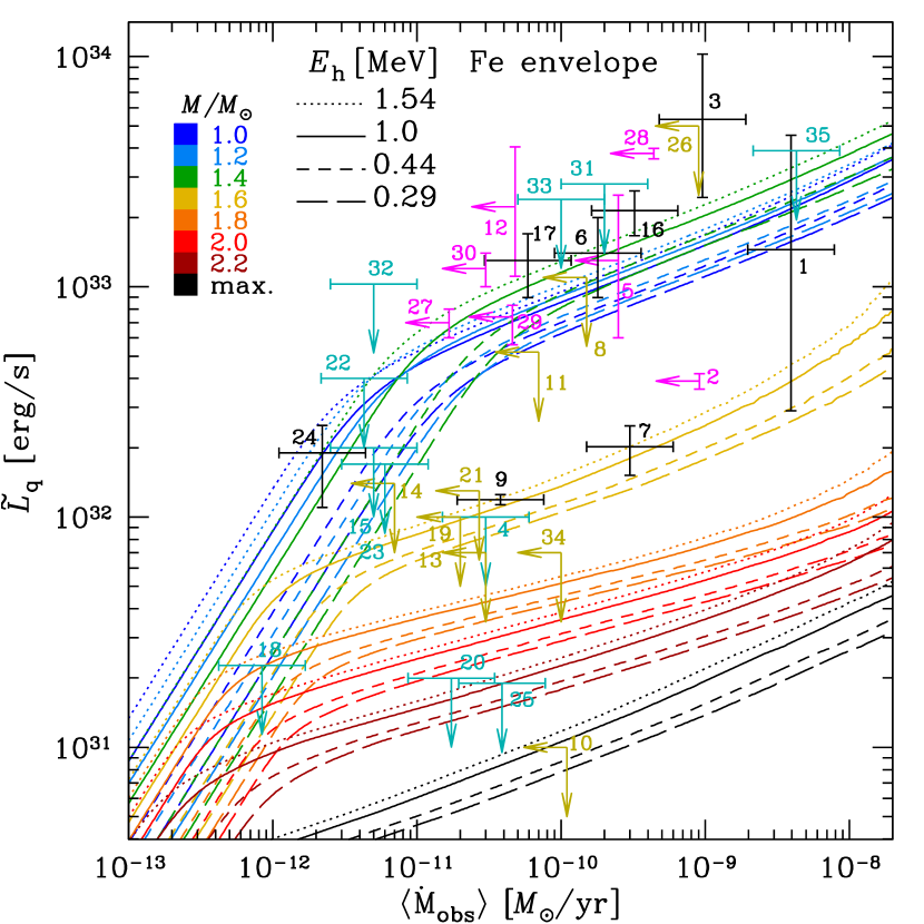
Figure 2: Quiescent thermal luminosities of SXTs as functions of average accretion rates in the reference frame of a distant observer. The iron heat-blanketing envelope is assumed. Solid errorbars and arrows show the data collected in Potekhin et al. (2019) for the observed SXTs coded with numbers: 4U 2129+47 (1), KS 1731$-$260 (2), 4U 1608$-$522 (3), EXO 1745$-$248 (4), 1M1716$-$315 (5), XTE 1709.5$-$267 (6), MXB 1659$-$29 (7), XB 1732$-$304 (8), Cen X-4 (9), 1H 1905+000 (10), SAX J1806.8$-$2435 (11), 4U 1730$-$22 (12), EXO 1747$-$214 (13), XTE 2123$-$058 (14), Aql X-1 (15), 4U1908+005 (16), SAX J1748.9$-$2021 (17), NGC 6440 X-2 (18), XTE J0929$-$314 (19), SAX J1808.4$-$3658 (20), XTE J1807$-$294 (21), XTE J1751$-$305 (22), XTE J1814$-$338 (23), IGR J00291+5934 (24), HETE J1900.1$-$2455 (25), XTE J1701$-$462 (26), IGR J17480$-$2446 (27), EXO 0748$-$676 (28), 1RXS J180408.9$-$342058 (29), Swift J174805.3$-$244637 (30), SAX J1750.8$-$2900 (31), Swift J1756.9$-$2508 (32), GRS 1747$-$312 (33), IGR J18245$-$2452 (34) and MAXI J0556$-$332 (35). The data for objects 7, 25, 32 and 35 have been updated, as explained in the text. The lines show theoretical predictions for neutron stars of different masses from $1.0\,\mbox{M${}_{\odot}$}$ to the maximum mass for the BSk24 EoS ($M_{\mathrm{max}}=2.28\,\mbox{M${}_{\odot}$}$), according to the colour map, computed for the heating power predicted either by the model F+18 (dotted lines) or by the thermodynamically consistent GC models with $P_{\mathrm{oi}}=P_{\mathrm{oi}}^{\mathrm{(0)}}$ (long-dashed lines) and $P_{\mathrm{oi}}=P_{\mathrm{oi}}^{\mathrm{(cat)}}$ (short-dashed lines). The solid lines correspond to the net neutron-star heating fixed at $E_{\mathrm{h}}=1.0$ MeV per accreted baryon.

Figure 3: The same as in Fig. 2, but with the heat-blanketing envelope composed of light elements (‘He envelope’, see text).

In Fig. 2, the outer crust of the star is assumed to be composed of the elements listed in Table 1 at all densities. In this case, the heat-blanketing envelope is made of iron within the ‘sensitivity strip’ (Gudmundsson, Pethick & Epstein, 1983) at $\rho\lesssim 10^{9}$ g cm^-3. Such a heat blanket is a relatively poor heat conductor. As the opposite extreme, in Fig. 3 we show the analogous heating curves calculated assuming that the heat blanket is made of the largest sustainable amount of helium, with carbon and oxygen beneath the helium layer. Such an envelope is most transparent to the heat transport (see Beznogov, Potekhin & Yakovlev, 2021, for a review); we call it the He envelope for short. We have taken account of the correction by Blouin et al. (2020) for the helium thermal conductivity at moderate electron degeneracy, modified according to Cassisi et al. (2021) (we used the modification version dubbed ‘B20sd’ by the latter authors). This update slightly affects the long-term cooling and heating curves of neutron stars with envelopes composed of light elements.

3.1 The long-term effect of shallow heating

From Figs. 2 and 3 we see that it is possible to reach a satisfactory agreement between the theory and observations for each SXT by varying the neutron star mass and envelope composition. However, for the hottest objects at the given accretion rates, such as IGR J00291+5934 (object 24), IGR J17480$-$2446 (object 27) or Swift J174805.3$-$244637 (object 30), the thermodynamically consistent GC models give somewhat larger discrepancies with observations than the F+18 model. This tension between the theory and observations can be alleviated by including the shallow heating, that is an additional heating at relatively low densities $\rho\sim 10^{8}-10^{10}$ g cm^-3, beside the predictions of the deep crustal heating theory. The shallow heating has been introduced into the theory by Brown & Cumming (2009) to match the slope between the first two observations of the SXT MXB 1659$-$29 after it had turned into the quiescent state. Later the shallow heating proved to be necessary to fit the theory with observations for most of the SXTs with observed crustal cooling in quiescence (see, e.g., results and discussions in Deibel et al. 2015; Waterhouse et al. 2016; Wijnands et al. 2017). Different theoretical fits to observed crust cooling curves in different SXTs require shallow heat deposit $E_{\mathrm{sh}}$ from 0 to several MeV per accreted nucleon, most typical values being $E_{\mathrm{sh}}\sim(0.2-2)$ MeV per nucleon (see Chamel et al. 2020 for a summary and references; see also Section 4 below).

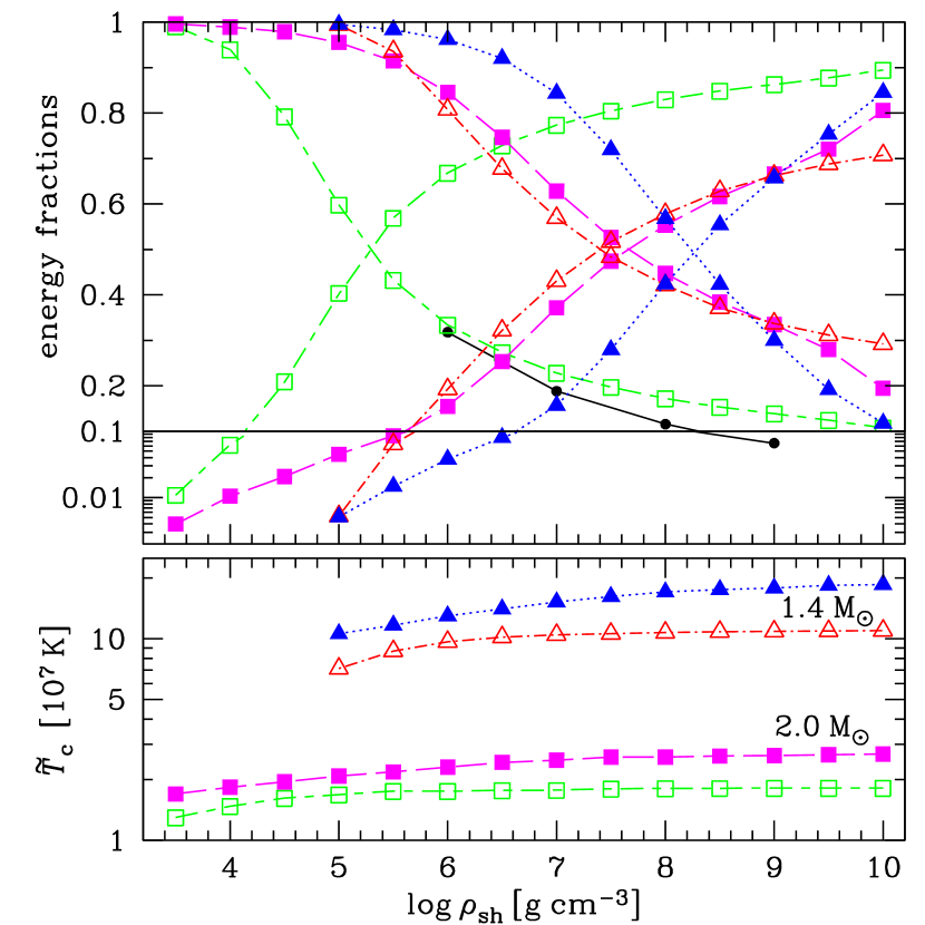
Figure 4: Top panel: The fractions of thermal energy deposited in a narrow layer close to a density $\rho_{\mathrm{sh}}$ leaking through the surface (decreasing dependences) and flowing into the core (increasing ones), computed assuming a stationary accretion. Triangles are for a neutron star with mass $M=1.4\,\mbox{M${}_{\odot}$}$ and radius $R=12.6$ km with the iron heat-blanketing envelope; squares are for a neutron star with $M=2.0\,\mbox{M${}_{\odot}$}$, $R=12.4$ km and the He envelope; empty symbols correspond to an accretion with $E_{\mathrm{sh}}\times\dot{M}=1\mbox{~{}MeV}\times 10^{-10}\,\mbox{M${}_{\odot}$}$ yr^-1 (then the total heating power is $H\approx 6\times 10^{33}$ erg s^-1 in the local reference frame); filled symbols correspond to a higher accretion rate $E_{\mathrm{sh}}\times\dot{M}=1\mbox{~{}MeV}\times 10^{-8}\,\mbox{M${}_{\odot}$}$ yr^-1 ($H\approx 6\times 10^{35}$ erg s^-1). The lines connecting the symbols serve as a guide for the eye. For comparison, the dots connected by the solid line show the fraction of energy from a short ($\sim 2$ minutes) superburst that is radiated from the atmosphere, according to the simulation results of Yakovlev et al. (2021). In the lower part of this panel, we use the logarithmic scale of the energy fraction to enhance visibility of its smallest values. Bottom panel: The stationary redshifted temperature in the core (in units of $10^{7}$ K) provided by the respective heating models shown using the same symbols and line styles as in the top panel.

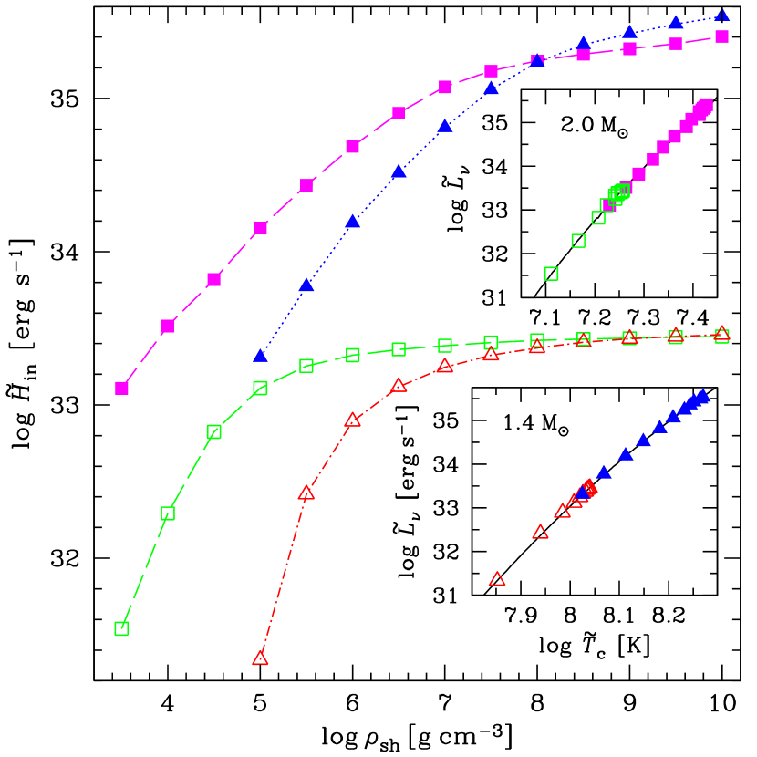
Figure 5: Logarithm of the redshifted heating power $\tilde{H}_{\mathrm{in}}$ injected into the core as function of $\rho_{\mathrm{sh}}$ for the same neutron star and heating models as in Fig. 4, plotted with the same symbols and line styles. The insets show logarithms of the total redshifted neutrino luminosity $\tilde{L}_{\nu}$ as a function of redshifted temperature in the core ($\tilde{L}_{\nu}=\tilde{H}_{\mathrm{in}}$ in the stationary state).

Ootes, Wijnands & Page (2019) noted that a large part of the shallow heat $E_{\mathrm{sh}}$ flows inside the star (we will denote this part $E_{\mathrm{sh}}^{\mathrm{in}}$ hereafter) and significantly contributes to the equilibrium state, resulting in an increase of the quiescent luminosity. Our calculations support this conclusion. To test it, we have numerically simulated thermal evolution of a neutron star assuming the shallow heating power concentrated at mass densities around $\rho_{\mathrm{sh}}$ in the narrow interval $\rho\in(0.95\rho_{\mathrm{sh}},1.05\rho_{\mathrm{sh}})$ according to the Wigner semicircle distribution. In the simulations we fixed $E_{\mathrm{sh}}=1$ MeV per an accreted nucleon and varied the accretion rate, the star mass and radius, and the envelope composition. Some results are presented in Figs. 4 and 5. The top panel in Fig. 4 shows the heating energy fractions that are either absorbed in the core or radiated from the surface as functions of the heating density $\rho_{\mathrm{sh}}$ for neutron-star models with $M=1.4\,\mbox{M${}_{\odot}$}$ and $M=2.0\,\mbox{M${}_{\odot}$}$, constructed according to the EoS BSk24, with the iron heat-blanketing envelope for the lighter star and the He envelope for the heavier star model. The energy fraction that eventually flows into the core, $E_{\mathrm{sh}}^{\mathrm{in}}/E_{\mathrm{sh}}$, depends on the model, but in any case we have $E_{\mathrm{sh}}^{\mathrm{in}}/E_{\mathrm{sh}}\gtrsim 1/2$ at $\rho_{\mathrm{sh}}\gtrsim 10^{8}$ g cm^-3. The bottom panel of Fig. 4 shows the temperature supported by the the stationary shallow heating (without other heating sources) in the deep layers of the inner crust and outer layers of the core. The inner temperatures are lower for the heavier neutron star model than for the lighter one because of the enhanced neutrino emission due to the direct Urca processes. Fig. 5 shows the $\rho_{\mathrm{sh}}$-dependence of the heating power supplied to the core, ${H}_{\mathrm{in}}=E_{\mathrm{sh}}^{\mathrm{in}}\dot{M}/m_{\mathrm{n}}$, where $m_{\mathrm{n}}$ is the nucleon mass. The insets illustrate the steep increase of the star’s neutrino luminosity with increasing temperature of the core, which explains the weakness of the temperature variation with changing $\rho_{\mathrm{sh}}$ in the bottom panel of Fig. 4. The plotted quantities are redshifted (i.e., reduced to the distant observer’s reference frame).

We have neglected the energy produced by the impact of accreted particles on the surface of the star. Some fraction of this energy propagates to the deeper layers and heats up the interior. The typical gravitational energy release of $\sim 200$ MeV per accreted baryon could provide an appreciable internal heating, if the fraction of the surface heat reaching the interior were $\gtrsim 10^{-3}$. However, $E_{\mathrm{sh}}^{\mathrm{in}}/E_{\mathrm{sh}}$ decreases so quickly as the heating location approaches the surface (cf. Fig. 4) that the required energy fraction $\gtrsim 10^{-3}$ seems unlikely.

The surface heating may also affect the outer boundary conditions for the heat diffusion problem through the dependence of thermal conductivity on temperature. This effect is hard to quantify, because the distribution of the surface heat under the spreading layer on the neutron star surface is poorly known, in particular because of its variability in time and space (see, e.g., Gilfanov & Sunyaev 2014 and references therein). Anyway, the model of stationary accretion that we employ in this section is only a crude approximation. Simulations of the short-term thermal response of a neutron star to a burst in the outer crust give qualitatively similar, but quantitatively different dependence of the heat fraction eventually radiated through the surface (the dots connected by solid lines in the top panel of Fig. 4, after Yakovlev et al. 2021).

Chamel et al. (2020) have shown that carbon or oxygen fusion, followed by electron captures in the crust of accreting neutron stars could provide up to $\approx 1.4$ MeV per an accreted nucleon (with the reservation that the actual energy release depends on the abundance of these elements). Then it would be plausible that up to $\sim 1$ MeV per accreted nucleon could be supplied to the core due to the shallow heating. For illustration, in Figs. 2 and 3 we plot the heating curves with $E_{\mathrm{h}}=1$ MeV, which corresponds to $E_{\mathrm{sh}}^{\mathrm{in}}$ equal to 0.71 MeV and 0.56 MeV in the cases where $P_{\mathrm{oi}}=P_{\mathrm{oi}}^{\mathrm{(0)}}$ and $P_{\mathrm{oi}}=P_{\mathrm{oi}}^{\mathrm{(cat)}}$, respectively.

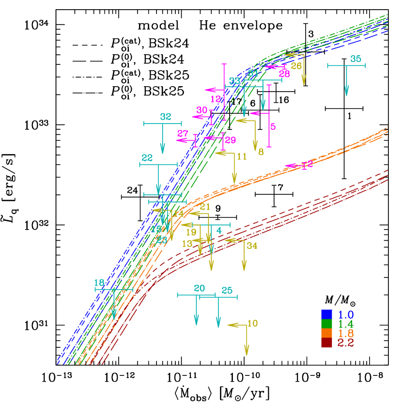
Figure 6: The observational points and heating curves from Fig. 3 for $M=1.0\,\mbox{M${}_{\odot}$}$, 1.4 M_⊙, 1.8 M_⊙ and 2.2 M_⊙ for the EoS BSk24 and the GC heating model according to Table 1 (long and short dashed lines for $P_{\mathrm{oi}}=P_{\mathrm{oi}}^{\mathrm{(0)}}$ and $P_{\mathrm{oi}}=P_{\mathrm{oi}}^{\mathrm{(cat)}}$) compared with the analogous heating curves for the EoS BSk25 and the heating power according to Table 2 (dot-long-dash and dot-short-dash lines for $P_{\mathrm{oi}}=P_{\mathrm{oi}}^{\mathrm{(0)}}$ and $P_{\mathrm{oi}}=P_{\mathrm{oi}}^{\mathrm{(cat)}}$, respectively).

3.2 The effects of the EoS choice

The EoS model BSk25 is somewhat stiffer than BSk24 and provides somewhat stronger deep crustal heating. We find that the use of the BSk25 model for the heating profile and crust composition (Table 2), as well as for the EoS, effective nucleon masses and composition of the core (Pearson et al., 2018) gives very similar results to the case of the BSk24 model. Fig. 6 presents a comparison of the heating curves obtained with these two models for the GC crust with the smallest and largest values of the parameter $P_{\mathrm{oi}}$.

The faintness of the coldest neutron stars in SXTs at quiescence, such as objects 4, 7, 9, 20, 25 in Figs. 2, 3, 6, can be explained by neutrino emission from their interiors due to powerful direct Urca processes. Such processes are only allowed at sufficiently large proton fraction $Y_{\mathrm{p}}$ ($Y_{\mathrm{p}}>1/9$ in the simplest case of the $npe$ matter – Haensel, 1995, see, e.g.,). This rules out the theoretical models that predict smaller $Y_{\mathrm{p}}$ at any densities relevant to the cores of neutron stars. Since $Y_{\mathrm{p}}$ usually increases with density in the core, the direct Urca processes are allowed at densities exceeding a certain threshold, $\rho>\rho_{\mathrm{DU}}$, which can be attained only in the central parts of neutron stars with masses above some threshold $M_{\mathrm{DU}}$. For the BSk24 and BSk25 models, $\rho_{\mathrm{DU}}=8.25\times 10^{14}$ g cm^-3 and $8.56\times 10^{14}$ g cm^-3, respectively. In both cases $M_{\mathrm{DU}}\approx 1.6\,\mbox{M${}_{\odot}$}$ (Pearson et al., 2018). For this reason, the relatively faint objects in Figs. 2, 3, 6 are matched by the heating curves for $M>1.6\,\mbox{M${}_{\odot}$}$.

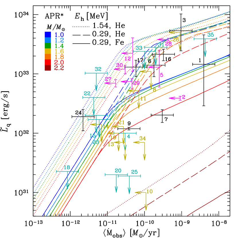
Figure 7: The observational points and heating curves for neutron stars of different masses and the GC model for $P_{\mathrm{oi}}=P_{\mathrm{oi}}^{\mathrm{(0)}}$ with the He envelope (long-dashed lines) and heavy-element (Fe) envelope (solid curves), as in Figs. 2 and 3, but computed using the APR^∗ model for the EoS and composition of the core.

Fig. 7 demonstrates the heating curves computed using the widely used EoS model APR^∗ (Akmal, Pandharipande & Ravenhall, 1998) in the neutron star core (as parametrized by Potekhin & Chabrier 2018) and the BSk24 model in the crust. In this case, $\rho_{\mathrm{DU}}=1.56\times 10^{15}$ g cm^-3 and $M_{\mathrm{DU}}=2.006\,\mbox{M${}_{\odot}$}$, which necessitates fine tuning of the mass around $M\approx 2\,\mbox{M${}_{\odot}$}$ to match the heating curves of some relatively faint SXTs with the observations. However, still much finer tuning would be needed, if we neglected the enhancement of the modified Urca processes (which are the main neutrino emission processes at $\rho<\rho_{\mathrm{DU}}$) at $\rho\sim\rho_{\mathrm{DU}}$, discovered by Shternin et al. (2018). This enhancement becomes very strong at $\rho\approx\rho_{\mathrm{DU}}$, which may be qualitatively regarded as ‘smearing’ the direct Urca threshold. For the APR^∗ model, this effect noticeably enhances the total neutrino luminosity of the neutron stars with $M\approx(1.8-2.0)\,\mbox{M${}_{\odot}$}$ and thus decreases their temperatures. In the absence of such enhancement, the heating curves of all neutron stars with $M\leq 2\,\mbox{M${}_{\odot}$}$ in Fig. 7 would be close to each other.

3.3 The effects of baryon superfluidity

The thermal evolution of neutron stars can be affected by baryon superfluidity (see, e.g., Page et al. 2014; Sedrakian & Clark 2019, for review and references). The three principal types of the superfluidity arise from neutron singlet (ns), proton singlet (ps) and neutron triplet (nt) types of Cooper pairing. The effects of each superfluidity type are conveniently parametrized by the dependence of the corresponding critical temperature $T_{\mathrm{crit}}$ on the mean baryon number density $n_{\mathrm{b}}$ or the mass density $\rho$ (see, e.g., Yakovlev et al. 2001, for review and references). In Figs. 2–6 we used the parametrizations MSH, BS and TTav by Ho et al. (2015) to the microscopic calculations by Margueron, Sagawa & Hagino (2008); Baldo & Schulze (2007); Takatsuka & Tamagaki (2004) for the ns, ps and nt pairing types, respectively. The corresponding density dependences of $T_{\mathrm{crit}}$ are shown in Fig. 8.

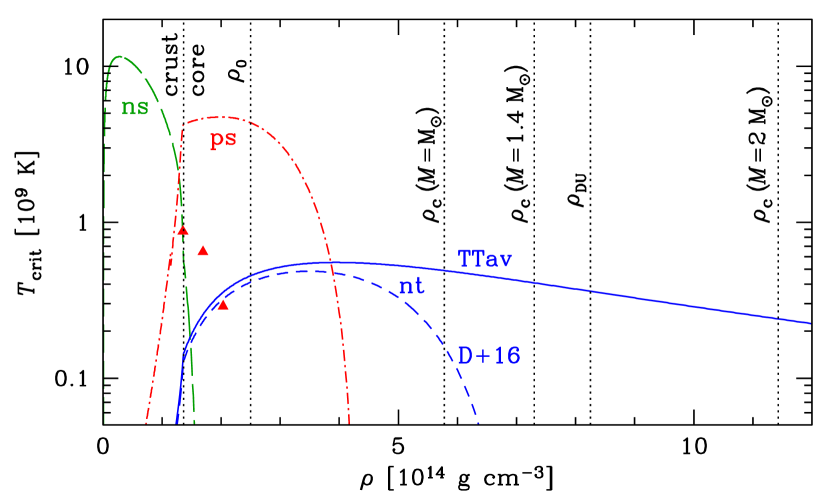
Figure 8: Critical temperature for nucleon superfluidity as a function of mass density for neutron singlet (ns), proton singlet (ps) and neutron triplet (nt) pairing. The long-dashed, dot-dash and solid lines correspond to the superfluid gap parametrizations by Ho et al. (2015) named MSH, BS and TTav for theoretical calculations by Margueron et al. (2008) for the ns pairing, Baldo & Schulze (2007) for the ps pairing and Takatsuka & Tamagaki (2004) for the nt pairing, respectively. The short-dashed line shows the parametrization by Ding et al. (2016) to their calculations for the nt pairing, and the triangles show the results of Guo et al. (2019) for the ps pairing. The vertical dotted lines are drawn at the densities corresponding to the crust-core boundary, nuclear saturation density $\rho_{0}$ (Horowitz, Piekarewicz & Reed, 2020), direct Urca threshold $\rho_{\mathrm{DU}}$ and densities $\rho_{\mathrm{c}}$ at the centre of neutron stars with masses $M=1\,\mbox{M${}_{\odot}$}$, $1.4\,\mbox{M${}_{\odot}$}$ and $2.0\,\mbox{M${}_{\odot}$}$, according to the EoS BSk24 (Pearson et al., 2018).

Margueron et al. (2008) and Gandolfi et al. (2009) reported similar theoretical dependences of $T_{\mathrm{crit}}$ on baryon density for the ns-type pairing. Previously we have checked that the replacement of one of these models by the other does not appreciably change the thermal evolution of the isolated neutron stars (Potekhin & Chabrier, 2018) and the accreting neutron stars in the SXTs (Potekhin et al., 2019; Potekhin & Chabrier, 2021). Results of recent numerical simulations of the neutron singlet superfluidity by Ding et al. (2016) are also close to the MSH model.

Baldo & Schulze (2007) showed that the allowance for the three-body effective nuclear forces and for in-medium effects (such as modified effective nucleon masses and polarization) reduces the gap in the proton energy spectrum caused by the ps-pairing, $\Delta_{\mathrm{ps}}$, which is related to the critical temperature of superfluidity, $\mbox{$k_{\mathrm{B}}$}T_{\mathrm{crit}}=0.5669\,\Delta_{\mathrm{ps}}$. Guo et al. (2019) have argued that a proper account of the density dependence of the proton-proton induced interaction in the neutron star matter leads to still stronger suppression of the ps-type superfluidity. The values of $T_{\mathrm{crit}}$ that follows from their tabular values of $\Delta_{\mathrm{ps}}$ are shown in Fig. 8 by the triangles. Lim & Holt (2021) have recently studied proton pairing in neutron stars using the chiral effective field theory and obtained a broad variety of gaps as functions of the proton Fermi momentum $k_{\mathrm{F}}^{\mathrm{p}}$, depending on the details of the theoretical model. All these gaps are either similar to or smaller than the BS gap. Sedrakian & Clark (2019) suggested that the absence of proton superconductivity may have profound implications for the physics of compact stars. We tested the effect of the reduction of the ps-type critical temperature by using the extreme model of completely suppressed proton superfluidity and found that it almost does not affect the heating curves shown in Figs. 2, 3, 6. This is explained by the fact that the non-suppressed BS proton pairing gap vanishes at the centres of all neutron stars with $M>\mbox{M${}_{\odot}$}$, hence a substantial part of the core is free of the proton superfluidity in all considered models.

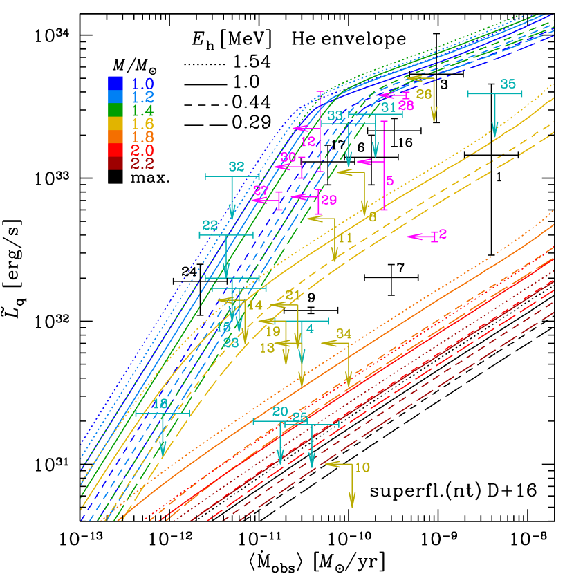
Figure 9: The same as in Fig. 3, but with another model of the neutron triplet-type superfluidity (D+16 instead of TTav).

However, the current uncertainties in the theory of the triplet pairing of baryons prove to be essential for the simulations of the thermal evolution of neutron stars (see, e.g., Fortin et al. 2018; Potekhin et al. 2019, 2020; Burgio et al. 2021 and references therein). The main effect of the superfluidity in the core on the quasi-stationary states and long-term evolution of the neutron stars consists in suppressing the direct Urca processes. Due to this effect, the decrease of the luminosity with increasing mass above $M_{\mathrm{DU}}$ is less sharp than it would be in the absence of superfluidity. As an example alternative to the TTav model, the short-dashed line in Fig. 8 represents the parametrization of Ding et al. (2016) to their numerical results, based on the same Av18 effective nucleon-nucleon potential as implied in the TTav model, with short- and long-range neutron correlations included (hereafter, D+16). Fig. 8 reveals that the TTav and D+16 models predict similar $T_{\mathrm{crit}}(\rho)$ dependences at relatively small $\rho$ up to the maximum $T_{\mathrm{crit}}^{\mathrm{(max)}}\approx(5-7)\times 10^{8}$ K at $\rho\approx 4\times 10^{14}$ g cm^-3, but at higher densities the D+16 superfluidity becomes quickly suppressed, unlike the TTav one. The D+16 parametrization is used in Fig. 9, which should be compared with Fig. 3, where we employed the TTav model using the same models of the EoS and the heat-blanketing envelope. Because of vanishing D+16 superfluidity at $\rho\gtrsim 7\times 10^{14}$ g cm^-3, any neutron star with $M>M_{\mathrm{DU}}$ has some central region where the direct Urca process is not suppressed by superfluidity. This causes a sharper lowering of the heating curves (i.e., decrease of $\tilde{L}_{\mathrm{q}}$ with increasing $M$ at a given $\langle\dot{M}_{\mathrm{obs}}\rangle$) in Fig. 9 relative to Fig. 3 for $M>M_{\mathrm{DU}}$.

Let us note that the parametrization by Ding et al. (2016) is based on their computations without inclusion of three-nucleon forces (3NF). The preliminary results with inclusion of the 3NF effects, presented by these authors, show an increase of the triplet gap (in contrast with the singlet pairing case) and do not demonstrate the gap closure at large densities, so that the TTav gap appears to be between the results of Ding et al. (2016) with and without the 3NF. The authors caution that at these high densities one approaches the limit of applicability of the employed theory.

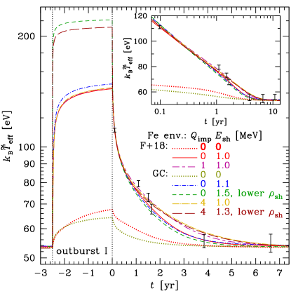
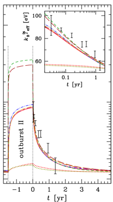
Figure 10: Simulated light curves for the outbursts I (left panel) and II (right panel) of MXB 1659$-$29 versus observations. The shown dependences of the effective temperature in energy units, $\mbox{$k_{\mathrm{B}}$}\tilde{T}_{\mathrm{eff}}$, on time $t$, as measured by a distant observer from the end of an outburst, have been computed using the BSk24 EoS model for a neutron star with $M=1.6\,\mbox{M${}_{\odot}$}$ with an iron outer envelope under different assumptions about the accreted crust. The upper dotted curve, solid curve and long-dash—short-dash curve are calculated assuming the F+18 model, and the other curves illustrate the case of the GC model with $P_{\mathrm{oi}}=P_{\mathrm{oi}}^{\mathrm{(0)}}$. The dotted lines show the case of no shallow heating and the other lines include the amount of heat per accreted nucleon $E_{\mathrm{sh}}$ as quoted in the legend. The mass density of the shallow heating is taken to be $\rho_{\mathrm{sh}}=1.4\times 10^{9}$ g cm^-3 for all the curves except the ones marked ‘lower $\rho_{\mathrm{sh}}$’ in the legend: for these two curves $\rho_{\mathrm{sh}}=10^{8}$ g cm^-3. The impurity parameter $Q_{\mathrm{imp}}$ is also listed in the legend for each case. The rising parts of the curves at $t<0$ show the increase of conditional effective temperature during an outburst, calculated neglecting the accretion-induced processes near the surface. The error bars represent the values derived from observations, according to Parikh et al. (2019). The insets show the crust cooling curves plotted at a logarithmic time scale.

4 Crust cooling: the case of MXB 1659–29

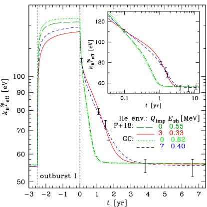
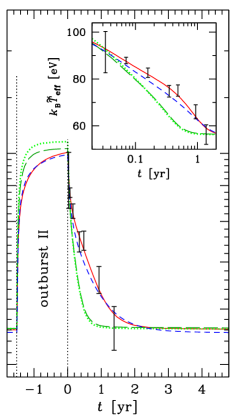
Figure 11: The simulated light curves and observational error bars, analogous to Fig. 10, but for a neutron star of mass $M=1.8\,\mbox{M${}_{\odot}$}$ with the helium atmosphere and ocean down to the interface with the accreted crust at mass density $\rho=10^{8}$ g cm^-3. The curves of different styles correspond to different $Q_{\mathrm{imp}}$ and $E_{\mathrm{sh}}$ in the crust, according to the legend.

Let us apply the accreted crust models described in Section 2 to a study of the thermal evolution of the SXT MXB 1659$-$29 (MAXI J1702$-$301). We have chosen this quasi-persistent transient as an example, because it has been observed for a long time, revealed three outbursts and has a well documented record of the crust cooling after the last two of them. It was discovered as an X-ray bursting source during the SAS-3 satellite mission (Lewin et al., 1976; Lewin & Joss, 1977). Later it was observed many times using different instruments (see Wijnands et al. 2003; Parikh et al. 2019 and references therein). The source was detected several times in X-rays and in the optical from October 1, 1976 till July 2, 1979, but then (between July 2 and July 17, 1979; Cominsky, Ossmann & Lewin 1983) it turned to quiescence and could not be detected any more until April 1999, when in ’t Zand et al. (1999) found it to be active again. The source remained bright for almost 2.5 years before it became dormant in September 2001. It was first observed in the quiescent state by Chandra in October 2001 (Wijnands et al., 2003). Afterwards, its X-ray emission was observed several times in quiescence till October 2012 (Cackett et al., 2006, 2008, 2013). In August 2015 the source showed a new outburst (Negoro et al., 2015), which lasted $\approx 550$ days till February 2017. Subsequent crust cooling was followed from March 2017 using X-ray observatories Swift, Chandra and XMM-Newton. The results have been summarized and analyzed by Parikh et al. (2019). Following these authors, we name outburst I and outburst II those of 1999–2001 (MJD 51265–52162) and 2015–2017 (MJD 57256–57809.7), respectively; we also name outburst 0 the one observed in 1976–1979. The quiescent light curves after the end of outburst I were modeled in a number of works (Brown & Cumming, 2009; Cackett et al., 2013; Deibel et al., 2017; Parikh et al., 2019; Potekhin & Chabrier, 2021; Mendes et al., 2022). Parikh et al. (2019) and Potekhin & Chabrier (2021) performed consistent modelling of the short-term evolution of MXB 1659$-$29 during and after the two outbursts I and II. In all the cases, additional adjustable model parameters were necessary for good fits: the heat deposited at shallow depths per accreted baryon, $E_{\mathrm{sh}}$, and the mean-square deviation of the nuclear charge number due to impurities in the crust, $Q_{\mathrm{imp}}$. The latter parameter modifies the electron thermal conductivity of the crust: the larger $Q_{\mathrm{imp}}$, the smaller the conductivity.

The previous studies were based on the traditional models of the nuclear transformations and heat production in the accreted crust. Here we use the case of MXB 1659$-$29 to illustrate the influence of neutron redistribution in the inner crust on the post-outburst cooling of neutron stars in SXTs. For this purpose we will compare the results of numerical simulations of the thermal evolution of the neutron star in this SXT, performed using the traditional (F+18) and thermodynamically consistent (GC) accreted crust models. For each model, we first prepare a quasi-equilibrium thermal state of a neutron star so as to match the most probable value of the redshifted effective temperature $\tilde{T}_{\mathrm{eff}}$ in quiescence, derived from observations, $\mbox{$k_{\mathrm{B}}$}\tilde{T}_{\mathrm{eff}}\approx 56$ eV (Cackett et al., 2008, 2013). Then we consecutively simulate the neutron star heating during outburst 0, followed by cooling during 20 years, heating during outburst I, followed by cooling during 13.9 years and heating during outburst II, followed by cooling till now. In the absence of detailed information on the early outburst 0, we assume that it has the same characteristics as outburst I. We fix $\dot{M}=4\times 10^{-9}\,\mbox{M${}_{\odot}$}$ yr^-1 for the outburst I and $\dot{M}=1.3\times 10^{-9}\,\mbox{M${}_{\odot}$}$ yr^-1 for outburst II (see Potekhin & Chabrier, 2021, for details).

First let us consider the heavy-element (Fe) heat-blanketing envelope model. In this case, as can be seen from Figs. 2 and 7, it can be compatible with the estimated $\langle\dot{M}\rangle$ and $\tilde{L}_{\mathrm{q}}$ only if $M\approx M_{\mathrm{DU}}$. For illustration we assume the BSk24 EoS and accordingly fix $M=1.6\,\mbox{M${}_{\odot}$}$. The results are shown in Fig. 10. The upper and lower dotted lines correspond to the F+18 and GC models, respectively, without any adjustable ingredients, i.e., with $E_{\mathrm{sh}}=0$ and $Q_{\mathrm{imp}}=0$. We see that they cannot reproduce the amplitude of the observed crust cooling. The other light curves in this figure are calculated by adjusting $E_{\mathrm{sh}}$ so as to match the first measurement of $\tilde{T}_{\mathrm{eff}}$ after the end of outburst I (the Chandra observation on October 15, 2001, about one month after the source became quiescent). We find that we need to include $E_{\mathrm{sh}}\approx 1$ MeV, if it is located near the shallowest nuclear transformation in the F+18 and GC models of accreted crust, $\rho_{\mathrm{sh}}\approx 1.4\times 10^{9}$ g cm^-3 (that is near the inner boundary of the region where burning of light elements to iron can be compatible with the data in Tables 1 and 2), which is our default value. If the shallow heating occurs at a smaller density, then the heat amount $E_{\mathrm{sh}}$ should be somewhat larger, because its larger part leaks to the surface and does not heat the inner layers (cf. Fig. 4). For example, the dashed curves in Fig. 10 illustrate the case where $\rho_{\mathrm{sh}}=10^{8}$ g cm^-3. A comparison with the case of the default shallow depth (the dot-dashed curve) shows that the crust cooling is rather insensitive to the shallow heating depth at $t\gtrsim 0.1$ yr, but the smaller $\rho_{\mathrm{sh}}$ gives a better agreement with the observations of outburst II at $t\lesssim 0.1$ yr (see the inset in the right panel of Fig. 10).

An admixture of charge impurities helps us to achieve a better agreement between the theoretical crust cooling curves and observations. For simplicity, we assume constant impurity level $Q_{\mathrm{imp}}$ in the entire solid crust. The optimal values are $Q_{\mathrm{imp}}\approx 1$ and $Q_{\mathrm{imp}}\approx 4$ in the F+18 and GC models, respectively.

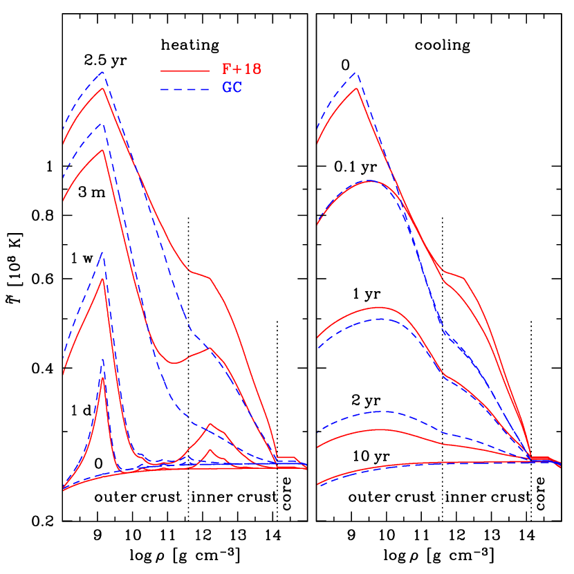
Figure 12: Redshifted temperature profiles inside a neutron star as in Fig. 11 during the outburst I (left panel) and subsequent cooling (right panel) at different times after the start of the heating and the cooling, respectively, as marked near the curves. The same neutron star model as in Fig. 11 is used. The solid and dashed curves represent the results for the accreted crust models F+18 and GC with the same accretion rate, shallow heating and impurity parameters as for the respective curves in the left panel of Fig. 11. The vertical dotted lines indicate the outer-inner catalyzed crust and crust-core interfaces.

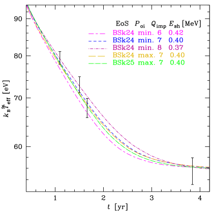
Figure 13: Comparison of the best-fit simulated light curve for the GC model from Fig. 11, left panel (the blue short-dashed line) with light curves computed, as clarified in the legend, for different $Q_{\mathrm{imp}}$ and $E_{\mathrm{sh}}$ in the crust and for the model with $P_{\mathrm{oi}}=P_{\mathrm{oi}}^{\mathrm{(cat)}}$ (marked ‘max.’ in the legend, whereas the choice $P_{\mathrm{oi}}=P_{\mathrm{oi}}^{\mathrm{(0)}}$ is marked ‘min.’), for the models BSk24 and BSk25.

Let us consider another model of the heat-blanketing envelope, which is composed of He at $\rho<10^{8}$ g cm^-3 and is consistent with the adopted accreted crust model (either GC or F+18) at $\rho>10^{8}$ g cm^-3. This envelope is slightly less heat-transparent than the He envelope considered in Section 3. Keeping the BSk24 EoS in the core, we find that the realistic mean accretion rates $\langle\dot{M}_{\mathrm{obs}}\rangle\sim 10^{-10}-10^{-9}\,\mbox{M${}_{\odot}$}$ yr^-1 are compatible with the estimated surface temperature in quiescence, $\tilde{T}_{\mathrm{eff}}=56\pm 2$ eV (Cackett et al., 2013; Parikh et al., 2019), if $M\approx(1.7-2.0)\,\mbox{M${}_{\odot}$}$, depending on the nt-superfluidity model ($\approx 2.0\,\mbox{M${}_{\odot}$}$ for the TTav model and $\approx 1.7\,\mbox{M${}_{\odot}$}$ for the D+16 model; cf. Figs. 3 and 9). The results of the simulations with fixed $M=1.8\,\mbox{M${}_{\odot}$}$ are shown in Fig. 11. Here, all light curves are calculated with $E_{\mathrm{sh}}$ adjusted so as to match the first measurement of $\tilde{T}_{\mathrm{eff}}$ after the end of outburst I. Assuming $Q_{\mathrm{imp}}=0$, we obtain very similar light curves for the F+18 and GC models,which exhibit a fast post-outburst cooling incompatible with the observations. We see that an acceptable agreement between the theory and observations can be achieved if we assume $Q_{\mathrm{imp}}\approx 3$ in the F+18 model or $Q_{\mathrm{imp}}\approx 7$ in the GC model. It is remarkable that the observations of both outbursts I and II can be fitted by using the same values of $E_{\mathrm{sh}}$ and $Q_{\mathrm{imp}}$.

The presented results demonstrate that the F+18 model provides somewhat better agreement with the observations than the GC model, although this difference is statistically insignificant. It is due to the retarded cooling in the F+18 model at intermediate times $t\sim(0.1-1)$ yr, which is absent in the GC model. Fig. 12 provides an insight into the origin of this retardation. In the traditional model, unlike the GC model, the inner crust layers at $\rho\sim 10^{12}-10^{13}$ g cm^-3 are heated appreciably during the outburst. This inner-crust heat does not affect the initial cooling stage, as we see from the near constancy of $\tilde{T}$ at densities of a few times $10^{11}$ g cm^-3 at $t\lesssim 0.1$ yr. At $t\gtrsim 0.1$ yr, however, this additional heat propagates to the surface and is radiated, making the luminosity somewhat higher than in the GC model. In the right panel of Fig. 12, the temperature profiles at $\rho\lesssim 10^{9}$ g cm^-3 are lower in the F+18 model than in the GC model at early times $t<0.1$ yr because of the stronger preceding shallow heating, but become higher at $t\sim 1$ yr due to the heat income from the inner crust. At $t\gtrsim 2$ yr the GC profiles become higher again because the heat dissipates less quickly due to the larger impurity parameter (i.e., lower conductivity of the crust).

Fig. 13 illustrates theoretical variations of the SXT crust cooling behaviour in frames of the GC models. First, we vary $Q_{\mathrm{imp}}$ around the best-fit GC model shown in Fig. 11 and adjust $E_{\mathrm{sh}}$ as previously. We see that the observational error bars allow variation of $Q_{\mathrm{imp}}$ by $\sim 20$%, an increase of $Q_{\mathrm{imp}}$ being accompanied by a decrease of $E_{\mathrm{sh}}$. Next, we test the model with the largest $P_{\mathrm{oi}}$ value ($P_{\mathrm{oi}}=P_{\mathrm{oi}}^{\mathrm{(cat)}}$), instead of the smallest one ($P_{\mathrm{oi}}=P_{\mathrm{oi}}^{\mathrm{(0)}}$). Finally, we replace the BSk24 model for the heating profile and crust composition (Table 1) by the BSk25 model (Table 2). As we see, neither the variation of $P_{\mathrm{oi}}$ nor the replacement of BSk24 by BSk25 can affect the crust cooling appreciably. This is explained by the dominant influence of the heat sources in the outer crust (including the shallow heating), which are the same in these models.

5 Conclusions

We studied the consequences of hydrostatic/diffusion equilibrium of free neutrons in accreted inner crust on the long- and short-term thermal evolution of the neutron stars in the SXTs. We found that the observed quasi-stationary thermal luminosities of such neutron stars can be equally well fitted in the frames of the model F+18 (Fantina et al., 2018), based on the traditional approach that neglects the hydrostatic/diffusion equilibrium condition for free neutrons and the models GC (Gusakov & Chugunov, 2020, 2021), which take this condition into account. However, in the latter model, unlike the traditional ones, good fits of some relatively hot quiescent sources can only be obtained provided that the heating of the neutron star core by the energy sources located at shallow depths in the outer crust is allowed for. We also found that the observations of the cooling of SXT MXB 1659$-$29 after its two consecutive outbursts can be consistently fitted in both the F+18 and GC models, but using the adjustable parameters of the shallow heating and crust impurities that are different for these models.

Data availability

The data underlying this article will be shared on reasonable request to the corresponding author.

References

- Akmal et al. (1998) Akmal A., Pandharipande V. R., Ravenhall D. G. 1998, Phys. Rev. C, 58, 1804
- Baldo & Schulze (2007) Baldo M., Schulze H. J. 2007, Phys. Rev. C, 75, 025802
- Blouin et al. (2020) Blouin S., Shaffer N. R., Saumon D., Starrett C. E. 2020, ApJ, 899, 46
- Beznogov et al. (2021) Beznogov M. V., Potekhin A. Y., Yakovlev D. G. 2021, Phys. Rep., 919, 1
- Brown & Cumming (2009) Brown E. F. & Cumming A. 2009, ApJ, 698, 1020
- Burgio et al. (2021) Burgio G. F., Schulze H.-J., Vidaña I., Wei J.-B. 2021, Prog. Part. Nucl. Phys., 120, 103879
- Cackett et al. (2006) Cackett E. M., Wijnands R., Linares M., Miller J. M., Homan J., Lewin W. H. G. 2006, MNRAS, 372, 479
- Cackett et al. (2008) Cackett E. M., Wijnands R., Miller J. M., Brown E. F., Degenaar N. 2008, ApJ, 687, L87
- Cackett et al. (2013) Cackett E. M., Brown E. F., Cumming A., Degenaar N., Fridriksson J. K., Homan J., Miller J. M., Wijnands R. 2013, ApJ, 774, 131
- Cassisi et al. (2021) Cassisi S., Potekhin A. Y., Salaris M., Pietrinferni A. 2021, A&A, 654, A149
- Chamel et al. (2020) Chamel N., Fantina A. F., Zdunik J. L., Haensel P. 2020, Phys. Rev. C, 102, 015804
- Colpi et al. (2001) Colpi M., Geppert U., Page D., Possenti A., 2001, ApJ, 529, L29
- Cominsky et al. (1983) Cominsky L., Ossmann W., Lewin W. H. G. 1983, ApJ, 270, 226
- Degenaar et al. (2021) Degenaar N., Page D., van den Eijnden J., Beznogov M. V., Rijnands R., Reynolds M. 2021, MNRAS, 508, 882
- Deibel et al. (2015) Deibel A., Cumming A., Brown E. F., Page D. 2015, ApJ, 809, L31
- Deibel et al. (2017) Deibel A., Cumming A., Brown E. F., Reddy S. 2017, ApJ, 839, 95
- Ding et al. (2016) Ding D., Rios A., Dussan H., Dickhoff W. H., Witte S. J., Carbone A., Polls A. 2016, Phys. Rev. C, 94, 025802
- Fantina et al. (2018) Fantina A. F., Zdunik J. L., Chamel N., Pearson J. M., Haensel P., Goriely S. 2018, A&A, 620, A105
- Fortin et al. (2018) Fortin M., Taranto G., Burgio G. F., Haensel P., Schulze H.-J., Zdunik J. L. 2018, MNRAS, 475, 5010
- Gandolfi et al. (2009) Gandolfi S., Illarionov A. Yu., Pederiva F., Schmidt K. E., Fantoni S. 2009, Phys. Rev. C, 80, 045802
- Gilfanov & Sunyaev (2014) Gilfanov M. R., Sunyaev R. A. 2014, Phys. Usp., 57, 377
- Goriely et al. (2010) Goriely S., Chamel N., Pearson J. M. 2010, Phys. Rev. C, 82, 035804
- Goriely et al. (2016) Goriely S., Chamel N., Pearson J. M. 2016, J. Phys. Conf. Ser., 665, 012038
- Gudmundsson et al. (1983) Gudmundsson E. H., Pethick C. J., Epstein R. I., 1983, ApJ, 272, 286
- Guo et al. (2019) Guo W., Dong J. M., Shang X., Zhang H. F., Zuo W., Colonna M., Lombardo U. 2019, Nucl. Phys. A, 986, 18
- Gusakov & Chugunov (2020) Gusakov M. E., Chugunov A. I. 2020, Phys. Rev. Lett., 124, 191101
- Gusakov & Chugunov (2021) Gusakov M. E., Chugunov A. I. 2021, Phys. Rev. D, 103, L101301
- Haensel (1995) Haensel P. 1995, Space Sci. Rev., 74, 427
- Haensel & Zdunik (1990) Haensel P., Zdunik J. L. 1990, A&A, 227, 431
- Haensel & Zdunik (2003) Haensel P., Zdunik J. L. 2003, A&A, 404, L33
- Haensel & Zdunik (2008) Haensel P., Zdunik J. L. 2008, A&A, 480, 459
- Ho et al. (2015) Ho W. C. G., Elshamouty K. G., Heinke C. O., Potekhin A. Y. 2015, Phys. Rev. C, 91, 015806
- Horowitz et al. (2020) Horowitz C. J., Piekarewicz J., Reed B. 2020, Phys. Rev. C, 102, 044321
- in ’t Zand et al. (1999) in ’t Zand J., Heise J., Smith M. J. S., Cocchi M., Natalucci L., Celidonio G., Augusteijn T., Freyhammer L. 1999, IAU Circ., 7138, 1
- Inogamov & Sunyaev (2010) Inogamov N. A., Sunyaev R. A. 2010, Astron. Lett., 36, 848
- Lewin & Joss (1977) Lewin W. H. G., Joss P. C. 1977, Nature, 270, 211
- Lewin et al. (1976) Lewin W. H. G., Hoffman J. A., Doty J., Liller W. 1976, IAU Circ., 2994, 2
- Li et al. (2021) Li Z. S. et al., 2021, A&A, 649, A76
- Lim & Holt (2021) Lim Y., Holt J. W. 2021, Phys. Rev. C, 103, 025807
- Margueron et al. (2008) Margueron J., Sagawa H., Hagino K. 2008, Phys. Rev. C, 77, 054309
- Mendes et al. (2022) Mendes M., Fattoyev F. J., Cumming A., Gale C. 2022, ApJ, 938, 119
- Möller et al. (2016) Möller P., Sierk A., Ichikawa T., Sagawa H. 2016, At. Data Nucl. Data Tables, 109–110, 1
- Negoro et al. (2015) Negoro H. et al. 2015, Astron. Tel., 7943
- Ootes et al. (2019) Ootes L. S., Wijnands R., Page D. 2019, A&A, 630, 95
- Page & Reddy (2013) Page D., Reddy S. 2013, Phys. Rev. Lett., 111, 241102
- Page et al. (2014) Page D., Lattimer J. M., Prakash M., Steiner A. W. 2014, Stellar Superfluids, in Bennemann K.-H., Ketterson J. B., eds, Novel Superfluids, vol. 2, Oxford University Press, Oxford, p. 505
- Page et al. (2022) Page D., Homan J., Nava-Callejas M., Cavecci Y., Beznogov M. V., Degenaar N., Wijnands R., Parikh A. S. 2022, ApJ, 933, 216
- Parikh et al. (2019) Parikh A. S. et al. 2019, A&A, 624, A84
- Pearson et al. (2018) Pearson J. M., Chamel N., Potekhin A. Y., Fantina A. F., Ducoin C., Dutta A. K., Goriely S. 2018, MNRAS, 482, 2994; erratum: 2019, MNRAS, 486, 768
- Potekhin & Chabrier (2018) Potekhin A. Y., Chabrier G. 2018, A&A, 609, A74
- Potekhin & Chabrier (2021) Potekhin A. Y., Chabrier G. 2021, A&A, 645, A102
- Potekhin et al. (2019) Potekhin A. Y., Chugunov A. I., Chabrier G. 2019, A&A, 629, A88
- Potekhin et al. (2020) Potekhin A. Y., Zyuzin D. A., Yakovlev D. G., Beznogov M. V., Shibanov Yu. A. 2020, MNRAS, 496, 5052
- Rutledge et al. (2002) Rutledge R., Bildsten L., Brown E. F., Pavlov G. G., Zavlin V. E., Ushomirsky G. 2002, ApJ, 580, 413
- Sato (1979) Sato K. 1979, Prog. Theor. Phys., 62, 957
- Sedrakian & Clark (2019) Sedrakian A., Clark J. W., 2019, Eur. Phys. J. A, 55, 167
- Shchechilin et al. (2021) Shchechilin N. N., Gusakov M. E., Chugunov A. I. 2021, MNRAS, 507, 3860
- Shchechilin et al. (2022) Shchechilin N. N., Gusakov M. E., Chugunov A. I. 2022, MNRAS, 515, L6
- Shternin et al. (2007) Shternin P. S., Yakovlev D. G., Haensel P., Potekhin A. Y. 2007, MNRAS, 382, L43
- Shternin et al. (2018) Shternin P. S., Baldo M., Haensel P. 2018, Phys. Lett. B, 786, 28
- Suleiman et al. (2022) Suleiman L., Zdunik J. L., Haensel P., Fortin M. 2022, A&A, 662, A63
- Takatsuka & Tamagaki (2004) Takatsuka T., Tamagaki, R. 2004, Prog. Theor. Phys., 112, 37
- Turlione et al. (2015) Turlione A., Aguilera D. N., Pons J. A., 2015, A&A, 577, A5
- Waterhouse et al. (2016) Waterhouse A. C., Degenaar N., Wijnands R., Brown E. F., Miller J. M., Altamirano D., Linares M. 2016, MNRAS, 456, 4001
- Wijnands et al. (2003) Wijnands R., Nowak M., Miller J. M., Homan J., Wachter S., Lewin W. H. G. 2003, ApJ, 594, 952
- Wijnands et al. (2013) Wijnands, R., Degenaar, N., Page, D. 2013, MNRAS, 432, 2366
- Wijnands et al. (2017) Wijnands R., Degenaar N., Page D. 2017, JA&A, 38, 49
- Yakovlev et al. (2001) Yakovlev D. G., Kaminker A. D., Gnedin O. Y., Haensel P. 2001, Phys. Rep., 354, 1
- Yakovlev et al. (2003) Yakovlev D. G., Levenfish K. P., Haensel P., 2003, A&A, 407, 265
- Yakovlev et al. (2021) Yakovlev D. G., Kaminker A. D., Potekhin A. Y., Haensel P. 2021, MNRAS, 500, 4491