Intrinsic optical absorption in Dirac metals

Abstract

A Dirac metal is a doped (gated) Dirac material with the Fermi energy ($E_{\text{F}}$) lying either in the conduction or valence bands. In the non-interacting picture, optical absorption in gapless Dirac metals occurs only if the frequency of incident photons ($\Omega$) exceeds the direct (Pauli) frequency threshold, equal to $2E_{\text{F}}$. In this work, we study, both analytically and numerically, the role of electron-electron (ee) and electron-hole (eh) interactions in optical absorption of two-dimensional (2D) and three-dimensional (3D) Dirac metals in the entire interval of frequencies below $2E_{\text{F}}$. We show that, for $\Omega\ll E_{\text{F}}$, the optical conductivity, $\Re\sigma(\Omega)$, arising from the combination of ee and certain eh scattering processes, scales as $\Omega^{2}\ln\Omega$ in 2D and as $\Omega^{2}$ in 3D, respectively, both for short-range (Hubbard) and long-range (screened Coulomb) interactions. Another type of eh processes, similar to Auger-Meitner (AM) processes in atomic physics, starts to contribute for $\Omega$ above the direct threshold, equal to $E_{\text{F}}$. Similar to the case of doped semiconductors with parabolic bands studied in prior literature, the AM contribution to $\Re\sigma(\Omega)$ in Dirac metals is manifested by a threshold singularity, $\Re\sigma(\Omega)\propto(\Omega-E_{\text{F}})^{d+2}$, where $d$ is the spatial dimensionality and $0<\Omega-E_{\text{F}}\ll E_{\text{F}}$. In contrast to doped semiconductors, however, the AM contribution in Dirac metals is completely overshadowed by the ee and other eh contributions. Numerically, $\Re\sigma(\Omega)$ happens to be small in almost the entire range of $\Omega<2E_{\text{F}}$. This finding may have important consequences for collective modes in Dirac metals lying below $2E_{\text{F}}$.

I Introduction

The characteristic feature of Dirac materials is the presence of symmetry-protected band-touching points which, in certain cases, is accompanied by the eponymous Dirac dispersion near these points. Realizations of these systems include monolayer graphene [neto:2009] and the surface state of a three-dimensional topological insulator [hasan:2010] in two dimensions (2D), and Weyl/Dirac semi-metals [vafek:2014, Burkov:2018, Armitage:2018] in three dimensions (3D). Owing to zero band gap, these materials exhibit semi-metallic behavior at charge neutrality.

At the level of non-interacting (NI) electrons, a pristine 2D Dirac material is characterized by a frequency-independent and universal optical conductivity [neto:2009]

$$\Re\sigma_{\text{NI}2}(\Omega)=\frac{Ne^{2}}{16\hbar},$$ (1)

whereas the conductivity of a pristine 3D Dirac material scales linear with frequency [Hosur:2012, Ashby:2014]

$$\Re\sigma_{\text{NI}3}(\Omega)=\frac{Ne^{2}\Omega}{24\pi\hbar v_{\mathrm{D}}},$$ (2)

where $N$ is the total (spin times valley) degeneracy, $v_{\mathrm{D}}$ is the Dirac velocity. These predictions were corroborated by multiple experiments, see for e.g., reviews Ref. [review_Peres2010, DasSarma:2011, kotov:2012, Hosur:2013, vafek:2014, Burkov:2018, Armitage:2018].

The effect of electron-electron (ee) interactions on the optical conductivity of Dirac materials was studied extensively in 2D, see, e.g., reviews [review_Peres2010, DasSarma:2011, kotov:2012] and references therein, and also in 3D [Rosenstein:2013, Roy:2018]. As Coulomb interaction is marginally irrelevant both in 2D and 3D, it leads to a logarithmic renormalization of the Dirac velocity and thus of the coupling constant, $e^{2}/v_{\mathrm{D}}$ [kotov:2012, Abrikosov:1971]. Consequently, $\Re\sigma_{\text{NI}2}(\Omega)$ acquires a multiplicative renormalization factor, which varies with $\Omega$ logarithmically and, at $\Omega\to 0$, approaches a constant equal to $1$ [kotov:2012] or $1+1/(N+1)$ [Roy:2018] in 2D and 3D, respectively. Note that this renormalization starts already at first order in the bare Coulomb potential, which implies that it does not involve collisions between particles in the intermediate states (the latter start at second order). On the other hand, a short-range (Hubbard) interaction is irrelevant in both 2D and 3D.

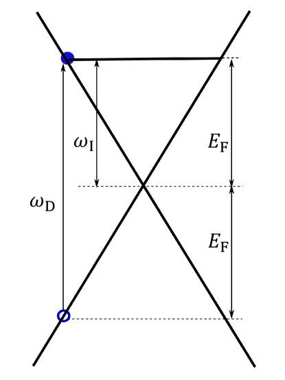
Figure 1: Band diagram of Dirac metal symmetric conduction and valence bands showing the direct (Pauli) threshold $\omega_{\mathrm{D}}=2E_{\text{F}}$ for single-particle inter-band transitions. Also shown is the indirect threshold for many-body Auger-Meitner transitions, $\omega_{\mathrm{I}}=E_{\text{F}}$.

In a typical experiment, Dirac materials are doped (gated) away from charge neutrality, either intentionally or unintentionally. From now on, we will be referring to such systems as “Dirac metals”. In this case, the Pauli principle dictates that the optical conductivity of an ideal Dirac metal is strictly zero below the “direct” (or Pauli) threshold,

$$\omega_{\mathrm{D}}=2E_{\text{F}},$$ (3)

where $E_{\text{F}}$ is the Fermi energy, measured from the Dirac point. Experimentally, however, one observes significant absorption for frequencies above the Drude tail but below $\omega_{\mathrm{D}}$ [li_dirac_2008, Mak:2008, Horng:2011, Mak:2012, Drew:2016] and significant Raman response in the same frequency range [riccardi_gate-dependent_2016], both of which indicate a deviation from the single-particle picture. Absorption below the Pauli threshold in doped graphene due to a combined effect of disorder, electron-phonon and electron-electron interaction has also been addressed theoretically in Refs. [peres2007, stauber:2008, peres:2008, peres:2010PRL]. In this paper, we focus on intrinsic absorption due to ee and electron-hole (eh) interactions for $\Omega<\omega_{\mathrm{D}}$.

Absorption due to ee interaction in a Dirac metal was studied in Refs. [Principi:2013, Sharma:2021]. For $\Omega\ll E_{\text{F}}$, the conductivity was found to scale as $\Omega^{2}\ln\Omega$ and $\Omega^{2}$ in 2D and 3D, respectively [Sharma:2021]. A quadratic scaling of the conductivity can be understood as the consequence of partially broken Galilean invariance in a Dirac-Fermi liquid (DFL). Indeed, the optical conductivity can be cast into a Drude-like form

$$\Re\sigma(\Omega)\propto\frac{1}{\Omega^{2}\tau_{j}(\Omega)},$$ (4)

where $\tau_{j}(\Omega)$ is the current relaxation time. If Galilean invariance is broken completely, e.g., by umklapp scattering, $\tau_{j}(\Omega)$ is of the same order as the quasiparticle lifetime in a Fermi liquid (FL): $\tau_{j}(\Omega)\sim\tau_{\text{qp}}(\Omega)\propto\Omega^{-2}$. In this case, Eq. (4) produces a familiar “FL foot": $\Re\sigma(\Omega)=\text{const}$. On the other hand, if Galilean invariance is intact, current cannot be relaxed in ee collisions: although $\tau_{\text{qp}}(\Omega)$ is finite, $\tau_{j}(\Omega)=\infty$ and thus $\Re\sigma(\Omega)=0$. A DFL occupies an intermediate niche between the two limits described above. On one hand, its non-parabolic spectrum allows for current relaxation; on the other hand, the spectrum is still isotropic (at low doping) and current relaxation is impossible for electrons right on the Fermi surface (FS) [Sharma:2021]. For states away from the FS, the current relaxation time is finite but long, $\tau_{j}(\Omega)\propto\Omega^{-4}$ (modulo a $\ln\Omega$ factor in 2D), while $\tau_{\text{qp}}(\Omega)$ still scales in a FL way, i.e., as $\Omega^{-2}$. According to Eq. (4), the quartic scaling of $1/\tau_{j}(\Omega)$ translates into the quadratic scaling of the conductivity.

In this paper, we extend the results of Ref. [Sharma:2021] to the entire interval of frequencies below $\omega_{\mathrm{D}}$. Such an extension necessarily requires to account for both ee and eh interaction processes. We consider 2D and 3D Dirac metals with two types of interaction: Hubbard and Coulomb. Our analytic results follow from the analysis of the Kubo formula and are applicable in two regions: i) for $\Omega\ll\omega_{\mathrm{I}}$, where

$$\omega_{\text{I}}=E_{\text{F}},$$ (5)

is the “indirect” threshold and ii) just above the indirect threshold, i.e, for $\Omega\gtrapprox\omega_{\mathrm{I}}$. In the rest of the interval $0<\Omega<\omega_{\mathrm{D}}$, the conductivity is calculated numerically, but only for a Dirac metal with Hubbard interaction. For $\Omega\ll\omega_{\mathrm{I}}$, we show that the eh contribution to the conductivity scales as $\Omega^{2}$, i.e., it is comparable to the ee one found in Ref. [Sharma:2021] in 3D and is subleading to the ee one in 2D, but only in the leading logarithm sense.

This $\Omega^{2}$-scaling of the eh contribution to the conductivity can also be understood in terms of the Drude formula (4). Current relaxation due to eh scattering is not limited by (partially broken) Galilean invariance, so that $\tau_{j}(\Omega)\sim\tau_{\text{qp}}(\Omega)\propto\Omega^{-2}$. [Unlike $\tau_{\text{qp}}(\Omega)$, $\tau_{j}(\Omega)$ does not have an extra logarithmic factor in 2D.] However, the energies of electrons and holes differ now by $E_{\text{F}}$ rather than $\Omega$; therefore, the factor of $\Omega^{2}$ in Eq. (4) is replaced by $E_{\text{F}}^{2}$, and the conductivity scales as $\Omega^{2}$.

Another channel of absorption due to eh interaction opens up when $\Omega$ exceeds the indirect threshold $\omega_{\mathrm{I}}$ [Eq. (5)]. Since the seminal 1969 paper by Gavoret et al. [gavoret_optical_1969], absorption of light by degenerate semiconductors due to a particular type of eh interaction processes, similar to Auger-Meitner (AM) processes in atomic physics [meitner:1922, Auger:1923, PhysicsToday:2019], have been studied by a large number of researchers, see, e.g., Refs. [ruckenstein_many-body_1987, Sham:1990, Hawrylak:1991, Pimenov:2017]. Although we consider only gapless systems, our result for the AM contribution just above $\omega_{\mathrm{I}}$ exhibits a threshold singularity of the same type as found for a gapped spectrum [gavoret_optical_1969, ruckenstein_many-body_1987, Sham:1990, Hawrylak:1991, Pimenov:2017], i.e.,

$$\Re\sigma(\Omega)\propto\theta(\delta\Omega)\delta\Omega^{\beta_{\text{A}}},$$ (6)

where $\delta\Omega\equiv\Omega-\omega_{\mathrm{I}}\ll\omega_{\mathrm{I}}$ and $\beta_{\text{A}}=d+2$ with $d$ being the spatial dimensionality and $\theta(x)$ is the Heaviside step function. Equation (6) can be obtained by estimating the conductivity as $\Re\sigma(\Omega)\propto\delta\Omega\mathcal{N}(\delta\Omega)/\tau_{\text{qp}}(\delta\Omega)$, where $\mathcal{N}(\epsilon)\propto\epsilon^{d-1}$ is the density of states of a gapless Dirac metal and $1/\tau_{\text{qp}}(\epsilon)\propto\epsilon^{2}$.

More important, however, is the fact that for a non-parabolic spectrum the AM contribution occurs at the background of ee and other eh contributions, which start at the lowest frequencies (as $\Omega^{2}$ and $\Omega^{2}\ln\Omega$ in 3D and 2D, respectively) and are still present both near and above $\omega_{\mathrm{I}}$. Therefore, the AM threshold singularity is masked by these other contributions. These competing contributions were not taken into account in the previous work on AM processes [gavoret_optical_1969, ruckenstein_many-body_1987, Sham:1990, Hawrylak:1991, Pimenov:2017], which considered two strictly parabolic bands separated by a gap ($2\Delta$). To clarify the difference in absorption by materials with parabolic and Dirac bands, we invoke temporarily a gapped Dirac spectrum, $\epsilon_{\textbf{k}}=\pm\sqrt{v_{\mathrm{D}}^{2}k^{2}+\Delta^{2}}$. A gapped semiconductor with parabolic conduction and valence band can be viewed as the $\Delta\to\infty$ limit of this spectrum. In this case, intra-band ee interaction does not affect the conductivity due to Galilean invariance, as we already discussed above. Moreover, inter-band absorption accompanied by electron-hole conversion processes, i.e., processes that do not conserve the numbers of electrons and holes separately, is also forbidden in the parabolic limit, because the corresponding eigenstates are either purely electron-like or purely hole-like, with zero overlap between the two. Therefore, the interaction part of the corresponding Hamiltonian conserves the numbers of electrons and holes separately, and absorption is absent for $\Omega<\omega_{\mathrm{I}}$. For a strongly non-parabolic, e.g., gapless Dirac spectrum, the ee contribution is not suppressed by Galilean invariance, while electron-hole conversion processes are generically as important as other processes.

As far as the interval of $\Omega>\omega_{\mathrm{D}}$ is concerned, Abedinpour et al. [abedinpour_drude_2011] showed that the conductivity of doped graphene (a 2D Dirac metal, in our terminology) with Coulomb interaction exhibits a logarithmic renormalization which, for $\Omega\gg\omega_{\mathrm{D}}$, is reduced to the well-studied case of undoped graphene, and is logarithmically enhanced for $\Omega\gtrapprox\omega_{\mathrm{D}}$ both for Coulomb and Hubbard interactions Both of these effects arise already at first order in the corresponding interaction and reflect renormalization of the Dirac velocity and, consequently, of the coupling constant. To the best of our knowledge, the interval of $\Omega\gg\omega_{\mathrm{D}}$ has not been studied for a 3D Dirac metal but, in analogy with the results for the undoped 3D case [Rosenstein:2013, Roy:2018], we would also expect a logarithmic renormalization starting at first order. On the other hand, absorption processes studied in our paper correspond to real collisions between electrons, and between electrons and holes, which occur starting from the second order in the interaction. Therefore, these processes are subleading to the first-order effects described above studied in Ref. [abedinpour_drude_2011], and we will not extend our results above $\omega_{\mathrm{D}}$.

Our numerical results agree with analytic ones, where applicable, and allow one to trace the behavior of the conductivity for almost entire frequency range of interest, $0<\Omega<\omega_{\mathrm{D}}$, except for a narrow interval of width $\mathcal{O}(\alpha_{\text{H,C}}^{2}E_{\text{F}})$ around $\omega_{\text{D}}$, where $\alpha_{\text{H,C}}\ll 1$ is the dimensionless coupling constant of Hubbard and Coulomb interactions, respectively. In this interval, our perturbative expansion breaks down and one needs to re-sum the diagrammatic series.

The rest the paper is organized as follows. In Sec. II, we set up the model Hamiltonians for 2D and 3D Dirac metals. In Sec. III, we outline the formalism for calculating the optical conductivity via the Kubo formula. In Sec. LABEL:sec:processes, we identify the ee and eh scattering processes that contribute to the conductivity in a given frequency range. In section LABEL:sec:archetype-conductivity, we analyze the general structure of the contributions to the conductivity from the self-energy and vertex diagrams, which serve as archetypes for other contributions. In sections LABEL:sec:3D and LABEL:sec:2Dsystems, we present our analytical and numerical results for the optical conductivity of 3D and 2D Dirac metals, respectively. Our conclusions are given in Sec. LABEL:sec:Conclusions.

II Model Hamiltonians of Dirac metals

In this section we define our model Hamiltonians for 2D and 3D Dirac metals.

II.1 3D Hamiltonian

We model a 3D Dirac metal by a $4\times 4$ low-energy Hamiltonian with two orbital degrees of freedom per spin which describes a single Dirac point [Burkov:2011, Koshino:2016, RevModPhys.90.015001]

$$\hat{\mathcal{H}}_{\text{3D}} = \hat{\mathcal{H}}_{0}+\hat{\mathcal{H}}_{\text{int}},$$ (7a)

$$\hat{\mathcal{H}}_{0} = \sum\limits_{\mathbf{k}}\Psi^{\dagger}_{\mathbf{k}}\left[v_{\mathrm{D}}\hat{\sigma}_{x}\otimes(\boldsymbol{\hat{\varsigma}}\cdot\mathbf{k})-E_{\text{F}}\hat{\sigma}_{0}\otimes\hat{\varsigma}_{0}\right]\Psi^{\phantom{}}_{\mathbf{k}},\IEEEeqnarraynumspace$$ (7b)

$$\hat{\mathcal{H}}_{\text{int}} = \frac{1}{2\mathcal{V}}\sum\limits_{\mathbf{q}}V_{\text{3D}}(\mathbf{q})\hat{n}_{\mathbf{q}}\hat{n}_{\mathbf{-q}},$$ (7c)

where $v_{\mathrm{D}}$ is the Dirac velocity, $\Psi_{\mathbf{k}}$ is the $4\times 1$ Dirac spinor, Pauli matrices $\boldsymbol{\hat{\varsigma}}=(\hat{\varsigma}_{x},\hat{\varsigma}_{y},\hat{\varsigma}_{z})$ and $\boldsymbol{\hat{\sigma}}=(\hat{\sigma}_{x},\hat{\sigma}_{y},\hat{\sigma}_{z})$ represent (real) spin and pseudospin, respectively, $\hat{\varsigma}_{0}$ and $\hat{\sigma}_{0}$ are the identity matrices in the corresponding subspaces, $\hat{n}_{\mathbf{q}}=\sum\limits_{\mathbf{k}}\Psi^{\dagger}_{\mathbf{k}}\Psi_{\mathbf{k+q}}$ is the density operator, $V_{\text{3D}}(\mathbf{q})$ is the interaction potential, and $\mathcal{V}$ is the system volume. In general, we assume that there are $N$ identical Dirac points.

The eigenvalues and orthonormal eigenfunctions of $\hat{\mathcal{H}}_{0}$ in Eq. (7b) are given by

$$\xi_{\textbf{k}}^{s}=s\epsilon_{\mathbf{k}}-E_{\text{F}},\;\epsilon_{\textbf{k}}=v_{\mathrm{D}}k$$ (8)

and lll|k,+⟩= 12 [ψ1(^ς⋅^k)ψ1] , |k,-⟩= 12[-(^ς⋅^k)ψ2ψ2],
respectively. Here $\hat{k}={\textbf{k}}/k$, $s=\pm 1$ is the helicity index, and $\psi_{1,2}$ are the $2\times 1$ spinor states such that $\psi_{1,2}^{\dagger}\psi_{1,2}=1$. We choose $\psi_{1}=\psi_{2}=(0,1)^{T}$. The Green’s function of $\hat{\mathcal{H}}_{0}$ is given by

lll^G(k,iω)=12∑_s=±^M^s_kg_s(k,iω),
^M^s_k=^σ_0⊗^ς_0+s( ^σ_x⊗(^ς⋅^k) ),
g_s(k,iω)=1iω-ξks.

For the sake of brevity, we will be omitting index $n$ in Matsubara frequencies, which will be distinguished from real ones by a factor of the imaginary unit, $i$. For example, $\omega$ in Eq. (9) stands for a Matsubara frequency. We will be referring to the bands with helicity $s=\pm 1$ as the “conduction” and “valence” bands, respectively. The density of states at the Fermi level per spin per valley is equal to $\mathcal{N}_{\text{F},3}=E_{\text{F}}^{2}/2\pi^{2}v_{\mathrm{D}}^{3}$.

The velocity operator corresponding to $\hat{\mathcal{H}}_{0}$ in (7b) is lll^v =v_D^σ_x⊗^ς with matrix elements

$${\textbf{v}}_{\textbf{k}}^{s,s^{\prime}}=\bra{\mathbf{k},s}\hat{\mathbf{v}}\ket{\mathbf{k},s^{\prime}}.$$ (10)

In what follows, we will need explicit expressions for the intra- and inter-band matrix elements of the velocity operator, which are given by lllv^s,s_k= ⟨k,s|^v|k,s⟩=s v_D^k and

$$\mathbf{v}^{+,-}_{\mathbf{k}} = \left(\mathbf{v}^{-,+}_{\mathbf{k}}\right)^{*}=\bra{\mathbf{k},+}\hat{\mathbf{v}}\ket{\mathbf{k},-}$$ (11)

$$= v_{\mathrm{D}}\psi_{1}^{\dagger}\left[\boldsymbol{\hat{\varsigma}}-\left(\boldsymbol{\hat{\varsigma}}\cdot\hat{k}\right)\boldsymbol{\hat{\varsigma}}\left(\boldsymbol{\hat{\varsigma}}\cdot\hat{k}\right)\right]\psi_{2},$$

respectively.

We now turn to the interaction part of the Hamiltonian. In what follows, we will consider two models for the interaction $V_{\text{3D}}(\mathbf{q})$:

$$[left={V_{\text{3D}}(\mathbf{q})=\empheqlbrace\,}] \lambda_{3},$$ (3D, Hubbard) (12a)

$$\frac{4\pi e^{2}}{q^{2}},$$ (3D, Coulomb) (12b)

where $\lambda_{3}>0$ is a constant and $e$ is the magnitude of electron charge. We focus on the case of low doping, when $k_{\text{F}}$ is much smaller than the distance between the nearby Dirac points, $b$. By “Hubbard interaction” we then mean an interaction that is constant for $q$ less or comparable to $k_{\text{F}}$ and falls off rapidly in the interval $k_{\text{F}}\ll q\ll b$. In that case, one can neglect scattering processes that swap electrons between the Dirac points. The Hubbard model, though not completely realistic, captures the essential physics and allows one to obtain both analytic results for the optical conductivity in certain frequency regimes and numerical results for all frequencies. Thus, we focus most of our discussion on the Hubbard model. The Coulomb model allows one to obtain analytic results in certain frequency regimes but is very expensive computationally for arbitrary frequencies, and we will restrict our analysis of this model to analytic results only. We discuss both Hubbard and Coulomb interactions in more detail in Section III.2.

Note that in the basis of electron and hole creation/annihilation operators, which diagonalizes $\hat{\mathcal{H}}_{0}$, the Hamiltonian (7c) accounts for all possible interaction processes, including those that do not conserve the number of electrons and holes. As mentioned in Sec. I, our approach is more general in this regard than the one in prior studies of optical absorption in doped semiconductors [gavoret_optical_1969, ruckenstein_many-body_1987, Sham:1990, Hawrylak:1991, Pimenov:2017]. These studies considered a model Hamiltonian, which allows only for the density-density interaction between electrons and holes

$$\hat{\mathcal{H}}^{\prime}_{\text{int}}=\frac{1}{2\mathcal{V}}\sum_{\begin{subarray}{c}{\textbf{k}},{\textbf{p}},{\textbf{q}},\\ \varsigma=\pm,s=\pm\end{subarray}}V_{\text{int}}({\textbf{q}})\hat{d}^{\dagger}_{{\textbf{k}}+{\textbf{q}},\varsigma,s}\hat{d}^{\dagger}_{{\textbf{p}}-{\textbf{q}},\varsigma^{\prime},-s}\hat{d}^{\phantom{\dagger}}_{{\textbf{p}},\varsigma^{\prime}-s}\hat{d}_{{\textbf{k}},\varsigma,s}^{\phantom{\dagger}},$$

(13)

where $\hat{d}^{\dagger}_{{\textbf{k}},\varsigma,\pm}$ is the operator creating an electron/hole with momentum k and spin $\varsigma$. Such a Hamiltonian is correct for a parabolic spectrum, in which case intra-band absorption is forbidden by Galilean invariance while processes of electron-hole conversion are absent due to the vanishing overlap of the electron and hole states. However, it is not applicable to the gapless Dirac spectrum studied in this paper.

II.2 2D Hamiltonian

As an example of a 2D Dirac metal, we consider monolayer graphene described by the standard Hamiltonian [neto:2009]:

$$\hat{\mathcal{H}}_{\text{2D}} = \hat{\mathcal{H}}_{0}+\hat{\mathcal{H}}_{\text{int}},$$ (14a)

$$\hat{\mathcal{H}}_{0} = \sum\limits_{\mathbf{k}}\Psi^{\dagger}_{\mathbf{k}}\left[v_{\mathrm{D}}\left(\tau_{z}\hat{\sigma}_{x}k_{x}+\hat{\sigma}_{y}k_{y}\right)-\hat{\sigma}_{0}E_{\text{F}}\right]\Psi_{\mathbf{k}},\IEEEeqnarraynumspace$$ (14b)

$$\hat{\mathcal{H}}_{\text{int}} = \frac{1}{2\mathcal{V}}\sum\limits_{\mathbf{q}}V_{\text{2D}}(\mathbf{q})\hat{n}_{\mathbf{q}}\hat{n}_{\mathbf{-q}},$$ (14c)

where $\tau_{z}=\pm 1$, $\Psi_{\mathbf{k}}$ is a $2\times 1$ Dirac spinor, the set of Pauli matrices $\hat{\boldsymbol{\sigma}}=(\hat{\sigma}_{x},\hat{\sigma}_{y},\hat{\sigma}_{z})$ describes pseudospin, $\hat{\sigma}_{0}$ is the identity matrix in the same subspace, $\hat{n}_{\mathbf{q}}=\sum\limits_{\mathbf{k}}\Psi^{\dagger}_{\mathbf{k}}\Psi_{\mathbf{k+q}}$ is the density operator, and $\mathcal{V}$ is the system area. To use the large-$N$ approximation afterwards, we assume that fermions carry spin $\varsigma$, such that the total degeneracy is $N=2(2\varsigma+1)$.

The eigenvalues of $\hat{\mathcal{H}}_{0}$ in Eq. (14b) are the same as in Eq. (8), while its orthonormal eigenfunctions are given by lll|k,+⟩= 12[1τzeiτzϕk] , |k,-⟩= 12 [-τze-iτzϕk, 1 ]
where $\phi_{\textbf{k}}$ is the azimuthal angle of k. The Green’s function of $\hat{\mathcal{H}}_{0}$ is given by

lll^G(k,iω)=12∑_s=±^M^s_kg_s(k,iω),
^M^s_k=^σ_0+s(v_D^σxτzkx+^σykyϵk ),

where $g_{s}({\textbf{k}},i\omega)$ is the same as in Eq. (9). The density of states at the Fermi level per spin per valley is equal to $\mathcal{N}_{\text{F},2}=E_{\text{F}}/2\pi v_{\mathrm{D}}^{2}$.

The velocity operator corresponding to $\hat{\mathcal{H}}_{0}$ is lll^v =v_D(τ_z^σ_x,^σ_y), with its intra-band matrix element being the same as in Eq. (II.1), while the inter-band matrix element is given by lllv^+,-_k&=(v^-,+_k)^*=⟨k,+|^v|k,-⟩
=iv_D e^-iτ_zϕ_k (^k×^z), where $(\hat{x},\hat{y},\hat{z})$ are the Cartesian unit vectors. As in 3D, the intra- and inter-band velocities are orthogonal to each other.

Lastly, similar to the 3D case, we consider two models of the interaction

$$[left={V_{\text{2D}}(\mathbf{q})=\empheqlbrace\,}] \lambda_{2},$$ (2D, Hubbard) (16a)

$$\frac{2\pi e^{2}}{q},$$ (2D, Coulomb) (16b)

where $\lambda_{2}>0$ is a constant. As in 3D, by “Hubbard” interaction we mean the interaction with radius shorter than the Fermi wavelength but longer that the lattice constant, which cannot transfer electrons between the valleys. As in 3D, we will present both the analytical and numerical results for the Hubbard case, and only the analytical results for the Coulomb case.

III Optical conductivity: general formalism

III.1 Kubo formula

In linear response, the real part of the optical conductivity is given by the Kubo formula lllℜσ_αβ( Ω)= -1ΩℑΠ_αβ,R(Q=0,Ω), where $\alpha,\beta=x,y(z)$ in 2D and 3D, respectively, and $\Pi_{\alpha\beta\text{,R}}(\mathbf{Q=0},\Omega)$ is the retarded current-current correlation function (denoted by subscript “R"), which is obtained by analytic continuation of its Matsubara counterpart: lllΠ_αβ,R(Q,Ω)=Π_αβ(Q,iΩ→Ω+i0^+),
Π_αβ(Q,iΩ)=-1V∫_0^1/k_BTdτe^iΩτ⟨T_τ^j_α^†(Q,τ)^j_β(Q,0)⟩.
In the basis of conduction/valence bands, the current operator is written as lll^j(Q,τ)=-e∑_k,s,s’v^s,s’_k ^d^†_k-Q2,s(τ)^d^_k+Q2,s’(τ), where ${\textbf{v}}_{{\textbf{k}}}^{s,s^{\prime}}$ is given by Eq. (10).

For isotropic systems, considered in this paper, the conductivity tensor is diagonal and symmetric. In this case, we define

$$\Pi(\mathbf{Q},i\Omega) \equiv \frac{1}{d}\sum\limits_{\alpha}\Pi_{\alpha\alpha}(\mathbf{Q},i\Omega),$$

$$\Pi_{\text{R}}(\mathbf{Q},\Omega) \equiv \frac{1}{d}\sum\limits_{\alpha}\Pi_{\alpha\alpha,\text{R}}(\mathbf{Q},\Omega),$$

$$\Re\sigma(\Omega) = -\frac{1}{\Omega}\Im\Pi_{\text{R}}(\mathbf{Q=0},\Omega).$$ (17)

We also assume that temperature is much smaller than any other energy scale of the problem and consider only the $T=0$ limit.

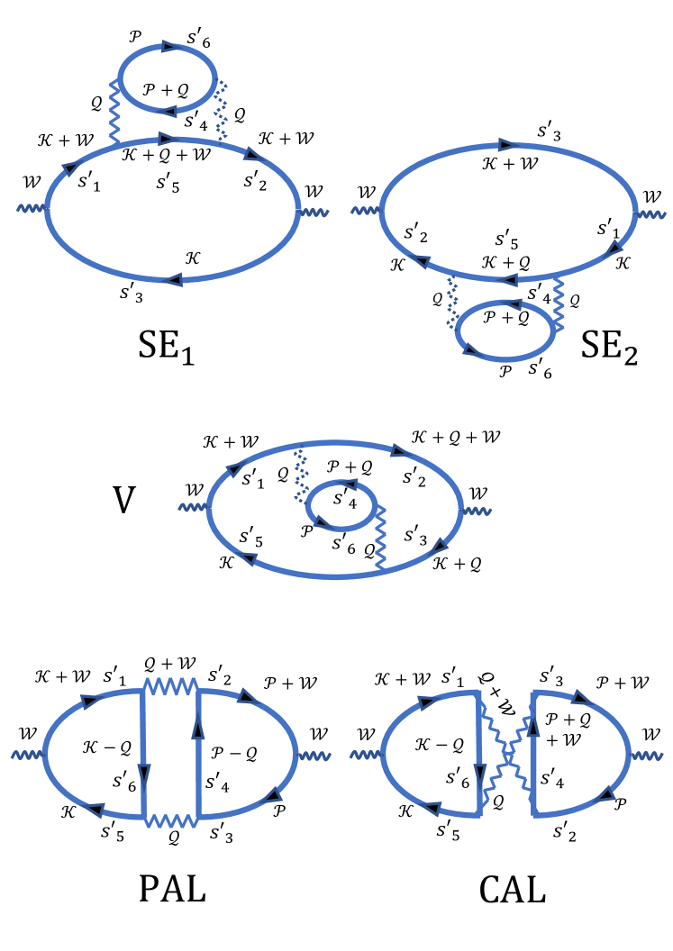
Figure 2: Leading-order diagrams for the current-current correlation function. Thick solid lines depict the matrix Green’s functions, given by Eqs. (9) and (15) in 3D and 2D, respectively. For Hubbard interaction, the solid and broken wavy lines are identical and depict the Hubbard interaction $\lambda_{d}=\text{const}$ in $d$ dimensions, and the displayed diagrams are the leading ones in the large $N$-approximation. For Coulomb interaction, the solid and broken wavy lines depict the dynamically and statically screened Coulomb potentials, respectively [Eqs. (III.2.2), (22a), (22b)], and the displayed diagrams are the leading ones within the random-phase approximation. The external momentum has only the frequency component: $\mathcal{W}=({\bf 0},i\Omega)$. From top to bottom: self-energy (SE₁ and SE₂), vertex (V), parallel (PAL) and crossed Aslamazov-Larkin (CAL) diagrams. Indices $s^{\prime}_{1}\dots s^{\prime}_{6}=\pm 1$ indicate helicities that are being summed over.

III.2 Relevant diagrams

In Dirac metals, optical absorption occurs already for non-interacting particles, if the frequency of incident light exceeds the direct threshold, $\omega_{\mathrm{D}}=2E_{\text{F}}$. The main focus of this paper is the range of $0<\Omega<2E_{\text{F}}$, where absorption occurs only if electrons interact with other degrees in freedom, in particular, both among themselves and with holes. Dissipation occurs only if the interaction is dynamic, i.e., if the bare interaction, either Hubbard or Coulomb, is dressed by particle-hole pairs. Diagrammatically, this corresponds to renormalizing the interaction lines either by particle-hole polarization bubbles or “Aslamazov-Larkin triangles” (cf. Fig. 2).

III.2.1 Hubbard interaction

To make the analysis tractable, we assume that the number of identical Dirac points is large ($N\gg 1$) and also adopt the weak-coupling approximation, i.e, we assume that $\alpha_{\text{H}}N\ll 1$, where

$$\alpha_{\text{H}}=\lambda_{d}\mathcal{N}_{\text{F},d}$$ (18)

is the dimensionless coupling constant. The first assumption allows us to retain only diagrams with the highest number of fermion loops, while the second one allows us to keep the lowest order in the interaction at which dissipation occurs, to wit: the second. The relevant diagrams for the current-current correlation function are shown in Fig. 2. For the Hubbard case, the solid and broken interaction lines are identical and denote the Hubbard coupling $\lambda_{d}$.

III.2.2 Coulomb interaction

Within the random-phase approximation (RPA), the dynamically screened Coulomb interaction is given by lllV(q,iν)=1V-10(q)+π0(q,iν) where

$$\pi_{0}({\textbf{q}},i\nu)=-\int_{\mathcal{K}}\operatorname{Tr}\left[\hat{G}({\textbf{k}}+{\textbf{q}},i\omega+i\nu)\hat{G}({\textbf{k}},i\omega)\right],$$ (19)

is the polarization bubble, $\int_{\mathcal{K}}$ is a short-hand for $(2\pi)^{-(d+1)}\int\text{d}^{d}k\int\text{d}\omega$, and $\hat{G}$ is the free-electron Green’s function given by Eqs. (9) and (15) in 3D and 2D, respectively. Since only the dynamic interaction contributes to dissipation, it is convenient to subtract off the static part of the interaction and treat the remaining dynamic part as the effective interaction. The dynamic part is given by

$$V_{\text{dyn}}(\mathbf{q},i\nu) \equiv V({\textbf{q}},i\nu)-V({\textbf{q}},0)$$ (20)

$$= -V(\mathbf{q},i\nu)V(\mathbf{q},0)\pi_{0,\text{dyn}}(\mathbf{q},i\nu),$$

where lllπ_0,dyn(q,iν)=π_0(q,iν)-π_0(q,0)is the dynamic part of the polarization bubble. The lowest two-loop order diagrams in $V_{\text{dyn}}(\mathbf{q},i\nu)$ are shown in Fig. 2, where now the solid and broken wavy lines depict the dynamic and static parts of the interaction, respectively.

As opposed to the Hubbard case, the Coulomb one has an additional energy scale, lllω_pd= v_Dκ_d,where

$$\kappa_{3}=\left(4\pi e^{2}N\mathcal{N}_{\text{F},3}\right)^{1/2}$$ (21a)

and

$$\kappa_{2}=2\pi e^{2}N\mathcal{N}_{\text{F},2}$$ (21b)

are the inverse screening radii in 3D and 2D, respectively. For $d=3$, $\omega_{\text{p}3}$ is on the order of the plasmon frequency at $q=0$. For $d=2$, $\omega_{\text{p}2}$ is on the order of the plasmon dispersion evaluated at $q\sim\kappa_{2}$. The condition for the Coulomb interaction to be treated via within RPA is $\kappa_{d}\ll k_{\text{F}}$, which implies that $\omega_{\text{p}d}\ll E_{\text{F}}$. Correspondingly, the frequency region $0<\Omega\ll E_{\text{F}}$ is divided into two subregions: $0<\Omega\ll\omega_{\text{p}d}$ and $\omega_{\text{p}d}\ll\Omega\ll E_{\text{F}}$. In the first subregion, a typical energy transfer, $\nu$, is on the order of $\Omega$, while a typical momentum transfer, $q$, is on the order of $\kappa_{d}$. Therefore, $\nu\ll v_{\mathrm{D}}q\sim\omega_{\text{p}d}$. In this case, one can set $\nu=0$ in the first factor on the RHS of Eq. (20) with the result lllV_dyn(q,iν)≈-V^2(q,0) π_0,dyn(q,iν). Diagrammatically, this amounts to replacing all the solid wavy lines by broken wavy ones in Fig. 2. Because $q\ll k_{\text{F}}$, the static screened potential is described by the usual Thomas-Fermi form:

$$[left={V(\mathbf{q},0)=\empheqlbrace\,}] \frac{4\pi e^{2}}{q^{2}+\kappa_{3}^{2}},$$ for 3D (22a)

$$\frac{2\pi e^{2}}{q+\kappa_{2}}, \text{for 2D}.$$ (22b)

In the second subregion ($\omega_{\text{p}d}\ll\Omega\ll E_{\text{F}}$), typical energy and momentum transfers are $\nu\sim v_{\mathrm{D}}q\sim\Omega\gg\omega_{\text{p}d}$. In this case, screening is irrelevant and the effective dynamic interaction is given by

$$V_{\text{dyn}}({\textbf{q}},i\nu)=-V^{2}_{0}({\textbf{q}})\pi_{0,\text{dyn}}({\textbf{q}},i\nu),$$ (23)

where $V_{0}({\textbf{q}})$ is the bare Coulomb potential.

Note that we do not need to use the large-$N$ approximation for the Coulomb case, it is enough to require that the dimensional coupling constant of the Coulomb interaction

$$\alpha_{\text{C}}=\frac{v_{\mathrm{D}}\kappa_{d}}{E_{\text{F}}}$$ (24)

is small, which is the condition for the validity of RPA. For the Coulomb case, therefore, we will restrict our analysis to the actual value of $N$ for a specific system.

III.3 Current-current correlation function on the Matsubara axis

In this section, we describe the general structure of the diagrams for the current-current correlation function. The set of diagrams in Fig. 2 includes two self-energy (SE) diagrams, SE₁ and SE₂, a vertex correction diagram (V), and two Aslamazov-Larkin (AL) diagrams in the particle-particle and particle-hole channels, labelled as PAL (“parallel AL”) and CAL (“crossed AL”), respectively. The contributions of individual diagrams to the current-current correlation function at the external $d+1$ momentum $\mathcal{W}\equiv({\bf 0},i\Omega)$ are given by

lllΠ^SE_1(W)=1d∫_KTr[^v ^S(K+W)⋅^v ^G(K)],
Π^SE_2(W)=1d∫_KTr[^v ^G(K+W)⋅^v ^S(K)],
Π^V(W)=1d∫_K’Tr[^Γ (K’;W)^G(K’+W)⋅^v ^G(K’)],

Π^PAL(W)=-1d∫_QV^2_st( q) A(Q,W)⋅B(Q,W),
Π^CAL(W)=-1d∫_QV^2_st (q) A(Q,W)⋅C(Q,W),

where

lll^S(L)=^G(L)^Σ(L)^G(L),
^Σ(L)=-∫_Q~V(Q)^G(L+Q),
~V(Q)=-V_st^2(q)π_0(Q),
^Γ (K’;W)=-∫_K~V(K’-K)^G(K)^v ^G(K+W),
A (Q,W)=-∫_KTr[^G(K)^v ^G(K+W)^G(K-Q)],
B (Q,W)=-∫_PTr[^G(P+W)^v ^G(P)^G(P-Q)],
C (Q,W)=-∫_PTr[^G(P)^G(P+W+Q)^G(P+W)^v ],

$\mathcal{K}\equiv(\mathbf{k},i\omega)$, $\mathcal{K^{\prime}}\equiv(\mathbf{k^{\prime}},i\omega)$, $\mathcal{P}\equiv(\mathbf{p},i\omega)$, $\mathcal{Q}\equiv(\mathbf{q},i\nu)$, $\pi_{0}(\mathcal{Q})$ is defined by Eq. (19), and $V_{\text{st}}(\mathbf{q})$ is the static part of the interaction, equal to $V(\mathbf{q},0)$ [Eqs. (22a) and (22b)] and to $\lambda_{d}$ for the Coulomb and Hubbard cases, respectively. The expressions above are valid for Coulomb interaction at the lowest frequencies ($\Omega\ll E_{\text{F}}$) and for any frequency for Hubbard interaction. Using the free rather than dressed Green’s functions is justified for any frequency except for a narrow region near the direct threshold (a precise condition will be formulated later, cf. Sec. LABEL:sec:IF3D). The total current-current correlation function is the sum of all the contributions displayed above: lllΠ(W)=∑_JΠ^J(W), where $J\in\{\text{SE},\text{V},\text{PAL},\text{CAL}\}$, and “SE” refers to both the self-energy diagrams collectively.

Equations (25)-(25) become more transparent if written in the electron-hole basis, in which $\hat{\mathcal{H}}_{0}$ is diagonal. Indeed, any diagram contains six Green’s functions, each being the sum of an electron and hole parts with helicities $s^{\prime}=\pm 1$, respectively. This gives rise to a set of six helicities $\mathcal{S}^{\prime}=\{s^{\prime}_{1}\dots s^{\prime}_{6}\}$ that are to be summed over. Thus, each diagram is the sum of $2^{6}=64$ terms lllΠ^J(W)=∑_S’ Π^J