Completeness of trajectories associated to Appell hypergeometric functions

Abstract.

We examine the linear completeness of trajectories of eigenfunctions associated to non-linear eigenvalue problems, subject to Dirichlet boundary conditions on a segment. We pursue two specific goals. On the one hand, we establish that linear completeness persists for the non-linear Schrödinger equation, even when the trajectories lie far from those of the linear equation where bifurcations occur. On the other hand, we show that this is also the case for a fully non-linear version of this equation which is naturally associated with Appell hypergeometric functions. Both models shed new light on a framework for completeness in the non-linear setting, considered by L.E. Fraenkel over 40 years ago, that may have significant potential but which does not seem to have received much attention.

1. Introduction

In two consecutive papers [7, 8] published at the end of the 1970s which appear to have been largely overlooked, L.E. Fraenkel considered the questions of linear and non-linear completeness for a family of trajectories on a Hilbert space. Taking as one of two models for his investigations the semi-linear eigenvalue problem

(1) $$u^{\prime\prime}-u^{3}+\lambda u=0$$

$$u(0)=u(1)=0,$$

he established among several other remarkable results, that a collection of eigenfunctions $\{u_{n}\}_{n=1}^{\infty}\equiv\{u_{n}\}$ of (1) is linearly complete in $L^{2}(0,1)\equiv L^{2}$, when subject to a control on the growth of the norms of the $u_{n}$.

In terms of the Jacobi elliptic functions, $\operatorname{sn}(y,\mu)$, this family is given explicitly by

(2) $$u(x)=u_{n}(x,\mu)=2^{\frac{3}{2}}n\mu K(\mu)\operatorname{sn}(2K(\mu)nx,\mu)$$

with associated eigenvalues

$$\lambda=\lambda_{n}=4n^{2}(1+\mu^{2})K(\mu)^{2}.$$

Here the modulus $\mu$ lies in $(0,1)$ and it is a free parameter, while the 1/4 period $K(\mu)$ is the complete elliptic integral. According to [7, Theorem 3.3(i)], if $\{\mu_{n}\}_{n=1}^{\infty}\subset(0,1)$ is a sequence for which

(3) $$\{\|u_{n}(\cdot,\mu_{n})\|/n\}\in\ell^{4}(\mathbb{N}),$$

then $\{u_{n}\}$ is a basis of $L^{2}$.

A key component in the proof of this result, is the fact that (3) is equivalent to the condition

$$\sum_{n=1}^{\infty}\left\|\frac{u_{n}(\cdot,\mu_{n})}{n\gamma_{n}}-e_{n}\right\|^{2}<\infty$$

for $e_{n}(x)=2^{\frac{1}{2}}\sin(n\pi x)$ and $\gamma_{n}$ the $n$-th sine Fourier coefficient of $u_{n}/n$. This is known to be sufficient, but not necessary, for $\{u_{n}\}$ to become a basis of $L^{2}$. Moreover, although it allows $\|u_{n}(\cdot,\mu_{n})\|$ to be $O(n^{c})$ as $n\to\infty$ for all $c<3/4$, (3) holds if and only if $\{\mu_{n}\}\in\ell^{4}(\mathbb{N})$. Therefore, it requires $\mu\to 0$. In this regime, the equation (1) bifurcates from the linear eigenvalue equation and it is natural to expect that $\{u_{n}\}$ is close enough to an orthonormal basis of $L^{2}$.

The present paper is devoted to two specific goals in the context of Fraenkel’s original idea of asking questions about linear and non-linear completeness for trajectories of eigenfunctions. On the one hand, we show that $\{u_{n}\}$ is also a basis for any $\{\mu_{n}\}\subset(0,1)$ such that $\limsup\mu_{n}\leq\mu_{0}$, where $\mu_{0}<1$ is a constant very close to 1. Concretely, we show that $\{u_{n}/n\}$ is a Riesz basis in the sense that it is equivalent to the orthonormal basis $\{e_{n}\}$. On the other hand, we examine linear completeness on a fully non-linear version of (1). The eigenvalue equation

(4) $$(\operatorname{sgn}(\phi^{\prime})|\phi^{\prime}|^{p-1})^{\prime}-(p-1)\operatorname{sgn}(\phi)|\phi|^{2p-1}+\lambda(p-1)\operatorname{sgn}(\phi)|\phi|^{p-1}=0$$

$$\phi(0)=\phi(1)=0,$$

for $p>1$, in which we have replaced the Laplacian term by the non-linear $p$-Laplacian.

This new equation is neither artificial nor it is a purposeless generalisation of (1). Rather, it provides a natural link between the framework of the papers [7, 8] and the one developed recently for the $p$-Laplacian and other families of dilated periodic functions arising in the context of Sobolev embeddings on the segment. A systematic treatment of the latter can be found in the book [6] and the state-of-the-art on the basis question for the $p$-Laplacian and other related non-linear operators can be found in the papers [4] and [2]. For a full list of updated references on the subject and a more general perspective, see also the paper [3].

We thank Domenic Petzinna for his useful comments and attentive reading of an earlier version of this manuscript, and Shingo Takeuchi for telling us about the work [11, 12]. The background to the concepts and terminology employed below can be found in the books [9] and [14].

2. The eigenvalue equation

Let $p>1$. We examine families of solutions to (4). The case $p=2$ corresponds to (1). Our interest is completeness properties near and far from bifurcation phenomena associated to the $p$-Laplacian eigenvalue equation

(5) $$(\operatorname{sgn}(\phi^{\prime})|\phi^{\prime}|^{p-1})^{\prime}+\lambda(p-1)\operatorname{sgn}(\phi)|\phi|^{p-1}=0$$

$$\phi(0)=\phi(1)=0.$$

We know that the eigenfunctions of (5) become a Riesz basis of $L^{2}$ for all $p>p_{0}$, where $p_{0}>1$ is a constant close to 1. Specific characterisations of $p_{0}$ can be found in [4, Theorem 4.5] and [2, Theorem 6.5].

Solutions to (4) are given in terms of inverse Appell hypergeometric functions, as follows. For (general) modulus $\mu\in(0,1)$, let

$$K_{p}(\mu)=\int_{0}^{1}(1-s^{p})^{-\frac{1}{p}}(1-\mu^{p}s^{p})^{-\frac{1}{p}}\,\mathrm{d}s$$

and let $\operatorname{sn}_{p}(y,\mu)$ be the odd $4K_{p}(\mu)$-periodic continuous extension of the inverse function of

$$w_{p}(z)=\int_{0}^{z}(1-s^{p})^{-\frac{1}{p}}(1-\mu^{p}s^{p})^{-\frac{1}{p}}\,\mathrm{d}s.$$

Then, $\operatorname{sn}_{p}(y,\mu)$ is positive and increasing for $y\in\big{(}0,K_{p}(\mu)\big{)}$. The re-scaled function $\operatorname{sn}_{p}(2K_{p}(\mu)x,\mu)$ is 2-periodic, odd and differentiable. It is positive on $(0,1)$ with maximum value equal to 1 at $x=\frac{1}{2}$. It is also even with respect to that point. The notation we employ here is consistent with that of the paper [11].

A full description of the eigenvalues and eigenfunctions for non-linear equations such as (4), and an analysis of the bifurcation phenomenona around those of (5), was established in the paper [13]. See also [11]. If $1<p\leq 2$, a full set of eigenfunctions of (4) is given by dilations of $\operatorname{sn}_{p}(2K_{p}(\mu)x,\mu)$, for suitable $\lambda>0$. By contrast, for $p>2$, a full set of eigenfunctions for large $\lambda$ also includes the possibility of sub-segments of $(0,1)$ where $\phi(x)$ is constant. The crucial distinction between the two cases is the fact that $\lim_{\mu\to 1}K_{p}(\mu)=\infty$ if and only if $1<p\leq 2$.

In the present manuscript we will only consider trajectories of solutions which are not locally constant, as described in the following theorem.

Theorem 1.

Let $p>1$. A differentiable function $\phi:\mathbb{R}\longrightarrow\mathbb{R}$, such that $\phi$ is not constant on any open segment, satisfies the equation (4) for some $\lambda>0$ if and only if the following holds true. For a unique pair $(\mu,n)\in(0,1)\times\mathbb{N}$,

$$\phi(x)=\pm 2^{\frac{p+1}{p}}n\mu K_{p}(\mu)\operatorname{sn}_{p}(2nK_{p}(\mu)x,\mu)$$

and

$$\lambda=2^{p}n^{p}(1+\mu^{p})K_{p}(\mu)^{p}.$$

Here $n$ determines the number of zeros of the eigenfunction in the segment $(0,1)$ and, alongside with $\mu$ and $p$, it determines its norm. This stametent is a direct consequence of [13, Theorem 2.1] for $1<p\leq 2$ and [13, Theorem 2.2] for $p>2$. We give details of the proof.

Proof.

We focus on the “only if” part of the proof. The “if” part may be checked by direct substitution, but it can be better confirmed by reversing the arguments below.

Let $\phi(x)$ and $\lambda>0$, be such that (4) holds and $\phi(x)>0$ for all $x\in(0,1)$. Then,

$$[(\phi^{\prime})^{p-1}]^{\prime}-(p-1)\phi^{2p-1}+\lambda(p-1)\phi^{p-1}=0,$$

$$\phi(0)=\phi(1)=0.$$

Multiplying each term of this equation by $\frac{p}{p-1}\phi^{\prime}$, yields

$$\frac{p}{p-1}\phi^{\prime}[(\phi^{\prime})^{p-1}]^{\prime}=[(\phi^{\prime})^{p}]^{\prime},\qquad\frac{p}{p-1}\phi^{\prime}(p-1)\phi^{2p-1}=\frac{1}{2}(\phi^{2p})^{\prime}$$

and

$$\frac{p}{p-1}\phi^{\prime}\lambda(p-1)\phi^{p-1}=\lambda(\phi^{p})^{\prime}.$$

Then,

$$(\phi^{\prime})^{p}=\frac{1}{2}\phi^{2p}-\lambda\phi^{p}+c^{p}=\frac{1}{2}(\alpha-\phi^{p})(\beta-\phi^{p})$$

for $c=\phi^{\prime}(0)>0$ and

$$\alpha,\,\beta=\lambda\pm\sqrt{\lambda^{2}-2c^{p}}.$$

Here $\alpha$ picks the ‘$+$’ sign and $\beta$ the ‘$-$’ sign. Hence,

(6) $$\phi^{\prime}=2^{-\frac{1}{p}}\left[(\alpha-\phi^{p})(\beta-\phi^{p})\right]^{\frac{1}{p}}.$$

Since $\phi(0)=\phi(1)=0$, there exists $x_{0}\in(0,1)$ such that $\phi^{\prime}(x_{0})=0$. As $\phi$ is positive by our assumption, it is then increasing from $x=0$. That is, $\phi^{\prime}(x)>0$ for all $x\in[0,x_{0})$ and $0<\beta\leq\alpha$ (both roots should be positive and real). Also,

$$\phi^{p}(x_{0})=\beta>0\qquad\text{and}\qquad\lambda^{2}\geq 2c^{p}>0.$$

Let $a^{p}=\alpha$ and $b^{p}=\beta$. Integrating (6), gives

$$x=\int_{0}^{\phi}(a^{p}-t^{p})^{-\frac{1}{p}}(b^{p}-t^{p})^{-\frac{1}{p}}\,\mathrm{d}t$$

for $0\leq x(\phi)\leq x_{0}$ and $0\leq\phi(x)\leq b$, both increasing. Writing

$$x=\frac{2^{\frac{1}{p}}}{ab}\int_{0}^{\phi}\left(1-\left(\frac{t}{a}\right)^{p}\right)^{-\frac{1}{p}}\left(1-\left(\frac{t}{b}\right)^{p}\right)^{-\frac{1}{p}}\,\mathrm{d}t$$

and changing variables to $s=\frac{t}{b}$, then calling $\mu=\frac{b}{a}$, gives

$$x=\frac{2^{\frac{1}{p}}}{a}\int_{0}^{\frac{\phi}{b}}(1-\mu^{p}s^{p})^{-\frac{1}{p}}(1-s^{p})^{-\frac{1}{p}}\,\mathrm{d}s.$$

Hence, with $w_{p}(z)$ as above,

$$w_{p}\left(\frac{\phi(x)}{b}\right)=\frac{ax}{2^{\frac{1}{p}}}.$$

The function $\phi(x)$ attains its maximum at $x=x_{0}$ and $\phi(x_{0})=b$. With the definition of $K_{p}(\mu)$ as above, this gives

$$K_{p}(\mu)=\frac{ax_{0}}{2^{\frac{1}{p}}}.$$

Now, by virtue of [13, Theorem 2.1] for $1<p\leq 2$ or [13, Theorem 2.2] for $p>2$ where for the latter we use the hypothesis that $\phi$ is not constant on any open segment, it follows that $\phi$ is even with respect to $x_{0}$. Then, $\phi(2x_{0})=0$. But, because $2x_{0}$ is the first zero of $\phi$, then necessarily $x_{0}=\frac{1}{2}$. Thus

$$a=2^{\frac{p+1}{p}}K_{p}(\mu).$$

Therefore, recalling that $b=a\mu$, we have

$$\phi(x)=b\operatorname{sn}_{p}\left(\frac{ax}{2^{\frac{1}{p}}},\mu\right)=2^{\frac{p+1}{p}}K_{p}(\mu)\mu\operatorname{sn}_{p}\left(2K_{p}(\mu)x,\mu\right)$$

where $\operatorname{sn}_{p}(y,\mu)$ is the inverse function of $w_{p}(z)$ as defined above.

This determines the expression for a positive eigenfunction $\phi(x)$ as stated in the theorem (that is for $n=1$) and it also shows that this eigenfunction is unique. Moreover, since

$$\lambda=\frac{a^{p}+b^{p}}{2}=2^{p}(1+\mu^{p})K_{p}(\mu)^{p},$$

we also obtain the expression for the eigenvalue. So, we know that the eigenpair $(\phi,\lambda)$ is determined uniquely from the pair $(\mu,1)\in(0,1)\times\mathbb{N}$, when $\phi$ is positive.

The claimed statements for $n\geq 2$ follow by evaluating the equation at $n\phi(nx)$. The solution is unique, assuming $\phi^{\prime}(0)>0$ from [13, Theorem 2.1] for $1<p\leq 2$, and from [13, Theorem 2.2] for $p>2$ additionally assuming that $\phi$ is not locally constant. The two signs choice in the conclusion is a consequence of the fact that if $\phi(x)$ is an eigenfunction, then also $-\phi(x)$ is. ∎

Note that

(7) $$K_{p}(\mu) =\int_{0}^{1}\frac{x^{\frac{1}{p}-1}}{p}(1-x)^{-\frac{1}{p}}(1-\mu^{p}x)^{-\frac{1}{p}}\,\mathrm{d}x$$

$$=\frac{\operatorname{B}\left(\frac{1}{p},\frac{1}{p^{\prime}}\right)}{p}\ _{2}\!\operatorname{F}_{1}\left(\frac{1}{p},\frac{1}{p};1,\mu^{p}\right)$$

and

$$w_{p}(z)=zF_{1}\left(\frac{1}{p},\frac{1}{p},\frac{1}{p},\frac{p+1}{p};z^{p},\mu^{p}z^{p}\right).$$

Therefore, $w_{p}(z)$ is given in terms of Appell hypergeometric functions [5].

Turning back to the function $\operatorname{sn}_{p}(y,\mu)$, let us describe some of its structural properties. Since

$$\frac{\mathrm{d}(\operatorname{sn}_{p}(y,\mu))}{\mathrm{d}y}=(1-[\operatorname{sn}_{p}(y,\mu)]^{p})^{\frac{1}{p}}(1-\mu^{p}[\operatorname{sn}_{p}(y,\mu)]^{p})^{\frac{1}{p}}$$

for all $y\in[0,K_{p}(\mu)]$, then $\operatorname{sn}_{p}(y,\mu)$ and its periodic extension are continuously differentiable on $\mathbb{R}$. Moreover,

$$\frac{\mathrm{d^{2}}(\operatorname{sn}_{p}(y,\mu))}{\mathrm{d}y^{2}}=h_{p}(\operatorname{sn}_{p}(y,\mu))$$

where

$$h_{p}(z)=z^{p-1}(1-z^{p})^{\frac{2}{p}-1}(1-\mu^{p}z^{p})^{\frac{2}{p}-1}((\mu^{p}+1)z^{p}-2)<0$$

for all $z\in(0,1)$. Then, for the periodic extension (and $p\not=2$), $\operatorname{sn}_{p}^{\prime\prime}(y,\mu)<0$ for $y\in[0,K_{p}(\mu))$ and $\operatorname{sn}_{p}^{\prime\prime}(y,\mu)>0$ whenever $y\in(K_{p}(\mu),2K_{p}(\mu)]$. At the 1/4-period $y=K_{p}(\mu)$ and at its odd integer multiples, the second derivative is continuous for all $1<p\leq 2$ but it has a singularity for all $p>2$. Nonetheless, this second derivative is always locally $L^{1}$, because

$$\int_{K_{p}(\mu)-\epsilon}^{K_{p}(\mu)+\epsilon}\!|\operatorname{sn}_{p}^{\prime\prime}(y,\mu)|\,\mathrm{d}y=-\operatorname{sn}_{p}^{\prime}(y,\mu)\Big{|}_{y=K_{p}(\mu)-\epsilon}^{y=K_{p}(\mu)}\!\!\!+\operatorname{sn}_{p}^{\prime}(y,\mu)\Big{|}_{y=K_{p}(\mu)}^{y=K_{p}(\mu)+\epsilon}\!\!\!<\infty.$$

That is,

(8) $$\operatorname{sn}_{p}^{\prime\prime}(\cdot,\mu)\in\begin{cases}C(\mathbb{R})&1<p\leq 2\\ L^{1}_{\mathrm{loc}}(\mathbb{R})&p>2.\end{cases}$$

All these basic properties will be invoked in the proof of our main theorem below.

The next lemma can be regarded as a version of the classical Jordan Inequality. The case corresponding to $\mu=0$ was established in [4, Proposition 2.3].

Lemma 1.

For all $y\in\left(0,K_{p}(\mu)\right)$,

$$\frac{1}{K_{p}(\mu)}\leq\frac{\operatorname{sn}_{p}(y,\mu)}{y}\leq 1.$$

Proof.

Changing variables to $s=zr$ in the integral defining $w_{p}(z)$, yields

$$w_{p}(z)=z\int_{0}^{1}(1-y^{p}r^{p})^{-\frac{1}{p}}(1-\mu^{p}z^{p}r^{p})^{-\frac{1}{p}}\,\mathrm{d}r.$$

Then, substituting $y=w_{p}(z)$, gives

$$y=\operatorname{sn}_{p}(y,\mu)\int_{0}^{1}(1-\operatorname{sn}_{p}^{p}(y,\mu)r^{p})^{-\frac{1}{p}}(1-\mu^{p}\operatorname{sn}_{p}^{p}(y,\mu)r^{p})^{-\frac{1}{p}}\,\mathrm{d}r.$$

Denote the integral on the right hand side by $A$. Since $0<\operatorname{sn}_{p}(y,\mu)<1$, we conclude that

$$1\leq A\leq\int_{0}^{1}(1-r^{p})^{-\frac{1}{p}}(1-\mu^{p}r^{p})^{-\frac{1}{p}}\,\mathrm{d}r=K_{p}(\mu).$$

∎

For $\underline{\mu}=\{\mu_{n}\}_{n=1}^{\infty}\in(0,1)^{\infty}$, we write

$$f_{n}(x)\equiv f_{n,\underline{\mu}}(x)=\operatorname{sn}_{p}(2K_{p}(\mu_{n})nx,\mu_{n}).$$

Whenever it is sufficiently clear from the context, we leave implicit the dependence of $\{f_{n}\}$ on $\underline{\mu}$. Then,

$$\phi_{n}(x)=2^{\frac{p+1}{p}}\mu_{n}nK_{p}(\mu_{n})f_{n}(x)$$

form a collection of eigenfunctions of (4), for $n\in\mathbb{N}$. Our next statement is the first main contribution of this paper. It gives sufficient conditions on $\underline{\mu}$ for $\{f_{n,\underline{\mu}}\}$ to be a Riesz basis of $L^{2}(0,1)$.

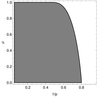
Figure 1. In the shaded region, $K_{p}(\mu)<\frac{8}{\pi^{2}-8}$. The numerical approximations employed might not be too accurate for $\mu$ near 1. But away from that region, the graph gives a sharp approximation illustrating the interplay between the two parameters for the conclusion of Theorem 2 to hold true.

Theorem 2.

Let $p>1$ and $\underline{\mu}\in(0,1)^{\infty}$. If

(9) $$\sup_{n\in\mathbb{N}}K_{p}(\mu_{n})<\frac{8}{\pi^{2}-8},$$

then $\{f_{n,\underline{\mu}}\}$ is a Riesz basis of $L^{2}(0,1)$.

Proof.

We split the argument into five different steps.

Step 1. We describe explicitly the linear operator $A:e_{n}\longmapsto f_{n,\underline{\mu}}$ in terms of isometries and diagonal operators of $L^{2}$.

Let

$$\tau_{k}(n)=\sqrt{2}\int_{0}^{1}\operatorname{sn}_{p}(2K_{p}(\mu_{n})x,\mu_{n})\sin(k\pi x)\,\mathrm{d}x$$

be the $k$-th sine Fourier coefficient of the function $\operatorname{sn}_{p}(2K_{p}(\mu_{n})\cdot,\mu_{n})$. Since the latter is even with respect to $x=\frac{1}{2}$, then $\tau_{j}(n)=0$ for all even index $j$ and all $n\in\mathbb{N}$. Let isommetries $M_{k}:L^{2}\longrightarrow L^{2}$ be given by $M_{k}e_{n}(x)=e_{kn}(x)$. Let the diagonal operators $A_{k}:L^{2}\longrightarrow L^{2}$ be given by $A_{k}=\operatorname{diag}[\tau_{k}(n):n\in\mathbb{N}]$. That is, we fix the index $k$ of the Fourier coefficient and move the index $n$ of the entries of $\underline{\mu}$.

Since

$$f_{n,\underline{\mu}}(x)=\sum_{k=1}^{\infty}\tau_{k}(n)M_{k}e_{n}(x)=\sum_{k=1}^{\infty}M_{k}A_{k}e_{n}(x),$$

and both families of operators are bounded, then

$$A=\sum_{k=1}^{\infty}M_{k}A_{k}.$$

Here the series is absolutely covergent in operator norm. This follows from the arguments given in Step 4 below, as these arguments show that

$$\sum_{k=1}^{\infty}\|M_{k}A_{k}\|=\sum_{k=1}^{\infty}\|A_{k}\|<\infty.$$

Step 2. We claim that

$$\tau_{1}(n)\geq\frac{4\sqrt{2}}{\pi^{2}}$$

for all $n\in\mathbb{N}$, irrespective of the choice of $\underline{\mu}$. Indeed, by substituting $y=2xK_{p}(\mu_{n})$ in Lemma 1, follows that

$$\tau_{1}(n) =2\sqrt{2}\int_{0}^{\frac{1}{2}}\operatorname{sn}_{p}(2K_{p}(\mu_{n})x,\mu_{n})\sin(\pi x)\,\mathrm{d}x$$

$$\geq 4\sqrt{2}\int_{0}^{\frac{1}{2}}x\sin(\pi x)\,\mathrm{d}x=\frac{4\sqrt{2}}{\pi^{2}}.$$

Step 3. We next show that

$$\sum_{\begin{subarray}{c}k=3\\ k\equiv_{2}1\end{subarray}}\sup_{n\in\mathbb{N}}|\tau_{k}(n)|\leq\frac{4\sqrt{2}}{\pi^{2}}\left(\frac{\pi^{2}}{8}-1\right)\sup_{n\in\mathbb{N}}K_{p}(\mu_{n}).$$

For this purpose, let $g(x)=\operatorname{sn}_{p}(2K_{p}(\mu_{n})x,\mu_{n})$ and recall the regularity properties of $\operatorname{sn}_{p}(y,\mu)$ given in (8). For $k\geq 3$ odd, integrating by parts twice and noting that $g^{\prime}(\frac{1}{2})=0$, gives

$$\tau_{k}(n)=\frac{2\sqrt{2}}{n^{2}\pi^{2}}\int_{0}^{\frac{1}{2}}g^{\prime\prime}(x)\sin(k\pi x)\,\mathrm{d}x.$$

Hence, since $g^{\prime\prime}(x)<0$ for all $x\in(0,\frac{1}{2})$,

$$|\tau_{k}(n)| \leq\frac{2\sqrt{2}}{k^{2}\pi^{2}}\int_{0}^{\frac{1}{2}}|g^{\prime\prime}(x)|\,\mathrm{d}x=\frac{2\sqrt{2}}{k^{2}\pi^{2}}\left(g^{\prime}(0)-g^{\prime}\Big{(}\frac{1}{2}\Big{)}\right)$$

$$=\frac{4\sqrt{2}K_{p}(\mu_{n})}{k^{2}\pi^{2}}[\operatorname{sn}_{p}^{\prime}(0,\mu_{n})-\operatorname{sn}_{p}^{\prime}(K_{p}(\mu_{n}),\mu_{n})]=\frac{4\sqrt{2}K_{p}(\mu_{n})}{k^{2}\pi^{2}}.$$

By taking the suprema in $n$ and then the summation in the index $k$, this yields the claim made above.

Step 4. If

(10) $$\sum_{\begin{subarray}{c}k=3\\ k\equiv_{2}1\end{subarray}}\sup_{n\in\mathbb{N}}|\tau_{k}(n)|<\inf_{n\in\mathbb{N}}\tau_{1}(n),$$

then $A$ is an invertible operator. Note that the right hand side of this inequality is always positive according to the step 2.

Assume that (10) holds true. To show that $A$ is invertible, firstly note that the left hand side of this inequality equals

$$\sum_{\begin{subarray}{c}k=3\\ k\equiv_{2}1\end{subarray}}\|M_{k}A_{k}\|.$$

Indeed,

$$\|A_{k}\|=\sup_{n\in\mathbb{N}}|\tau_{k}(n)|.$$

And, since $M_{k}$ are isommetries, for all $\varepsilon>0$ there is $\tilde{v}\in L^{2}$, such that $\|\tilde{v}\|=1$ and

$$\|M_{k}A_{k}\tilde{v}\|=\|A_{k}\tilde{v}\|>\|A_{k}\|-\varepsilon.$$

Then $\|A_{k}\|\geq\|M_{k}A_{k}\|\geq\|A_{k}\|-\varepsilon$. Taking $\varepsilon\to 0$ gives

(11) $$\sum_{\begin{subarray}{c}k=3\\ k\equiv_{2}1\end{subarray}}\sup_{n\in\mathbb{N}}|\tau_{k}(n)|=\sum_{\begin{subarray}{c}k=3\\ k\equiv_{2}1\end{subarray}}^{\infty}\|M_{k}A_{k}\|.$$

Now, since $\inf_{n\in\mathbb{N}}\tau_{1}(n)>0$ and

$$\|A_{1}^{-1}\|=\frac{1}{\inf_{n\in\mathbb{N}}\tau_{1}(n)},$$

then $A_{1}$ is invertible. Note also that $M_{1}=I$, the identity operator. Then,

$$A=M_{1}A_{1}+\sum_{\begin{subarray}{c}k=3\\ k\equiv_{2}1\end{subarray}}^{\infty}M_{k}A_{k}=A_{1}\Big{(}I+A_{1}^{-1}\sum_{\begin{subarray}{c}k=3\\ k\equiv_{2}1\end{subarray}}^{\infty}M_{k}A_{k}\Big{)}.$$

Moreover, from (11) and the hypothesis (10), we have

$$\Big{\|}A_{1}^{-1}\sum_{\begin{subarray}{c}k=3\\ k\equiv_{2}1\end{subarray}}^{\infty}M_{k}A_{k}\Big{\|}\leq\|A_{1}^{-1}\|\sum_{\begin{subarray}{c}k=3\\ k\equiv_{2}1\end{subarray}}^{\infty}\|M_{k}A_{k}\|<1.$$

Hence, indeed $A$ is invertible.

Step 5. According to step 3, (9) implies that

$$\sum_{\begin{subarray}{c}k=3\\ k\equiv_{2}1\end{subarray}}\sup_{n\in\mathbb{N}}|\tau_{k}(n)|<\frac{4\sqrt{2}}{\pi^{2}}.$$

But from step 2, we know that (10) holds true. Therefore, as $A$ is invertible and $A:e_{n}\longmapsto f_{n}$, we have $\{f_{n}\}$ equivalent to the orthonormal basis $\{e_{n}\}$. ∎

Note that the condition (9) holds for $p\approx 2$ and $\sup\mu_{n}$ small enough, not necessarily approaching zero as $n\to\infty$. Indeed $K_{p}(\mu)\approx\pi/2$ under these conditions. Figure 1 shows the interplay between the parameters $\mu$ and $1/p$ for the hypothesis of the theorem to be verified. The value of $K_{p}(\mu)$ there was found from a computer approximation of the representation (7).

The proof of the next statement follows in a straightforward manner from Theorem 2 by changing a finite number of terms in the sequence $\mu_{n}$ and re-scaling $f_{n,\underline{\mu}}$.

Corollary 1.

If $\{\mu_{n}\}_{n=1}^{\infty}\subset(0,1)$ is such that

$$\limsup_{n\to\infty}K_{p}(\mu_{n})<\frac{8}{\pi^{2}-8},$$

then the family $\{\phi_{n}(\cdot,\mu_{n})\}$ of eigenfunctions of (4) forms a basis of $L^{2}(0,1)$.

The statements of Theorem 2 and Corollary 1 are in line with the findings of [12]. The latter work examined bases properties of a different, but related, family of periodic functions in a regime where the corresponding generalised modulus sequence $\{\mu_{n}\}$ is constant. In particular, the condition given in [12, Theorem 6.1] is consistent with the condition we found above. We will comment on the specific case $p=2$ at the end of the the next section.

3. The semi-linear case

We now focus on the case $p=2$. Lemma 3.2(i) and Theorem 3.3(i) of [7], establish conditions for the eigenfunctions of (1) to be a basis of $L^{2}$ by means of a different criterion than the one invoked in the proof of Theorem 2 above. These conditions are given in terms of a parameter,

$$s=\pm\frac{4\pi q^{\frac{1}{2}}}{1-q}\in\mathbb{R}$$

where $q$ is the nome and the sign convention matches that of the eigenfunction. See [7, (2.9)]. Concretely, for the sequence $s=r_{n}$, we know that

(12) $$\sum_{n=1}^{\infty}\left\|\frac{u_{n}}{n\langle u_{n},e_{n}\rangle}-e_{n}\right\|^{2}<\infty$$

if and only if $\{r_{n}\}\in\ell^{4}$. This, alongside with $\omega$-linear independence, ensures that the family $\{\frac{u_{n}}{n\langle u_{n},e_{n}\rangle}\}_{n=1}^{\infty}$ is a Riesz basis of $L^{2}$. The latter can, for example, be derived directly from the proof of [10, Theorem 2.20, p.265].

In [7], the choice of the alternative parameter $s$ was convenient so to confirm the validity of (12). In terms of the modulus $\mu\in(0,1)$, [14, p486] we know that $\mu\sim q^{\frac{1}{2}}$ as $q\to 0$. Hence, (12) is equivalent to the choice of $\mu=\mu_{n}$ in each of the bifurcation curves to be $\{\mu_{n}\}\in\ell^{4}$ also. As we can deduce from Theorem 2, in the case $p=2$, the latter is sufficient but not necessary, for the family $\big{\{}\frac{u_{n}}{n\langle u_{n},e_{n}\rangle}\big{\}}$ to become a Riesz basis. Our main goal now is to show that this family is in fact a Riesz basis for any choice of $\mu_{n}\in(0,1)$ such that $\sup\mu_{n}<\mu_{0}$ where $\mu_{0}$ is substantially closer to $1$.

The Jacobi elliptic function has Fourier expansion

$$\operatorname{sn}\big{(}2K(\mu)x\big{)}=\frac{2\pi q^{\frac{1}{2}}}{K(\mu)\mu}\sum_{j=0}^{\infty}\frac{q^{j}}{1-q^{2j+1}}\sin\big{(}(2j+1)\pi x\big{)}.$$

Let

(13) $$g(x,\mu)\equiv g(x)=(1-q)\sum_{j=0}^{\infty}\frac{q^{j}}{1-q^{2j+1}}e_{2j+1}(x).$$

Then, the eigenfunctions (2) of (1) are

$$u_{n}(x)=\frac{2^{\frac{5}{2}}\pi nq^{\frac{1}{2}}}{1-q}g(nx,\mu).$$

In order to establish an improvement to the statement of Theorem 2 for this specific case, we first characterise the summation of the Fourier coefficients of $g(x)$.

For $0<\beta<1$, let the Lambert series

$$L(\beta)=\sum_{n=1}^{\infty}\frac{\beta^{n}}{1-\beta^{n}}.$$

Consider the $q$-digamma function

$$\psi_{q}(x)=\frac{\mathrm{d}}{\mathrm{d}x}\log\Gamma_{q}(x)=\frac{\Gamma_{q}^{\prime}(x)}{\Gamma_{q}(x)}$$

where

$$\Gamma_{q}(x)=(1-q)^{1-x}\prod_{n=0}^{\infty}\frac{1-q^{n+1}}{1-q^{n+x}}$$

is the $q$-gamma function. Then

$$\psi_{q}(x)=-\log(1-q)+(\log q)\sum_{n=1}^{\infty}\frac{q^{nx}}{1-q^{n}},$$

for all $x>0$ and $q\in(0,1)$. See [1, (1.5)]. Hence,

$$L(\beta)=\frac{\psi_{\beta}(1)+\log(1-\beta)}{\log(\beta)}.$$

We claim that

$$\sum_{n=0}^{\infty}\frac{\beta^{2n+1}}{1-\beta^{4n+2}}=L(\beta)-2L(\beta^{2})+L(\beta^{4}).$$

Indeed,

$$C=L(\beta)-L(\beta^{2})=\sum_{n=0}^{\infty}\frac{\beta^{4n+1}}{1-\beta^{4n+1}}+\frac{\beta^{4n+3}}{1-\beta^{4n+3}}$$

and

$$D=L(\beta^{4})-L(\beta^{2})=-\sum_{n=0}^{\infty}\frac{\beta^{4n+2}}{1-\beta^{4n+2}}$$

add up to

$$C+D=\sum_{n=0}^{\infty}\frac{(1+\beta^{2n+1})\beta^{2n+1}-\beta^{4n+1}}{1-\beta^{4n+2}}$$

which is equal to the left hand side of the above claim. From it, we then gather that

(14) $$\sum_{n=1}^{\infty}\frac{q^{n}}{1-q^{2n+1}}=\frac{L(\sqrt{q})-2L(q)+L(q^{2})}{\sqrt{q}}-\frac{1}{1-q}.$$

This identity will now be crucial in the proof of the next theorem. The latter is the other main contribution of this paper.

Theorem 3.

Let $q_{0}\in(0,1)$ be such that

(15) $$\frac{L(\sqrt{q_{0}})-2L(q_{0})+L(q_{0}^{2})}{\sqrt{q_{0}}}=\frac{2}{1-q_{0}}$$

and let

$$\mu_{0}=\frac{\vartheta_{2}^{2}(0,q_{0})}{\vartheta_{3}^{2}(0,q_{0})}.$$

Let $\{\mu_{n}\}_{n=1}^{\infty}\subset(0,1)$. If $\sup\mu_{n}<\mu_{0}$, then $\{g(n\cdot,\mu_{n})\}_{n=1}^{\infty}$ is a Riesz basis of $L^{2}$.

Proof.

We proceed as in the proof of Theorem 2. Let

$$\rho_{k}(n)=\langle g(\cdot,\mu_{n}),e_{k}\rangle.$$

That is, the $j$-th Fourier coefficient of the function $g(x,\mu_{n})$. Let

$$B_{k}=\operatorname{diag}[\rho_{k}(n)\,:\,n\in\mathbb{N}].$$

Then, carrying over the notation from the step 1 of the proof of Theorem 2, we have that $g(nx,\mu_{n})=Be_{n}(x)$ for all $n\in\mathbb{N}$, where

$$B=\sum_{k=1}^{\infty}M_{k}B_{k}.$$

According to (13), $\rho_{1}(\mu_{n})=1$ for all $n\in\mathbb{N}$. Then, $B_{1}=I$. The proof of the present theorem reduces to showing that $B$ is an invertible bounded operator acting on $L^{2}$.

Arguing as in step 4 of the proof of Theorem 2, if

(16) $$\sum_{\begin{subarray}{c}k=3\\ k\equiv_{2}1\end{subarray}}\sup_{n\in\mathbb{N}}\rho_{k}(n)<1,$$

then $B$ is invertible. We now confirm this inequality.

Let $\mu_{0}$ be as in the hypothesis. Then [14, p.486], the nome associated to $\mu_{0}$ is $q_{0}$ satisfying (15). For each fixed $j\in\mathbb{N}$, by differentiating with respect to $q$, it is straightforward to see that the function

(17) $$q\longmapsto\frac{(1-q)q^{j}}{1-q^{2j+1}}=\frac{1}{q^{-j}+\cdots+q^{-1}+1+q^{1}+\cdots+q^{j}}$$

is increasing as $q$ increases. Then,

$$\sup_{n\in\mathbb{N}}\rho_{2j+1}(n)<\frac{(1-q_{0})q_{0}^{j}}{1-q_{0}^{2j+1}},$$

for all $j\in\mathbb{N}$. Now, let

$$S=\sum_{j=1}^{\infty}\frac{(1-q_{0})q_{0}^{j}}{1-q_{0}^{2j+1}}.$$

According to (14) and clearing from (15), $S=1$. Hence, indeed (16) holds true and the theorem is valid. ∎

This theorem implies that, whenever $p=2$, the conclusion of Corollary 1 holds true for $\{\mu_{n}\}_{n=1}^{\infty}\subset(0,1)$ such that $\limsup\mu_{n}<\mu_{0}$. Three comments about this are now in place.

Firstly, note that the condition (15) is optimal in the following precise sense. Due to the monotonicity in $q$ of the terms (17), the inequality (16) reverses for $\mu>\mu_{0}$ and the argument leading to the invertibility of $B$ is no longer valid.

Secondly, the condition (9) for $p=2$ holds true, only for $q\in(0,0.315323)$ which corresponds to $\mu\in(0,0.996912)$. By contrast, from numerical estimations of the $q$-digamma function and substitution, (15) holds true for $q_{0}\approx 0.768062$. This corresponds to $1-\mu_{0}<10^{-7}$. Therefore, Theorem 3 significantly improves the general Theorem 2 for $p=2$.

Finally, for constant $\{\mu_{n}\}$, it was reported in [12] that $\mu_{n}=0.9909$ was a valid threshold for basis in the case $p=2$. The current findings confirm this claim also in the case of non-constant $\{\mu_{n}\}$.

References

[1]H. Alzer and A. Grinshpan, Inequalities for the gamma and -gamma functions. J. Approx. Theo.144 (2007) 67-83.
[2]L. Boulton and G. Lord, Basis properties of the -sine functions. Proc. R. Soc. A471 (2015) 20140642.
[3]L. Boulton and H. Melkonian, A multi-term basis criterion for families of dilated periodic functions. Z. fur Anal. ihre Anwend.38 (2018) 107–124.
[4]P.J. Bushell and D. Edmunds, Eigenvalue embeddings and generalised trigonometric functions. Rocky Mt. J. Math.42 (2012) 25–57.
[5]A. Eld’elyi, Hypergeometric functions of two variables. Acta Mathematica83 (1950) 131–164.
[6]D.E. Edmunds and J. Lang,Eigenvalues, Embeddings and Generalised Trigonometric Functions. (Berlin, Springer, 2011).
[7]L.E. Fraenkel, Completeness properties in of the eigenfunctions of two semi-linear differential operators. Math. Proc. Cambridge Philos. Soc.88 (1980), 451–468.
[8]L.E. Fraenkel, A numerical sequence and a family of polynomials arising from a question of completeness. Math. Proc. Cambridge Philos. Soc.88 (1980), 469–481.
[9]C. Heil,A Basis Theory Primer. (Berlin, Birkhäuser, 2011).
[10]T. Kato,Perturbation Theory of Linear Operators. (Berlin, Springer-Verlag, 1980).
[11]S. Takeuchi, Generalized Jacobian elliptic functions and their application to bifurcation problems associated with p-Laplacian. J. Math. Anal. Appl.385 (2012), 24–35.
[12]S. Takeuchi, The basis properties of generalised Jacobian elliptic functions. Commun. Pure Appl. Anal.13 (2014), 2675–2692.
[13]M. Guedda and L. Véron, Bifurcation phenomena associated to the p-Laplace operator, Trans. Amer. Math. Soc.310 (1988), 419-–431.
[14]E.T. Whittaker and G.N. Watson,A Course of Modern Analysis (New York, Dover, 2020). Reprint of the CUP edition 1920.