Controlled-NOT gate based on the Rydberg states of surface electrons

Abstract

Due to the long coherence time and efficient manipulation, the surface electron (SE) provides a perfect two-dimensional platform for quantum computation and quantum simulation. In this work, a theoretical scheme to realize the controlled-NOT (CNOT) gate is proposed, where the two-qubit system is encoded on the four-level Rydberg structure of SE. The state transfer is achieved by a three-level structure with an intermediate level. By simultaneously driving the SE with two external electromagnetic fields, the dark state in the electromagnetically induced transparency (EIT) effect is exploited to suppress the population of the most dissipative state and increase the robustness against dissipation. The fidelity of the scheme is 0.9989 with experimentally achievable parameters.

I Introduction

Universal quantum logic gates Barenco et al. (1995); Sleator and Weinfurter (1995) are the key elements of quantum information processing Chitambar and Gour (2019) and quantum simulation Buluta and Nori (2009); Weimer et al. (2010); Georgescu et al. (2014); Mostame and Schützhold (2008). In recent years, many schemes of quantum logic gates have been proposed in various physical systems Buluta et al. (2011); Xiang et al. (2013); Zhang et al. (2017); Frisk Kockum et al. (2019), such as superconducting qubits Makhlin et al. (2001); Yamamoto et al. (2003); Liu et al. (2005); You and Nori (2005, 2011); Gu et al. (2017), nuclear magnetic resonance (NMR) systems Jones et al. (1998); Feng et al. (2013), cavity quantum electrodynamics (QED) Turchette et al. (1995); Rauschenbeutel et al. (1999); Walther et al. (2006); Burkard et al. (2020), circuit QED Chiorescu et al. (2004); DiCarlo et al. (2009); Scarlino et al. (2019), ion traps Cirac and Zoller (1995); Poyatos et al. (1998); Figgatt et al. (2019), quantum dots Li et al. (2003); Ciriano-Tejel et al. (2021), and nitrogen-vacancy centers in diamond Jelezko et al. (2004); Wei and Deng (2013); Zhang et al. (2020). Among the above proposals, the controlled-NOT (CNOT) gate is one of the most attractive quantum gates, because it can be used to realize universal quantum logic gates with the aid of single-qubit gates Barenco et al. (1995). A feasible quantum gate requires the operation time to be shorter than the coherent time of the system, thus the fast manipulation plays the significant role in quantum gates. Some previous works have utilized the electromagnetically induced transparency (EIT) effect Fleischhauer et al. (2005); Liu et al. (2014, 2016); Gu et al. (2016); Wang et al. (2018a) to reduce the influence of dissipation and accelerate the manipulation Wang and Clerk (2012); McDonnell et al. (2022). The EIT effect is due to the coherent interference among different transition pathways, which is different from the Autler–Townes splitting Peng et al. (2014).

The surface electron (SE) on the surface of liquid helium provides a controllable two-dimensional (2D) quantum system to study the behavior of strongly-correlated electrons. The SE is attracted by the induced image charge inside the liquid helium and concurrently repulsed by the helium atoms, and therefore the motion perpendicular to the surface is confined and forms a hydrogen-like spectrum Platzman and Dykman (1999). Meanwhile, the SE can move freely parallel to the surface, forming a perfect 2D electron system free of the defects and impurities present in semiconductor devices Kawakami et al. (2021). The 2D electron system possesses the quantized orbital states when electrons are trapped in an electrostatic potential Koolstra et al. (2019). Both the Rydberg and orbital states can be coupled to the spin states of electrons Kawakami et al. (2019); Schuster et al. (2010); Kawakami et al. (2023), which have a much longer coherence time than other solid materials Lyon (2006), making them an excellent resource for quantum computing. The SE can be manipulated and detected by the circuit QED architecture, which combines the superconducting coplanar-waveguide resonator and the electron trap Koolstra et al. (2019); Zhou et al. (2022). In addition, the SE can also be manipulated and transported through the microchannel devices which are fabricated on the silicon substrate and filled with the superfluid helium Glasson et al. (2001); Ikegami et al. (2009); Rees et al. (2011); Ikegami et al. (2012); Rees et al. (2016a, b); Badrutdinov et al. (2020); Zou and Konstantinov (2022). The unprecedented transport efficiency of such microchannel devices Bradbury et al. (2011) manifests the applications of SE in the large-scale trapped-ion quantum computing Kielpinski et al. (2002).

The highly excited Rydberg state of neutral atoms is a promising candidate for quantum information processing, benefiting from its long coherence time Gallagher (1994) and strong long-range interactions Saffman et al. (2010). The SE system can be used to simulate Rydberg states Platzman and Dykman (1999) because it has the same hydrogen-like energy spectrum as Rydberg atoms. At low temperatures, the dissipation of SE is mainly due to the height variations of the helium surface, which can be quantized as ripplons Kawakami et al. (2021). The lifetime $T_{1}$ exceeds 10 $\mu$s at 10 mK, which is sufficiently long compared to the Rabi frequency $\Omega$, i.e., $\Omega T_{1}>10^{4}$ Platzman and Dykman (1999). A more realistic lifetime measured by some recent works Monarkha and Sokolov (2006, 2007); Monarkha et al. (2010); Kawakami et al. (2021) is 1 $\mu$s, which is adopted by our work.

Here, we present a scheme to realize the CNOT gate in a single SE system. We encode the two-qubit system in the four-level Rydberg structure of SE. The first qubit represents whether the electron is close or far away from the liquid surface, i.e., whether the electron is in the “lower” or “upper” mode. Each mode comprises a two-level system, which is labeled by the second qubit. This proposal is analogous to the hyperentanglement that combines several degrees of freedom (DOFs) of a single particle, such as the spatial mode and the polarization of a single photon Barreiro et al. (2005); Yang et al. (2005); Deng et al. (2017). Although the multilevel structure is difficult to be scaled up on a single electron, it can be scaled up with the assistance of adjacent electrons or different DOFs. The dipole-dipole interaction of neutral atoms has been used to realize the quantum gates Jaksch et al. (2000); McDonnell et al. (2022). Recent work based on the SE has proposed a scheme to couple two adjacent electrons and scale up the system via the dipole-dipole interaction of electron in different Rydberg states Kawakami et al. (2023). Meanwhile, the Rydberg states and the spin states of the SE can be coupled via an inhomogeneous magnetic field Tokura et al. (2006); Kawakami et al. (2023). On the other hand, the SE is also a promising platform for quantum simulation Buluta and Nori (2009); Weimer et al. (2010); Georgescu et al. (2014); Mostame and Schützhold (2008), and the four-level structure in our scheme can be used to simulate the quantum coherent effects of multilevel molecules such as the four-level pigment–protein molecules in photosynthetic light harvesting Wang et al. (2018b).

Since the highly excited Rydberg states are sensitive to the frequency fluctuation of the driving fields Saffman et al. (2010) and their level spacing is narrow, the direct driving for state transfer could easily cause the undesirable transitions to other neighboring states. Therefore, to accurately achieve the transition between $|10\rangle$ and $|11\rangle$, we use an intermediate level to avoid the undesired transitions to other highly excited states. By applying two driving pulses simultaneously, we exploit the dark state in the EIT effect Fleischhauer et al. (2005); Wang et al. (2018c) to reduce the population of the most dissipative intermediate level and increase the robustness against dissipation.

This paper is organized as follows. In Sec. II, we describe the coherent-driving scheme based on the Rydberg states of SE. In Sec. III, we compare our scheme with other schemes and show how the CNOT gate was accelerated by the two simultaneous driving fields at the same time. We also investigate the effects of detuning and dissipation on the fidelity. Finally, we conclude the work and give a prospect in Sec. IV. In Appendix A, we analyze the decay mechanism of the excited states. In Appendix B, we provide the eigenvalues of the non-Hermitian Hamiltonian by the perturbation theory.

II The model

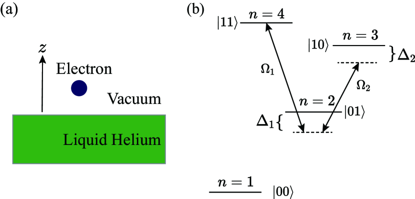
Figure 1: Schematic diagram of the CNOT gate based on SE. (a) The SE on the surface of liquid helium. (b) The two-qubit system is encoded in the four-level SE Rydberg states, where two coherent driving fields with frequencies $\omega_{j}$ and Rabi frequencies $\Omega_{j}$ ($j=1,2$) are applied simultaneously. Here, $\Delta_{1}$ and $\Delta_{2}$ are the single-photon and two-photon detunings, respectively.

As shown in Figure 1(a), along the direction $z$ perpendicular to the interface, the SE is attracted by the induced image charge inside the liquid helium and concurrently repulsed by the helium atoms, and therefore the motion of the SE is confined by the hydrogen-like potential $V=-\Lambda e^{2}/z$ for $z>0$, where $e$ is the charge of the electron and $\Lambda=(\epsilon-1)/[4(\epsilon+1)]$ with the dielectric constant $\epsilon\approx 1.057$. The quantized SE states possess the hydrogen-like energy spectrum as Platzman and Dykman (1999); Monarkha and Kono (2004)

$$\varepsilon_{n}^{(\perp)}=-\frac{m_{e}e^{4}\Lambda^{2}}{2\hbar^{2}n^{2}}=-\frac{R}{n^{2}},$$ (1)

where $m_{e}$ is the mass of the electron, the positive integer $n$ labels the SE state, and $R\approx 0.7$ meV Platzman and Dykman (1999) is the Rydberg energy. The wave function of SE is Nieto (2000)

$$\psi_{n}(z)=2n^{-5/2}r_{B}^{-3/2}z\exp\left(-\frac{z}{nr_{B}}\right)L_{n-1}^{(1)}\left(\frac{2z}{nr_{B}}\right),$$ (2)

where $r_{B}=\hbar^{2}/(m_{e}e^{2}\Lambda)$ is the effective Bohr radius, and

$$L_{n}^{(\alpha)}(x)=\frac{e^{x}x^{-\alpha}}{n!}\frac{d^{n}}{dx^{n}}(e^{-x}x^{n+\alpha})$$ (3)

is the Laguerre polynomial.

The expected positions $\langle z\rangle_{n}=\langle\psi_{n}|z|\psi_{n}\rangle$ of the electrons in different Rydberg states $|\psi_{n}\rangle$ are different. The electrons in higher excited states are further away from the liquid surface. For example, $\langle z\rangle_{2}/\langle z\rangle_{1}=4$, $\langle z\rangle_{3}/\langle z\rangle_{1}=9$, $\langle z\rangle_{4}/\langle z\rangle_{1}=16$ and so on. This phenomenon is remarkable for highly excited Rydberg states. The expected position $\langle z\rangle$ has practical applications in physical systems. For example, the electron with larger $\langle z\rangle$ has larger electric dipole moment and induces larger dipole-dipole interaction with the adjacent electrons, and thus can be used to couple adjacent electrons Jaksch et al. (2000); McDonnell et al. (2022). Meanwhile, in the gradient magnetic field, the electrons with different $\langle z\rangle$ have different spin-level shifts due to the Zeeman effect, and thus can be used to couple the Rydberg states with the spin states Tokura et al. (2006); Kawakami et al. (2023).

Encoding a two-qubit system on a single electron is analogous to the hyperentanglement which combines several DOFs of a single particle Barreiro et al. (2005); Yang et al. (2005); Deng et al. (2017). We consider the ground state and the first excited state of the SE as the “lower” mode and consider the highly excited Rydberg states as the “upper” mode. The first bit indicates which mode the SE is in. The “lower” mode is labeled as $|0\rangle$, and the “upper” mode is labeled as $|1\rangle$. Each mode comprises a two-level system, which is labeled by the second bit. Therefore, the ground state with $n=1$ is labeled as $|00\rangle$, the first excited state with $n=2$ is labeled as $|01\rangle$, the second excited state with $n=3$ is labeled as $|10\rangle$, and the third excited state with $n=4$ is labeled as $|11\rangle$, as shown in Figure 1(b). The CNOT gate in our scheme means that the second bit flips only if the state is in the “upper” mode, while the second bit doesn’t flip if the state is in the “lower” mode.

The level spacing of highly excited Rydberg states is narrow because the energy space $\Delta E_{n}$ decreases with $n$. Moreover, since the dipole moment matrix elements for the transitions between highly excited states are large, the direct transition between these states is sensitive to the frequency fluctuation of the driving fields Saffman et al. (2010). This sensitivity of the direct manipulation of highly excited states could easily cause the undesirable transition to other neighboring states. Therefore, we use the first excited state $|01\rangle$ as an intermediate state to realize the state swap between $|10\rangle$ and $|11\rangle$.

Because the first excited state $|01\rangle$ is the most dissipative state (see Appendix. A), we exploit the dark state in the EIT effect to reduce the population on $|01\rangle$. Two driving fields with frequencies $\omega_{1}$ ($\omega_{2}$) and Rabi frequencies $\Omega_{1}$ ($\Omega_{2}$) are used to drive the transition $|01\rangle\rightleftharpoons|11\rangle$ ($|01\rangle\rightleftharpoons|10\rangle$), as shown in Figure 1(b). The single-photon detuning is $\Delta_{1}=\omega_{1}-(\omega_{11}-\omega_{01})$ and the two-photon detuning is $\Delta_{2}=\omega_{1}-\omega_{2}-(\omega_{11}-\omega_{10})$, where $\omega_{01}$, $\omega_{10}$ and $\omega_{11}$ are the energies of the states $|01\rangle$, $|10\rangle$ and $|11\rangle$ respectively. As the driving frequencies are far detuned from the transitions between $|00\rangle$ and other states, we consider $|00\rangle$ to be a decoupled state. In the subspace spanned by $\{|01\rangle,|10\rangle,|11\rangle\}$, the Hamiltonian is

$$H=~{} \omega_{01}|01\rangle\langle 01|+\omega_{10}|10\rangle\langle 10|+\omega_{11}|11\rangle\langle 11|$$

$$-\Omega_{1}\cos\omega_{1}t(|01\rangle\langle 11|+|11\rangle\langle 01|)$$

$$-\Omega_{2}\cos\omega_{2}t(|01\rangle\langle 10|+|10\rangle\langle 01|),$$ (4)

where $\hbar=1$. In the rotating frame with driving frequencies $U=\exp[i\omega_{1}t|01\rangle\langle 01|+i(\omega_{1}-\omega_{2})t|10\rangle\langle 10|]$, under the rotating-wave approximation Scully and Zubairy (1997); Ai et al. (2010), and taking $\omega_{11}=0$ as the zero point of energy, the matrix form of the Hamiltonian reads

$$H_{I}=~{} i\frac{dU^{{\dagger}}}{dt}U+U^{{\dagger}}HU$$

$$=~{} -\frac{1}{2}\begin{pmatrix}-2\Delta_{1}&\Omega_{2}&\Omega_{1}\\ \Omega_{2}&-2\Delta_{2}&0\\ \Omega_{1}&0&0\end{pmatrix}.$$ (5)

The evolution of the system can be described by the quantum master equation Breuer and Petruccione (2002)

$$\frac{\partial}{\partial t}\rho=-i[H_{I},\rho]-\mathcal{L}(\rho),$$ (6)

where the Lindblad operator is

$$\mathcal{L}(\rho)=~{} \kappa_{1}[|01\rangle\langle 01|\rho|01\rangle\langle 01|-\frac{1}{2}\{|01\rangle\langle 01|,\rho\}]$$

$$+\kappa_{2}[|10\rangle\langle 10|\rho|10\rangle\langle 10|-\frac{1}{2}\{|10\rangle\langle 10|,\rho\}]$$

$$+\kappa_{3}[|11\rangle\langle 11|\rho|11\rangle\langle 11|-\frac{1}{2}\{|11\rangle\langle 11|,\rho\}]$$ (7)

with $\{A,B\}=AB+BA$ being the anti-commutator, and $\kappa_{1}$, $\kappa_{2}$ and $\kappa_{3}$ being the decay rates of the states $|01\rangle$, $|10\rangle$ and $|11\rangle$ respectively. In our scheme, the electron is only confined by the image potential and no electric holding field is applied. In this case, the decay rates of the Rydberg states of the SE decrease with $n$, cf. Appendix A. Thus, in the analytic calculation, we mainly consider the dissipations of the energy levels $|01\rangle$ and $|10\rangle$ and neglect the dissipation of $|11\rangle$, while all of the dissipations are considered in the numerical simulation. It is noteworthy that in experiments there is usually an electric holding field $E_{z}$ applied perpendicular to the liquid surface. For the experimental configuration such as $E_{z}\approx 200$ V/cm Kawakami et al. (2023) and $E_{z}\approx 1$ kV/cm Bradbury et al. (2011); Zou and Konstantinov (2022), the decay rates of the Rydberg states of the SE increase with $n$, cf. Appendix A. Recent works have provided efficient quantum algorithms to simulate the quantum open system both theoretically Zhang et al. (2021) and experimentally Wang et al. (2018b), even for the non-Markovian process Chen et al. (2022).

To solve the time evolution analytically, we neglect the quantum jump term and describe the evolution by the Schrödinger equation with the following non-Hermitian Hamiltonian

$$H_{I}^{d}=~{} H_{I}-i\frac{\kappa_{1}}{2}|01\rangle\langle 01|-i\frac{\kappa_{2}}{2}|10\rangle\langle 10|$$

$$=~{} -\frac{1}{2}\begin{pmatrix}-2\delta_{1}&\Omega_{2}&\Omega_{1}\\ \Omega_{2}&-2\delta_{2}&0\\ \Omega_{1}&0&0\end{pmatrix},$$ (8)

where $\delta_{1}=\Delta_{1}-i\kappa_{1}/2$, $\delta_{2}=\Delta_{2}-i\kappa_{2}/2$. When $\delta_{2}\ll\Omega_{1},\Omega_{2}$, we take $\delta_{2}$ as the perturbation term. The approximated eigenstates by taking $\delta_{2}=0$ are Fleischhauer et al. (2005)

$$\begin{split}&|a_{1}\rangle=-\sin\theta|10\rangle+\cos\theta|11\rangle,\\ &|a_{2}\rangle=\cos\phi|01\rangle+\cos\theta\sin\phi|10\rangle+\sin\theta\sin\phi|11\rangle,\\ &|a_{3}\rangle=-\sin\phi|01\rangle+\cos\theta\cos\phi|10\rangle+\sin\theta\cos\phi|11\rangle,\end{split}$$ (9)

where the mixing angles are $\tan\theta=\Omega_{1}/\Omega_{2}$ and $\tan 2\phi=\Omega/\delta_{1}$, and $\Omega=\sqrt{\Omega_{1}^{2}+\Omega_{2}^{2}}$. It is noteworthy that $|a_{1}\rangle$ is a dark state since there is no population on the state $|01\rangle$. As shown in Appendix B, the first-order approximations of the eigenvalues are

$$\begin{split}E_{1}\simeq&\frac{\Omega_{1}^{2}}{\Omega^{2}}\delta_{2},\\ E_{2}\simeq&\frac{\Omega}{2}+\frac{\delta_{1}}{2}+\frac{\Omega_{2}^{2}}{2\Omega^{2}}\delta_{2},\\ E_{3}\simeq&-\frac{\Omega}{2}+\frac{\delta_{1}}{2}+\frac{\Omega_{2}^{2}}{2\Omega^{2}}\delta_{2},\end{split}$$ (10)

The time evolution of the initial state $|\psi(0)\rangle=C_{1}|a_{1}\rangle+C_{2}|a_{2}\rangle+C_{3}|a_{3}\rangle$ is

$$|\psi(t)\rangle=~{} C_{1}e^{-iE_{1}t}|a_{1}\rangle+C_{2}e^{-iE_{2}t}|a_{2}\rangle+C_{3}e^{-iE_{3}t}|a_{3}\rangle$$

$$=~{} (C_{2}\cos\phi e^{-iE_{2}t}-C_{3}\sin\phi e^{-iE_{3}t})|01\rangle$$

$$+(-C_{1}\sin\theta e^{-iE_{1}t}+C_{2}\cos\theta\sin\phi e^{-iE_{2}t}$$

$$+C_{3}\cos\theta\cos\phi e^{-iE_{3}t})|10\rangle$$

$$+(C_{1}\cos\theta e^{-iE_{1}t}+C_{2}\sin\theta\sin\phi e^{-iE_{2}t}$$

$$+C_{3}\sin\theta\cos\phi e^{-iE_{3}t})|11\rangle.$$ (11)

The key point of the CNOT gate scheme is to swap the population of $|10\rangle$ and $|11\rangle$, while maintaining the low population of $|01\rangle$ in the final state. The state swapping is based on the population oscillation. As $E_{1}\ll E_{2},~{}E_{3}$, the main oscillation factors are $\exp(-iE_{2}t)$ and $\exp(-iE_{3}t)$. To achieve the maximum population reversal of $|10\rangle$ and $|11\rangle$, these two oscillation terms $\exp(-iE_{2}t)$ and $\exp(-iE_{3}t)$ should have the same period. The synchronization of $\exp(-iE_{2}t)$ and $\exp(-iE_{3}t)$ requires $E_{2}=-E_{3}$, so $\delta_{1}$ and $\delta_{2}$ must be much smaller than $\Omega$, i.e.,

$$\tan\phi=1.$$ (12)

Meanwhile, the oscillation term in the coefficient of $|10\rangle$ and $|11\rangle$ must be the same, which means that $\cos\theta=\sin\theta$, i.e.,

$$\Omega_{1}=\Omega_{2}.$$ (13)

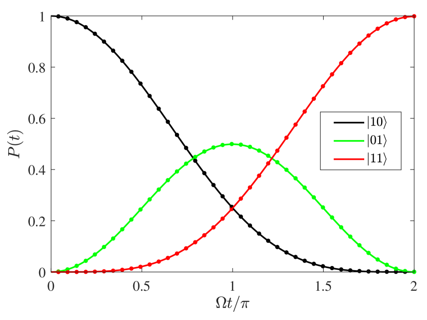
Figure 2: The populations $P(t)$ of different states with the initial state $|10\rangle$ and the dissipation rates $\kappa_{1}/\Omega=10^{-3}$, $\kappa_{2}=0.3439\kappa_{1}$ and $\kappa_{3}=0.1520\kappa_{1}$. The solid lines are the analytic solutions and the dots are the numerical solutions by the quantum master equation Eq. (7).

Under these conditions, if the initial state is $|\psi(0)\rangle=|10\rangle$, the final state is

$$|\psi(t)\rangle= \left(\frac{1}{2}\cos\frac{\Omega t}{2}e^{-i\frac{2\delta_{1}+\delta_{2}}{4}t}+\frac{1}{2}e^{-i\frac{\delta_{2}}{2}t}\right)|10\rangle$$

$$-\frac{i}{\sqrt{2}}\sin\frac{\Omega t}{2}e^{-i\frac{2\delta_{1}+\delta_{2}}{4}t}|01\rangle$$

$$+\left(\frac{1}{2}\cos\frac{\Omega t}{2}e^{-i\frac{2\delta_{1}+\delta_{2}}{4}t}-\frac{1}{2}e^{-i\frac{\delta_{2}}{2}t}\right)|11\rangle.$$ (14)

If the initial state $|\psi(0)\rangle=|01\rangle$, the final state is

$$|\psi(t)\rangle= -\frac{i}{\sqrt{2}}\sin\frac{\Omega t}{2}e^{-i\frac{2\delta_{1}+\delta_{2}}{4}t}|10\rangle$$

$$+\cos\frac{\Omega t}{2}e^{-i\frac{2\delta_{1}+\delta_{2}}{4}t}|01\rangle$$

$$-\frac{i}{\sqrt{2}}\sin\frac{\Omega t}{2}e^{-i\frac{2\delta_{1}+\delta_{2}}{4}t}|11\rangle.$$ (15)

If the initial state $|\psi(0)\rangle=|11\rangle$, the final state is

$$|\psi(t)\rangle= \left(\frac{1}{2}\cos\frac{\Omega t}{2}e^{-i\frac{2\delta_{1}+\delta_{2}}{4}t}-\frac{1}{2}e^{-i\frac{\delta_{2}}{2}t}\right)|10\rangle$$

$$-\frac{i}{\sqrt{2}}\sin\frac{\Omega t}{2}e^{-i\frac{2\delta_{1}+\delta_{2}}{4}t}|01\rangle$$

$$+\left(\frac{1}{2}\cos\frac{\Omega t}{2}e^{-i\frac{2\delta_{1}+\delta_{2}}{4}t}+\frac{1}{2}e^{-i\frac{\delta_{2}}{2}t}\right)|11\rangle.$$ (16)

The time evolution of different initial states is shown in Figure 2. The Rabi frequency $\Omega=10^{9}~{}\textrm{s}^{-1}$ Platzman and Dykman (1999) and the decay rate $\kappa_{1}=10^{6}~{}\textrm{s}^{-1}$ Monarkha and Sokolov (2007); Kawakami et al. (2021), thus $\kappa_{1}/\Omega=10^{-3}$. We take $\kappa_{2}=0.3439\kappa_{1}$ and $\kappa_{3}=0.1520\kappa_{1}$, according to Appendix A. The maximum population reversal between $|10\rangle$ and $|11\rangle$ is reached when $\Omega t=2\pi$. The analytical solutions are in good agreement with the numerical solutions calculated by Qutip Johansson et al. (2012, 2013).

III Fidelity analysis

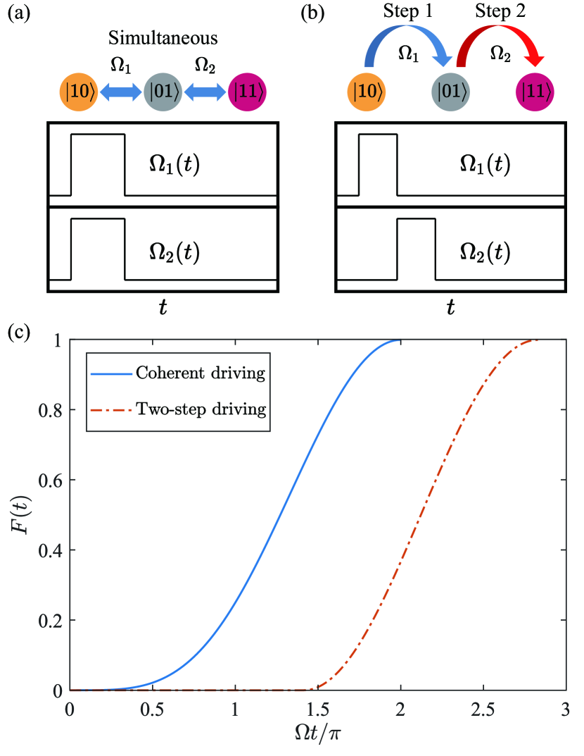
Figure 3: (a) Schematic diagram of the coherent-driving scheme. (b) Schematic diagram of the two-step driving scheme. (c) The fidelity $F$ of the state transfer $|10\rangle\to|11\rangle$. The dissipation rates are the same as Figure 2.

Since the driving frequencies are far detuned from the transition between $|00\rangle$ and other states, we consider $|00\rangle$ to be a decoupled state. From the time evolution in Eq. (14)-(16), the maximum population reversal between $|10\rangle$ and $|11\rangle$ is achieved when $\Omega t=2\pi$. The state fidelity $F$ between the final state $\rho(t)$ and the ideal target state $\rho_{i}$ is defined as Uhlmann (1976); Jozsa (1994)

$$F=\left(\textrm{Tr}\sqrt{\sqrt{\rho_{i}}\rho(t)\sqrt{\rho_{i}}}\right)^{2}.$$ (17)

In our coherent-driving scheme, two driving fields interact with the SE simultaneously, with the dark and bright states being used equally for the state transfer. The maximum fidelity is achieved when $t=2\pi/\Omega$, as shown in Figure 3(c). For comparison, we show the result of the two-step driving scheme in Figure 3(b). We derive the population reversal between $|10\rangle$ and $|01\rangle$ by the first driving pulse $\Omega_{1}(t)$, and then derive the population reversal between $|01\rangle$ and $|11\rangle$ by the second driving pulse $\Omega_{2}(t)$. The maximum fidelity is achieved when $t=2\sqrt{2}\pi/\Omega$, which is longer than the coherent-driving scheme. In addition, the two-step driving scheme can only achieve the one-way state transfer based on the driving pulse sequence, but a NOT-gate requires the bidirectional transfer with the same driving pulse sequence.

In Sec. II, we have found that $\Delta_{1}$ need to be much smaller than $\Omega$ in order to synchronize the oscillation terms $\exp(-iE_{2}t)$ and $\exp(-iE_{3}t)$. When the single-photon resonance condition is invalid, the fidelity of the state transfer decreases, as shown in Figure 4. It is noteworthy that the oscillation period changes with $\Delta_{1}$. Thus, the fidelity is calculated at the maximum in the first period. On the other hand, when $\Delta_{2}$ becomes large, the perturbation method is invalid, but the evolution of the states can still be derived from the master equation. As shown in Figure 4, when the two-photon resonance condition is invalid, the fidelity of the state transfer decreases because the EIT effect is suppressed.

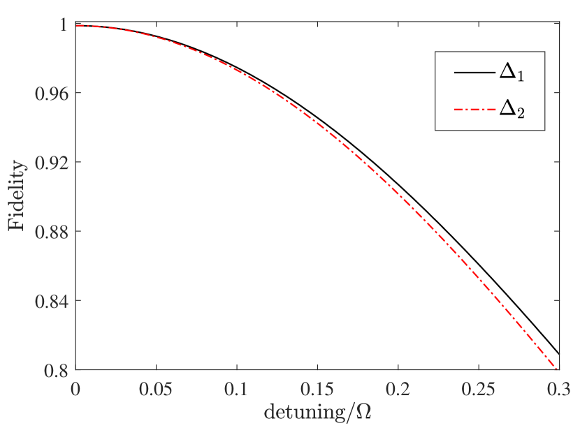
Figure 4: State fidelity versus the single-photon detuning $\Delta_{1}$ and the two-photon detuning $\Delta_{2}$. The dissipation rates are the same as Figure 2. The solid (solid-dot) line shows the dependence on $\Delta_{1}$ ($\Delta_{2}$) with $\Delta_{2}=0$ ($\Delta_{1}=0$).

Figure 3(c) only shows the fidelity of the state transfer with the input state $|10\rangle$. In Table 1 we present the output state fidelities of the CNOT gate under typical input states. When the control bit is $|0\rangle$, the target bit remains in the initial state. When the control bit is $|1\rangle$, the target bit flips. Meanwhile, when the input state is a superposition state, the output also corresponds to the characteristic of the CNOT gate. The output density matrices of $(|0\rangle+|1\rangle)\otimes|0\rangle/\sqrt{2}$ and $(|0\rangle+|1\rangle)\otimes|1\rangle/\sqrt{2}$ are shown in Figure 5.

Table 1: The output state fidelities of the CNOT gate under typical input states. The dissipation rates are the same as Figure 2.

Input state	Ideal output state	Fidelity
$|00\rangle$	$|00\rangle$	1
$|01\rangle$	$|01\rangle$	0.9987
$|10\rangle$	$|11\rangle$	0.9987
$|11\rangle$	$|10\rangle$	0.9987
$(|0\rangle+|1\rangle)\otimes|0\rangle/\sqrt{2}$	$(|00\rangle+|11\rangle)/\sqrt{2}$	0.9990
$(|0\rangle+|1\rangle)\otimes|1\rangle/\sqrt{2}$	$(|01\rangle+|10\rangle)/\sqrt{2}$	0.9980

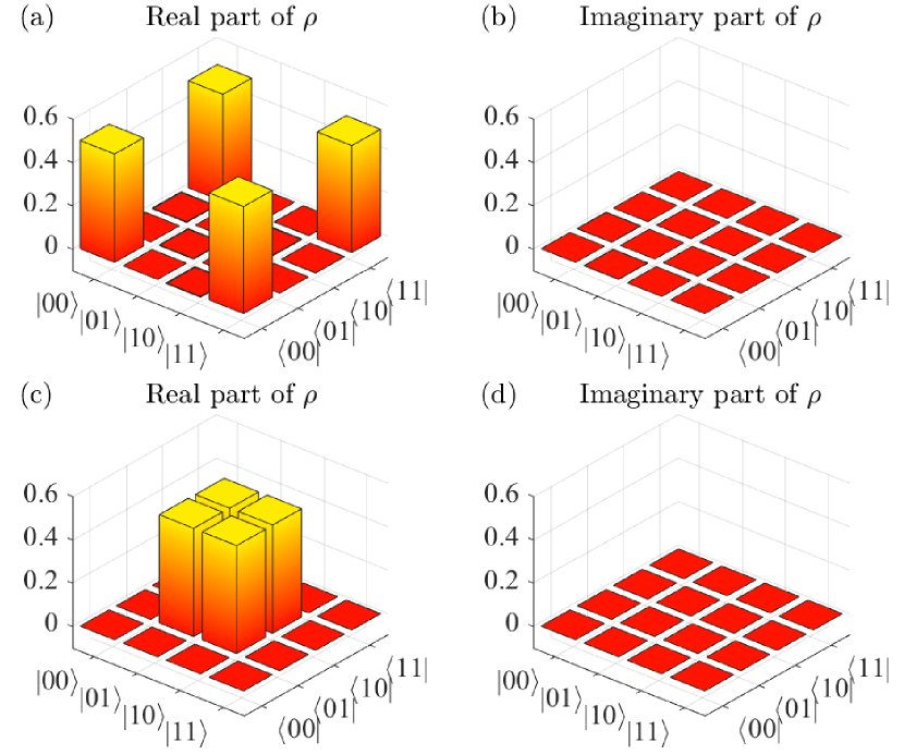
Figure 5: The matrix elements of the output density operator when the initial state is $(|0\rangle+|1\rangle)\otimes|0\rangle/\sqrt{2}$ for (a) and (b), and the initial state is $(|0\rangle+|1\rangle)\otimes|1\rangle/\sqrt{2}$ for (c) and (d). The dissipation rates are the same as Figure 2.

To demonstrate the characteristic of the entire gate, we calculate the gate fidelity which is defined as Palao and Kosloff (2002); Wu et al. (2017)

$$F=\frac{1}{N}|\textrm{Tr}(e^{i\phi}U_{r}^{{\dagger}})U_{i}|,$$ (18)

where $N$ is the dimension of the Hilbert space, $U_{i}$ is the ideal gate operation, $U_{r}$ is the real operation in our scheme, and $\phi$ is a global phase to maximize $F$. Since the transitions between $|00\rangle$ and other states are negligible, we can analytically derive the operation matrix of the CNOT gate in our scheme from the evolution of different initial states:

$$U_{r}= \begin{pmatrix}1&0&0&0\\ 0&a&0&0\\ 0&0&b&c\\ 0&0&c&b\end{pmatrix},$$ (19)

where

$$\begin{split}&a=e^{-\frac{(2\kappa_{1}+\kappa_{2})\pi}{4\Omega}},\\ &b=\frac{1}{2}e^{-\frac{(2\kappa_{1}+\kappa_{2})\pi}{4\Omega}}-\frac{1}{2}e^{-\frac{\kappa_{2}\pi}{2\Omega}},\\ &c=\frac{1}{2}e^{-\frac{(2\kappa_{1}+\kappa_{2})\pi}{4\Omega}}+\frac{1}{2}e^{-\frac{\kappa_{2}\pi}{2\Omega}}.\end{split}$$ (20)

This formula is obtained by an additional phase operation on $|01\rangle$, $|10\rangle$ and $|11\rangle$, which adds a $\pi$ phase to these three energy levels. Compared to the ideal CNOT gate

$$U_{i}= \begin{pmatrix}1&0&0&0\\ 0&1&0&0\\ 0&0&0&1\\ 0&0&1&0\end{pmatrix},$$ (21)

the fidelity of $U_{r}$ is

$$F=\frac{1}{4}|\textrm{Tr}(U_{r}^{T}U_{i})|=\frac{1+a}{4}+\frac{c}{2}.$$ (22)

Experimental systems usually apply a vertical static electric field $\vec{E}=E_{\perp}\vec{e}_{z}$ in order to tune the energy spacing between Rydberg states. The lifetime of the excited state decreases with $E_{\perp}$, and for typical $E_{\perp}=100$ V/cm it becomes 5 times shorter Monarkha and Sokolov (2007). Thus, in Figure 6 we analyze the gate fidelity under different dissipation rates. The fidelity $F>0.99$ in a wide range of $\kappa_{1}$, and $F=0.9989$ with parameters $\kappa_{1}/\Omega=10^{-3}$ which is experimentally achievable Platzman and Dykman (1999); Monarkha and Sokolov (2007); Kawakami et al. (2021).

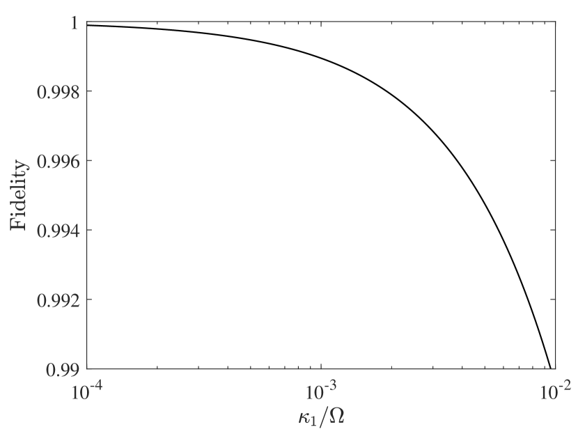
Figure 6: The gate fidelity between the ideal CNOT gate and the gate in our scheme under different dissipation rates.

IV Conclusion and remarks

In this work, we present a scheme to realize the CNOT gate in the four-level Rydberg structure of SE. We use a three-level structure to realize the state transfer. By applying two driving pulses simultaneously, we exploit the dark state in the EIT effect to suppress the population of the most-dissipative state and increase the robustness against dissipation Huang et al. (2022). We obtain the time evolution of the system both analytically and numerically. We optimize the Rabi frequencies and the detunings of the driving fields to achieve the maximum population exchange of $|10\rangle$ and $|11\rangle$. The optimal state transfer requires that both the single-photon and the two-photon resonances are satisfied. We also calculate the fidelity of the state transfer and of the entire gate. The fidelity is 0.9989 with experimentally achievable parameters.

The CNOT operation involves a three-level structure whose configuration can be the ladder type, $V$ type, or $\Lambda$-type Fleischhauer et al. (2005). The choice of configuration depends on the relative dissipation rates of the three levels. In our scheme, we mainly consider the case without the electric holding field. In this case the decay rates of the Rydberg states decrease with $n$. Therefore, we choose the $V$-type configuration to consider the most dissipative state as the intermediate state and use the EIT effect to suppress the population on this state. For the case with a considerable electric holding field, the decay rates are significantly different from those in the zero-field case, and the $\Lambda$-type configuration of the three-level structure should be chosen accordingly.

It’s noteworthy that both the iSWAP gate and CNOT gate can be used to construct universal quantum computation. The efficiencies of these two gates are determined by the character of the hardware. For example, in spin systems, it’s easier to realize the XY interaction by spin-spin interaction. Thus, the iSWAP gate is more efficient in this circumstance Lidar and Wu (2001); Schuch and Siewert (2003); Tanamoto et al. (2009). In our scheme we only use the dipole transition of the surface electron, and thus iSWAP gates do not have the advantage of CNOT gates. If the spin-spin interaction of surface electrons is used for quantum computation, the iSWAP gate may be a more efficient candidate.

In our scheme, the first logical bit of the two-bit system labels whether the electron is close or far away from the surface because the expected positions of different Rydberg states are different. The expected position $\langle z\rangle$ has practical applications in physical systems. Recent works have used the expected position of electrons to scale up the system. For example, the electron with larger $\langle z\rangle$ has larger electric dipole moment and induces larger dipole-dipole interaction with the adjacent electrons, and thus can be used to couple adjacent electrons Jaksch et al. (2000); McDonnell et al. (2022). Meanwhile, in the gradient magnetic field, the electrons with different $\langle z\rangle$ have different spin-level shifts due to the Zeeman effect, and thus can be used to couple the Rydberg states with the spin states Tokura et al. (2006); Kawakami et al. (2023). Our scheme demonstrates the advantages of precise manipulation on highly excited Rydberg states with narrow energy space and therefore provides potential applications in the schemes based on the dipole-dipole interaction of highly excited Rydberg states and the coupling between the Rydberg states and the spin states.

Appendix A Decay mechanism of the surface electron

The two-ripplon scattering in the short-wavelength range dominates the decay mechanism at low temperature, and the decay rate of the first excited state ($n=2$) is expressed as Monarkha and Sokolov (2006, 2007); Monarkha et al. (2010)

$$\frac{1}{\tau_{2,k}}=\frac{m_{e}\kappa_{0}^{2}}{4\pi\hbar\alpha\rho}\left(\frac{\rho}{4\hbar^{2}\alpha}\right)^{1/3}\left(\frac{\partial V}{\partial z}\right)_{11}\left(\frac{\partial V}{\partial z}\right)_{22}\Delta_{21}^{2/3},$$ (23)

where $V(z)$ is the electron potential, $\kappa_{0}$ is the penetration depth of the electron wave function into liquid, $\alpha$ is the surface tension of liquid helium, and $\rho$ is the liquid mass density. The decay rate is determined by the diagonal matrix element of $\partial V/\partial z$ and the energy difference $\Delta$ between the initial state and the lower-lying Rydberg states that the initial state leaks to.

Since the spontaneous two-ripplon emission process decreases the energy of surface electrons, we neglect the leakage to the higher-lying Rydberg states when calculating the decay rate. The decay rate of the highly-excited Rydberg state is the sum of the leakage to all lower-lying Rydberg states, i.e., the decay rate $\kappa^{(n)}$ of the Rydberg state with the quantum number $n$ is

$$\kappa^{(n)}=K\sum_{l=1}^{n-1}\left(\frac{\partial V}{\partial z}\right)_{ll}\left(\frac{\partial V}{\partial z}\right)_{nn}\Delta_{nl}^{2/3},$$ (24)

where $K=\frac{m_{e}\kappa_{0}^{2}}{4\pi\hbar\alpha\rho}(\frac{\rho}{4\hbar^{2}\alpha})^{1/3}$ is a constant.

Table 2: The decay rates of five lowest excited states under the electric holding field. Note that the dependence of $\kappa^{(n)}$ on $n$ is significantly different for the case with and without the applied electric field.

$E_{z}$ (V/cm)	$\kappa^{(3)}/\kappa^{(2)}$	$\kappa^{(4)}/\kappa^{(2)}$	$\kappa^{(5)}/\kappa^{(2)}$	$\kappa^{(6)}/\kappa^{(2)}$
0	0.3439	0.1520	0.0795	0.0465
100	0.9807	1.0050	1.0442	1.0890
200	1.1260	1.2418	1.3552	1.4663
500	1.3233	1.5950	1.8487	2.0927
1000	1.4701	1.8800	2.2689	2.6477

When there is no electric holding field, $V(z)=-\Lambda e^{2}/z$ is the image potential. The decay rates can be calculated from the energy spectrum (1) and the wave function (2). As shown in the first row of Table 2, the decay rate decreases with increasing $n$. This is because highly-excited states are further away from the surface. Since ripplons represent the height variations of the helium surface, the couplings between the highly-excited electrons and ripplons are weak.

In experiments, there is usually an electric holding field $E_{z}$ applied perpendicular to the liquid surface. By considering $E_{z}$ as an uniform field, the corresponding potential can be expressed as $eE_{z}z$. As shown in the lower four rows of Table 2, the decay rates of the excited states under different electric holding fields are calculated from the eigen values and wave functions, which are solved numerically. The energy level spacings between higher-laying Rydberg states enlarge with increasing $E_{z}$. Meanwhile, the SE in the holding field is closer to the liquid surface than that without the holding field, especially for the highly-excited states. Thus, for the experimental configuration with a considerable electric holding field, the decay rates are significantly different from the zero-field case according to Eq. (24).

Appendix B Eigenvalues from the perturbation method

Assuming that $E_{n}=-x/2$, the secular equation of Eq. (8) is

$$x[x^{2}+2(\delta_{1}+\delta_{2})x+4\delta_{1}\delta_{2}-\Omega^{2}]-2\Omega_{1}^{2}\delta_{2}=0,$$ (25)

where $\Omega=\sqrt{\Omega_{1}^{2}+\Omega_{2}^{2}}$. To solve the secular equation, we assume $\delta_{2}$ as a perturbation term and

$$x_{j}\approx x_{0j}+A_{j}\delta_{2}.$$ (26)

The zero-order terms satisfies

$$x_{0j}[x_{0j}^{2}+2(\delta_{1}+\delta_{2})x_{0j}+4\delta_{1}\delta_{2}-\Omega^{2}]=0,$$ (27)

and the solutions are

$$\begin{split}x_{01}&=0,\\ x_{02}&=-\delta_{1}-\delta_{2}-\sqrt{(\delta_{1}-\delta_{2})^{2}+\Omega^{2}}\\ &\simeq-\delta_{1}-\delta_{2}-\Omega-\frac{\delta_{1}-\delta_{2}}{2\Omega}(\delta_{1}-\delta_{2})\\ &\simeq-\delta_{1}-\delta_{2}-\Omega,\\ x_{03}&=-\delta_{1}-\delta_{2}+\sqrt{(\delta_{1}-\delta_{2})^{2}+\Omega^{2}}\\ &\simeq-\delta_{1}-\delta_{2}+\Omega+\frac{\delta_{1}-\delta_{2}}{2\Omega}(\delta_{1}-\delta_{2})\\ &\simeq-\delta_{1}-\delta_{2}+\Omega.\end{split}$$ (28)

The approximation is valid when $\delta_{1},\delta_{2}\ll\Omega$. Thus, the secular equation is transformed into

$$(x-x_{01})(x-x_{02})(x-x_{03})-2\Omega_{1}^{2}\delta_{2}=0.$$ (29)

Inserting $x_{j}\approx x_{0j}+A_{j}\delta_{2}$, we can obtain

$$\begin{split}A_{1}&=\frac{2\Omega_{1}^{2}}{(x_{01}-x_{02})(x_{01}-x_{03})}\simeq-\frac{2\Omega_{1}^{2}}{\Omega^{2}},\\ A_{2}&=\frac{2\Omega_{1}^{2}}{(x_{02}-x_{01})(x_{02}-x_{03})}\simeq\frac{\Omega_{1}^{2}}{\Omega^{2}},\\ A_{3}&=\frac{2\Omega_{1}^{2}}{(x_{03}-x_{01})(x_{03}-x_{02})}\simeq\frac{\Omega_{1}^{2}}{\Omega^{2}},\end{split}$$ (30)

and the eigenvalues to the first-order approximation as

$$\begin{split}E_{1}&\simeq\frac{\Omega_{1}^{2}}{\Omega^{2}}\delta_{2},\\ E_{2}&\simeq\frac{\Omega}{2}+\frac{\delta_{1}}{2}+\frac{\Omega_{2}^{2}}{2\Omega^{2}}\delta_{2},\\ E_{3}&\simeq-\frac{\Omega}{2}+\frac{\delta_{1}}{2}+\frac{\Omega_{2}^{2}}{2\Omega^{2}}\delta_{2}.\end{split}$$ (31)

References

- Barenco et al. (1995) A. Barenco, C. H. Bennett, R. Cleve, D. P. DiVincenzo, N. Margolus, P. Shor, T. Sleator, J. A. Smolin, and H. Weinfurter, Phys. Rev. A 52, 3457 (1995).
- Sleator and Weinfurter (1995) T. Sleator and H. Weinfurter, Phys. Rev. Lett. 74, 4087 (1995).
- Chitambar and Gour (2019) E. Chitambar and G. Gour, Rev. Mod. Phys. 91, 025001 (2019).
- Buluta and Nori (2009) I. Buluta and F. Nori, Science 326, 108 (2009).
- Weimer et al. (2010) H. Weimer, M. Müller, I. Lesanovsky, P. Zoller, and H. P. Büchler, Nat. Phys. 6, 382 (2010).
- Georgescu et al. (2014) I. M. Georgescu, S. Ashhab, and F. Nori, Rev. Mod. Phys. 86, 153 (2014).
- Mostame and Schützhold (2008) S. Mostame and R. Schützhold, Phys. Rev. Lett. 101, 220501 (2008).
- Buluta et al. (2011) I. Buluta, S. Ashhab, and F. Nori, Rep. Prog. Phys. 74, 104401 (2011).
- Xiang et al. (2013) Z. L. Xiang, S. Ashhab, J. Q. You, and F. Nori, Rev. Mod. Phys. 85, 623 (2013).
- Zhang et al. (2017) J. Zhang, Y. X. Liu, R. B. Wu, K. Jacobs, and F. Nori, Phys. Rep. 679, 1 (2017).
- Frisk Kockum et al. (2019) A. Frisk Kockum, A. Miranowicz, S. De Liberato, S. Savasta, and F. Nori, Nat. Rev. Phys. 1, 19 (2019).
- Makhlin et al. (2001) Y. Makhlin, G. Schön, and A. Shnirman, Rev. Mod. Phys. 73, 357 (2001).
- Yamamoto et al. (2003) T. Yamamoto, Y. A. Pashkin, O. Astafiev, Y. Nakamura, and J. S. Tsai, Nature 425, 941 (2003).
- Liu et al. (2005) Y. X. Liu, J. Q. You, L. F. Wei, C. P. Sun, and F. Nori, Phys. Rev. Lett. 95, 087001 (2005).
- You and Nori (2005) J. Q. You and F. Nori, Phys. Today 58, 42 (2005).
- You and Nori (2011) J. Q. You and F. Nori, Nature 474, 589 (2011).
- Gu et al. (2017) X. Gu, A. F. Kockum, A. Miranowicz, Y. X. Liu, and F. Nori, Phys. Rep. 718, 1 (2017).
- Jones et al. (1998) J. A. Jones, M. Mosca, and R. H. Hansen, Nature 393, 344 (1998).
- Feng et al. (2013) G. R. Feng, G. F. Xu, and G. L. Long, Phys. Rev. Lett. 110, 190501 (2013).
- Turchette et al. (1995) Q. A. Turchette, C. J. Hood, W. Lange, H. Mabuchi, and H. J. Kimble, Phys. Rev. Lett. 75, 4710 (1995).
- Rauschenbeutel et al. (1999) A. Rauschenbeutel, G. Nogues, S. Osnaghi, P. Bertet, M. Brune, J. M. Raimond, and S. Haroche, Phys. Rev. Lett. 83, 5166 (1999).
- Walther et al. (2006) H. Walther, B. T. Varcoe, B.-G. Englert, and T. Becker, Rep. Prog. Phys. 69, 1325 (2006).
- Burkard et al. (2020) G. Burkard, M. J. Gullans, X. Mi, and J. R. Petta, Nat. Rev. Phys. 2, 129 (2020).
- Chiorescu et al. (2004) I. Chiorescu, P. Bertet, K. Semba, Y. Nakamura, C. J. P. M. Harmans, and J. E. Mooij, Nature 431, 159 (2004).
- DiCarlo et al. (2009) L. DiCarlo, J. M. Chow, J. M. Gambetta, L. S. Bishop, B. R. Johnson, D. I. Schuster, J. Majer, A. Blais, L. Frunzio, S. M. Girvin, and R. J. Schoelkopf, Nature 460, 240 (2009).
- Scarlino et al. (2019) P. Scarlino, D. J. van Woerkom, A. Stockklauser, J. V. Koski, M. C. Collodo, S. Gasparinetti, C. Reichl, W. Wegscheider, T. Ihn, K. Ensslin, and A. Wallraff, Phys. Rev. Lett. 122, 206802 (2019).
- Cirac and Zoller (1995) J. I. Cirac and P. Zoller, Phys. Rev. Lett. 74, 4091 (1995).
- Poyatos et al. (1998) J. F. Poyatos, J. I. Cirac, and P. Zoller, Phys. Rev. Lett. 81, 1322 (1998).
- Figgatt et al. (2019) C. Figgatt, A. Ostrander, N. M. Linke, K. A. Landsman, D. Zhu, D. Maslov, and C. Monroe, Nature 572, 368 (2019).
- Li et al. (2003) X. Q. Li, Y. W. Wu, D. Steel, D. Gammon, T. H. Stievater, D. S. Katzer, D. Park, C. Piermarocchi, and L. J. Sham, Science 301, 809 (2003).
- Ciriano-Tejel et al. (2021) V. N. Ciriano-Tejel, M. A. Fogarty, S. Schaal, L. Hutin, B. Bertrand, L. Ibberson, M. F. Gonzalez-Zalba, J. Li, Y.-M. Niquet, M. Vinet, and J. J. L. Morton, PRX Quantum 2, 010353 (2021).
- Jelezko et al. (2004) F. Jelezko, T. Gaebel, I. Popa, M. Domhan, A. Gruber, and J. Wrachtrup, Phys. Rev. Lett. 93, 130501 (2004).
- Wei and Deng (2013) H. R. Wei and F. G. Deng, Phys. Rev. A 88, 042323 (2013).
- Zhang et al. (2020) J. F. Zhang, S. S. Hegde, and D. Suter, Phys. Rev. Lett. 125, 030501 (2020).
- Fleischhauer et al. (2005) M. Fleischhauer, A. Imamoglu, and J. P. Marangos, Rev. Mod. Phys. 77, 633 (2005).
- Liu et al. (2014) Y. X. Liu, X. W. Xu, A. Miranowicz, and F. Nori, Phys. Rev. A 89, 043818 (2014).
- Liu et al. (2016) Q. C. Liu, T. F. Li, X. Q. Luo, H. Zhao, W. Xiong, Y. S. Zhang, Z. Chen, J. S. Liu, W. Chen, F. Nori, J. S. Tsai, and J. Q. You, Phys. Rev. A 93, 053838 (2016).
- Gu et al. (2016) X. Gu, S. N. Huai, F. Nori, and Y. X. Liu, Phys. Rev. A 93, 063827 (2016).
- Wang et al. (2018a) X. Wang, A. Miranowicz, H. R. Li, F. L. Li, and F. Nori, Phys. Rev. A 98, 023821 (2018a).
- Wang and Clerk (2012) Y. D. Wang and A. A. Clerk, Phys. Rev. Lett. 108, 153603 (2012).
- McDonnell et al. (2022) K. McDonnell, L. F. Keary, and J. D. Pritchard, Phys. Rev. Lett. 129, 200501 (2022).
- Peng et al. (2014) B. Peng, Ş. K. Özdemir, W. Chen, F. Nori, and L. Yang, Nat. Commun. 5, 5082 (2014).
- Platzman and Dykman (1999) P. M. Platzman and M. I. Dykman, Science 284, 1967 (1999).
- Kawakami et al. (2021) E. Kawakami, A. Elarabi, and D. Konstantinov, Phys. Rev. Lett. 126, 106802 (2021).
- Koolstra et al. (2019) G. Koolstra, G. Yang, and D. I. Schuster, Nat. Commun. 10, 5323 (2019).
- Kawakami et al. (2019) E. Kawakami, A. Elarabi, and D. Konstantinov, Phys. Rev. Lett. 123, 086801 (2019).
- Schuster et al. (2010) D. I. Schuster, A. Fragner, M. I. Dykman, S. A. Lyon, and R. J. Schoelkopf, Phys. Rev. Lett. 105, 040503 (2010).
- Kawakami et al. (2023) E. Kawakami, J. Chen, M. Benito, and D. Konstantinov, arXiv (2023), 2303.03688 .
- Lyon (2006) S. A. Lyon, Phys. Rev. A 74, 052338 (2006).
- Zhou et al. (2022) X. J. Zhou, G. Koolstra, X. F. Zhang, G. Yang, X. Han, B. Dizdar, X. H. Li, R. Divan, W. Guo, K. W. Murch, D. I. Schuster, and D. F. Jin, Nature 605, 46 (2022).
- Glasson et al. (2001) P. Glasson, V. Dotsenko, P. Fozooni, M. J. Lea, W. Bailey, G. Papageorgiou, S. E. Andresen, and A. Kristensen, Phys. Rev. Lett. 87, 176802 (2001).
- Ikegami et al. (2009) H. Ikegami, H. Akimoto, and K. Kono, Phys. Rev. Lett. 102, 046807 (2009).
- Rees et al. (2011) D. G. Rees, I. Kuroda, C. A. Marrache-Kikuchi, M. Höfer, P. Leiderer, and K. Kono, Phys. Rev. Lett. 106, 026803 (2011).
- Ikegami et al. (2012) H. Ikegami, H. Akimoto, D. G. Rees, and K. Kono, Phys. Rev. Lett. 109, 236802 (2012).
- Rees et al. (2016a) D. G. Rees, N. R. Beysengulov, J. J. Lin, and K. Kono, Phys. Rev. Lett. 116, 206801 (2016a).
- Rees et al. (2016b) D. G. Rees, N. R. Beysengulov, Y. Teranishi, C. S. Tsao, S. S. Yeh, S. P. Chiu, Y. H. Lin, D. A. Tayurskii, J. J. Lin, and K. Kono, Phys. Rev. B 94, 045139 (2016b).
- Badrutdinov et al. (2020) A. O. Badrutdinov, D. G. Rees, J. Y. Lin, A. V. Smorodin, and D. Konstantinov, Phys. Rev. Lett. 124, 126803 (2020).
- Zou and Konstantinov (2022) S. Zou and D. Konstantinov, New J. Phys. 24, 103026 (2022).
- Bradbury et al. (2011) F. R. Bradbury, M. Takita, T. M. Gurrieri, K. J. Wilkel, K. Eng, M. S. Carroll, and S. A. Lyon, Phys. Rev. Lett. 107, 266803 (2011).
- Kielpinski et al. (2002) D. Kielpinski, C. Monroe, and D. J. Wineland, Nature 417, 709 (2002).
- Gallagher (1994) T. F. Gallagher, Rydberg Atoms (Cambridge University Press, 1994).
- Saffman et al. (2010) M. Saffman, T. G. Walker, and K. Mølmer, Rev. Mod. Phys. 82, 2313 (2010).
- Monarkha and Sokolov (2006) Y. P. Monarkha and S. S. Sokolov, Low Temp. Phys. 32, 970 (2006).
- Monarkha and Sokolov (2007) Y. P. Monarkha and Sokolov, J. Low Temp. Phys. 148, 157 (2007).
- Monarkha et al. (2010) Y. P. Monarkha, S. S. Sokolov, A. V. Smorodin, and N. Studart, Low Temp. Phys. 36, 565 (2010).
- Barreiro et al. (2005) J. T. Barreiro, N. K. Langford, N. A. Peters, and P. G. Kwiat, Phys. Rev. Lett. 95, 260501 (2005).
- Yang et al. (2005) T. Yang, Q. Zhang, J. Zhang, J. Yin, Z. Zhao, M. Żukowski, Z.-B. Chen, and J.-W. Pan, Phys. Rev. Lett. 95, 240406 (2005).
- Deng et al. (2017) F. G. Deng, B. C. Ren, and X. H. Li, Sci. Bull. 62, 46 (2017).
- Jaksch et al. (2000) D. Jaksch, J. I. Cirac, P. Zoller, S. L. Rolston, R. Côté, and M. D. Lukin, Phys. Rev. Lett. 85, 2208 (2000).
- Tokura et al. (2006) Y. Tokura, W. G. van der Wiel, T. Obata, and S. Tarucha, Phys. Rev. Lett. 96, 047202 (2006).
- Wang et al. (2018b) B. X. Wang, M. J. Tao, Q. Ai, T. Xin, N. Lambert, D. Ruan, Y. C. Cheng, F. Nori, F. G. Deng, and G. L. Long, npj Quantum Inf. 4, 52 (2018b).
- Wang et al. (2018c) Y. Y. Wang, J. Qiu, Y. Q. Chu, M. Zhang, J. M. Cai, Q. Ai, and F. G. Deng, Phys. Rev. A 97, 042313 (2018c).
- Monarkha and Kono (2004) Y. Monarkha and K. Kono, Two-Dimensional Coulomb Liquids and Solids (Springer Science & Business Media, 2004).
- Nieto (2000) M. M. Nieto, Phys. Rev. A 61, 034901 (2000).
- Scully and Zubairy (1997) M. O. Scully and M. S. Zubairy, Quantum Optics (Cambridge University Press, 1997).
- Ai et al. (2010) Q. Ai, Y. Li, H. Zheng, and C. P. Sun, Phys. Rev. A 81, 042116 (2010).
- Breuer and Petruccione (2002) H. P. Breuer and F. Petruccione, The Theory of Open Quantum Systems (Oxford University Press, 2002).
- Zhang et al. (2021) N. N. Zhang, M. J. Tao, W. T. He, X. Y. Chen, X. Y. Kong, F. G. Deng, N. Lambert, and Q. Ai, Front. Phys. 16, 51501 (2021).
- Chen et al. (2022) X. Y. Chen, N. N. Zhang, W. T. He, X. Y. Kong, M. J. Tao, F. G. Deng, Q. Ai, and G. L. Long, npj Quantum Inf. 8, 22 (2022).
- Johansson et al. (2012) J. R. Johansson, P. D. Nation, and F. Nori, Comput. Phys. Commun. 183, 1760 (2012).
- Johansson et al. (2013) J. R. Johansson, P. D. Nation, and F. Nori, Comput. Phys. Commun. 184, 1234 (2013).
- Uhlmann (1976) A. Uhlmann, Rep. Math. Phys. 9, 273 (1976).
- Jozsa (1994) R. Jozsa, J. Mod. Opt. 41, 2315 (1994).
- Palao and Kosloff (2002) J. P. Palao and R. Kosloff, Phys. Rev. Lett. 89, 188301 (2002).
- Wu et al. (2017) C. Z. Wu, B. Qi, C. L. Chen, and D. Y. Dong, IEEE Trans. Cybern. 47, 4405 (2017).
- Huang et al. (2022) H. B. Huang, J. J. Lin, Y. X. Yao, K. Y. Xia, Z. Q. Yin, and Q. Ai, Ann. Phys. (Berlin) 534, 2200157 (2022).
- Lidar and Wu (2001) D. A. Lidar and L. A. Wu, Phys. Rev. Lett. 88, 017905 (2001).
- Schuch and Siewert (2003) N. Schuch and J. Siewert, Phys. Rev. A 67, 032301 (2003).
- Tanamoto et al. (2009) T. Tanamoto, Y. X. Liu, X. D. Hu, and F. Nori, Phys. Rev. Lett. 102, 100501 (2009).