Interpretable Ensembles of Hyper-Rectangles as Base Models

Abstract

A new extremely simple ensemble-based model with the uniformly generated axis-parallel hyper-rectangles as base models (HRBM) is proposed. Two types of HRBMs are studied: closed rectangles and corners. The main idea behind HRBM is to consider and count training examples inside and outside each rectangle. It is proposed to incorporate HRBMs into the gradient boosting machine (GBM). Despite simplicity of HRBMs, it turns out that these simple base models allow us to construct effective ensemble-based models and avoid overfitting. A simple method for calculating optimal regularization parameters of the ensemble-based model, which can be modified in the explicit way at each iteration of GBM, is considered. Moreover, a new regularization called the ”step height penalty” is studied in addition to the standard L1 and L2 regularizations. An extremely simple approach to the proposed ensemble-based model prediction interpretation by using the well-known method SHAP is proposed. It is shown that GBM with HRBM can be regarded as a model extending a set of interpretable models for explaining black-box models. Numerical experiments with real datasets illustrate the proposed GBM with HRBMs for regression and classification problems. Experiments also illustrate computational efficiency of the proposed SHAP modifications. The code of proposed algorithms implementing GBM with HRBM is publicly available.

Keywords: gradient boosting machine, SHAP, ensemble-based models, explainability, rectangles

1 Introduction

Despite the rapid development of various approaches in machine learning, the ensemble-based methodology remains one of the most effective approaches for solving the regression and classification problems. Therefore, ensemble models have been extensively studied in the machine learning community, and a huge amount of methods for solving machine learning problems, including classification and regression, have been developed in recent years [1, 2, 3, 4, 5, 6, 7, 8, 9, 10]. These methods are based on training a set of weak or base models from data such that their predictions are combined in some way to obtain a strong classifier or a regressor with a more accurate and generalizable result.

Two largest groups of ensemble-based methods can be pointed out. The first group (bagging) consists of methods [11] which are based on constructing base models on subsets of training data. One of the best-known bagging models is the Random Forest (RF) [12], which uses a large number of randomly built individual decision trees, each trained on data sets generated by means of bootstrap sampling. Another effective bagging model is the Extremely Randomized Trees (ERTs), which is proposed by Geurts et al. [13]. In contrast to RFs, the ERT algorithm at each node chooses a split point randomly for each feature and then selects the best split among these features.

The second group (boosting) consists of methods based on a sequential and dependent process. Well-known boosting models are AdaBoost [14], the gradient boosting machines (GBMs) [15, 16] and its modifications XGBoost [17], LightGBM [18], CatBoost [19]. The main idea behind the gradient boosting methods is to sequentially build each base model on the gradient descent direction of a loss function, based on differences between the true values of target variables and predicted values obtained from previous base models for all training examples. Gradient boosting is typically used with decision trees as base learners. Decision trees in gradient boosting provide accurate results in reasonable computation time. Moreover, it is pointed out by Natekin and Knoll [20] that small trees in many practical results provide better results, and there is much evidence that even complex models with rich tree structure provide almost no benefit over compact trees. The assumption of weak learners typically holds, and they can eventually generate a perfect fit. In particular, a special case of a decision tree with only one split (a tree stump) can be also successfully used in gradient boosting [21]. Besides decision trees, other base-learner models can be incorporated into gradient boosting [22], including linear models [23], p-splines [24], Markov random fields [25], wavelets [26].

In many applications, base models for boosting should be as simple as possible to avoid overfitting caused by the greedy structure of algorithms. Following the idea to simplify the base models, we propose an extremely simple model that can be incorporated into a GBM as a base model for solving different machine learning problems. The proposed model is called the Hyper-Rectangle as the Base Model (HRBM). It is represented as a closed axis-parallel rectangle or an axis-parallel rectangle corner. The main idea behind HRBM is to consider and count training examples inside and outside each rectangle. From this point of view, the base models become to be very simple. Rectangles are randomly generated at each iteration of GBM, and the best rectangle among the generated ones is used as the base model at the corresponding iteration. The best rectangle is determined in accordance with a goal to cover at least one training point. As a result, a single rectangle is used at each iteration of GBM. In spite of simplicity of HRBMs, it turns out that these simple base models allow us to construct effective ensemble-based models and avoid overfitting. GBM with HRBMs is denoted as GBM-HRBM below.

An important property of HRBMs is that the corresponding ensemble-based models can be simply interpreted by means of the interpretation method called SHapley Additive exPlanations (SHAP) [27, 28], which is inspired by game-theoretic Shapley values [29]. SHAP has an important shortcoming: its computational complexity depends on the number of features and cannot be applied to models having data of the high dimension without some approximation. Surprisingly, boosting models with HRBM have a very simple interpretation in terms of SHAP. This is really an interesting result. Moreover, GBM-HRBM due to its simple interpretation can be regarded as an interpretable meta-model approximating a complex black-box model.

Two types of HRBMs are studied. The first one is based on uniformly generated closed hyper-rectangles which have certain bounds. The second type is based on uniformly generated corners.

Our contributions can be summarized as follows:

1. A new extremely simple ensemble-based model with axis-parallel hyper-rectangles or corners as base models is proposed.

2. It is shown how HRBM incorporated into GBM. Simple expressions are derived for searching optimal parameters of HRBMs at each iteration of the boosting model and for computing the GBM-HRBM predictions.

3. A way for calculation of optimal regularization parameters of the ensemble-based model is considered. The optimal regularization parameters can simply be computed and modified at each iteration of GBM-HRBM. Moreover, a new regularization called the “step height penalty” in addition to the standard $L_{1}$ and $L_{2}$ regularizations is proposed.

4. The problem of the GBM-HRBM prediction interpretation by using the well-known method SHAP is solved in a computationally simple way. In fact, two modifications of SHAP are proposed, which solves the interpretation problem in a short time in comparison with using the original SHAP. The modifications are called the model-based SHAP and the data-based SHAP. In accordance with the first modification, the calculated Shapley values depend solely on the model but non on the data whereas the second modification depends on the data.

5. Numerical experiments with well-known real datasets illustrate the proposed GBM-HRBM for regression and classification problems. The experiments also compare two types of the rectangle models: closed rectangles and corners. Moreover, experiments with modifications of SHAP illustrate their computational efficiency. The corresponding code implementing GBM-HRBM is publicly available at: https://github.com/andruekonst/HRBM

The paper is organized as follows. Related work can be found in Section 2. A formal definition of HRBM is given in Section 3. Section 4 consider in detail how HRBMs can be incorporated into GBM. Questions of regularization and its optimal parameters are studied in Section 5. Algorithms of training and testing GBM-HRBM are considered in Section 6. Modifications of SHAP for interpretation predictions provided by ensemble-based models with HRBMs are proposed in Section 7. Numerical experiments are provided in Section 8. Concluding remarks can be found in Section 9. Appendix contains proofs of propositions.

2 Related work

Ensemble-based models, GBM. Ensemble-based methods can be regarded as a powerful approach to improve predictive performance and robustness of machine learning models. A detailed consideration of various types of ensemble-based models can be found in Zhou’s book [10]. Exhaustive descriptions of many ensemble approaches are presented in various survey papers, for instance, in [3, 30, 31, 6, 32, 8, 9]. Most authors assert that GBM [15, 16] and its modifications, including XGBoost [17], LightGBM [18], CatBoost [19], can be viewed as the best-known ensemble-based models.

Comprehensive surveys of GBMs and their comparison with other methods can be found in [33, 34, 35, 36]. Many modifications of GBMs use decision trees as one of the most accurate base models in GBMs [37, 20]. The same can be said about ERTs [38]. However, our study shows that HRBM as the base model can lead to better models from the computation and accuracy points of view.

Interpretation methods. Many methods have been developed to explain black-box models. The first well-known method is the Local Interpretable Model-agnostic Explanations (LIME) [39]. The main idea behind the method is to approximate predictions of a black-box model by a linear function of features. Due to success of LIME, various its modifications have been also proposed [40, 41, 42, 43, 44].

Another explanation method is the SHAP [27, 28]. It is based on applying a game-theoretic approach and Shapley values [29]. Broeck et al. [45] studied general questions of the SHAP computational efficiency. Various modifications of SHAP have been developed to explain different machine learning models and tools [46, 47, 48, 49, 50, 51, 52]. Applications of SHAP can be found in [53, 54, 55], Approaches to reduce the computational complexity of SHAP were also proposed in [56, 57, 58, 59, 60]. Many interpretation methods and their comparison were considered and studied in survey papers [61, 62, 63, 64, 65, 66, 67, 68] in detail.

Several interpretation approaches have been developed to efficiently explain predictions of GBM by using SHAP [69, 70, 71, 72, 73, 74, 75, 76]. However, the proposed HRBMs incorporated into GBM make SHAP computationally very simple by high-dimensional data.

3 Formal definition of HRBM

We introduce HRBM that can be incorporated into GBM as well as other ensemble models as a base model for solving various machine learning problems.

Given $N$ training data (examples) $S=\{(\mathbf{x}_{1},y_{1}),...,(\mathbf{x}_{N},y_{N})\}$, in which each vector $\mathbf{x}_{i}=(x_{i}^{(1)},...,x_{i}^{(d)})$ may belong to an arbitrary set $\mathcal{X}$ and represents a feature vector involving $d$ features, $y_{i}\in\mathcal{Y}=\{1,...,C\}$ represents the class of the associated examples in the classification task or $y_{i}\in\mathcal{Y}\subset\mathbb{R}$ represents the observed outputs in the regression task. Machine learning aims to construct a classifier or a regression model $f(\mathbf{x})$ that minimizes the expected risk $\mathbb{E}_{(X.Y)\sim p(\mathbf{x},y)}\left[l(Y,f(X))\right]$, where $p(\mathbf{x},y)$ is a joint density, and $l:\mathcal{Y}\times\mathcal{X}\rightarrow\mathbb{R}_{+}$ is a loss function.

Let $\mathbf{r}$ be a $d$-dimensional rectangle defined in the Cartesian space $\mathbb{R}^{d}$ as

$$\mathbf{r}=\prod_{j=1}^{d}[a^{(j)},b^{(j)}],$$ (1)

where $\mathbf{a}=(a^{(1)},...,a^{(d)})$ and $\mathbf{b}=(b^{(1)},...,b^{(d)})$ are two vectors such that $a^{(j)}\leq b^{(j)}$ for all $j=1,...,d$, which form the $d$-dimensional rectangle or hyper-rectangle.

Then HRBM is a piecewise-constant function with two distinct values: inside and outside the rectangle. It can be represented as:

$$A(\mathbf{x};\mathbf{r},v_{in},v_{out})=\mathbb{I}[\mathbf{x}\in\mathbf{r}](v_{in}-v_{out})+v_{out},$$ (2)

where $v_{in}$ and $v_{out}$ are values inside and outside the rectangle which are defined below; $\mathbb{I}[\mathbf{x}\in\mathbf{r}]$ is the indicator function taking value $1$ if $\mathbf{x}\in\mathbf{r}$, and value $0$ if $\mathbf{x}\notin\mathbf{r}$.

It follows from (2) that function $A$ takes two values: $A(\mathbf{x};\mathbf{r},v_{in},v_{out})=v_{in}$ if point $\mathbf{x}$ belongs to rectangle $\mathbf{r}$, and $A(\mathbf{x};\mathbf{r},v_{in},v_{out})=v_{out}$, if $\mathbf{x}$ does not belong to $\mathbf{r}$.

Given a rectangle $\mathbf{r}$, values $v_{in}$ and $v_{out}$ can be found by solving the following optimization problems:

$$v_{in}=\arg\min_{v}\sum_{i=1}^{N}l(y_{i},v)\cdot\mathbb{I}[\mathbf{x}_{i}\in\mathbf{r}],$$ (3)

$$v_{out}=\arg\min_{v}\sum_{i=1}^{N}l(y_{i},v)\cdot\mathbb{I}[\mathbf{x}_{i}\notin\mathbf{r}].$$ (4)

Here $l(y_{i},v)$ is a loss function which penalizes the distance between $y_{i}$ and $v$. It can be seen from (3) and (4) that value $v_{in}$ is nothing else but a simple prediction obtained on all training points which fall into rectangle $\mathbf{r}$. For example, if we take the regression loss $l(y_{i},v)=(y_{i}-v)^{2}$, then $v_{in}$ is the mean value of observed outputs corresponding to $\mathbf{x}_{i}$ inside $\mathbf{r}$. The same can be said about $v_{out}$ which is determined similarly, but using all points $\mathbf{x}_{i}$ outside $\mathbf{r}$.

It is important to point out that values of $v_{out}$ can be replaced with the bias term which is pre-calculated for the whole dataset as follows:

$$q=\arg\min_{q}\sum_{i=1}^{N}l(y_{i},q).$$ (5)

Hence, $v_{out}$ is computed as $v_{out}=q-v_{in}$. On the one hand, this representation of rectangles is more effective from the computational point of view because the bias $q$ is computed without analyzing whether points $\mathbf{x}_{i}$ belong to a rectangle. On the other hand, we use the first representation with $v_{in}$ and $v_{out}$ to simplify consideration of the rectangle properties.

There are different types of rectangles which define their generation. We consider the following two types:

1. Closed rectangles: when all elements of vectors $\mathbf{a}$ and $\mathbf{b}$ are finite. In this case, we can write

   $$\mathbf{x}\in\mathbf{r}\iff\bigwedge_{j=1}^{d}\left(x^{(j)}\in[a^{(j)},b^{(j)}]\right).$$ (6)

   The rectangle can also be defined by taking its center $\mathbf{c}=(c^{(1)},...,c^{(d)})$ and its width vector $\mathbf{w}=\mathbf{b}-\mathbf{a}$.

2. Corners of rectangles: when some elements of vectors $\mathbf{a}$ or $\mathbf{b}$ are unrestricted. In this case, we have a corner of the rectangle. It can be defined by the corner center $\mathbf{c}$ and conditions $a^{(j)}\rightarrow-\infty$ or $b^{(j)}\rightarrow\infty$.

We also will denote the $j$-th rectangle feature (the edge) as $r^{(j)}=[a^{(j)},b^{(j)}]$.

It follows from the above introduced HRBM that it is a very simple model which can be used as a base model in ensemble-based models. Therefore, we consider how HRBM can be efficiently incorporated into ensembles, in particular, into GBM.

4 Ensembles of HRBMs

Inherently, HRBM is an extremely simple model, and thus cannot approximate complex functions. However, ensembles of such models are much more expressive, but only in a case when the base models are dependent. Indeed, consider a set of independent HRBM models $A_{1}(\mathbf{x}),\dots,A_{k}(\mathbf{x})$. In case of the mean squared loss function, values inside and outside each rectangle are calculated as averages of target values for training points which fall into the corresponding rectangle. By averaging the ensemble predictions, we get for an example $\mathbf{x}$:

$$A(\mathbf{x})=\frac{1}{k}\sum_{i=1}^{k}A_{i}(\mathbf{x})=\frac{1}{k}\sum_{i=1}^{k}(v_{out}^{(i)}+\mathbb{I}[\mathbf{x}\in\mathbf{r}_{i}](v_{in}^{(i)}-v_{out}^{(i)}))\approx\overline{y},$$ (7)

which is close to constant $\overline{y}$.

Indeed, let us express $v_{out}^{(i)}$ through $q-v_{in}^{(i)}$. Then

$$A(\mathbf{x}) =\frac{1}{k}\sum_{i=1}^{k}(q-v_{in}^{(i)}-\mathbb{I}[\mathbf{x}\in\mathbf{r}_{i}]q)$$

$$=q\left(1-\frac{k_{in}}{k}\right)-\frac{1}{k}\sum_{i=1}^{k}v_{in}^{(i)}$$ (8)

where $k_{in}=\sum_{i=1}^{k}\mathbb{I}[\mathbf{x}\in\mathbf{r}_{i}]$.

Note that $v_{in}^{(i)}$ under condition of the mean squared loss function can be regarded as a mean $\overline{y}_{i}$ of target values corresponding to points which fall into the $i$-th rectangle. If rectangles are independent and random, then they correspond to bootstrapping that uses random sampling with replacement. Hence, we can write

$$A(\mathbf{x})=q\left(1-\frac{k_{in}}{k}\right)-\widetilde{y}=\overline{y}=\mathrm{const},$$ (9)

where $\widetilde{y}$ is the mean of the bootstrap sample.

Taking into account the above, we propose to use GBM which makes rectangles dependent.

Below we use $\mathbb{I}_{in}^{(i)}$ and $\mathbb{I}_{out}^{(i)}$ as abridged notations of $\mathbb{I}[\mathbf{x}_{i}\in\mathbf{r}]$ and $\mathbb{I}[\mathbf{x}_{i}\notin\mathbf{r}]$, respectively.

4.1 HRBM in Gradient Boosting

Let us consider GBM [16] which can be regarded as an ensemble method with dependent base models. The main idea behind GBM is to sequentially build each base model on the gradient descent direction of a loss function, based on the residual (the difference between predicted value and the true value of each example) from previous models [20]. In other words, GBM iteratively improves predictions $F_{i}(\mathbf{x})$ of $y$ for $\mathbf{x}$ with respect to the so-called residual approximation loss function by adding new base learners $f_{i}(\mathbf{x})\in\mathcal{F}$ that improve upon the previous ones, forming an additive ensemble model of size $T$:

$$F_{0}(\mathbf{x})=\overline{y},\ \ F_{i}(\mathbf{x})=F_{i-1}(\mathbf{x})+\gamma f_{i}(\mathbf{x}),\ i=1,...,T,$$ (10)

where $\gamma$ is a learning rate; $\mathcal{F}$ is a set of base learners, for instance, the set of decision trees; $\overline{y}$ is the mean target value over the whole dataset, which is regarded as an initialization of boosting.

The algorithm aims to minimize a loss function $l$, for instance, the squared error $L_{2}$-loss, by iteratively computing the gradient in accordance with the standard gradient descent method. A single base model implementing function $f_{i}$, for example, the decision tree, is constructed at each iteration to fit the negative gradients. It is trained on a new dataset $\{(\mathbf{x}_{j},\rho_{j}^{(i)})\}$, where $\rho_{j}^{(i)}$, $j=1,...,N$, are residuals defined as partial derivatives of the expected loss function at each point $\mathbf{x}_{j}$.

We propose to use HRBM as a base model in GBM, i.e., we take

$$f_{k}(\mathbf{x})=A(\mathbf{x};\theta_{k}),$$ (11)

where the parameter vector $\theta_{k}$ is defined as

$$\theta_{k}=(\mathbf{r}_{k},v_{in},v_{out}).$$ (12)

The parameter vector $\theta_{k}$ is chosen to optimize some functional. The first approach for implementing that is to approximate the negative residuals:

$$\rho_{i}^{(k)}=\left.-\frac{\partial l(y_{i},z)}{\partial z}\right|_{z=F_{k-1}(\mathbf{x}_{i})}.$$ (13)

Hence, we can write

$$\theta_{k}=\arg\min_{\theta_{k}}\sum_{i=1}^{N}\hat{l}\left(A(\mathbf{x}_{i};\theta_{k}),\rho_{i}^{(k)}\right),$$ (14)

where $\hat{l}$ is the residual approximation loss function.

A more advanced approach is based on applying the second derivatives of the loss function. Let us denote the first order derivatives as $g_{i}$:

$$g_{i}=\left.\frac{\partial l(y_{i},z)}{\partial z}\right|_{z=F_{k-1}(\mathbf{x}_{i})},$$ (15)

and the second order derivatives as $h_{i}$:

$$h_{i}=\left.\frac{\partial^{2}l(y_{i},z)}{\partial z^{2}}\right|_{z=F_{k-1}(\mathbf{x}_{i})}.$$ (16)

It should be noted that $g_{i}$ and $h_{i}$ depend on $\mathbf{x}_{i}$ as well as on the number $k$ of iteration. However, we omit the iteration index for brevity because $v_{in}$ and $v_{out}$ are determined through $g_{i}$ and $h_{i}$ for each iteration.

Note that we set $\gamma$ equal to $1$ when we build $f_{k}$, i.e., when we are searching for optimal values $v_{in}$ and $v_{out}$ in order to further reduce the absolute value of HRBM by multiplying by $\gamma$. The loss function can be expanded as follows:

$$l(y_{i},F_{k}(\mathbf{x}_{i}))=l(y_{i},F_{k-1}(\mathbf{x}_{i}))+g_{i}\cdot f_{k}(\mathbf{x}_{i})+\frac{1}{2}h_{i}(f_{k}(\mathbf{x}_{i}))^{2}+o((f_{k}(\mathbf{x}_{i}))^{2}),$$ (17)

so the empirical loss minimization is equivalent to the following optimization problem:

$$\frac{1}{N}\sum_{i=1}^{N}\left(g_{i}\cdot f_{k}(\mathbf{x}_{i})+\frac{1}{2}h_{i}(f_{k}(\mathbf{x}_{i}))^{2}+o((f_{k}(\mathbf{x}_{i}))^{2})\right)\rightarrow\min.$$ (18)

In case of small values $f_{k}(\mathbf{x}_{i})$, the optimization problem can be approximately rewritten as follows:

$$\hat{L}=\frac{1}{N}\sum_{i=1}^{N}\left(g_{i}\cdot f_{k}(\mathbf{x}_{i})+\frac{1}{2}h_{i}(f_{k}(\mathbf{x}_{i}))^{2}\right)\rightarrow\min.$$ (19)

We have two different base algorithms. If we would not know function $f$, i.e., we have a model-agnostic gradient boosting, then problem (19) leads to residuals of form:

$$\rho_{i}=-\frac{g_{i}}{h_{i}}.$$ (20)

The optimal HRBM values can be found in this case as follows:

$$\begin{cases}v_{in}=-\frac{1}{\sum_{i=1}^{N}\mathbb{I}_{in}^{(i)}}\sum_{i=1}^{N}\mathbb{I}_{in}^{(i)}\cdot\dfrac{g_{i}}{h_{i}},\\ v_{out}=-\frac{1}{\sum_{i=1}^{N}\mathbb{I}_{out}^{(i)}}\sum_{i=1}^{N}\mathbb{I}_{out}^{(i)}\cdot\dfrac{g_{i}}{h_{i}}.\end{cases}$$ (21)

Since the base model is HRBM, then a more precise solution can be obtained. First, for the sake of brevity, we define the function $f_{k}(\mathbf{x}_{i})$ for the $k$-th current iteration as:

$$f_{k}(\mathbf{x}_{i})=\mathbb{I}_{in}^{(i)}v_{in}+\mathbb{I}_{out}^{(i)}v_{out}.$$ (22)

Let us denote also for brevity:

$$G_{in}=\sum_{i=1}^{N}\mathbb{I}_{in}^{(i)}\cdot g_{i},\ G_{out}=\sum_{i=1}^{N}\mathbb{I}_{out}^{(i)}\cdot g_{i},$$ (23)

$$H_{in}=\sum_{i=1}^{N}\mathbb{I}_{in}^{(i)}\cdot h_{i},\ H_{out}=\sum_{i=1}^{N}\mathbb{I}_{out}^{(i)}\cdot h_{i}.$$ (24)

The loss function (19) has a minimum at a point with zero derivatives, namely:

$$\dfrac{\partial\hat{L}}{\partial v_{in}}=\dfrac{1}{N}\left(G_{in}+H_{in}\cdot v_{in}\right)=0,$$ (25)

$$\dfrac{\partial\hat{L}}{\partial v_{out}}=\dfrac{1}{N}\left(G_{out}+H_{out}\cdot v_{out}\right)=0.$$ (26)

It follows from the above that optimal values of $v_{in}$ and $v_{out}$ can be calculated from the following simple expressions:

$$v_{in}=-\frac{G_{in}}{H_{in}},\ v_{out}=-\frac{G_{out}}{H_{out}}.$$ (27)

Optimal values of $v_{in}$ and $v_{out}$ obtained by using (21) and (27) are different in general. For the loss functions with a constant second derivative, such as mean squared error, the values (21) and (27) are the same, but, for more complex functions, such as the cross-entropy, solution (27) is more accurate. In addition, the second solution, in contrast to the classical gradient boosting, allows us to introduce regularization on the model values $v_{in}$ and $v_{out}$.

If we multiply the base functions by the learning rate $\gamma$, then the result only indirectly control the model smoothness and has different effect which depend on absolute values of the loss function gradient. At that, values $v_{in}$ and $v_{out}$ are of the form:

$$v_{in}=-\gamma\frac{G_{in}}{H_{in}},\ v_{out}=-\gamma\frac{G_{out}}{H_{out}}.$$ (28)

A rectangle is a weak model, but if it is trained on a small number of training sample points, then the model may also lead to overfitting. In addition, noise in the target variable also has a significant effect on increase of the error. To overcome these difficulties, the gradient boosting algorithm can be improved by estimating the accuracy of base models on a validation set. To implement that, a base model is built based on the training set at each iteration. Then it is verified whether it does not reduce the accuracy on the validation set. Finally, if the validation is successful, then values $v_{in}$ and $v_{out}$ are recalculated on the entire training set. In this case, the division into training and validation sets can be performed once as well as at each iteration.

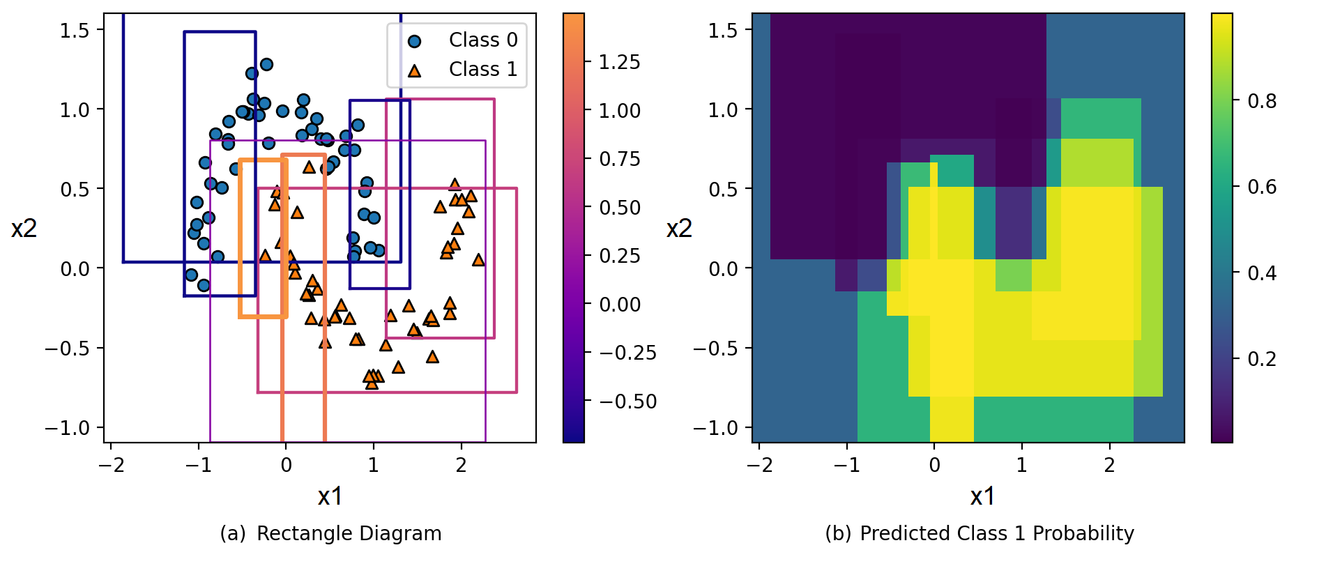
Figure 1: An illustrative example of HRBMs in the form of rectangles in classification on the two moons dataset: (a) generated rectangles after $8$ iterations; (b) predicted probabilities of Class 1 obtained by using GBM-HRBM with $8$ iterations

An illustrative classification example using the well-known “two moons” dataset is depicted in Fig. 1. Fig. 1 (a) shows closed rectangles generated at each iteration of GBM-HRBM. Colors and thickness of the rectangle lines correspond to $v_{in}$ for each rectangle, whose values are logits of the class 1. For clarity, the model contains only 8 rectangles. The loss function in this case is a binary cross entropy applied to the sigmoid $\sigma$ from the gradient boosting output:

$$l(y,z)=y\cdot\ln(\sigma(z))+(1-y)\cdot\ln(1-\sigma(z)).$$ (29)

Fig. 1 (b) shows predicted probabilities of Class 1 obtained by using GBM-HRBM after $8$ iterations with $8$ rectangles shown in Fig. 1 (a).

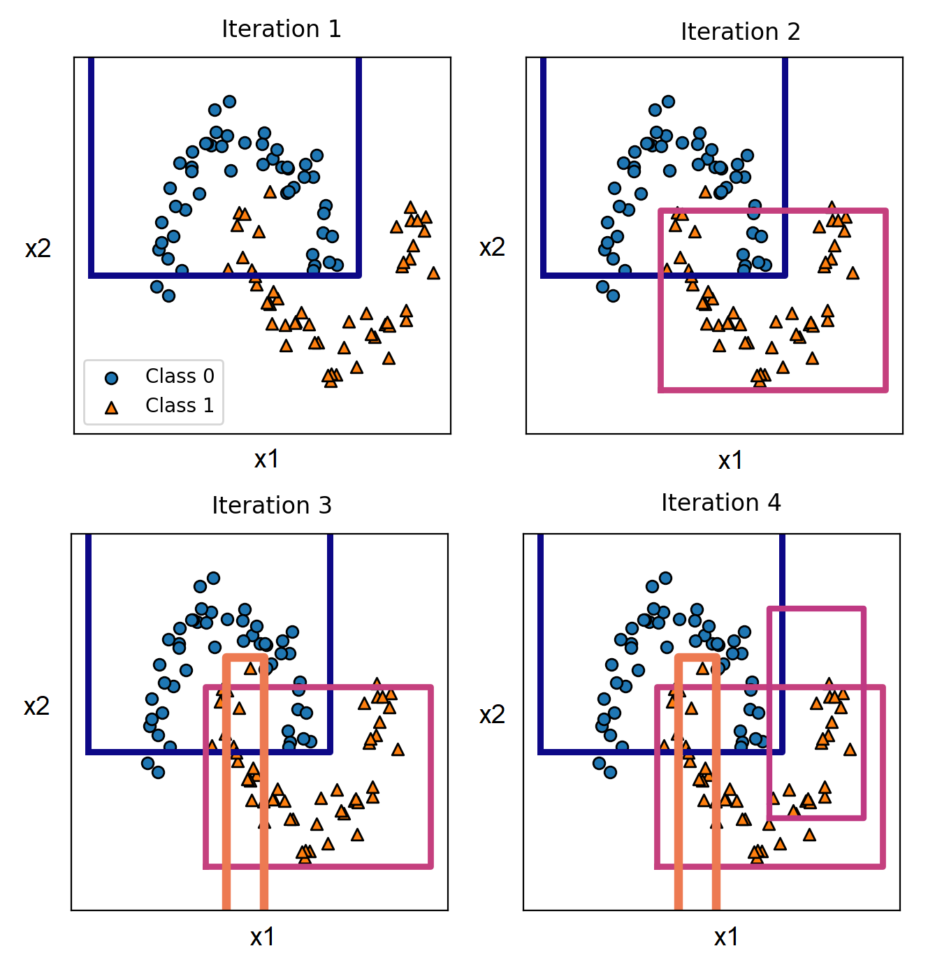
Figure 2: Rectangles generated at four iterations for classification

Fig. 2 illustrates how the rectangles are generated at each iteration. We show only four iterations. It can be seen from Fig. 2 that rectangles are generated to cover the data domain.

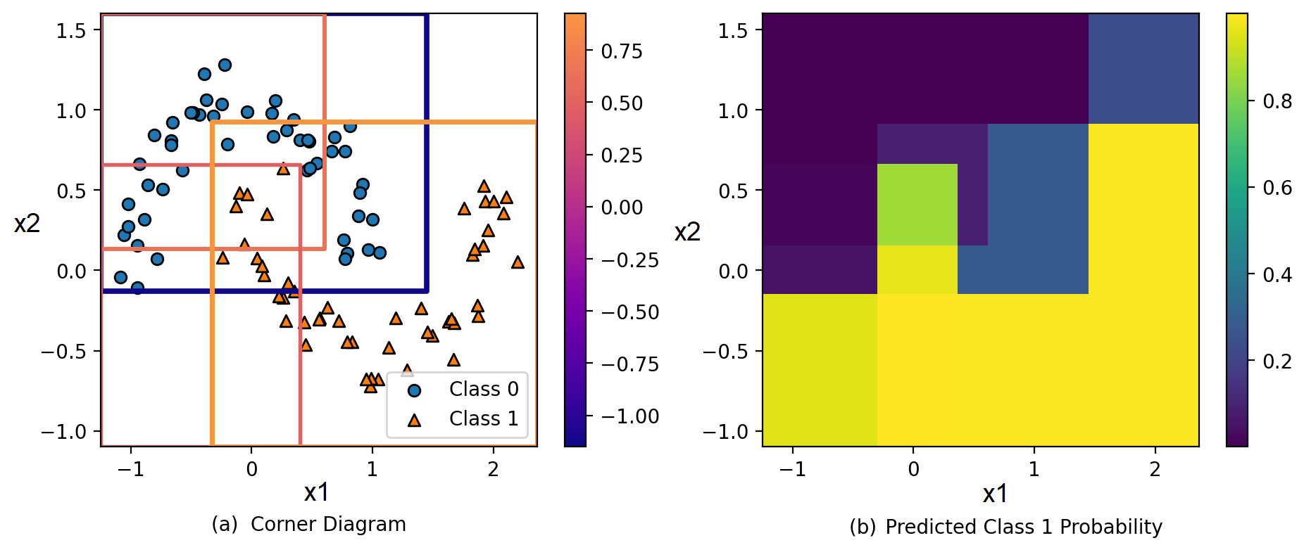
Figure 3: An illustrative example of HRBMs in the form of corners in classification on the two moons dataset: (a) generated rectangles after $4$ iterations; (b) predicted probabilities of Class 1 obtained by using GBM-HRBM with $4$ iterations

Fig. 3 is similar to Fig. 1, but it illustrates classification example using $4$ generated corners instead of $8$ rectangles. In particular, Fig. 3 (a) shows $4$ corners generated during $4$ iterations of GBM-HRBM. Fig. 3 (b) shows predicted probabilities of Class 1 obtained by using GBM-HRBM after $4$ iterations with $4$ corners shown in Fig. 3 (a). We see that the predicted probabilities are more uncertain in comparison with the case of rectangles shown in Fig. 1 (b). However, it does not mean that corners provide worse results. We take only four corners (compare with eight rectangles in the example in Fig. 1) in order to make pictures with corners visible. Fig. 4 illustrates how the corners are generated at each iteration. We again show only four iterations of GBM-HRBM.

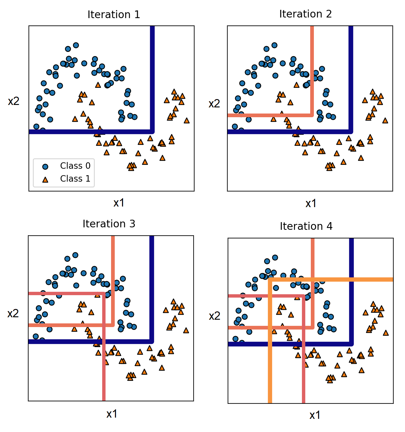
Figure 4: Corners generated at four iterations for classification

Fig. 5 illustrates an one-dimensional regression task implemented by using GBM-HRBM with $5$ iterations ($5$ rectangles). Rectangles in this case are represented by segments. Points (small circles) of the training set, the unknown truth function (the dashed line), and rectangles (segments) are depicted in Fig. 5 (a). Each segment is located at a height which is equal to the inside value $v_{in}$ of the corresponding rectangle. Bias $q$ is depicted by the dash-and-dot line. Fig. 5 (b) illustrates predictions obtained by using GBM-HRBM with 5 iterations. It can be seen from Fig. 5 (b) that even five iterations allow us to get accurate approximation of the unknown truth function. Fig. 6 illustrates how rectangles in the regression task are added at each iteration of GBM-HRBM. It can be seen from Fig. 6 (Iteration 1) that the first rectangle ($f_{1}$ in Fig. 5 (a)) divides all points into two subsets: (1) points $\mathbf{x}$ which fall inside the corresponding segment $[0,0.5]$; (2) points which fall outside the segment $[0.5,1]$. The second iteration generates the rectangle $[0.4,0.92]$ ($f_{2}$ in Fig. 5 (a)). Its intersection with the first segment forms additional subsets of points. It is interesting to see that rectangles after the second iteration approximate the unknown function. The same process of adding rectangles is depicted in other pictures of Fig. 6.

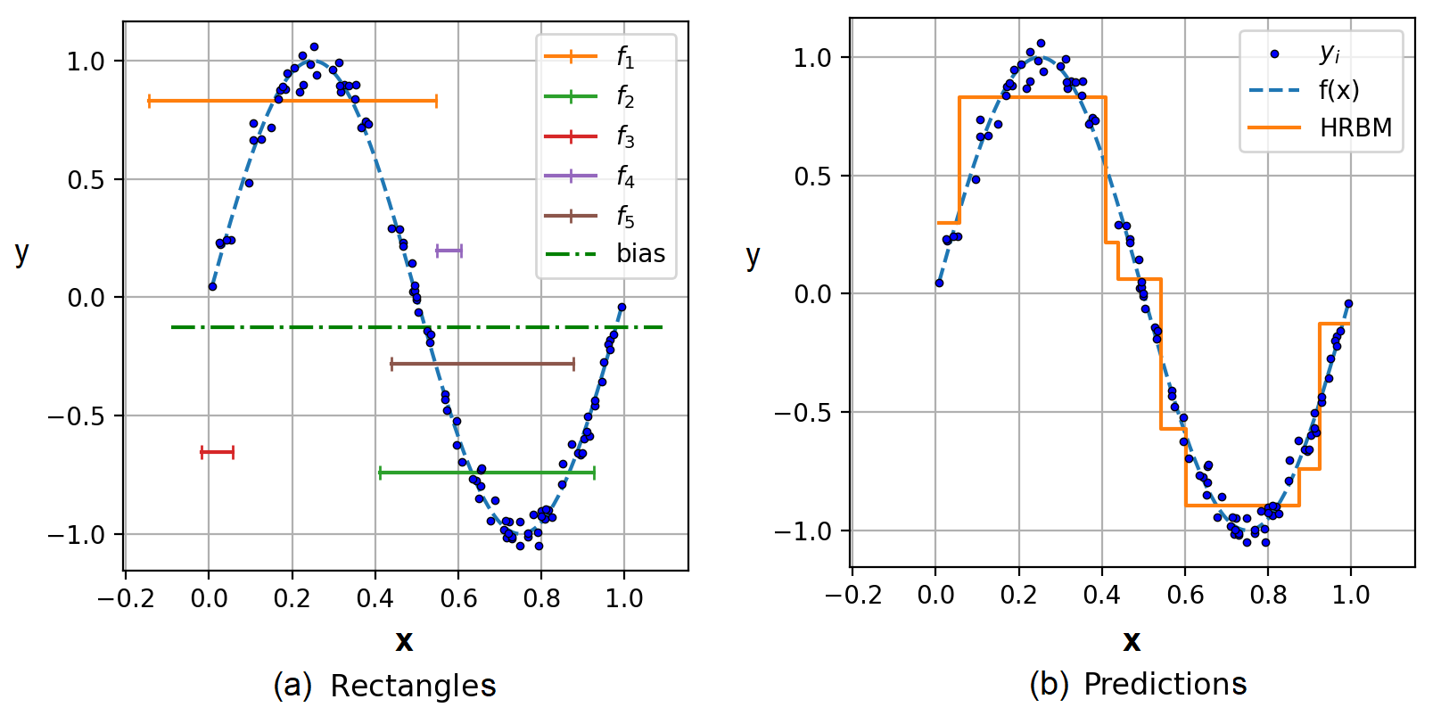
Figure 5: An illustrative example of HRBMs in regression: (a) generated one-dimensional rectangles after $5$ iterations; (b) predictedregression values obtained by using GBM-HRBM with $5$ iterations

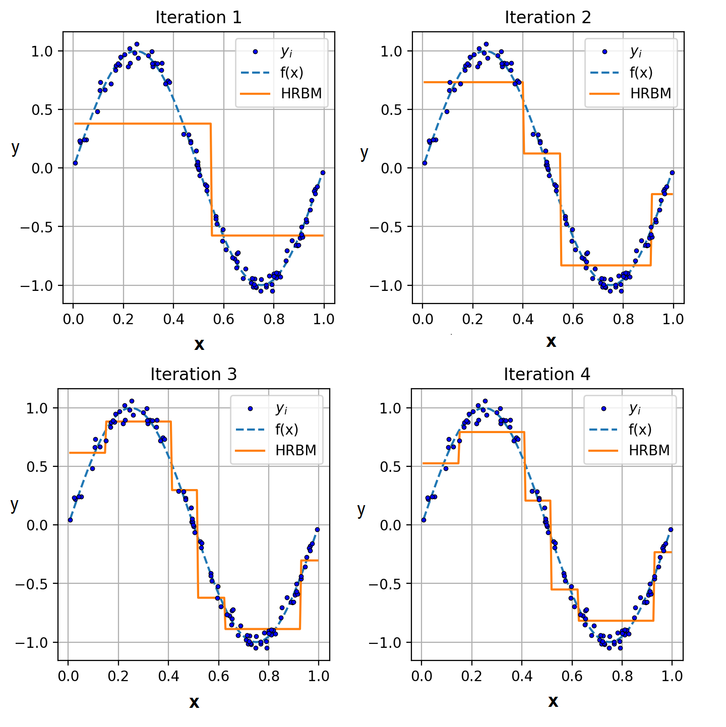
Figure 6: Rectangles generated at four iterations for regression

5 Regularization

In order to improve GBM-HRBM and avoid overfitting, we propose to use regularization. First, we consider the standard $L_{1}$ and $L_{2}$ regularization. Let us add the regularization terms $\Omega(v_{in},v_{out})$ to the loss function $\hat{L}$ defined in (19). A new loss function $\tilde{\mathcal{L}}$ is defined as

$$\tilde{\mathcal{L}}=\hat{L}+\Omega(v_{in},v_{out})=\hat{L}+\lambda_{1}\left|\vec{v}\right|+\frac{\lambda_{2}}{2}\lVert\vec{v}\rVert^{2}$$ (30)

where $\vec{v}=(v_{in},v_{out})^{\mathrm{T}}$; $\lambda_{1}$ and $\lambda_{2}$ are hyperparameters which control the strength of the standard $L_{1}$ and $L_{2}$ regularizations, respectively; $\hat{L}$ is the loss function without regularization defined in (19).

It is simply to get optimal values of $v_{in},v_{out}$ under condition of adding the $L_{1}$ and $L_{2}$ regularization terms. We again use notations introduced in (23) and (24).

Proposition 1

Suppose that the loss function with regularization is of the form (30). If $\lambda_{1}=0$ (the $L_{2}$ regularization), then optimal values of $v_{in}(\lambda_{2})$ and $v_{out}(\lambda_{2})$ as functions of $\lambda_{2}$ are of the form:

$$v_{in}(\lambda_{2})=-\frac{G_{in}}{N\cdot\lambda_{2}+H_{in}},\ v_{out}(\lambda_{2})=-\frac{G_{out}}{N\cdot\lambda_{2}+H_{out}}.$$ (31)

If $\lambda_{1}>0$ and $\lambda_{2}>0$, then the optimal value of $v_{in}(\lambda_{1},\lambda_{2})$ is determined as

$$v_{in}(\lambda_{1},\lambda_{2})=\left\{\begin{array}[c]{cc}-\frac{G_{in}+N\cdot\lambda_{1}}{N\cdot\lambda_{2}+H_{in}},&G_{in}<-N\cdot\lambda_{1},\\ 0,&\left|G_{in}\right|\leq N\cdot\lambda_{1},\\ -\frac{G_{in}-N\cdot\lambda_{1}}{N\cdot\lambda_{2}+H_{in}},&G_{in}>N\cdot\lambda_{1}.\end{array}\right.$$ (32)

$v_{out}(\lambda_{1},\lambda_{2})$ is written similarly if we replace “in” with “out” in (32).

Let us introduce a new type of the regularization function which is called the “step height penalty”. It can be expressed as the distance between $v_{in}$ and $v_{out}$. The idea behind this type of regularization is to minimize the distance between $v_{in}$ and $v_{out}$. In this case, we write the regularization function as

$$\tilde{\mathcal{L}}=\hat{L}+\Omega_{h}(v_{in},v_{out})=\hat{L}+\eta_{1}\left|v_{in}-v_{out}\right|+\frac{\eta_{2}}{2}\lVert v_{in}-v_{out}\rVert^{2}.$$ (33)

Here $\eta_{1}$ and $\eta_{2}$ are hyperparameters which control the strength of the $L_{1}$ and $L_{2}$ regularization terms, respectively.

Proposition 2

Suppose that the loss function with regularization is of the form (33). If $\eta_{1}=0$ (the $L_{2}$-regularization), then optimal values of $v_{in}(\eta_{2})$ and $v_{out}(\eta_{2})$ as functions of $\eta_{2}$ are of the form:

$$v_{in}(\eta_{2})=-\frac{G_{in}+N\eta_{2}G/H_{out}}{H_{in}+N\eta_{2}H/H_{out}},$$ (34)

$$v_{out}(\eta_{2})=-\frac{G_{out}+N\eta_{2}G/H_{in}}{H_{otu}+N\eta_{2}H/H_{in}},$$ (35)

where

$$G=\sum_{i=1}^{N}g_{i},\ H=\sum_{i=1}^{N}h_{i}.$$ (36)

Case $\eta_{1}>0$ does not have a sense because the same regularization can be implemented by using only the case $\eta_{2}>0$ and $\eta_{1}=0$.

It follows from (34) that values of $v_{in}$ and $v_{out}$ by $\eta_{2}>0$ and $\eta_{1}=0$ coincide by large values of $\eta_{2}$, and they are

$$\lim_{\eta_{2}\rightarrow+\infty}v_{in}(\eta_{2})=\lim_{\eta_{2}\rightarrow+\infty}v_{out}(\eta_{2})=\frac{G}{H}.$$ (37)

The above result can be interpreted as follows. If optimal values of $v_{in}$ and $v_{out}$ (without regularization) are far from each other, then the addition of regularization shifts values of $v_{in}$ and $v_{out}$ towards each other.

5.1 Optimal regularization parameters

To ensure the correctness of the approximation of the loss function obtained by means of series expansion (17), as well as to reduce overfitting, it is proposed to restrict the absolute values of function $f_{k}(\mathbf{x})$. The first way implementing the restriction is to multiply function $f_{k}(\mathbf{x})$ by the learning rate $\gamma$. The second way is based on regularization which has been studied in Propositions 1 and 2.

First, we consider the standard $L_{1}$ and $L_{2}$ regularization (30). Values of the regularization parameters $\lambda_{1}$ and $\lambda_{2}$ can be estimated by bounding the HRBM absolute values by some constant $\beta$ which can be regarded as an analogue of the learning rate that limits each rectangle:

$$\left|f_{k}(\mathbf{x})\right|\leq\beta.$$ (38)

The following proposition establishes the relationship between parameters $\lambda_{1}$, $\lambda_{2}$ and $\beta$ when the $L_{1}$ or $L_{2}$ regularization is used.

Proposition 3

Suppose that the loss function with regularization is of the form (30), and the condition (38) is fulfilled. Then the optimal value $\underline{\lambda}_{2}$ of $\lambda_{2}$ as a function of $\beta$ is defined as follows:

$$\underline{\lambda}_{2}=\max\left({\underline{\lambda}_{2}^{in},\underline{\lambda}_{2}^{out},0}\right),$$ (39)

where

$$\underline{\lambda}_{2}^{in}=\frac{1}{N}\left[\frac{1}{\beta}\left|G_{in}\right|-H_{in}\right],$$ (40)

$$\underline{\lambda}_{2}^{out}=\frac{1}{N}\left[\frac{1}{\beta}\left|G_{out}\right|-H_{out}\right].$$ (41)

The optimal value $\overline{\lambda}_{1}$ of $\lambda_{1}$ as a function of $\beta$ is defined as follows:

$$\overline{\lambda}_{1}=\min(\overline{\lambda}_{1}^{in},\overline{\lambda}_{1}^{out}).$$ (42)

where

$$\overline{\lambda}_{1}^{in}=\frac{1}{N}[\beta H_{in}-|G_{in}|],$$ (43)

$$\overline{\lambda}_{1}^{out}=\frac{1}{N}[\beta H_{out}-|G_{out}|].$$ (44)

By using the above approach to choosing $\lambda_{1}$ or $\lambda_{2}$, we can state that one of the values of $v_{in}$ or $v_{out}$ is equal to $\beta$ (except for the case when the first derivative is zero for the entire dataset, i.e., $\forall i:~{}g_{i}=0$). Then the second value does not exceed $\beta$.

Let us consider again the condition (38) under condition that the regularization parameters $\eta_{1}$ and $\eta_{2}$ are defined by the step height penalty (33). First, we study the case when $\eta_{1}=0$.

Proposition 4

Suppose that the loss function with regularization is of the form (33), and condition (38) is fulfilled. Denote

$$C_{1}=\frac{H_{out}}{N}\frac{G_{in}+\beta H_{in}}{G+\beta H},\ C_{2}=-\frac{H_{out}}{N}\frac{G_{in}+\beta H_{in}}{G-\beta H},$$ (45)

$${B_{1}=-\frac{H_{in}}{N}\frac{G_{out}+\beta H_{out}}{G+\beta H},\ }B_{2}={\frac{H_{out}}{N}\frac{-G_{in}+\beta H_{in}}{G-\beta H},}$$ (46)

$${B_{3}=\frac{H_{in}}{N}\frac{-G_{out}+\beta H_{out}}{G-\beta H}.}$$ (47)

Then the optimal value $\underline{\eta}_{2}$ of $\eta_{2}$ as a function of $\beta$ for $v_{in}$ is defined depending on three cases as follows:

If $G>\beta H$, then $\underline{\eta}_{2}=C_{1}$ for $v_{in}$ and $\underline{\eta}_{2}=\max\left({0,-C}_{1}{,-B_{1}}\right)$ for $v_{out}$.

If $|G|<\beta H$, then $\underline{\eta}_{2}=\max\left(C_{2}{,}C_{1}\right)$ for $v_{in}$ and $\underline{\eta}_{2}=\max({0,B_{1},B_{2},{B}_{3},C_{2})}$ for $v_{out}$.

If $G<-\beta H$, then $\underline{\eta}_{2}=C_{2}$ for $v_{in}$ and $\underline{\eta}_{2}=\max\left({0,}B_{2}{,B_{3}}\right)$ for $v_{out}$.

We have obtained simple expressions for choosing optimal values of the regularization parameters. It should be noted that they depend on the parameter $\beta$ which is unknown. The main advantage of using the parameter $\beta$ instead of parameters $\lambda_{1}$ and $\lambda_{2}$ or $\eta_{1}$ and $\eta_{2}$ is that $\beta$ is not changed at each iteration of GBM-HRBM whereas parameters $\lambda_{1}$, $\lambda_{2}$, $\eta_{1}$, $\eta_{2}$ are defined for each iteration and depend on the corresponding residuals obtained after the previous iteration. If the number of iterations in GBM-HRBM is $T$, then the lower value of $\beta$ is defined from the following reasons. The final prediction of GBM-HRBM is $F_{T}(\mathbf{x})$. Its absolute value is bounded by absolute values of functions $f_{k}(\mathbf{x})$ and by parameter $\beta$ as

$$\left|F_{T}(\mathbf{x})\right|\leq\sum_{k=1}^{T}\left|f_{k}(\mathbf{x})\right|\leq T\beta.$$ (48)

The above implies that $\beta$ is bounded as

$$\beta\geq\max_{\mathbf{x}\in D}\frac{\left|F_{T}(\mathbf{x})\right|}{T}$$ (49)

The upper bound can be arbitrary, for example, $\beta\leq\max\left|F_{T}(\mathbf{x})\right|$.

6 Algorithms for training and predicting GBM-HRBM

We provide algorithms for training and predicting GBM-HRBM. First, we consider algorithms for generating optimal rectangles of two types: closed rectangles and corners. Second, we show a whole algorithm for implementing GBM-HRBM and its components.

6.1 Algorithms for generating rectangles

The optimal rectangle generation is an essential component of GBM-HRBM. Therefore, the main idea of Algorithm 1 is to generate many ($K$) rectangles at each iteration of GBM and to select the best one which minimizes a cost function $C_{\theta}$. In spite of a general form of optimization problems (lines 2 and 3 of the algorithm), values $v_{in}$ and $v_{out}$ (lines 2 and 3 of the algorithm) can be computed by using (21) without solving the optimization problems.

Algorithm 1 Optimal Rectangle Generation

1:Data set $D$, number of generated rectangles $K$

2:Parameters $\theta=(\mathbf{r},v_{in},v_{out})$ of a filled rectangle $\mathbf{r}$

3:function Fill($r,D$) $\triangleright$ A function of choosing optimal parameters of a rectangle

4:     $v_{in}\leftarrow\arg\min_{v}\sum_{(\mathbf{x},y)\in D}l(y,v)\cdot\mathbb{I}[\mathbf{x}\in\mathbf{r}]$

5:     $v_{out}\leftarrow\arg\min_{v}\sum_{(\mathbf{x},y)\in D}l(y,v)\cdot\mathbb{I}[\mathbf{x}\notin\mathbf{r}]$

6:     return $v_{in},v_{out}$

7:end function

8:for $i\in{1,\dots,K}$ do

9:     $\mathbf{r}\leftarrow$Generate(D)$\triangleright$ Generating a random rectangle

10:     $v_{in},v_{out}\leftarrow$Fill(r, D) $\triangleright$ Choosing optimal values $v_{in},v_{out}$ for the rectangle $\bf{r}$

11:     $\theta\leftarrow(\mathbf{r},v_{in},v_{out})$

12:     $C_{\theta}\leftarrow\sum_{(\mathbf{x},y)\in D}\left(l(y,v_{in})\cdot\mathbb{I}[\mathbf{x}\in\mathbf{r}]+l(y,v_{out})\cdot\mathbb{I}[\mathbf{x}\notin\mathbf{r}]\right)$

13:end for

14:$\theta\leftarrow\arg\min_{\theta}C_{\theta}$

15:return $\theta$

Depending on a type of generated rectangles, we consider two algorithms of the function Generate(). The first one is based on random selection of a center $\mathbf{c}$ and sizes $w_{1},...,w_{d}$ of each rectangle. Centers of rectangles are generated from the uniform distribution with parameters defined by the largest $b^{(j)}$ and smallest $a^{(j)}$ coordinates of all points from the dataset $D$. In order to cover at least one data point by each rectangle, we find the nearest point $\alpha$ and farthest point $\beta$ from the $j$-th coordinate $c^{(j)}$ of the generated center of the rectangle. The width $\mathbf{w}$ of each rectangle depends on the corresponding distance between the nearest $\alpha$ (the farthest $\beta$) point and the center. It is shown as Algorithm 2. The second algorithm of the function Generate() is based on random selection of a corner (the rectangle center $\mathbf{c}$) and unbounded elements of vectors $\mathbf{a}$ and $\mathbf{b}$. It is shown as Algorithm 3.

Algorithm 2 Random Rectangle Generation

1:Data set $D$

2:Generated rectangle $\mathbf{r}$ in the form of closed rectangle

3:for $j\in{1,\dots,d}$ do

4:     $a^{(j)}\leftarrow\min\left\{{x_{i}^{(j)}|(\mathbf{x}_{i},y_{i})\in D}\right\}$ $\triangleright$ Smallest values of features

5:     $b^{(j)}\leftarrow\max\left\{{x_{i}^{(j)}|(\mathbf{x}_{i},y_{i})\in D}\right\}$ $\triangleright$ Largest values of features

6:     $c^{(j)}\sim\mathcal{U}[a^{(j)},b^{(j)}]$ $\triangleright$ The center of a rectangle is generated from the uniform distribution

7:     $\alpha\leftarrow\min_{i=1,...,n}\left|x_{i}^{(j)}-c^{(j)}\right|$ $\triangleright$ The smallest distance between the center and data points

8:     $\beta\leftarrow\max_{i=1,...,n}\left|x_{i}^{(j)}-c^{(j)}\right|$$\triangleright$ The largest distance between the center and data points

9:     $w^{(j)}\sim\mathcal{U}[\alpha,\beta]$ $\triangleright$ The rectangle width

10:     $r^{(j)}\leftarrow[c^{(j)}-w^{(j)}/2,c^{(j)}+w^{(j)}/2]$

11:end for

12:return $\mathbf{r}$

Algorithm 3 Random Corner Generation

1:Data set $D$

2:Generated rectangle in the form of corner $\mathbf{r}$

3:for $j\in{1,\dots,d}$ do

4:     $a^{(j)}\leftarrow\min\left\{{x_{i}^{(j)}|(\mathbf{x}_{i},y_{i})\in D}\right\}$ $\triangleright$ Smallest values of features

5:     $b^{(j)}\leftarrow\max\left\{{x_{i}^{(j)}|(\mathbf{x}_{i},y_{i})\in D}\right\}$ $\triangleright$ Largest values of features

6:     $c^{(j)}\sim\mathcal{U}[a_{j},b_{j}]$ $\triangleright$ A center of the cornor generated from the uniform distribution

7:     $\zeta\sim\text{Bernoulli}(0.5)$

8:     if $\zeta=0$ then

9:         $a^{(j)}\leftarrow-\infty$ and $b^{(j)}\leftarrow c^{(j)}$

10:     else

11:         $a^{(j)}\leftarrow c^{(j)}$ and $b^{(j)}\leftarrow\infty$

12:     end if

13:end for

14:return $\mathbf{r}$

6.2 The whole algorithm of GBM-HRBM

Algorithm 4 illustrates GBM with HRBMs. In the algorithm, we deliberately add rectangles with a zero outside value $v_{out}$ to the resulting set $R$ taking out the sum of all outside values into the common bias term $q$. This trick allows us to predict faster. The function Split() divides training set $D$ into the training subset $D_{train}$ and the validation subset $D_{val}$. The function MakeRectangle() generates rectangles, but it is slightly different from the similar function in Algorithm 1. The difference is that filling of rectangles (Fill()) is performed by using the already calculated values $g$ and $h$ in (19). The function IsValid() controls whether a new rectangle provides a smaller value of the loss function on the validation subset.

Algorithm 4 The whole training algorithm of GBM-HRBM

1:Training data $D$; twice differentiable loss function $l$; number of iterations for generating rectangles $M$; learning rate $\gamma$; number of validation attempts $V$

2:The output rectangle set $R$; bias $q$

3:function IsValid($D_{val},s,\theta$)

4:     $C_{val}\leftarrow\sum_{(\mathbf{x}_{i},y_{i})\in D_{val}}l(y_{i},s_{i})$

5:     $C_{new}\leftarrow\sum_{(\mathbf{x}_{i},y_{i})\in D_{val}}l(y_{i},s_{i}+\textsc{Predict}(\theta,x_{i}))$

6:     if $C_{new}\leq C_{val}$ then

7:         return True

8:     else

9:         return False

10:     end if

11:end function

12:$q\leftarrow\arg\min_{q}\sum_{(\mathbf{x}_{i},y_{i})\in D}l(y_{i},q)$ $\triangleright$ Initialize the bias term

13:$\mathbf{s}=(q,\dots,q)^{T}$ $\triangleright$ Initialize the cumulative prediction sum

14:$(D_{train},D_{val})\leftarrow\textsc{Split}(D)$ $\triangleright$ Split dataset into the training and validation subsets

15:$R\leftarrow\emptyset$ $\triangleright$ Initialize the resulting rectangle set

16:$\triangleright$ Initial prediction for the $i$-th point is $b$

17:for $k\in\{1,\dots,K\}$ do

18:     for $(x_{i},y_{i})\in D_{train}$ do

19:         $\left.g_{i}\leftarrow\frac{\partial l(y_{i},z)}{\partial z}\right|_{z=s_{i}}$

20:         $\left.h_{i}\leftarrow\frac{\partial^{2}l(y_{i},z)}{\partial z^{2}}\right|_{z=s_{i}}$

21:     end for

22:     for $j\in\{1,\dots,V\}$ do

23:         $\theta\leftarrow\textsc{MakeRectangle}(D_{train},g,h,l,M)$

24:         if IsValid($D_{val},s,\theta$) then $\triangleright$ If the rectangle passes validation, then add the rectangle

25:              $(\mathbf{r},v_{in},v_{out})\leftarrow\theta$

26:              $q\leftarrow q+\gamma\cdot v_{out}$

27:              for $(x_{i},y_{i})\in D$ do

28:                  $\mathbf{s}_{i}\leftarrow\mathbf{s}_{i}+\gamma\cdot\mathbb{I}[\mathbf{x}_{i}\in\mathbf{r}]\cdot(v_{in}-v_{out})+\gamma\cdot v_{out}$

29:              end for

30:              $R\leftarrow R\cup\left\{\left(\mathbf{r},\gamma\cdot(v_{in}-v_{out}),0\right)\right\}$ $\triangleright$ Addition of the rectangle to the output rectangle set

31:              $(D_{train},D_{val})\leftarrow\textsc{Split}(D)$ $\triangleright$ Split the dataset

32:              break

33:         end if

34:     end for

35:end for

36:return $R,b$

6.3 Prediction algorithm

The prediction algorithm, which implements computing the prediction $y$ for a new example $\mathbf{x}$, is represented as Algorithm 5.

Algorithm 5 The prediction algorithm

1:Data point for prediction $\mathbf{x}$; rectangle set $R$; common bias $q$

2:Prediction $y$ corresponding to $\mathbf{x}$

3:$y=q$ $\triangleright$ Initialize a cumulative prediction sum

4:for $\theta\in R$ do

5:     $(\mathbf{r},v_{in},0)\leftarrow\theta$ $\triangleright$ When the ensemble is built, all values $v_{out}=0$

6:     $y\leftarrow y+\mathbb{I}[\mathbf{x}\in\mathbf{r}]\cdot v_{in}$

7:end for

8:return $y$

7 Interpretability of GBM-HRBM

Interpretation means that important features of an analyzed explained example have to be selected, which significantly impact on the corresponding prediction provided by a black-box model. By considering interpretation of a single example, we say about the so-called local interpretation methods [62]. They aim to interpret predictions of a black-box model locally around the considered example. Another (global) interpretation methods try to interpret predictions taking into account the whole dataset or its certain part.

One of the most popular post-hoc approaches to interpretation is the well-known method SHAP [27, 28]. SHAP is widely used in practice and can be viewed as the most promising and theoretically justified explanation method which fulfils several nice properties [27]. It uses Shapley values [29] as a concept in coalitional games. According to the concept, the total gain of a game is distributed among players such that desirable properties, including efficiency, symmetry, and linearity, dummy are fulfilled. In the framework of the machine learning, the gain can be viewed as the machine learning model prediction or the model output, and a player is a feature of input data. Hence, contributions of features to the model prediction can be estimated by Shapley values, and the $i$-th feature importance is defined by the Shapley value denoted as $\phi_{i}$.

Suppose that a prediction $f(\mathbf{x})$ has to be explained for a point $\mathbf{x}\in\mathbb{R}^{d}$. Denote the index subset of $M=\{1,...,d\}$ as $S\subseteq M$ and a subset of $k$ features with indices from $S=\{i_{1},...,i_{k}\}$ as $\mathbf{x}^{(S)}=(x^{(i_{1})},...,x^{(i_{k})})$. Let us also denote $f(\mathbf{x}^{(S)})$ as $\Psi(S)$ for a given $\mathbf{x}$ and $f$.

Shapley values have the following well-known properties:

Efficiency. The total gain is distributed as

$$\sum_{i=1}^{d}\phi_{k}=\Psi(M)-\Psi(\emptyset).$$ (50)

Symmetry. If two players with numbers $i$ and $j$ make equal contributions, i.e., there holds

$$\Psi\left(S\cup\{i\}\right)=\Psi\left(S\cup\{j\}\right)$$ (51)

for all subsets $S$ which contain neither $i$ nor $j$, then $\phi_{i}=\phi_{j}$.

Linearity. A linear combination of multiple games $f_{1},...,f_{m}$, represented as $f(S)=\sum_{k=1}^{m}c_{k}f_{k}(S)$, has gains derived from $f$: $\phi_{i}(f)=\sum_{k=1}^{m}c_{k}\phi_{i}(f_{k})$ for every $i$.

Dummy. If a player makes zero contribution, i.e., $\Psi\left(S\cup\{j\}\right)=\Psi\left(S\right)$ for a player $j$ and all $S\subseteq M\backslash\{j\}$, then $\phi_{j}=0$.

If all the above properties are satisfied, then we can write the following expression for computing Shapley values:

$$\phi_{i}=\sum_{S\subseteq M\backslash\{i\}}\frac{\#S!\left(d-\#S-1\right)!}{d!}\left[\Psi\left(S\cup\{i\}\right)-\Psi\left(S\right)\right],$$ (52)

where $\#S$ is the number of elements in $S$.

Let us define the method for calculating the feature subset function $\Psi(S)$ for HRBM as follows:

$$\Psi(S)=\mathbb{I}[\mathbf{x}^{(S)}\in\mathbf{r}^{(S)}]\cdot(v_{in}-v_{out})+v_{out},$$ (53)

where $\mathbf{r}^{(S)}$ is a rectangle that includes only features with indices from subset $S$.

For the empty set of features, it is natural to set the value of the indicator function equal to 1. Then there holds:

$$\Psi(\emptyset)=(v_{in}-v_{out})+v_{out}=v_{in}.$$ (54)

Proposition 5

The contribution of the $i$-th feature of HRBM is determined as follows:

$$\phi_{i}=\begin{cases}0,&x^{(i)}\in r^{(j)},\\ \dfrac{v_{out}-v_{in}}{\sum_{j=1}^{d}\mathbb{I}[x^{(i)}\notin r^{(j)}]},&x^{(i)}\notin r^{(j)}.\end{cases}$$ (55)

The main advantage of this approach is its isolation from the training data set: the calculated contributions depend solely on the structure of the model (rectangles and their inside values), but do not depend on the data, allowing us to explore with their help separately the behavior of the model. That is why we call the method as the model-based SHAP. On the other hand, this approach does not take into account how the model predictions are supported by the training data, which makes it difficult to extract useful information about the task. Therefore, we consider also an original definition [27] of the function of a subset of features through expectations:

$$\tilde{\Psi}(S)=\mathbb{E}[f(X)\mid X_{S}=\mathbf{x}^{(S)}],$$ (56)

$$\tilde{\Psi}(\emptyset)=\mathbb{E}[f(X)].$$ (57)

This method is called the data-based SHAP.

Proposition 6

By using the original definition of Shapley values through expectations [27], the contribution $\phi_{i}$ of the $i$-th feature of HRBM is determined as follows:

For each $i$-th feature such that $x^{(i)}\notin r^{(i)}$, there holds $\phi_{i}=\tilde{\phi}$, otherwise the contribution $\phi_{i}$ is computed as

$$\phi_{i}=\sum_{S\subset\{1,\dots,d\}\setminus\{i\}}\frac{\left|S\right|!(d-\left|S\right|-1)!}{d!}(\tilde{\Psi}(S\cup\{i\})-\tilde{\Psi}(S)),$$ (58)

where

$$\tilde{\Psi}(S\cup\{i\})-\tilde{\Psi}(S) =\frac{v_{in}-v_{out}}{N}\cdot\mathbb{I}[\mathbf{x}^{(S)}\in\mathbf{r}^{(S)}]$$

$$\times\sum_{t=1}^{N}\mathbb{I}[\mathbf{x}_{t}^{(\overline{S}\setminus\{i\})} \in\mathbf{r}^{(\overline{S}\setminus\{i\})}]\cdot\mathbb{I}[x_{t}^{(i)}\notin r^{(i)}].$$ (59)

Here $\overline{S}=M\setminus S$ is the set of features which are not included in $S$. The sum in (58) is calculated only for subsets $S$ which fulfil condition $\mathbf{x}^{(S)}\in\mathbf{r}^{(S)}$.

Value $\tilde{\phi}$ is calculated from the efficiency property as

$$\tilde{\phi}=\frac{\tilde{\Psi}(\{1,\dots,d\})-\tilde{\Psi}(\emptyset)-\sum_{i=1}^{d}\phi_{i}\cdot\mathbb{I}[x^{(i)}\in r^{(i)}]}{\sum_{j=1}^{d}\mathbb{I}[x^{(j)}\notin r^{(j)}]}.$$ (60)

Thus, we need first to find values for all features for which the explained example is inside the rectangle using (58), and then using (60) to calculate Shapley values for the remaining features. In order to obtain Shapley values for an arbitrary HRBM ensemble, for example, boosting, we use the third property (linearity) of Shapley values. According to this property, the contribution of each feature of the weighted ensemble is represented as the sum of the contributions of each model with the appropriate weights.

Remark 1

It is important to point out that the considered GBM-HRBM is not a black-box model because, in addition to the input data and predictions of the model, we use information about generated rectangles at iterations of the boosting. On the other hand, GBM-HRBM can be used as an interpretable meta-model approximating some black-box model, for instance, a deep neural network. Moreover, GBM-HRBM can play a double role. First, it can be regarded as an interpretable approximating model like the linear model. In this case, GBM-HRBM is trained on the feature vectors and the corresponding predicted values provided by the black-box model. As a result, GBM-HRBM extends the set of interpretable models. Second, GBM-HRBM can be viewed as a student model for the teacher black-box model in the knowledge distillation framework. In addition, GBM-HRBM can be the interpretable meta-model approximating the black-box model and a student model in distillation similarly to the DeepVID model [77].

8 Numerical experiments

In order to study the proposed GBM-HRBM for solving regression problems, we apply datasets which are taken from open sources, in particular: Diabetes can be found in the corresponding R Packages; Friedman 1, 2 3 are described at site: https://www.stat.berkeley.edu/~breiman/bagging.pdf; Scikit-Learn Sparse Uncorrelated (Sparse) datasets are available in package “Scikit-Learn”. The proposed algorithm is evaluated and investigated also by the following publicly available datasets from the UCI Machine Learning Repository [78] (short notations are given in brackets): Auto MPG, Boston Housing (Boston), Concrete, Forest Fires, Yacht Hydrodynamics (Yacht), Airfoil. We also use datasets Chscase_Census2 (CCC2), ERA, FruitFly, Fish Catch, LiverDisorders, MachineCPU from OpenML https://www.openml.org. A brief introduction about these data sets are given in Table 1 where $d$ and $N$ are numbers of features and examples, respectively. A more detailed information can be found from the aforementioned data resources.

Table 1: A brief introduction about datasets for regression

Dataset	$d$	$N$	Dataset	$d$	$N$
Airfoil	$5$	$1503$	Friedman1	$10$	$100$
AutoMpg	$8$	$398$	Friedman2	$4$	$100$
Boston	$13$	$506$	Friedman3	$4$	$100$
CCC2	$8$	$400$	FruitFly	$5$	$125$
Concrete	$8$	$1030$	LiverDisorders	$6$	$345$
Diabetes	$10$	$442$	MachineCPU	$7$	$209$
ERA	$4$	$1000$	Sparse	$10$	$100$
FishCatch	$7$	$159$	Yacht	$6$	$308$
ForestFire	$13$	$517$

We use the coefficient of determination denoted $R^{2}$ for the regression evaluation. The greater the value of the coefficient of determination, the better results we get. The best results in all tables are shown in bold. $F_{1}$ score is used in the classification experiments as an accuracy measure which takes into account the possible class imbalance.

The proposed GBM-HRBM model is compared with ensemble-based models including RFs, ERTs, and GBM with decision trees as base models. Numbers of trees $100$, $200$, $300$, $400$, $500$ in RFs and ERTs are tested, choosing those leading to the best results.

In order to optimize the model parameters in numerical experiments, we perform a 5-fold cross-validation on the training set which consists of different numbers of randomly selected examples. The cross-validation is performed with $50$ repetitions. This procedure is realized by considering all possible values of the regularization parameter $\beta$ and other tuning parameters in a predefined grid. Their values are also tested, choosing those leading to the best results.

The code implementing GBM-HRBM can be found at: https://github.com/andruekonst/HRBM.

8.1 Regression

In order to compare GBM-HRBM with other ensemble-based models, measures $R^{2}$ for the RF, ERT, GBM with decision trees as base models, and for GBM-HRBM are computed for several real datasets and shown in Table 2.  Measures $R^{2}$ for GBM-HRBM are obtained as the best values among two types of HRBMs: rectangles and corners. It can be seen from Table 2 that GBM-HRBM outperforms the aforementioned ensemble-based models for 13 from 17 datasets. Moreover, the difference between values of $R^{2}$ is large for datasets Sparse ($0.124$), Diabetes ($0.046$), Fridman1 ($0.041$). At the same time, there are datasets (Airfoil, Concrete, Friedman2, Yacht) for which one of the models (RF, ERT, GBM) provide better results in comparison with GBM-HRBM.

Let us compare values of $R^{2}$ obtained for GBM-HRBM with the best results provided by one of the models: RF, ERT, GBM. For comparison, we can apply the $t$-test. According to [79], the $t$-statistics is distributed in accordance with the Student distribution with $17-1$ degrees of freedom ($17$ datasets). The obtained p-value is $p=0.045$. We can conclude that the outperformance of GBM-HRBM is statistically significant because $p<0.05$.

Table 2: $R^{2}$ measures for comparison of the RF, ERT, GBM, GBM-HRBM in the regression tasks

Dataset	RF	ERT	GBM	GBM-HRBM
Airfoil	$0.909$	$0.910$	$\mathbf{0.952}$	$0.922$
AutoMpg	$0.870$	$0.871$	$0.863$	$\mathbf{0.882}$
Boston	$0.859$	$0.863$	$0.861$	$\mathbf{0.876}$
CCC2	$-0.048$	$-0.030$	$-0.022$	$\mathbf{-0.018}$
Concrete	$0.898$	$0.901$	$\mathbf{0.933}$	$0.927$
Diabetes	$0.426$	$0.431$	$0.422$	$\mathbf{0.477}$
ERA	$0.361$	$0.360$	$0.361$	$\mathbf{0.364}$
FishCatch	$0.951$	$0.957$	$0.948$	$\mathbf{0.974}$
ForestFire	$-0.014$	$-0.013$	$-0.012$	$\mathbf{-0.009}$
Friedman1	$0.778$	$0.803$	$0.880$	$\mathbf{0.921}$
Friedman2	$0.983$	$\mathbf{0.994}$	$0.986$	$0.991$
Friedman3	$0.874$	$0.921$	$0.908$	$\mathbf{0.923}$
FruitFly	$-0.102$	$-0.099$	$-0.087$	$\mathbf{-0.051}$
LiverDisorders	$0.160$	$0.162$	$0.126$	$\mathbf{0.201}$
MachineCPU	$0.864$	$0.856$	$0.827$	$\mathbf{0.872}$
Sparse	$0.627$	$0.682$	$0.681$	$\mathbf{0.811}$
Yacht	$0.995$	$0.995$	$\mathbf{0.998}$	$0.996$

Another interesting question is how different types of the regularization impact on the accuracy of GBM-HRBM. We compare three types of regularization, including the $L_{2}$-norm of step height penalty (see (33)), the $L_{1}$- and $L_{2}$-norms of the standard regularization (see (30)). The corresponding values of $R^{2}$ are shown in Table 3. One can see from Table 3 that it is difficult to select the best type of regularization. Each type demonstrates outperforming results for several datasets. Therefore, it makes sense to analyze all types of regularization for new datasets.

Table 3: $R^{2}$ measures for comparison of different types of regularization for GBM-HRBM

Dataset	Step height penalty $L_{2}$	Standard $L_{1}$	Standard $L_{2}$
Airfoil	$0.879$	$0.873$	$\mathbf{0.922}$
AutoMpg	$0.881$	$\mathbf{0.882}$	$0.881$
Boston	$\mathbf{0.876}$	$0.866$	$0.873$
CCC2	$\mathbf{-0.018}$	$\mathbf{-0.018}$	$\mathbf{-0.018}$
Concrete	$0.925$	$0.911$	$\mathbf{0.927}$
Diabetes	$\mathbf{0.477}$	$0.473$	$\mathbf{0.477}$
ERA	$\mathbf{0.364}$	$\mathbf{0.364}$	$0.363$
FishCatch	$\mathbf{0.974}$	$\mathbf{0.974}$	$\mathbf{0.974}$
ForestFire	$-0.010$	$-0.010$	$\mathbf{-0.009}$
Friedman1	$\mathbf{0.921}$	$0.906$	$0.920$
Friedman2	$\mathbf{0.991}$	$0.982$	$0.990$
Friedman3	$0.917$	$0.885$	$\mathbf{0.923}$
FruitFly	$\mathbf{-0.051}$	$\mathbf{-0.051}$	$-0.052$
LiverDisorders	$0.188$	$0.188$	$\mathbf{0.201}$
MachineCPU	$0.870$	$0.869$	$\mathbf{0.872}$
Sparse	$0.808$	$0.773$	$\mathbf{0.811}$
Yacht	$0.995$	$0.989$	$\mathbf{0.996}$

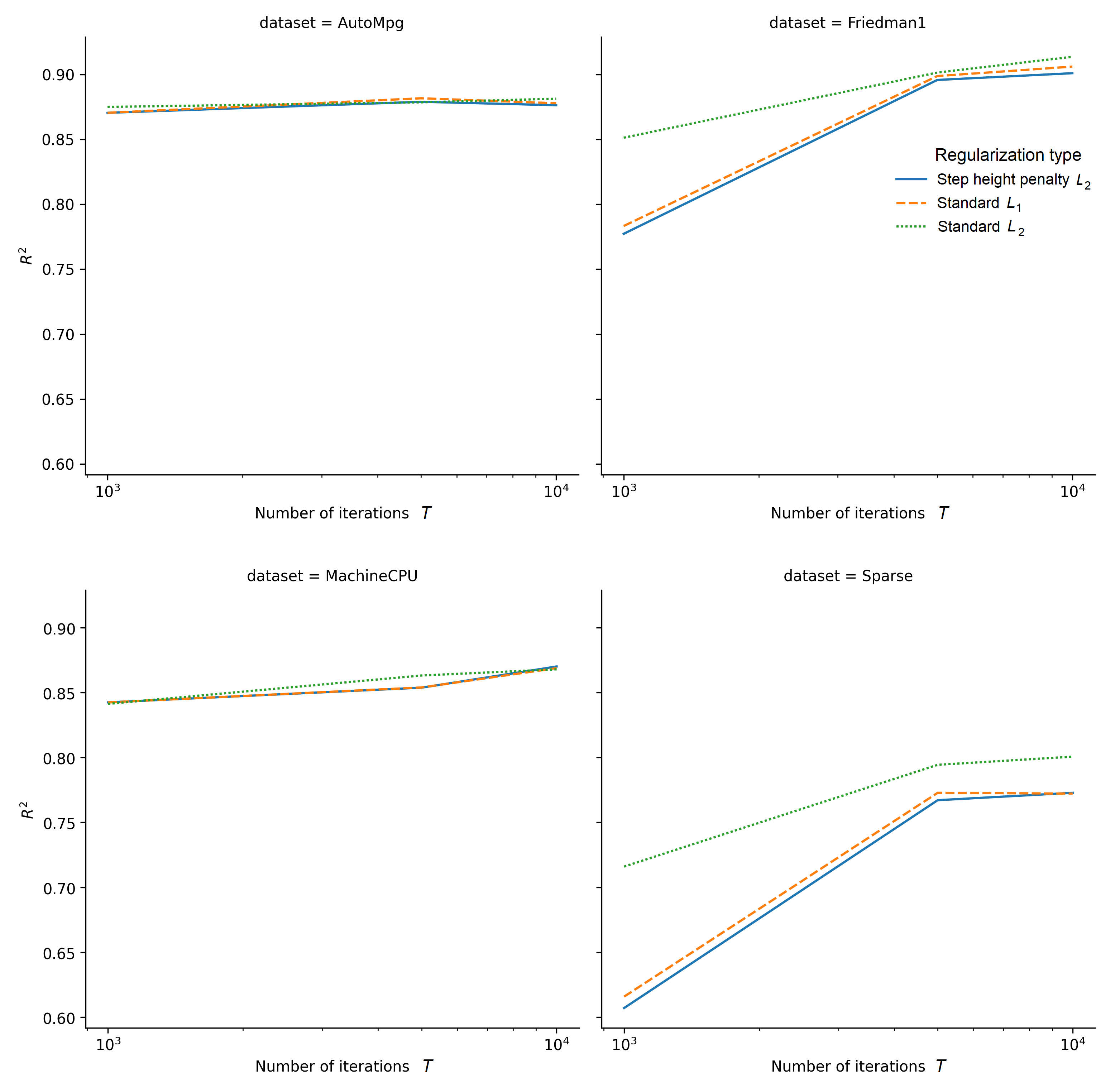
Figure 7: $R^{2}$ as a function of the number of the GBM-HRBM iterations for four datasets by different regularization types

Fig. 7 shows how the model accuracy depends on the number of iterations $T$ for four datasets (AutoMpg, Friedman1, MachineCPU, Sparse) under condition of using three regularization types (step height penalty using Proposition 2 and standard $L_{1}$, $L_{2}$ regularizations using Proposition 1). The step height penalty and standard $L_{1}$, $L_{2}$ regularizations are depicted by solid, dashed and dotted lines. One can see from Fig. 7 that $R^{2}$ increases with the number of iterations. However, after some number of iterations, the accuracy almost does not increase. It can also be seen from Fig. 7 that the regularization type does not significantly impact on the accuracy except for the case of Friedman1 and Sparse datasets where the standard $L_{2}$ regularization provides better results.

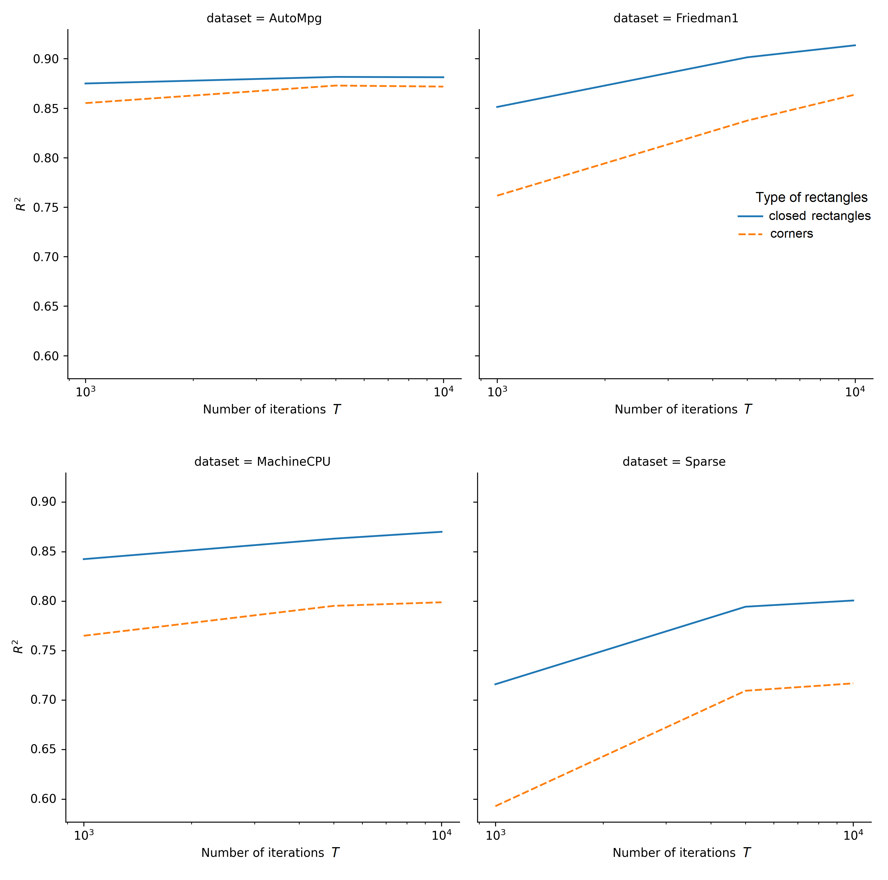
Figure 8: $R^{2}$ as a function of the number of the GBM-HRBM iterations for four datasets by different types of rectangles

The same dependencies of $R^{2}$ on numbers of iterations are shown in Fig. 8, but, in contrast to the previous experiment, we study how the type of rectangles impacts on the accuracy. Functions under conditions of using corners and closed rectangles are depicted by the solid and dashed lines respectively. It can be seen from Fig. 8 that the tendency of functions does not differ from the same functions in Fig. 7. However, the model with corners outperforms the model with closed rectangles.

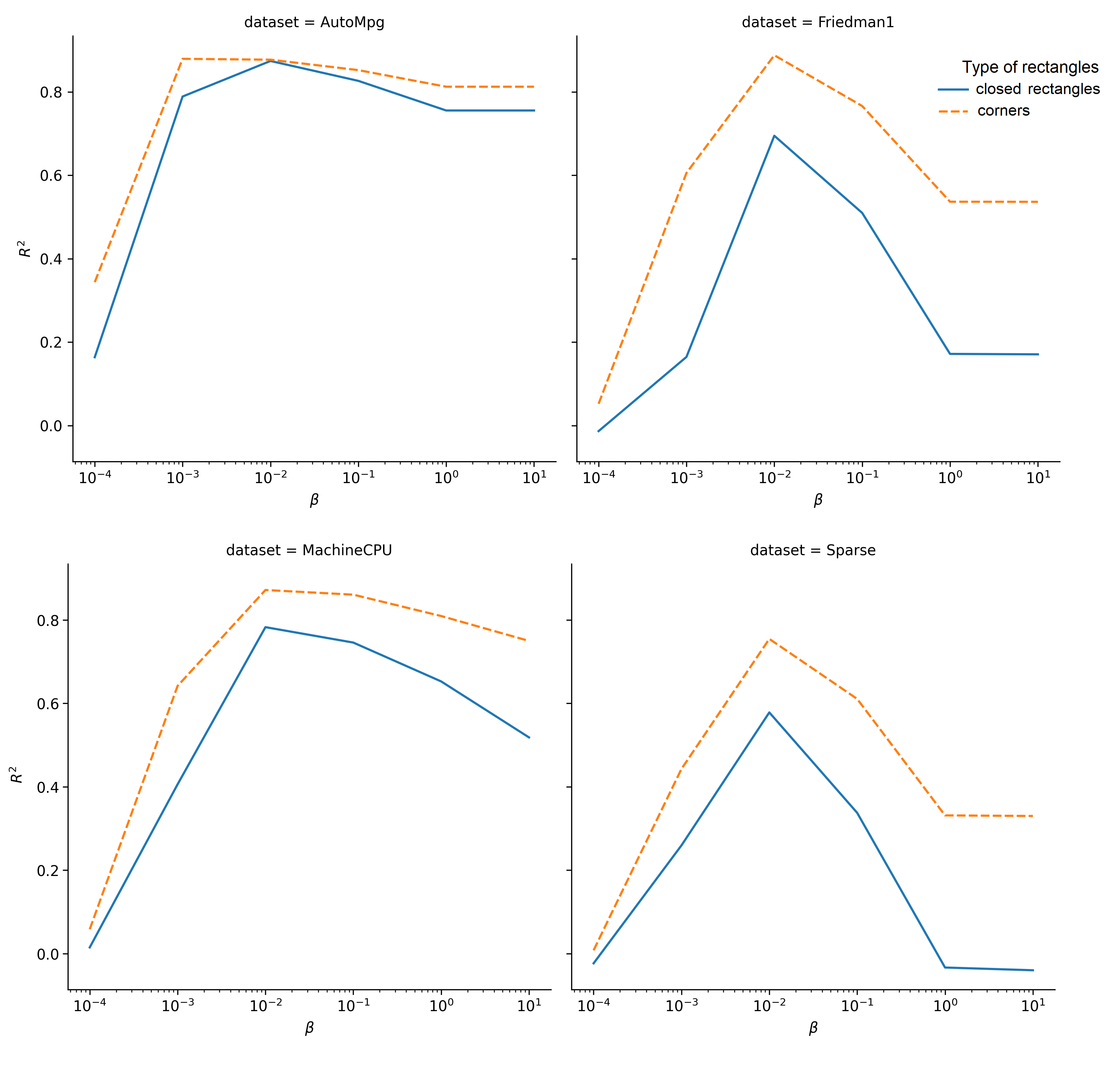
Figure 9: $R^{2}$ as a function of the regularization parameter $\beta$ for four datasets (AutoMpg, Friedman1, MachineCPU, Sparse) by using corners and closed rectangles

The next question is how the $R^{2}$ measure depends on the regularization parameter $\beta$. We consider the standard $L_{2}$ regularization (30). The corresponding dependencies are depicted in Fig. 9 where GBM-HRBM with the $L_{2}$ regularization is trained on the same four regression datasets (AutoMpg, Friedman1, MachineCPU, Sparse) with a fixed number of iterations of GBM-HRBM. Moreover, two HRBMs are studied for every dataset: corners and closed rectangles depicted by dashed and solid lines, respectively. It can be seen from Fig. 9 that there exists an optimal value of $\beta$ for all datasets. This peculiarity is very important because we do not need to tune the parameter $\lambda_{2}$ at each iteration of GBM-HRBM. We tune only $\beta$ and compute different $\lambda_{2}$ at each iteration by using Proposition 3. Another interesting observation from Fig. 9 is that GBM-HRBM with corners shows better results in comparison with GBM-HRBM with closed rectangles almost for all $\beta$. In order to confirm this observation, we consider corners and closed rectangles for other datasets. The corresponding values of $R^{2}$ are shown in Table 4. It is seen from the results that corners provide outperforming results for most datasets. If we again apply the $t$-test to these results, then we obtain p-value equal to $p=0.004$. It is obvious that corners give the statistically significant outperformance.

Table 4: $R^{2}$ measures for comparison of different types of rectangles: corners and closed rectangles

Dataset	Corners	Rectangles
Airfoil	$\mathbf{0.922}$	$0.891$
AutoMpg	$\mathbf{0.882}$	$0.877$
Boston	$\mathbf{0.876}$	$0.857$
CCC2	$\mathbf{-0.018}$	$\mathbf{-0.018}$
Concrete	$\mathbf{0.927}$	$0.922$
Diabetes	$\mathbf{0.477}$	$0.460$
ERA	$\mathbf{0.364}$	$0.356$
FishCatch	$\mathbf{0.974}$	$0.957$
ForestFire	$-0.010$	$\mathbf{-0.009}$
Friedman1	$\mathbf{0.921}$	$0.879$
Friedman2	$\mathbf{0.991}$	$0.962$
Friedman3	$\mathbf{0.923}$	$0.906$
FruitFly	$\mathbf{-0.051}$	$-0.053$
LiverDisorders	$0.188$	$\mathbf{0.201}$
MachineCPU	$\mathbf{0.872}$	$0.821$
Sparse	$\mathbf{0.811}$	$0.730$
Yacht	$\mathbf{0.996}$	$0.987$

Fig. 10 illustrates how the accuracy $R^{2}$ depends on the regularization parameter $\beta$ by using the standard $L_{2}$ regularization. GBM-HRBM is trained on the same four regression datasets with different numbers $T=1000$, $5000$, $10000$ of iterations, depicted by solid, dashed and dotted lines, respectively. We again see from Fig. 10 that there exist optimal values of $\beta$ corresponding to the largest accuracy measure. It is interesting to observe from Fig. 10 that optimal values of $\beta$ almost coincide when the number of iterations is larger than 1000. This implies that the regularization does not impact on the prediction accuracy after some number of iterations.

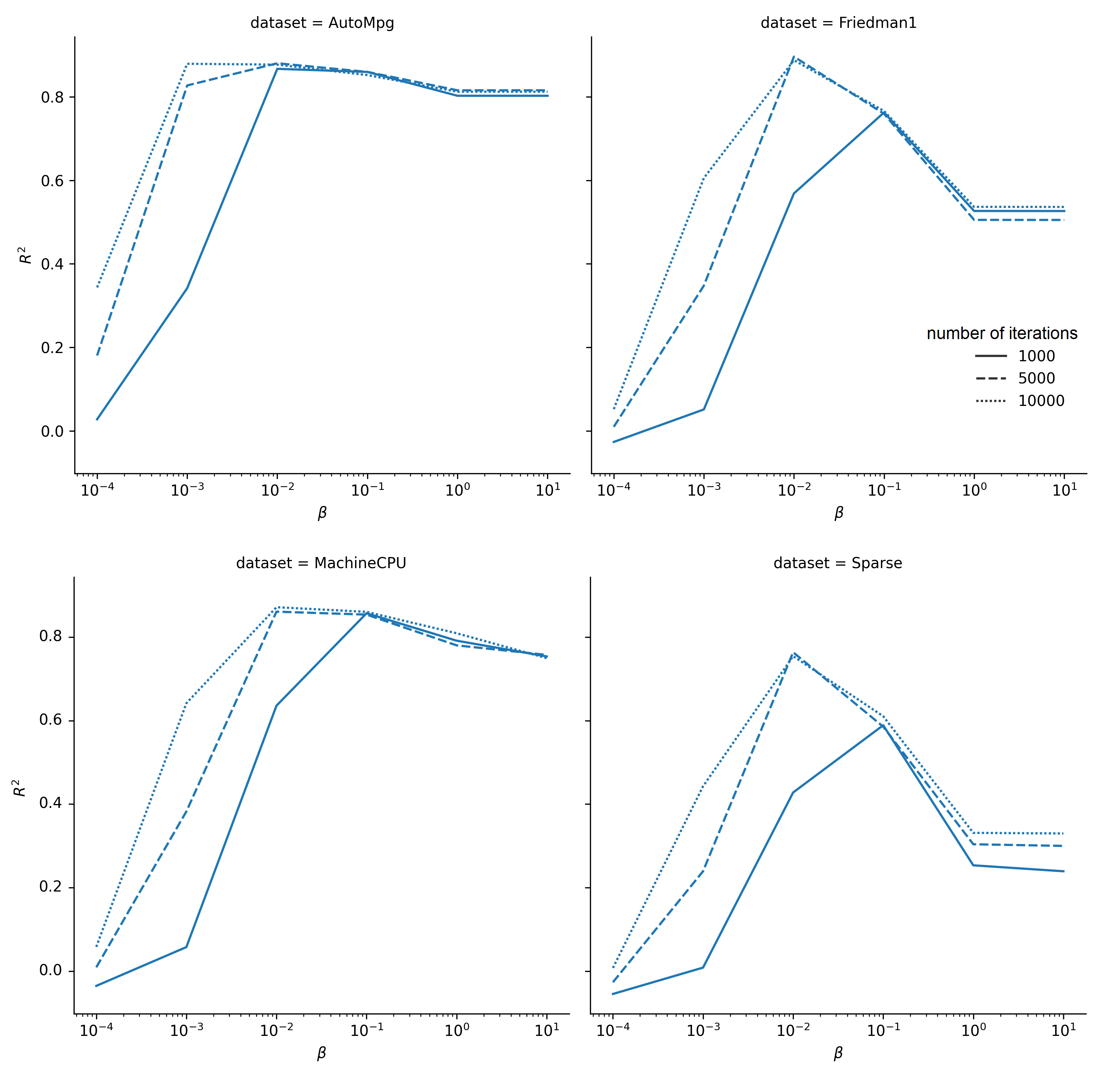
Figure 10: $R^{2}$ as a function of the regularization parameter $\beta$ for four datasets by different numbers $T=1000$, $5000$, $10000$ of iterations

8.2 Classification

To study the proposed GBM-HRBM for solving classification problems, we apply datasets which are taken from the UCI Machine Learning Repository [78], in particular, Balance Scale (Balance), Car Evaluation (Car), Dermatology, Diabetic Retinopathy (Retinopathy), Glass Identification (Glass) Haberman’s Survival (Haberman), Ionosphere, Seeds, Seismic-Bumps (Seismic), Soybean, Teaching Assistant Evaluation (Teaching), Tic-Tac-Toe Endgame (TTT), Website Phishing (Website), Wholesale Customer (Wholesale). Short notations of datasets are given in brackets. The dataset Diabetes is taken from OpenML at https://www.openml.org/. Table 5 shows the number of features $d$ for the corresponding data set, the number of examples $N$, and the number of classes $C$. More detailed information can be found from the data resources. Parameters of experiments coincide with similar parameters in experiments with the regression models.

Table 5: A brief introduction about the classification data sets

Dataset	$d$	$N$	$C$	Dataset	$d$	$N$	$C$
Balance	$4$	$625$	$3$	Seeds	$7$	$210$	$3$
Car	$6$	$1728$	$4$	Seismic	$18$	$2584$	$2$
Dermatology	$33$	$366$	$6$	Soybean	$35$	$47$	$4$
Diabetes	$9$	$768$	$2$	TTT	$27$	$957$	$2$
Glass	$10$	$214$	$6$	Teaching	$5$	$151$	$3$
Haberman	$3$	$306$	$2$	Website	$9$	$1353$	$3$
Ionosphere	$34$	$351$	$2$	Wholesale	$6$	$440$	$3$
Retinopathy	$20$	$1151$	$2$

First, we compare values of $F_{1}$ obtained for GBM-HRBM with the best results provided by one of the models: RF, ERT, GBM. Results are shown in Table 6. The largest differences between values of $F_{1}$ are for datasets Balance ($\allowbreak 0.168\,$), Dermatology ($0.112$), Seismic ($\allowbreak 0.071\,$). For comparison, we again apply the $t$-test. The obtained p-value is $p=0.0066$. This implies that the outperformance of GBM-HRBM is statistically significant.

Table 6: $F1$ measures for comparison of different types of the RF, ERT, GBM, GBM-HRBM in the classification tasks

Dataset	RF	ERT	GBM	GBM-HRBM
Balance	$0.599$	$0.614$	$0.662$	$\mathbf{0.830}$
Car	$0.837$	$0.873$	$\mathbf{0.985}$	$0.968$
Dermatology	$0.201$	$0.191$	$0.196$	$\mathbf{0.313}$
Diabetes	$0.722$	$0.703$	$0.719$	$\mathbf{0.729}$
Glass	$0.683$	$0.602$	$0.658$	$\mathbf{0.697}$
Haberman	$0.514$	$0.439$	$0.487$	$\mathbf{0.594}$
Ionosphere	$0.926$	$\mathbf{0.934}$	$0.922$	$0.932$
Retinopathy	$0.677$	$0.690$	$0.694$	$\mathbf{0.719}$
Seeds	$0.928$	$0.929$	$0.929$	$\mathbf{0.940}$
Seismic	$0.484$	$0.483$	$0.490$	$\mathbf{0.561}$
Soybean	$0.989$	$0.990$	$0.961$	$\mathbf{1.000}$
TTT	$0.968$	$0.978$	$\mathbf{0.998}$	$0.996$
Teaching	$0.580$	$0.546$	$0.575$	$\mathbf{0.633}$
Website	$0.792$	$0.749$	$0.841$	$\mathbf{0.868}$
Wholesale	$0.278$	$0.278$	$0.278$	$\mathbf{0.342}$

In order to compare corners and rectangles as base models, we compute values of $F_{1}$ score for the classification datasets taking GBM-HRBM with corners and rectangles. The corresponding results are shown in Table 7. One can again see that corners provide outperforming results for most datasets. The application of the $t$-test shows that p-value in this case is equal to $p=0.031$. It implies that corners again give the statistically significant outperformance.

Table 7: $F1$ measures for comparison of classifiers with different types of rectangles: corners and closed rectangles

Dataset	Corners	Rectangles
Balance	$\mathbf{0.830}$	$0.803$
Car	$\mathbf{0.968}$	$0.955$
Dermatology	$\mathbf{0.313}$	$0.185$
Diabetes	$\mathbf{0.729}$	$0.725$
Glass	$\mathbf{0.697}$	$0.692$
Haberman	$0.591$	$\mathbf{0.594}$
Ionosphere	$\mathbf{0.932}$	$0.915$
Retinopathy	$\mathbf{0.719}$	$0.689$
Seeds	$\mathbf{0.940}$	$0.938$
Seismic	$\mathbf{0.561}$	$0.554$
Soybean	$\mathbf{1.000}$	$\mathbf{1.000}$
TTT	$\mathbf{0.996}$	$0.962$
Teaching	$\mathbf{0.633}$	$0.624$
Website	$\mathbf{0.868}$	$0.863$
Wholesale	$\mathbf{0.342}$	$0.323$

8.3 SHAP and GBM-HRBM

In order to study modifications of SHAP for GBM-HRBM, we use the regression dataset MachineCPU. Fig. 11 shows Shapley values $\phi_{i}$ of all features (MYCT, MMIN, MMAX, CACH, CHMIN, CHMAX) obtained by two methods: the data-based SHAP and the model-based SHAP. Four randomly selected examples from the dataset are used for comparison of methods. We do not provide Shapley values obtained by using the original SHAP because they totally coincide with the corresponding values provided by the data-based method. It follows from Fig. 11 that most Shapley values calculated by using the data-based SHAP are similar to the corresponding Shapley values calculated by using the model-based SHAP. It should be noted that there is some divergence of results. In particular, Shapley values of the feature CHMAX in the example 4 are quite different and even have different signs. However, this case can be regarded as an exception to the rule.

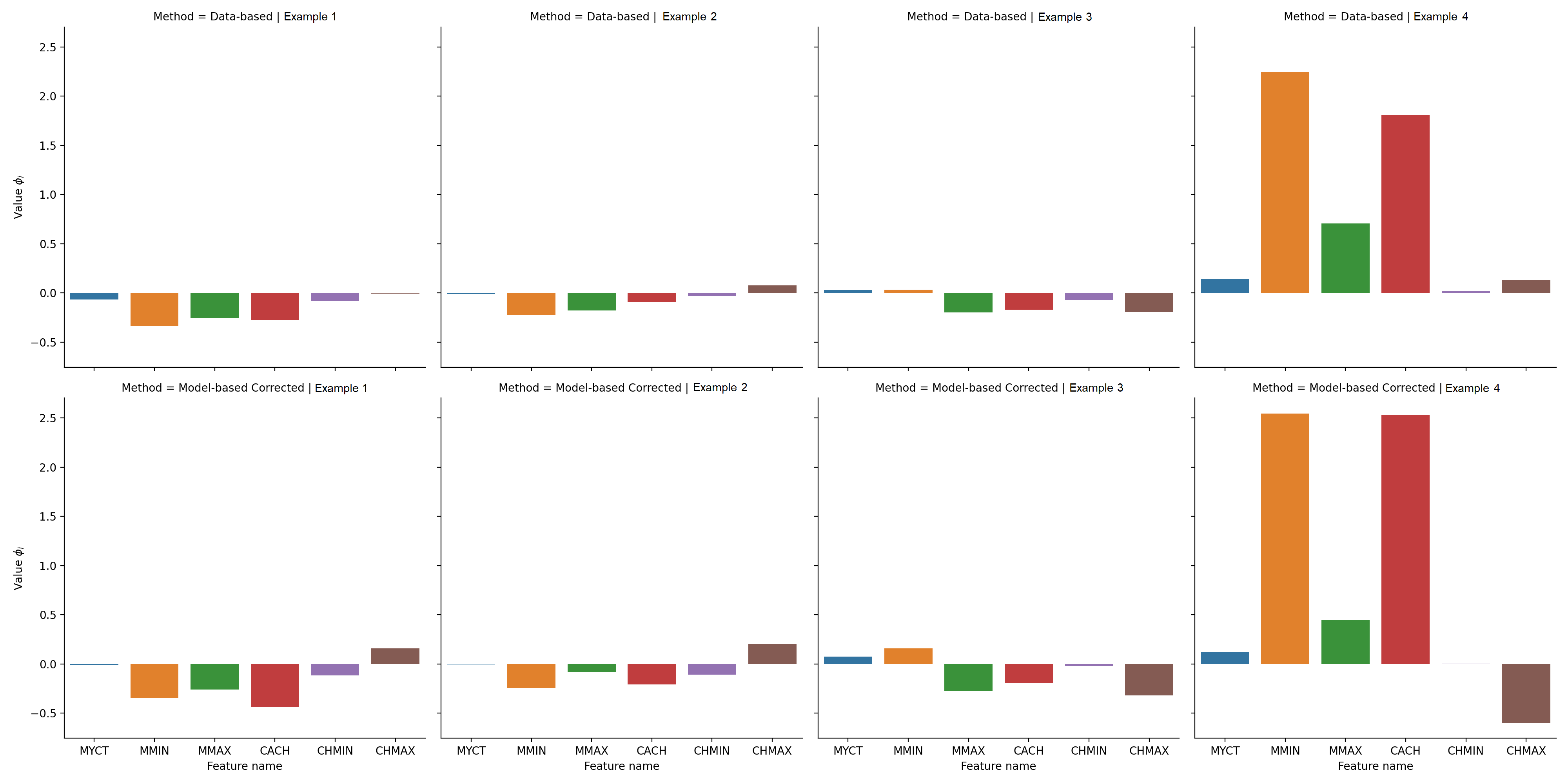
Figure 11: Comparison of Shapley values obtained by using the data-based SHAP (the first row of pictures) and the model-based SHAP (the second row of pictures) for the dataset MachineCPU

Fig. 12 depicts the violin plot of Shapley values for the same dataset MachineCPU. It can be viewed as a statistics of Shapley values for the whole dataset, including training and testing examples. One can see from the plot that the largest Shapley value corresponds to the feature MMAX. Moreover, we can conclude from Fig. 12 that the model-based SHAP and the data-based SHAP produce very similar Shapley values.

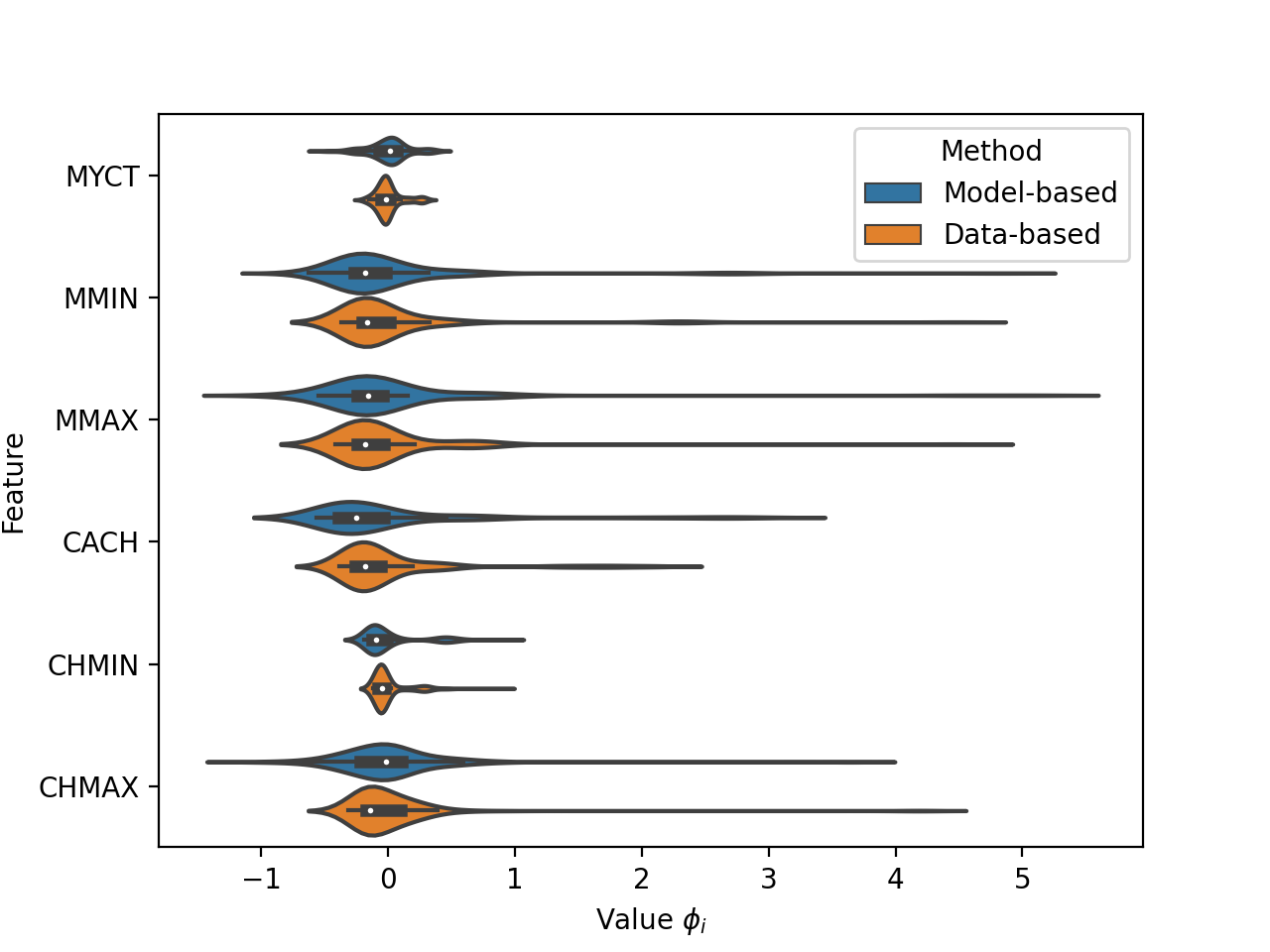
Figure 12: The violin plot of Shapley values obtained by using the data-based SHAP (the first row of pictures) and the model-based SHAP (the second row of pictures) for the dataset MachineCPU

Table 8 shows computational times in seconds for computing Shapley values of $n$ examples by using the original SHAP, the data-based SHAP, and the model-based SHAP. We use $10000$ iterations of GBM-HRBM under condition that corners are used as base models. It can be seen from Table 8 that computational time of the original SHAP linearly increases with $n$ whereas the proposed modifications of SHAP are changed very slowly.

Table 8: Computation time (seconds) of the original SHAP and two its GBM-HRBM modifications

	SHAP
$n$	Original	Data-based	Model-based
$1$	$2.780$	$0.874$	$0.071$
$10$	$27.130$	$0.990$	$0.073$
$20$	$54.087$	$1.062$	$0.075$

In order to see that the data-based and model-based SHAP models provide similar Shapley values, we consider the dataset Boston. Fig. 13 shows Shapley values $\phi_{i}$ of all features (CRIM, ZN, INDUS, CHAS, NOX, RM, AGE, DIS, RAD, TAX, PTRATIO, B, LSTAT), obtained by the same two methods. We again randomly select four examples from the dataset for analyzing. Fig. 14 depicts the violin plot of Shapley values for the dataset Boston. It can be seen from the plot that the largest Shapley value corresponds to features RM and LSTAT. It is interesting to note that the same features have been selected as the most important ones in [80].

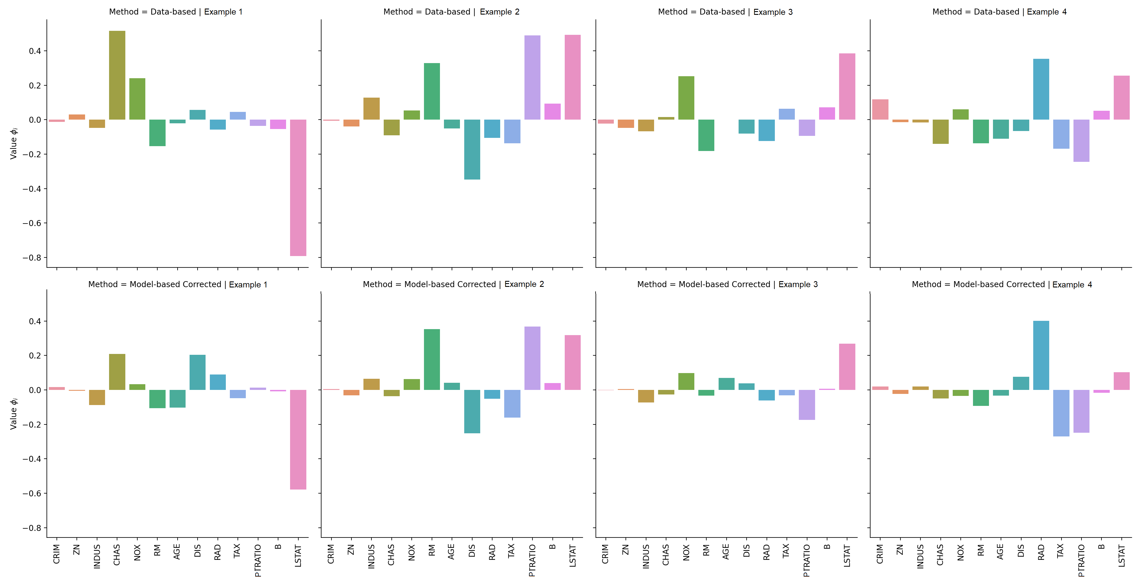
Figure 13: Comparison of Shapley values obtained by using the data-based SHAP (the first row of pictures) and the model-based SHAP (the second row of pictures) for the dataset Boston

Figure 14: The violin plot of Shapley values obtained by using the data-based SHAP (the first row of pictures) and the model-based SHAP (the second row of pictures) for the dataset Boston

9 Conclusion

A new ensemble model based on GBM with axis-parallel HRBMs as base models has been proposed. Two types of HRBMs have been studied: closed rectangles and corners. Numerical experiments have shown that corners mainly provide better results in comparison with closed rectangles. The proposed ensemble-based model is extremely simple due to simplicity of HRBMs. In spite of the model simplicity, various numerical experiments with real data have demonstrated the model efficiency and its overfitting prevention. If to compare HRBMs with decision trees, which are the most popular base models in boosting methods, then HRBM are much simpler than trees even with the minimal depth. At the same time, GBM-HRBM outperforms GBM with decision trees.

Another advantage of GBM-HRBM is that optimal parameters of regularization can be controlled at each iteration of GBM. This peculiarity of GBM-HRBM also improves the proposed ensemble-based model and reduces the computational time for training and testing the GBM-HRBM model.

A surprising peculiarity of the GBM-HRBM is that it is interpretable in a simple way by applying the SHAP interpretation method. We do not need to get a huge number of predictions for various subsets of features as it is performed in the original SHAP. Moreover, we do not need to use one of the available methods [81] for removing the features. Propositions 5 and 6 significantly simplify SHAP and provide accurate Shapley values.

It should be pointed out that HRBMs open a door for developing various modifications which could improve and simplify the regression and classification tasks. Therefore, several aspects of HRBMs will be covered in subsequent works. First, algorithms for generating optimal rectangles, for predicting and testing can be improved in order to reduce the computation time. Second, expectations (56) in the data-based modification of SHAP can be calculated through estimate of the probability density function based on the same rectangles by applying the well-known algorithms for the density estimation. This is an interesting direction for further research. Third, GBM-HRBM can be implemented as a simple and accurate interpretable approximating meta-model for complex black-box models. Fourth, it is interesting to study different algorithms to analyze training examples inside rectangles, for instance, to apply the attention mechanism to correct the mean target values of examples. It is expected that these algorithms will significantly improve the whole GBM with HRBMs.

Appendix A Appendix: Proof of Propositions

Proof of Proposition 1: If $\lambda_{1}=0$, then the extended loss function $\tilde{\mathcal{L}}$ in (30) has a minimum at a point with zero derivatives. This implies that there hold

$$\dfrac{\partial\tilde{\mathcal{L}}}{\partial v_{in}}=\dfrac{1}{N}\left(G_{in}+v_{in}H_{in}\right)+\lambda_{2}v_{in}=0,$$ (A.1)

$$\dfrac{\partial\tilde{\mathcal{L}}}{\partial v_{out}}=\dfrac{1}{N}\left(G_{out}+v_{out}H_{out}\right)+\lambda_{2}v_{out}=0.$$ (A.2)

Hence, we directly get (31). In the same way, the case when $\lambda_{1}>0$ and $\lambda_{2}>0$ can be considered. In this case, we have to take into account the sign of $v_{in}(\lambda_{1},\lambda_{2})$. Suppose that $v_{in}(\lambda_{1},\lambda_{2})>0$. Then we write

$$\dfrac{\partial\tilde{\mathcal{L}}}{\partial v_{in}}=\dfrac{1}{N}\left(G_{in}+v_{in}H_{in}\right)+\lambda_{2}v_{in}+\lambda_{1}=0.$$ (A.3)

Hence, there holds

$$v_{in}(\lambda_{1},\lambda_{2})=-\frac{G_{in}+N\cdot\lambda_{1}}{N\cdot\lambda_{2}+H_{in}}.$$ (A.4)

It follows from (A.4) that condition $v_{in}(\lambda_{1},\lambda_{2})>0$ is fulfilled when $G_{in}+N\cdot\lambda_{1}<0$ because the second derivative $h_{i}$ is positive. In the same way, we can get other cases for $v_{in}(\lambda_{1},\lambda_{2})$. Finally, we write (32). Similarly, we can find values of $v_{out}(\lambda_{1},\lambda_{2})$. $\blacksquare$

Proof of Proposition 2: Note that there holds

$$\frac{\partial\Omega_{h}}{\partial v_{in}}=-\frac{\partial\Omega_{h}}{\partial v_{out}}.$$ (A.5)

This implies that values of $v_{in}$ and $v_{out}$ are connected without a dependence of the regularization parameters ($\eta_{1},\eta_{2}$) because the following is valid:

$$0=\frac{\partial(\hat{L}+\Omega_{h})}{\partial v_{in}}+\frac{\partial(\hat{L}+\Omega_{h})}{\partial v_{out}}=\frac{\partial\hat{L}}{\partial v_{in}}+\frac{\partial\hat{L}}{\partial v_{out}}.$$ (A.6)

Hence, there holds

$$v_{out}=-\frac{G+v_{in}\cdot H_{in}}{H_{out}}.$$ (A.7)

If $\eta_{1}=0$, then we get (34). The value of $v_{out}(\eta_{2})$ can be obtained by substituting (34) into (A.7) and by taking into account that there hold $G=G_{in}+G_{out}$ and $H=H_{in}+H_{out}$.

If $\eta_{1}>0$ and $\eta_{2}=0$, then we obtain

$$v_{in}(\eta_{1})=\left\{\begin{array}[c]{cc}-\frac{G_{in}-N\cdot\eta_{1}}{H_{in}},&\frac{H_{in}G_{out}-H_{out}G_{in}}{H}<-N\cdot\eta_{1},\\ -\frac{G_{in}}{H_{in}},&\left|\frac{H_{in}G_{out}-H_{out}G_{in}}{H}\right|\leq N\cdot\eta_{1},\\ -\frac{G_{in}+N\cdot\eta_{1}}{H_{in}},&\frac{H_{in}G_{out}-H_{out}G_{in}}{H}>N\cdot\eta_{1}.\end{array}\right.$$ (A.8)

It should be noted that $v_{in}(\eta_{1})=-G_{in}/H_{in}$ as well as $v_{out}=-G_{out}/H_{out}$ do not depend on $\eta_{1}$ when $\left|\frac{H_{in}G_{out}-H_{out}G_{in}}{H}\right|\leq N\cdot\eta_{1}$. This implies that the regularization term is reduced to a constant. It is simply to show that other cases of the regularization can be implemented by using only the case $\eta_{2}>0$, $\eta_{1}=0$. $\blacksquare$

Proof of Proposition 3: If $\mathbb{I}_{in}^{(i)}=1$, i.e., there holds $\mathbf{x}_{i}\in\mathbf{r}$, then $\mathbb{I}_{out}^{(i)}=0$, and the condition (38) can be rewritten by using (22) as

$$\left|v_{in}\right|\leq\beta.$$ (A.9)

If we substitute (31) into (A.9), then the constraint for $v_{in}$ can be fulfilled by choosing the corresponding value of $\lambda_{2}$ in (30) denoted as $\lambda_{2}^{in}$:

$$\left|-\frac{G_{in}}{N\cdot\lambda_{2}^{in}+H_{in}}\right|\leq\beta.$$ (A.10)

The constraint for $v_{out}$ can be similarly written as follows:

$$\left|-\frac{G_{out}}{N\cdot\lambda_{2}^{out}+H_{out}}\right|\leq\beta.$$ (A.11)

Since the second derivative $h_{i}$ is positive for convex loss functions, then it follows from (A.10) that there holds:

$$\underline{\lambda}_{2}^{in}=\frac{1}{N}\left[\frac{1}{\beta}\left|G_{in}\right|-H_{in}\right].$$ (A.12)

Hence, the constraint (A.9) is fulfilled for all values $\lambda_{2}^{in}\geq\underline{\lambda}_{2}^{in}$. The same can be written for $\underline{\lambda}_{2}^{out}$. Hence, the maximum value of $\lambda_{2}$ defined as (39)

$$\lambda_{2}=\max\left({\underline{\lambda}_{2}^{in},\underline{\lambda}_{2}^{out},0}\right)$$ (A.13)

satisfies both constraints and therefore (38).

Similarly, we can get parameters for the $L_{1}$ regularization by writing the condition

$$\max\left(\left|\frac{G_{in}+N\cdot\lambda_{1}}{H_{in}}\right|,\left|\frac{G_{in}-N\cdot\lambda_{1}}{H_{in}}\right|\right)\leq\beta.$$ (A.14)

Hence, we obtain (42)-(44). $\blacksquare$

Proof of Proposition 4: First, we consider a case when $\mathbb{I}_{in}^{(i)}=1$ and $f_{k}(\mathbf{x})=v_{in}(\eta_{2})$. Then substituting (34) into (38) or (A.9), we get the condition:

$$|v_{in}(\eta_{2})|=\left|\frac{G_{in}+N\cdot\eta_{2}\cdot\left(\frac{G}{H_{out}}\right)}{H_{in}+N\cdot\eta_{2}\cdot\left(\frac{H}{H_{out}}\right)}\right|\leq\beta.$$ (A.15)

It can be rewritten as the following two inequalities:

$$-\beta\cdot\left(H_{in}+\eta_{2}\cdot N\cdot\left(\frac{H}{H_{out}}\right)\right)\leq G_{in}+\eta_{2}\cdot N\cdot\left(\frac{G}{H_{out}}\right),$$ (A.16)

$$\beta\cdot\left(H_{in}+\eta_{2}\cdot N\cdot\left(\frac{H}{H_{out}}\right)\right)\geq G_{in}+\eta_{2}\cdot N\cdot\left(\frac{G}{H_{out}}\right).$$ (A.17)

Hence, we get constraints for $\eta_{2}$:

$$\eta_{2}\cdot\left(G+\beta\cdot H\right)\geq\frac{H_{out}}{N}(G_{in}+\beta\cdot H_{in}),$$ (A.18)

$$\eta_{2}\cdot\left(G-\beta\cdot H\right)\leq-\frac{H_{out}}{N}(G_{in}+\beta\cdot H_{in}).$$ (A.19)

In order to find the minimal value $\eta_{2}$ which satisfies the above constraints, three cases should be considered: $G>\beta H$, $-\beta H<G<\beta H$, and $G<-\beta H$. Denote

$$C_{1}=\frac{H_{out}}{N}\frac{G_{in}+\beta H_{in}}{G+\beta H},\ C_{2}=-\frac{H_{out}}{N}\frac{G_{in}+\beta H_{in}}{G-\beta H}.$$ (A.20)

1. If $G>\beta H$, then it follows from (A.18) and (A.19) that $\eta_{2}\geq C_{1}$ and $\eta_{2}\leq C_{2}$. Hence, the smallest feasible solution for $\eta_{2}$ is $\underline{\eta}_{2}=C_{1}$ because the second inequality provides non-negative values of $\eta_{2}$.

2. If $|G|<\beta H$, then $\eta_{2}\geq C_{1}$ and $\eta_{2}\geq C_{2}$. Hence, the smallest feasible solution for $\eta_{2}$ is $\underline{\eta}_{2}=\max\left(C_{2}{,}C_{1}\right)$.

3. If $G<-\beta H$, then conditions for $\eta_{2}$ are $\eta_{2}\leq C_{1}$ and $\eta_{2}\geq C_{2}$. Hence, it is obvious that the smallest feasible solution for $\eta_{2}$ is $\underline{\eta}_{2}=C_{2}$.

Let us consider the second case when $\mathbb{I}_{out}^{(i)}=1$ and $f_{k}(\mathbf{x})=v_{out}(\eta_{2})$. Since the condition (38) has to be fulfilled for $v_{in}$ as well as for $v_{out}$, then the minimal value of $\eta_{2}$ depends on the same three cases. The corresponding bounds for $\eta_{2}$ can be obtained in the same way. $\blacksquare$

Proof of Proposition 5: Represent expression (53) in another form:

$$\Psi(S)=\prod_{j\in S}\mathbb{I}[x^{(j)}\in r^{(j)}]\cdot(v_{in}-v_{out})+v_{out}.$$ (A.21)

According to the fourth property of Shapley values (dummy), if the $j$-th feature falls in the $j$-th coordinate of the rectangle, i.e., $\mathbb{I}[x^{(j)}\in r^{(j)}]=1$, then its contribution is zero. Let the observation be inside the rectangle by means of the $i$-th feature, i.e., there holds

$$\mathbb{I}[x^{(i)}\in r^{(i)}]=1.$$ (A.22)

The above can be proved as follows. First, we can write

$$\Psi(S\cup\{i\}) =\mathbb{I}[x^{(i)}\in r^{(i)}]\cdot\prod_{j\in S}\mathbb{I}[x^{(j)}\in r^{(j)}]\cdot(v_{in}-v_{out})+v_{out}$$

$$=\Psi(S).$$ (A.23)

Hence, there holds

$$\phi_{i}=0.$$ (A.24)

For all other features, the second property (symmetry) holds in pairs. Indeed, if we write

$$\mathbb{I}[x^{(j)}\in r^{(j)}]=0,\ \mathbb{I}[x^{(k)}\in r^{(k)}]=0,$$ (A.25)

then the following is correct:

$$\Psi(S\cup\{j\})=v_{out}=\Psi(S\cup\{k\}).$$ (A.26)

Hence, there holds

$$\phi_{j}=\phi_{k}.$$ (A.27)

It follows from the first property (efficiency) that

$$\Psi(\{1,\dots,d\})=\Psi(\emptyset)+\sum_{i=1}^{d}\phi_{i}=\Psi(\emptyset)+\sum_{k=1}^{u}\tilde{\phi}=\Psi(\emptyset)+u\cdot\tilde{\phi},$$ (A.28)

where $u$ is the number of features for which the observation is outside $\mathbf{r}$; $\tilde{\phi}$ is a value of contribution for these features.

Then we get

$$\phi_{i}=\begin{cases}0,&x^{(i)}\in r^{(j)},\\ \dfrac{\Psi(\{1,\dots,d\})-\Psi(\emptyset)}{\sum_{j=1}^{d}\mathbb{I}[x^{(i)}\notin r^{(j)}]},&x^{(i)}\notin r^{(j)},\end{cases}$$ (A.29)

or, taking into account (A.21) and (54), we obtain (55), as was to be proved. $\blacksquare$

Proof of Proposition 6: Since the distribution of data is unknown, then the expectation of model predictions can be calculated by using some estimate of the density. Another way is to approximate the average over the sample. Due to simplicity, the second way is more preferable. Moreover, it does not introduce an additional error caused by a density estimation method. Hence, we write

$$\tilde{\Psi}(\emptyset)\approx v_{out}+(v_{in}-v_{out})\cdot\frac{1}{N}\sum_{t=1}^{N}\mathbb{I}[\mathbf{x}_{t}\in\mathbf{r}].$$ (A.30)

To calculate the subset function value, we have to estimate $\tilde{\Psi}(S)$ as

$$\tilde{\Psi}(S)\approx v_{out}+(v_{in}-v_{out})\cdot\mathbb{E}\left[\prod_{i=1}^{d}\mathbb{I}[X_{i}\in r^{(i)}]\mid X_{S}=\mathbf{x}^{(S)}\right],$$ (A.31)

where the expectation can be represented as:

$$\prod_{i\in S}\mathbb{I}[x_{i}\in r_{i}]\cdot\mathbb{E}\left[\prod_{i\notin S}\mathbb{I}[X_{i}\in r_{i}]\mid X_{S}=\mathbf{x}^{(S)}\right].$$ (A.32)

To estimate given expectations, the assumption is introduced [27, 28] that the feature random variables $S$ and $\overline{S}$ are independent. In this case, we can write

$$\mathbb{E}\left[\mathbb{I}[X_{\overline{S}}\in\mathbf{r}^{(\overline{S})}]\mid X_{S}=\mathbf{x}^{(S)}\right]$$

$$=\mathbb{E}_{X_{\overline{S}}}\left[\mathbb{I}[X_{\overline{S}}\in\mathbf{r}^{(\overline{S})}]\right]\approx\frac{1}{N}\sum_{t=1}^{N}\mathbb{I}[\mathbf{x}_{t}^{(\overline{S})}\in\mathbf{r}^{(\overline{S})}].$$ (A.33)

Thus, accepting a strong assumption about the independence of feature subsets, we finally get:

$$\tilde{\Psi}(S)=v_{out}+(v_{in}-v_{out})\mathbb{I}[\mathbf{x}^{(S)}\in\mathbf{r}^{(S)}]\cdot\frac{1}{N}\sum_{t=1}^{N}\mathbb{I}[\mathbf{x}_{t}^{(\overline{S})}\in\mathbf{r}^{(\overline{S})}].$$ (A.34)

Similarly to the first method (Proposition 5), we use the symmetry property. If (A.25) is valid, then there holds

$$\tilde{\Psi}(S\cup\{j\})=v_{out}=\tilde{\Psi}(S\cup\{k\}),$$ (A.35)

and, therefore, the equality $\phi_{j}=\phi_{k}=\widetilde{\phi}$ is valid. Otherwise, if the observation is inside the rectangle by feature $i$, then:

$$\tilde{\Psi}(S\cup\{i\}) =v_{out}+(v_{in}-v_{out})\cdot 1\cdot\mathbb{I}[\mathbf{x}^{(S)}\in\mathbf{r}^{(S)}]$$

$$\times\frac{1}{N}\sum_{t=1}^{N}\mathbb{I}[\mathbf{x}_{t}^{(\overline{S}\setminus\{i\})} \in\mathbf{r}^{(\overline{S}\setminus\{i\})}].$$ (A.36)

In sum, we get (58)-(60). $\blacksquare$

References

- [1] Xibin Dong, Zhiwen Yu, Wenming Cao, Yifan Shi, and Qianli Ma. A survey on ensemble learning. Frontiers of Computer Science, 14:241–258, 2020.
- [2] A.J. Ferreira and M.A.T. Figueiredo. Boosting algorithms: A review of methods, theory, and applications. In C. Zhang and Y. Ma, editors, Ensemble Machine Learning: Methods and Applications, pages 35–85. Springer, New York, 2012.
- [3] A. Jurek, Y. Bi, S. Wu, and C. Nugent. A survey of commonly used ensemble-based classification techniques. The Knowledge Engineering Review, 29(5):551–581, 2014.
- [4] J.M. Moreira, C. Soares, A.M. Jorge, and J.F.de Sousa. Ensemble approaches for regression: A survey. ACM Computing Surveys, 45(1):1–40, 2012.
- [5] M. Re and G. Valentini. Ensemble methods: a review. In Data Mining and Machine Learning for Astronomical Applications, Data Mining and Knowledge Discovery Series, chapter 26, pages 563–594. Chapman & Hall, 2012.
- [6] Y. Ren, L. Zhang, and P. N. Suganthan. Ensemble classification and regression-recent developments, applications and future directions [review article]. IEEE Computational Intelligence Magazine, 11(1):41–53, 2016.
- [7] L. Rokach. Ensemble-based classifiers. Artificial Intelligence Review, 33(1-2):1–39, 2010.
- [8] O. Sagi and L. Rokach. Ensemble learning: A survey. WIREs Data Mining and Knowledge Discovery, 8(e1249):1–18, 2018.
- [9] M. Wozniak, M. Grana, and E. Corchado. A survey of multiple classifier systems as hybrid systems. Information Fusion, pages 3–17, 2014.
- [10] Z.-H. Zhou. Ensemble Methods: Foundations and Algorithms. CRC Press, Boca Raton, 2012.
- [11] L. Breiman. Bagging predictors. Machine Learning, 24(2):123–140, 1996.
- [12] L. Breiman. Random forests. Machine learning, 45(1):5–32, 2001.
- [13] P. Geurts, D. Ernst, and L. Wehenkel. Extremely randomized trees. Machine learning, 63:3–42, 2006.
- [14] Y. Freund and R.E. Schapire. A decision theoretic generalization of on-line learning and an application to boosting. Journal of Computer and System Sciences, 55(1):119–139, 1997.
- [15] J.H. Friedman. Greedy function approximation: A gradient boosting machine. Annals of Statistics, 29:1189–1232, 2001.
- [16] J.H. Friedman. Stochastic gradient boosting. Computational statistics & data analysis, 38(4):367–378, 2002.
- [17] T. Chen and C. Guestrin. Xgboost: A scalable tree boosting system. In Proceedings of the 22nd ACM SIGKDD International Conference on Knowledge Discovery and Data Mining, pages 785–794, New York, NY, 2016. ACM.
- [18] K. Guolin, M. Qi, F. Thomas, W. Taifeng, C. Wei, M. Weidong, Y. Qiwei, and L. Tie-Yan. Lightgbm: A highly efficient gradient boosting decision tree. In Proceedings of the 31st International Conference on Neural Information Processing Systems (NIPS’17)), pages 3149–3157, 2017.
- [19] A.V. Dorogush, V. Ershov, and A. Gulin. Catboost: gradient boosting with categorical features support. arXiv:1810.11363, October 2018.
- [20] A. Natekin and A. Knoll. Gradient boosting machines, a tutorial. Frontiers in neurorobotics, 7(Article 21):1–21, 2013.
- [21] Wenxin Jiang. On weak base hypotheses and their implications for boosting regression and classification. The Annals of Statistics, 30(1):51–73, 2002.
- [22] P. Buhlmann and T. Hothorn. Boosting algorithms: Regularization, prediction and model fitting. Statistical Science, 22(4):477–505, 2007.
- [23] P. Buhlmann. Boosting for high-dimensional linear models. The Annals of Statistics, 34(2):559–583, 2006.
- [24] M. Schmid and T. Hothorn. Boosting additive models using component-wise p-splines. Computational Statistics & Data Analysis, 53(2):298–311, 2008.
- [25] T.G. Dietterich, T.D.A. Ashenfelter, and Y. Bulatov. Training conditional random fields via gradient tree boosting. In Proceedings of the 21st International Conference on Machine Learning (ICML), pages 1–8, 2004.
- [26] P. Viola and M. Jones. Rapid object detection using a boosted cascade of simple features. In Proceedings of the 2001 IEEE Computer Society Conference on Computer Vision and Pattern Recognition, CVPR 2001, pages 511–518. IEEE, 2001.
- [27] S.M. Lundberg and S.-I. Lee. A unified approach to interpreting model predictions. In Advances in Neural Information Processing Systems, pages 4765–4774, 2017.
- [28] E. Strumbelj and I. Kononenko. An efficient explanation of individual classifications using game theory. Journal of Machine Learning Research, 11:1–18, 2010.
- [29] L.S. Shapley. A value for n-person games. In Contributions to the Theory of Games, volume II of Annals of Mathematics Studies 28, pages 307–317. Princeton University Press, Princeton, 1953.
- [30] L.I. Kuncheva. Combining Pattern Classifiers: Methods and Algorithms. Wiley-Interscience, New Jersey, 2004.
- [31] I.D. Mienye and Yanxia Sun. A survey of ensemble learning: Concepts, algorithms, applications, and prospects. IEEE Access, 10:99129–99149, 2022.
- [32] L. Rokach. Ensemble Learning: Pattern Classification Using Ensemble Methods, volume 85. World Scientific, 2019.
- [33] C. Bentejac, A. Csorgo, and G. Martinez-Munoz. A comparative analysis of gradient boosting algorithms. Artificial Intelligence Review, 54:1937–1967, 2021.
- [34] J.T. Hancock and T.M. Khoshgoftaar. Catboost for big data: an interdisciplinary review. Journal of Big Data, 7(94):1–45, 2020.
- [35] Zhiyuan He, Danchen Lin, Thomas Lau, and Mike Wu. Gradient boosting machine: a survey. arXiv:1908.06951, Aug 2019.
- [36] A. Mayr, H. Binder, O. Gefeller, and M. Schmid. The evolution of boosting algorithms. Methods of information in medicine, 53(6):419–427, 2014.
- [37] S.M. Lundberg, G. Erion, H. Chen, A. DeGrave, J.M. Prutkin, B. Nair, R. Katz, J. Himmelfarb, N. Bansal, and S.-I. Lee. From local explanations to global understanding with explainable AI for trees. Nature Machine Intelligence, 2:56–67, 2020.
- [38] A.V. Konstantinov and L.V. Utkin. A generalized stacking for implementing ensembles of gradient boosting machines. In Cyber-Physical Systems, volume 350 of Studies in Systems, Decision and Control, pages 3–16. Springer, Cham, 2021.
- [39] M.T. Ribeiro, S. Singh, and C. Guestrin. “Why should I trust You?” Explaining the predictions of any classifier. arXiv:1602.04938v3, Aug 2016.
- [40] D. Garreau and U. von Luxburg. Looking deeper into tabular LIME. arXiv:2008.11092, August 2020.
- [41] Q. Huang, M. Yamada, Y. Tian, D. Singh, D. Yin, and Y. Chang. GraphLIME: Local interpretable model explanations for graph neural networks. arXiv:2001.06216, January 2020.
- [42] M.S. Kovalev, L.V. Utkin, and E.M. Kasimov. SurvLIME: A method for explaining machine learning survival models. Knowledge-Based Systems, 203:106164, 2020.
- [43] J. Rabold, H. Deininger, M. Siebers, and U. Schmid. Enriching visual with verbal explanations for relational concepts: Combining LIME with Aleph. arXiv:1910.01837v1, October 2019.
- [44] M.T. Ribeiro, S. Singh, and C. Guestrin. Anchors: High-precision model-agnostic explanations. In AAAI Conference on Artificial Intelligence, pages 1527–1535, 2018.
- [45] G.V. den Broeck, A. Lykov, M. Schleich, and D. Suciu. On the tractability of SHAP explanations. arXiv:2009.08634v2, January 2021.
- [46] K. Aas, M. Jullum, and A. Loland. Explaining individual predictions when features are dependent: More accurate approximations to Shapley values. arXiv:1903.10464, Mar 2019.
- [47] L. Antwarg, R.M. Miller, B. Shapira, and L. Rokach. Explaining anomalies detected by autoencoders using SHAP. arXiv:1903.02407v2, June 2020.
- [48] T. Begley, T. Schwedes, C. Frye, and I. Feige. Explainability for fair machine learning. arXiv:2010.07389, Oct 2020.
- [49] J. Bento, P. Saleiro, A.F. Cruz, M.A.T. Figueiredo, and P. Bizarro. TimeSHAP: Explaining recurrent models through sequence perturbations. arXiv:2012.00073, November 2020.
- [50] L. Bouneder, Y. Leo, and A. Lachapelle. X-SHAP: towards multiplicative explainability of machine learning. arXiv:2006.04574, June 2020.
- [51] N. Takeishi. Shapley values of reconstruction errors of PCA for explaining anomaly detection. arXiv:1909.03495, September 2019.
- [52] H. Yuan, H. Yu, J. Wang, K. Li, and S. Ji. On explainability of graph neural networks via subgraph explorations. arXiv:2102.05152, February 2020.
- [53] Y. Bi, D. Xiang, Zongyuan Ge, F. Li, C. Jia, and J. Song. An interpretable prediction model for identifying N7-methylguanosine sites based on XGBoost and SHAP. Molecular Therapy: Nucleic Acids, 22:362–372, 2020.
- [54] S. Mangalathu, S.-H. Hwang, and J.-S. Jeon. Failure mode and effects analysis of RC members based on machinelearning-based SHapley Additive exPlanations (SHAP) approach. Engineering Structures, 219:110927 (1–10), 2020.
- [55] R. Rodriguez-Perez and J. Bajorath. Interpretation of machine learning models using shapley values: application to compound potency and multi-target activity predictions. Journal of Computer-Aided Molecular Design, 34:1013–1026, 2020.
- [56] C. Benard, G. Biau, S. Da Veiga, and E. Scornet. SHAFF: Fast and consistent SHApley eFfect estimates via random Forests. arXiv:2105.11724, May 2021.
- [57] C. Frye, D. de Mijolla, L. Cowton, M. Stanley, and I. Feige. Shapley-based explainability on the data manifold. arXiv:2006.01272, June 2020.
- [58] N. Jethani, M. Sudarshan, I. Covert, S.-I. Lee, and R. Ranganath. FastSHAP: Real-time shapley value estimation. arXiv:2107.07436, Jul 2021.
- [59] B. Rozemberczki and R. Sarkar. The shapley value of classifiers in ensemble games. arXiv:2101.02153, January 2021.
- [60] L.V. Utkin and A.V. Konstantinov. Ensembles of random shaps. Algorithms, 15(11):431, 2022.
- [61] V. Belle and I. Papantonis. Principles and practice of explainable machine learning. arXiv:2009.11698, September 2020.
- [62] R. Guidotti, A. Monreale, S. Ruggieri, F. Turini, F. Giannotti, and D. Pedreschi. A survey of methods for explaining black box models. ACM computing surveys, 51(5):93, 2019.
- [63] N. Xie, G. Ras, M. van Gerven, and D. Doran. Explainable deep learning: A field guide for the uninitiated. arXiv:2004.14545, April 2020.
- [64] A. Adadi and M. Berrada. Peeking inside the black-box: A survey on explainable artificial intelligence (XAI). IEEE Access, 6:52138–52160, 2018.
- [65] A.B. Arrieta, N. Diaz-Rodriguez, J. Del Ser, A. Bennetot, S. Tabik, A. Barbado, S. Garcia, S. Gil-Lopez, D. Molina, R. Benjamins, R. Chatila, and F. Herrera. Explainable artificial intelligence (XAI): Concepts, taxonomies, opportunities and challenges toward responsible AI. Information Fusion, 58:82–115, 2020.
- [66] D.V. Carvalho, E.M. Pereira, and J.S. Cardoso. Machine learning interpretability: A survey on methods and metrics. Electronics, 8(832):1–34, 2019.
- [67] A. Das and P. Rad. Opportunities and challenges in explainableartificial intelligence (XAI): A survey. arXiv:2006.11371v2, June 2020.
- [68] C. Rudin. Stop explaining black box machine learning models for high stakes decisions and use interpretable models instead. Nature Machine Intelligence, 1:206–215, 2019.
- [69] S.I. Amoukou, T. Salaun, and N. Brunel. Accurate shapley values for explaining tree-based models. In International Conference on Artificial Intelligence and Statistics, pages 2448–2465. PMLR, 2022.
- [70] A. Delgado-Panadero, B. Hernandez-Lorca, M.T. Garcia-Ordas, and J.A. Benitez-Andrades. Implementing local-explainability in gradient boosting trees: Feature contribution. Information Sciences, 589:199–212, 2022.
- [71] K. Futagami, Y. Fukazawa, N. Kapoor, and T. Kito. Pairwise acquisition prediction with SHAP value interpretation. The Journal of Finance and Data Science, 7:22–44, 2021.
- [72] M. Loecher, Dingyi Lai, and Wu Qi. Approximation of SHAP values for randomized tree ensembles. In Machine Learning and Knowledge Extraction. CD-MAKE 2022, volume 13480 of LNCS, pages 19–30. Springer, Cham, 2022.
- [73] S.M. Lundberg, G.G. Erion, and Su-In Lee. Consistent individualized feature attribution for tree ensembles. arXiv:1802.03888, Feb 2018.
- [74] M. Mayer. Shap for additively modeled features in a boosted trees model. arXiv:2207.14490, Jul 2022.
- [75] Qingyao Sun. Individualized and global feature attributions for gradient boosted trees in the presence of l2 regularization. arXiv:2211.04409, Nov 2022.
- [76] G. Di Teodoro, M. Monaci, and L. Palagi. Unboxing tree ensembles for interpretability: a hierarchical visualization tool and a multivariate optimal re-built tree. arXiv:2302.07580, Feb 2023.
- [77] J. Wang, L. Gou, W. Zhang, H. Yang, and H.W. Shen. DeepVID: Deep visual interpretation and diagnosis for image classifiers via knowledge distillation. IEEE Transactions on Visualization and Computer Graphics, 25(6):2168–2180, 2019.
- [78] D. Dua and C. Graff. UCI machine learning repository, 2017.
- [79] J. Demsar. Statistical comparisons of classifiers over multiple data sets. Journal of Machine Learning Research, 7:1–30, 2006.
- [80] A.V. Konstantinov and L.V. Utkin. Interpretable machine learning with an ensemble of gradient boosting machines. Knowledge-Based Systems, 222(106993):1–16, 2021.
- [81] I.C. Covert, S. Lundberg, and Su-In Lee. Explaining by removing: A unified framework for model explanation. Journal of Machine Learning Research, 22(1):9477–9566, 2021.