Wilson matrix kernel for lattice QCD on A64FX architecture

Abstract.

We study the implementation of the even-odd Wilson fermion matrix for lattice QCD simulations on the A64FX architecture. Efficient coding of the stencil operation is investigated for two-dimensional packing to SIMD vectors. We measure the sustained performance on the supercomputer Fugaku at RIKEN R-CCS and show the profiler result of our code, which may signal an unexpected source of slow-down in addition to the detailed efficiency of each part of the code.

1. Introduction

Lattice QCD has been one of the typical benchmark applications in high performance computing, in particular on massively parallel systems. It has been also the case for the post-K (supercomputer Fugaku) project in Japan. As one of the target applications of so-called Co-design project (Sato et al., 2020) in development of the A64FX architecture for Fugaku (Fujitsu, 2022), a high performance lattice QCD library has been developed and released as the “QCD Wide SIMD” (QWS) library (Ishikawa et al., 2023). The QWS library implements a linear equation solver, a typical bottleneck in lattice QCD simulations. It is a solver for the clover fermion matrix, which is one of the popular fermion operators. While QWS library achieves a good sustained performance of more than 100 PFlops, it has several restrictions: it implements only the clover fermion matrix, the site degree of freedom only in the $x$-direction is packed into a SIMD vector, and it requires specific parameter setups to achieve good performance. There is another general purpose lattice QCD code set “Bridge++” (Ueda et al., 2014; Bridge++ project, 2022) for which an optimized code branch for A64FX (Akahoshi et al., 2022) is being developed. This branch of Bridge++, named “QXS” after QWS, was originally developed as an interface to call the QWS library and thus the convention and data layout are the same as QWS. In addition, the QXS branch has implementation of several popular fermion matrices other than the clover fermion, while the above mentioned restrictions are relaxed in the QXS. In particular, the site degree of freedom in $x$-$y$ plane is packed into SIMD vectors, which is useful for practical simulations of lattice QCD. This generalization makes the shifts of field in $x$- and $y$-directions, that are necessary for the stencil calculation, more involved to retain sufficient performance.

In this paper, we focus on one of such fermion operators, the even-odd version of the Wilson fermion matrix, as a representative example of matrix that requires such stencil calculation. While A64FX shares the features of SIMD architecture with the same 512-bit length with the Intel AVX-512, different techniques are required to achieve sufficient arithmetic performance. It would be informative to summarize such tuning procedures for the stencil calculation on the A64FX architecture. We also address the experience of using a profiler to find out an unexpected source of performance decrease.

This paper is organized as follows. In the next section, we briefly summarize the target fermion matrix and related works. In Section 3, we describe our implementation of the Wilson fermion matrix on the A64FX architecture. Section 4 exhibits the performance measurement and profiling experience on the Fugaku system. The last section is devoted to summary and outlook.

2. Fermion matrix in lattice QCD

Quantum Chromodynamics (QCD) is the fundamental theory of the strong interaction among quarks and gluons. The lattice QCD is a field theory formulated on a Euclidean space-time lattice. The path integral quantization enables numerical simulations based on the Monte Carlo algorithm. In lattice QCD, the gauge field (gluons) is represented with $3\times 3$ complex matrix field, $U_{\mu}(x)\in SU(3)$, that is defined on links connecting site $x$ and neighboring site $x+\hat{\mu}$ where $\hat{\mu}$ is a unit vector along the $\mu$-th axis. Since the fermion fields, representing the quarks, are expressed as anti-commuting Grassmann numbers, they are integrated out and the result is a determinant of the fermion matrix $D$, which depends on the background gauge field. The determinant is evaluated as $\det D^{\dagger}D=\exp[-|D^{-1}\phi|^{2}]$, where $\dagger$ denotes hermitian conjugate and $\phi$ is a Gaussian noise vector. This requires one to compute $D^{-1}\phi$ during the Monte Carlo steps many times. In the standard Hybrid Monte Carlo algorithm widely used in lattice QCD simulations, one Monte Carlo step requires $O(10)$–$O(100)$ solving, in which $D$ is different for each solving as the background gauge field changes. In addition to the Hybrid Monte Carlo steps, calculation of an expectation value often requires $D^{-1}\phi^{\prime}$, where the right-hand side vector $\phi^{\prime}$ depends on the target quantity. In this way, solving linear equations of the form $D\psi=\phi$ is a major bottleneck of lattice QCD simulations. As $D$ is a large sparse matrix, iterative solver algorithms are applied to solve the linear equations, whose performance depends on the performance of multiplication of $D$.

Since the lattice QCD simulations are performed with finite lattice spacing, the final results are obtained after extrapolation to the continuum limit. The requirement for the fermion and gauge actions on the lattice is that they coincide with the continuum actions in the continuum limit, and thus their discretized forms including the fermion matrix $D$ are not unique. For the fermion action, several forms are used together with various improvements. In this paper, we focus on the Wilson fermion action, of which fermion matrix is denoted as $D_{\mathrm{W}}$ in the following. It is one of the most popular fermion actions and its improved version is the clover fermion implemented in QWS.

The Wilson fermion matrix is written as

$$D_{\mathrm{W}}(x,y)$$

(1) $$=\delta_{x,y}-\kappa\sum_{\mu=1}^{4}\left[(1-\gamma_{\mu})U_{\mu}(x)\delta_{x+\hat{\mu},y}+(1+\gamma_{\mu})U_{\mu}^{\dagger}(x-\hat{\mu})\delta_{x-\hat{\mu},y}\right],$$

where $x$, $y$ are lattice sites, $\gamma_{\mu}$ is a $4\times 4$ matrix acting on the spinor degree of freedom, $\kappa$ is a parameter related to the fermion mass $m$ as $\kappa=1/(8+2m)$. $U^{\dagger}_{\mu}$ is a Hermitian conjugate of $U_{\mu}$. $D_{\mathrm{W}}(x,y)$ contains only the coupling between neighboring sites as shown in Figure 1. Since the matrix $\gamma_{\mu}$ has only one nonzero element in each row and its value is $\pm 1$ or $\pm i$, its operation is essentially interchange of the components. Moreover, $\gamma_{\mu}$ satisfies $(\gamma_{\mu})^{2}=1$ so that the factor $(\gamma_{\mu}\pm 1)$ works as (two times) projection matrices. The four components of spinor ($\phi_{ia}$ with $i=1,\dots,4$) is decomposed into two sets of two-component spinors ($\phi^{(\pm)}_{ia}$ with $i=1,2$), to which the link variable $U_{\mu}(x)$ or $U_{\mu}^{\dagger}(x-\hat{\mu})$ is multiplied to the color degrees of freedom. After the link variable multiplication, one can easily reconstruct a four-component spinor. For illustration purpose, an example of serial version of pseudo code is listed in Fig. 2. Note that at lines 5 and 8 in the figure the right hand side vector is shifted with respect to the lattice sites to generate the left hand side for the stencil computation. The number of floating point operations is 1368 FLOP per lattice site and the B/F ratio is 1.12.

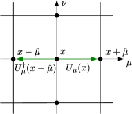
Figure 1. Schematic representation of the Wilson fermion matrix.

1:  for $x$ in sites do

2:     $\psi(x)=0$

3:     for $\mu$ in $x$-, $y$-, $z$-, $t$- directions do

4:        $\phi^{(+)}(x+\hat{\mu})={}$ two-component spinor made from$\allowbreak{(1+\gamma_{\mu})\phi(x+\hat{\mu})}$

5:        multiply $3\times 3$ link variables: $\phi^{(+)}(x):=U_{\mu}(x)\phi^{(+)}(x+\hat{\mu})$

6:        reconstruct four-component spinor from$\phi^{(+)}(x)$ and accumulate to $\psi(x)$

7:        $\phi^{(-)}(x-\hat{\mu})={}$ two-component spinor made from$\allowbreak{(1-\gamma_{\mu})\phi(x-\hat{\mu})}$

8:        multiply $3\times 3$ link variables:  ${\phi^{(-)}(x):=U_{\mu}^{\dagger}(x-\hat{\mu})\phi^{(-)}(x-\hat{\mu})}$

9:        reconstruct four-component spinor from$\phi^{(-)}(x)$ and accumulate to $\psi(x)$

10:     end for

11:  end for

Figure 2. Pseudo code of a serial version of Wilson fermion matrix operation: $\psi=D_{\mathrm{W}}\phi$.

The equation to be solved in lattice QCD simulations is

(2) $$\sum_{k}D_{\mathrm{W}}(j,k)\xi(k)=\eta(j),$$

where $\eta$ is a source vector, and $j$ and $k$ are collective indices of site, color, and spinor degrees of freedom. The even-odd preconditioning is frequently adopted to accelerate solving the above linear equation (2). Dividing the lattice sites into even and odd sites, Eq. (2) is equivalent to

(3) $$D_{\mathrm{W}}\begin{pmatrix}\xi_{\mathrm{e}}\\ \xi_{\mathrm{o}}\end{pmatrix}=\begin{pmatrix}D_{\mathrm{ee}}&D_{\mathrm{eo}}\\ D_{\mathrm{oe}}&D_{\mathrm{oo}}\\ \end{pmatrix}\begin{pmatrix}\xi_{\mathrm{e}}\\ \xi_{\mathrm{o}}\end{pmatrix}=\begin{pmatrix}\eta_{\mathrm{e}}\\ \eta_{\mathrm{o}}\end{pmatrix}.$$

Now $\xi_{\mathrm{e}}$ can be solved independently as in

(4) $$\left(1-D_{\mathrm{ee}}^{-1}D_{\mathrm{eo}}D_{\mathrm{oo}}^{-1}D_{\mathrm{oe}}\right)\xi_{\mathrm{e}}=D_{\mathrm{ee}}^{-1}\left(\eta_{\mathrm{e}}-D_{\mathrm{eo}}D_{\mathrm{oo}}^{-1}\eta_{\mathrm{o}}\right),$$

and from that, $\xi_{\mathrm{o}}$ is obtained as

(5) $$\xi_{\mathrm{o}}=D_{\mathrm{oo}}^{-1}\left(\eta_{\mathrm{o}}-D_{\mathrm{oe}}\xi_{\mathrm{e}}\right).$$

In the case of the Wilson fermion matrix, the diagonal blocks $D_{\mathrm{ee}}$ and $D_{\mathrm{oo}}$ are just unit matrices and their inverse is trivial. Arithmetic operations of $D_{\mathrm{eo}}$ and $D_{\mathrm{oe}}$ are in total the same as that of original $D_{\mathrm{W}}$. However, the operator on the left hand side of Eq. (4) has, in most cases, a smaller condition number than the original matrix $D_{\mathrm{W}}$, and thus it accelerates the solver algorithm. In addition, the working vectors in iterative linear equation solver requires half the size of full vectors, which has an advantage in memory access.

Here we briefly mention the related works on the tuning of lattice QCD simulation codes on the A64FX architecture. The situation just after the start of the shared use of supercomputer Fugaku was reviewed by Y. Nakamura at the symposium on lattice field theory in 2021 (Lattice2021) (Nakamura, 2021). The QWS library is a product of co-design project in the development of Fugaku, and achieves sustained performance of more than 100 PFlops (Ishikawa et al., 2023). It is a linear equation solver for clover fermion matrix and its implementation uses the Schwarz Alternating Procedure which accelerates the iterative solver by domain-decomposed matrix that reduces communication among the MPI processes. To achieve the above high performance, the local lattice volume is chosen so that the data are on L2 cache. The Bridge++ code set, the basis of this work, has developed various fermion matrices (Akahoshi et al., 2022). In particular, the five-dimensional formulation of the chirally improved fermion action (domain-wall fermion) was also conducted in the co-design project. Combining the Bridge++ and QWS library, the multi-grid solver for the clover fermion matrix is developed (Ishikawa et al., 2022). One of the widely used lattice QCD libraries, Grid, has also implemented the tuned code for A64FX architecture. The result on QPACE 4 (an FX700 system) was reported in Lattice 2021 (Meyer et al., 2022).

3. Implementation

3.1. SIMD features of A64FX architecture

The A64FX architecture is based on the Armv8.2-A instruction sets with the Scalable Vector Extension (SVE). The A64FX processor consists of 48 compute cores and 2 or 4 assistant cores, and 32 GiB on-package HBM memory. These cores and memory are grouped into four Core Memory Groups (CMGs), each having 12 compute cores sharing L2 cache of 8 MiB. The peak performance depends on the operating frequency mode, 2.0 GHz (normal mode) and 2.2 GHz (boost mode), and for the former the peak performance of floating-point number operations is 3.072 and 6.144 TFlops for double and single precision, respectively. The peak memory bandwidth per processor is 1024 GB/s.

Each node of Fugaku is composed of one A64FX processor, which is connected to a Tofu interconnect D (TofuD) network. TofuD network has a six-dimensional mesh-torus topology, whose bandwidth amounts to 28 Gbps $\times$ 2 lanes $\times$ 10 ports. In total, Fugaku has 158,976 nodes which correspond to 488 PFlops of peak performance for double precision in the normal mode.

The A64FX architecture has SIMD registers and operation units of 512-bit length. While the SIMD length is the same as Intel AVX-512 instruction set, prescription of optimization may differ significantly (for our implementation and obtained performance on the latter, see Ref. (Kanamori and Matsufuru, 2018)). One reason is that SIMD vector data types in Arm-SVE are sizeless, and the SIMD length incorporated in the instruction set architecture can take a range from 128- to 2048-bit. We thus cannot declare an array of such a SIMD data type.

Manual manipulation of SIMD the instructions is possible employing the Arm C Language Extension (ACLE) that is provided through intrinsics. Each intrinsic function directly specifies a SIMD operation on SIMD variables. Each vector instruction is accompanied by a predicate, that masks the operation on the elements in the SIMD vectors.

Another difference in implementations of Arm-SVE and AVX-512 is in the treatment of complex numbers. Compared to the latter, support of complex arithmetic operations inside a SIMD vector is insufficient for Arm-SVE. Such instructions, e.g. fcmla that provides a mixed operation for real and imaginary parts in a single SIMD vector, were installed rather a late stage of development and are slow due to its micro-code implementation (Fujitsu, 2022) .

The instruction for floating point arithmetics is rather straightforward. Here we list the instructions used in the following description for the shift of field in the form of intrinsic functions. For details of their operations are described in (ARM, 2020).

• LD1: basic load instruction to a SIMD vector register. In addition to the scalar base load instruction svld1, there are “gather-load” instructions in which the indices of the memory address are specified by a supplemental integer vector.

• ST1: basic store instruction from a SIMD vector to memory. Similarly to LD1, in addition to base store instruction svst1, there are “scatter-store” instructions in which the memory addresses are specified by an integer vector.

• SEL: this instruction selects elements from two vectors according to a given predicate; from the first vector for active predicate bits and from the second for inactive bits.

• TBL: arbitrary permutation of a given source vector according to an integer index vector. In a pseudo-code, it is like dst[i] = src[idx[i]].

• EXT: this instruction extracts consecutive elements of vector length from connected two vectors according to a given immediate integer value that specifies the head of the destination vector in the first source vector (cf. Figure 6). There is a similar instruction “SPLICE” that accompanies a predicate. It extracts $n$ contiguous elements from one source vector according to the predicate, shifts another source vector for upward $n$ elements, and merges them.

• COMPACT: this instruction collects active elements in a vector according to a predicate into lower consecutive elements of the vector and fills remaining elements with zero.

3.2. Data layout

The QWS library adopts packing the real and imaginary components of a complex value into separate SIMD vectors, due to the feature of arithmetic operations on complex numbers explained above. We follow the SIMD packing strategy of QWS and also adopt packing the site degree of freedom into SIMD vector. However, QWS packs the sites only in the $x$-direction into a single SIMD vector, that restricts the local lattice extent in the $x$-direction to be a multiple of the vector length, i.e. 8 in double and 16 in single precision cases. Moreover, these numbers are doubled for the even-odd matrix. This restriction is practically inconvenient. In the QXS branch of Bridge++, we thus decided to enable 2D SIMD packing in $x$-$y$ plane, as displayed in Figure 3. Except for this extension, the data layout of QXS follows the implementation of QWS.

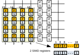
Figure 3. SIMD packing for the A64FX architecture in the case of $4\times 4$ $x$-$y$ tiling for single precision. Real and imaginary parts of the complex numbers are stored in separate SIMD vectors.

The above SIMD packing procedure leads to the following data layout. For the even-odd site index and single precision, the structure of the gauge and spinor fields read

float spinor[NT][NZ][NY/VLENY][NX/NEO/VLENX]

(6)                         [NC][ND][2][VLEN];

float gauge[NDIM][NEO][NT][NZ][NY/VLENY]

(7)                   [NX/NEO/VLENX][NC][NC][2][VLEN];

where $\text{{NC}}=3$ for colors, $\text{{ND}}=4$ for Dirac spinors, $\text{{NDIM}}=4$ for spacetime dimension, $\text{{NEO}}=2$ for even-odd, NX, NY, NZ, NT are the local lattice sizes in $x$, $y$, $z$, $t$-directions, [2] for real and imaginary components, $\text{{VLEN}}=16$ (SIMD vector length), and VLENX and VLENY are chosen so that $\text{{VLEN}}=\text{{VLENX}}\times\text{{VLENY}}$ ($\text{{VLENX}}\geq 2$). These values are set as preprocessor macro constants except for the local lattice sizes. This data layout is a straightforward extension of the layout of QWS to the $x$-$y$ SIMD tiling. Regarding the complex, color, and spinor degrees of freedom as a structure, the above layouts correspond to so-called “Array of Structure of array (AoSoA)”.

Storing the real and complex parts of complex numbers to separate SIMD registers makes a contrast to our implementation for Intel AVX-512 architecture (Kanamori and Matsufuru, 2018), in which the real and complex parts are stored contiguously in a single vector. Intel AVX-512 provides efficient complex operations for the elements of a SIMD vector. As a result, the number of sites packed into each vector is halved so that a 1D data layout is adopted where VLEN/2 sites in $x$-direction construct each SIMD vector.

3.3. Even-odd method

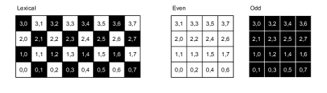
Figure 4. Left: Even and odd elements in an $x$-$y$ plane in a lexical form. White and black cells indicate even and odd elements, respectively, when the summation of the $z$ and $t$ indices is even. The numbers indicate the coordinates in $(y,x)$ form. Right: The even and odd elements are stored in separate arrays by compacting in the $x$-direction.

While the above $x$-$y$ SIMD packing largely relaxes the restriction on the local volume, the shift of field in $x$- and $y$-directions becomes somehow involved, in particular for the even-odd version of fermion matrix. Figure 4 explains the situation in the case of $4\times 4$ SIMD packing for single precision. The left panel shows the original lexical site index in the $x$-$y$ plane with colors according to the site being even (white) or odd (black) when the summation of the $z$ and $t$ indices is even. The assigned numbers represent $(y,x)$ coordinate values. The block matrices $D_{\mathrm{oe}}$ and $D_{\mathrm{eo}}$ act respectively on the even and odd vectors whose components are stored in separate arrays, as displayed in the right panel. For example, $D_{\mathrm{oe}}$ is multiplied with an even vector and results in an odd vector. In more detail, the function representing $D_{\mathrm{oe}}$ reads the data of an even vector, then apply eight points stencil operations expressed in Eq. (1), and write the result to an odd vector. $D_{\mathrm{eo}}$ plays a similar role for odd and even vectors, and for the Wilson fermion matrix $D_{\mathrm{ee}}$ and $D_{\mathrm{oo}}$ correspond to the multiplication of a unit matrix. In the case of the clover fermion matrix, implemented in QWS library as well as in Bridge++, $D_{\mathrm{ee}}$ and $D_{\mathrm{oo}}$ are site-local block diagonal operations.

3.4. Stencil access

A stencil operation on a structured lattice, in general, requires data on neighboring sites. If the site is not in local but in another process, the data are transferred with message passing. In our case, collecting the data on neighbor sites in $x$- and $y$-directions requires merging of two SIMD vectors into one vector even in a bulk part. One possible way to perform this operation is to use the gather-load in loading the data from memory (see Subsection 3.1). While the loading of data specifying the memory address by an index vector is convenient, in practice, the gather-load (and scatter-store) is rather slow. An alternative procedure is to load the data in units of SIMD vector and rearrange them on registers exploiting the SVE instructions. In what follows we describe the latter procedure for the even-odd Wilson matrix.

Since $D_{\mathrm{eo}}$ and $D_{\mathrm{oe}}$ contain the nearest neighbor couplings, one needs to shift the field in $\pm\mu$-direction before multiplying $U_{\mu}(x)$ or after multiplying $U_{\mu}^{\dagger}(x-\hat{\mu})$. Let us explain in more detail exemplifying $X^{-}$ contribution (the second term in the square brackets in Eq. (1)) in $D_{\mathrm{oe}}$ in Figure 5. Here we assume $4\times 4$ SIMD tiling in the single precision case as an example, while we can choose other values of VLENX and VLENY. To shift the field in $+x$-direction, components from two SIMD vectors are necessary to be loaded to construct a single SIMD vector. According to the parity of $(y+z+t)$ coordinates, a part of the SIMD vector is shifted as in the left panel of Figure 5. For $D_{\mathrm{oe}}$, this operation acts on an even vector (left) to generate an odd vector (right). An $X^{-}$ operation requires access to the even arrays in irregular shape as indicated by light gray cells. We first load the current and left neighbor regions to two registers z1 and z2, respectively, and use the sel instruction to merge them. Then the data in the SIMD vector are rearranged with tbl instruction.

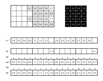
Figure 5. Shift of a field from the even array (top left) to the odd array (top right) in the stencil access of $D_{\mathrm{oe}}$. A $4\times 4$ square region corresponds to a SIMD register or an aligned memory space. An $X^{-}$ operation requires access to the even arrays in irregular shape as indicated by light gray cells. The contents of the SIMD register are shown in the lower part of the figure (ordered from left to right). z1, z2: Results of load instructions from the current and left neighbor of the even array. sel: Result of a sel instruction of z1 and z2 with a predicate register pg. tbl: Results of a tbl instruction which shuffles the previous result according to integer indices in another SIMD register idx.

The stencil access in $y$-direction is simpler than that in $x$-direction, as displayed in Figure 6 for $Y^{-}$ operation. We employ the ext instruction that extracts contiguous data from two SIMD vectors and stores in a single vector.

Figure 6. Similar to Fig. 5 but shift for $Y^{-}$ operation. An ext instruction with an immediate value 12 concatenates z1 and z2 and returns a shifted result.

3.5. Communication

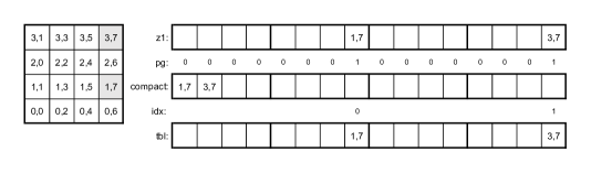
Figure 7. Packing and unpacking of data for MPI communications in the $X^{-}$ operation. Two of the sixteen elements in the SIMD register need to be sent. A compact instruction with a predicate indicating active elements collects them to the lower consecutive SIMD elements. After communication, the boundary data in the receive buffer are loaded to a SIMD vector and delivered to desired places by using the tbl instruction.

Since our code is parallelized with MPI, shifts of the SIMD elements in the $x$- and $y$-directions require communication with neighboring processes. For the communication, the boundary data are packed into the buffer array, sent to the neighbor process, and unpacked to merge with the data in the bulk region. The communications and the operations in bulk region are overlapped. Again communication in $x$-direction is involved as displayed in Figure 7. We first implemented these packing and unpacking processes with scatter-save and gather-load instructions with index vectors. However, for the aforementioned reason, we replace these steps with an alternative procedure as follows, which slightly increases the performance. After loading the boundary data into a SIMD vector, the compact instruction is used to compress them into lower elements of a temporal vector, that are stored into the buffer array. After the communication, the boundary data in the receive buffer are loaded to a SIMD vector and delivered to desired places by using the tbl instruction. The shift in $y$-direction is again simpler than $x$-direction because the boundary data are consecutive in a SIMD vector that are stored to buffer array using the standard store instruction with a predicate. Unpacking is implemented in a similar manner with a masked load instruction.

3.6. Multi-threading

In Fujitsu’s MPI libraries, the thread mode MPI_THREAD_MULTIPLE is not available, and thus communication is performed only by master thread under the MPI_THREAD_FUNNELED mode. Assuming that the assistant cores can execute background communication, the tasks are averagely assigned to all threads in the bulk part.

For the communication, boundary data are packed and unpacked before and after the bulk part. The packing of each direction is processed individually. The loop in each direction is over a three-dimensional boundary and averagely parallelized to the threads. This process is denoted “EO1” in this paper. Thus the load of each thread is well-balanced. On the other hand, for unpacking, denoted “EO2”, a single loop for all the local sites processes the unpacking of all the buffer data, since the number of boundaries concerning each site depends on the place of the site on local lattice. This causes load imbalance as we observe in the next section.

4. Performance benchmark

Performance is measured on the supercomputer Fugaku at RIKEN Center for Computational Science (R-CCS). We use a Fujitsu C/C++ compiler in its “clang mode” and the version of language and run-time is 4.8.1 tcsds-1.2.36. Unlike the “trad mode” adopted in QWS, clang mode supports several new features: full support of C++17, OpenMP 4.5, fp16 datatype, and ACLE for SVE. We set several compile-time and runtime options for optimal performance. The default value of the inline threshold in the clang mode turns out to be too small. To ensure that all eight hopping operations in the kernel function are expanded inline, we set -Rpass-missed=inline -mllvm -inline-threshold=1000 in addition to -Kfast as the compiler options. In the clang mode, the fast hardware barrier functionality within the 12 cores of a CMG is not enabled by default. To enable this feature, we set the environment variable FLIB_BARRIER =HARD whose impact to the performance amounts to about 20% at our smallest lattice size.

4.1. Profiler results

We measure cycle account information by using Fujitsu advanced performance profiler (FAPP). The target code is the kernels extracted from the version of Bridge++ QXS branch used in the presentation at Lattice 2022 symposium (Aoyama et al., 2023).

This profiling is performed on one node of A64FX processor running at 2.2 GHz. The total lattice size is $L_{x}\times L_{y}\times L_{z}\times L_{t}=16\times 16\times 16\times 16$, and the footprint of the gauge and spinor dataset is 18 MiB and 6 MiB, respectively. We use a standard combination of 4 MPI processes per node and 12 OpenMP threads per process. Assigning four processes to $[1,1,2,2]$ in parallelization, the local lattice size per process is $16\times 16\times 8\times 8$. Applying the $4\times 4$ SIMD tiling, each even/odd array consists of $2\times 4\times 8\times 8$ site elements. To emulate a situation of the weak-scaling test in the next subsection, we enforce the communication in $x$- and $y$-directions for the self MPI process.

Due to a small lattice size intending on-L2 computation, the execution period of each kernel function is short as $\lesssim 100$ $\mu$s. In this time scale, the overhead of APIs in the profiler becomes non-negligible. To mitigate this, we pass an option -Hmethod=fast for the measuring command fapp -C, which bypasses the operating system in reading hardware counters.

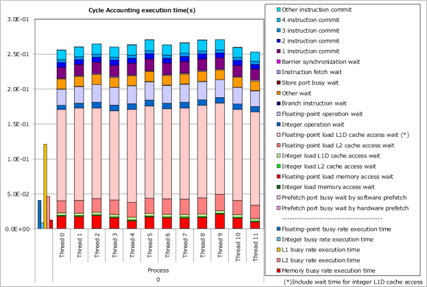
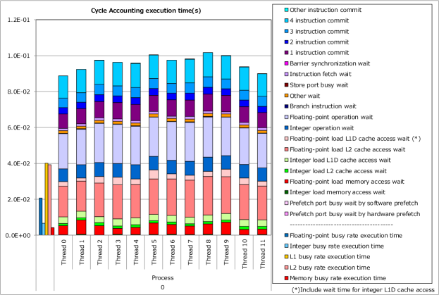
Figure 8. Cycle account information by FAPP: the initial result of the bulk part (top) and the result after tuning (bottom). The yellow bar on the leftmost column indicates the L1 cache busy time and pink colored parts in the twelve stacked bars are L1 cache wait time. The vertical axis shows the execution time in seconds after repeating the operation in Eq. (4) 1000 times. Note that the scales of the vertical axis are different in the two panels.

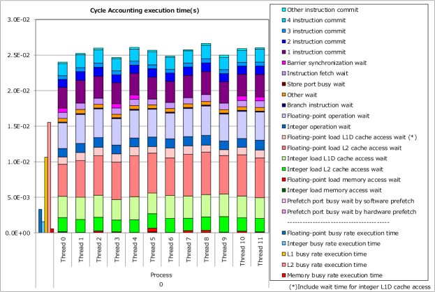
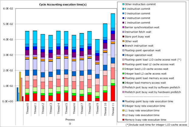
Figure 9. Cycle accounting information of the EO1 part for preparing the send buffer (top) and the EO2 part (bottom) for post-processing the received data.

Figure 8 shows the results of profiling the bulk part before and after the improvement. In the former case, heavy duty is imposed on the L1 cache resulting in a bottleneck of the entire kernel. This is an unexpected behavior regarding the property of a stencil kernel — it is usually memory or L2 bandwidth bottlenecked —. Careful examination of the profiler report reveals that some fraction of the load and store instructions was occupied by the gather-load and scatter-store instructions, even though no such ACLE intrinsic function is used in the code. It turned out that inefficient code was generated for the addition of accumulated result of the stencil operations to the destination array, and can be easily removed. This part was composed of nested two loops, inner for elements of a SIMD vector and outer for 24 (Re/Im)-spin-color degrees of freedom. Such structure is prepared for developing a portable prototype code expecting auto-vectorization by compilers for the inner loop. While optimization by ACLE was applied to replace them, such a code has remained in some parts of the code. Presumably, the compiler interchanged the outer and inner loops resulting in expensive stride accesses and gather-load/scatter-store instructions. Replacing this data structure with explicit SIMD intrinsics or collapsed single loop solves this pathological behavior. This fact implies that the clang mode of the Fujitsu compiler is not fully matured.

Figure 9 shows the profiling results of the EO1 kernel for preparing the send buffer and the EO2 kernel for post-processing the received data. Both the kernels contain multiplications of $3\times 3$ gauge field matrix for the data exported in upward directions and the data imported from the upward directions. Together with the bulk part in Figure 8, we find imbalance of execution time among the 12 threads, which is in particular sizable in EO2. This imbalance is also confirmed by the number of floating point operations executed on each core reported by the profiler. The reason for the imbalance is that the local lattice sites are uniformly distributed to 12 threads as mentioned in Section 3.6. When the lattice site is located on the boundary, some of the operations in the bulk part is reduced and moved to the EO1 and EO2 kernels. The load imbalance is significant in the EO2 kernel, in particular, in thread 11 because it processes more lattice sites on the boundary and some of them are involved in multiple directions. Especially, many of these sites receive the data from the upward process, which requires multiplication of $3\times 3$ gauge field matrix. In principle, the number of operations on each boundary lattice site can be statically evaluated in advance. In the future version, we plan to improve the load balance of the EO2 kernel based on this empirical information.

4.2. Performance of matrix multiplication

We measure the sustained performance of the even-odd Wilson matrix multiplication in the single precision case on the supercomputer Fugaku in normal mode (2.0 GHz). Throughout the performance measurements, we assign one MPI process to one CMG, i.e., four MPI processes are assigned to each node. In the following, each value of performance is measured in a single execution by multiplying the matrix to a vector 1000 times. Before the measurement, 300 seconds of sleep is inserted to avoid the possible effect of remaining I/O of the previous job caused by the file system of Fugaku.

The results of the sustained performance measured on a single node for lattice sizes $16\times 16\times 16\times 16$, $64\times 16\times 16\times 8$, and $64\times 32\times 32\times 16$ are summarized in Table 1. We vary the 2-dimensional shape of the SIMD tiling: $16\times 1$, $8\times 2$, $4\times 4$, and $2\times 8$. The MPI process assignment is $[1,1,2,2]$ in $(x,y,z,t)$ directions. The local lattice sizes for each process are listed in Table 1. As a part of the weak scaling measurement below, we enforce the communication in all four directions even when only one MPI process exists in that direction. For the smallest lattice, the data size is less than the L2 cache size, which explains its better performance than the larger lattices. There is no clear tendency against the shape of tiling, and the difference is not significant. Thus one can choose flexibly the values of VLENX and VLENY depending on the setup of lattice and node parameters.

In Figure 10, we show the weak scaling up to 512 nodes for the above three values of local lattice sizes, $16\times 16\times 8\times 8$, $64\times 16\times 8\times 4$, and $64\times 32\times 16\times 8$ with $4\times 4$ SIMD tiling. The same enforcement of communication is applied in the measurements. The rank maps are carefully prepared so that every neighboring communication can be made within the same node (between CMGs) or with a neighboring node in the 6-dimensional mesh-torus network topology. The performance per node is almost constant, implying very good scaling up to 512 nodes we measured. These local lattice sizes and numbers of nodes cover typical lattice sizes in practical simulations in these years.

For comparison, we also measure the performance of our code without ACLE implementation. It is implemented in the same manner except for employing an array of float of length VLEN instead of the builtin SIMD data type, svfloat32_t. The ACLE intrinsics are replaced with inline functions that play the same roles as the former. On a single node of Fugaku, this results in around 30 GFlops, about 10 times slower than the ACLE version, which implies the vectorization by the compiler is not properly applied in this case.

Table 1. Effect of the 2D tiling for the even-odd Wilson fermion matrix multiplication in single precision. The performance is measured with four MPI processes on a single node. The lattice volume in the left-most column is per process.

	$x$-$y$ tiling
lattice size/process	$16\times 1$	$8\times 2$	$4\times 4$	$2\times 8$
$16\times 16\times 8\times 8$	$-$	448	420	419
$64\times 16\times 8\times 4$	339	343	369	380
$64\times 32\times 16\times 8$	319	328	343	345	[GFlops]

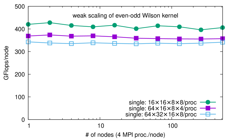
Figure 10. Weak scaling behavior of the sustained performance of the even-odd Wilson matrix multiplication in single precision on $16\times 16\times 8\times 8$, $64\times 16\times 8\times 4$, and $64\times 32\times 16\times 8$ local lattices per process.

5. Summary and outlook

This paper concerns our implementation of the even-odd Wilson fermion matrix for lattice QCD simulations on the A64FX architecture. Efficient coding of the stencil operation is investigated for two-dimensional packing to SIMD vectors. While the shifts of SIMD data in $x$- and $y$-directions are involved, in particular for the even-odd matrix, efficient implementation is achieved by exploiting the ACLE intrinsics to shuffle the elements of SIMD vectors instead of applying the gather-load and scatter-store instructions. We measured the sustained performance on the supercomputer Fugaku at RIKEN R-CCS as well as examined the result of profiling which sometimes signals unexpected sources of slow-down. The optimized code provides similar performance on other FX1000 systems, while adjustment of setup, such as environment variables may be necessary. These techniques are applicable to other fermion matrices in a straightforward way and also to other stencil calculations in general.

The $x$-$y$ tiling of the SIMD vector has been applied throughout the QXS branch of Bridge++. Tuning developed in this paper is now being applied to the other fermion matrices in the QXS branch. The code developed for the A64FX architecture will be made publicly available in the forthcoming release of Bridge++ version 2.0.

- (1)
- Akahoshi et al. (2022) Yutaro Akahoshi, Sinya Aoki, Tatsumi Aoyama, Issaku Kanamori, Kazuyuki Kanaya, Hideo Matsufuru, Yusuke Namekawa, Hidekatsu Nemura, and Yusuke Taniguchi. 2022. General purpose lattice QCD code set Bridge++ 2.0 for high performance computing. J. Phys. Conf. Ser. 2207, 1 (2022), 012053. https://doi.org/10.1088/1742-6596/2207/1/012053 arXiv:2111.04457 [hep-lat]
- Aoyama et al. (2023) Tatsumi Aoyama, Issaku Kanamori, Kazuyuki Kanaya, Hideo Matsufuru, and Yusuke Namekawa. 2023. Bridge++: Benchmark results on supercomputer Fugaku. PoS Lattice2022 (2023), 284, to appear.
- ARM (2020) ARM. 2015-2020. ARM C Language Extensions for SVE. https://developer.arm.com/documentation/100987/0000/.
- Bridge++ project (2022) Bridge++ project. 2012-2022. Lattice QCD code Bridge++. https://bridge.kek.jp/Lattice-code/.
- Fujitsu (2022) Fujitsu. 2022. A64FX. https://github.com/fujitsu/A64FX.
- Ishikawa et al. (2022) Ken-Ichi Ishikawa, Issaku Kanamori, and Hideo Matsufuru. 2022. Multigrid solver on Fugaku. PoS LATTICE2021 (2022), 278. https://doi.org/10.22323/1.396.0278 arXiv:2112.00501 [hep-lat]
- Ishikawa et al. (2023) Ken-Ichi Ishikawa, Issaku Kanamori, Hideo Matsufuru, Ikuo Miyoshi, Yuta Mukai, Yoshifumi Nakamura, Keigo Nitadori, and Miwako Tsuji. 2023. 102 PFLOPS lattice QCD quark solver on Fugaku. Comput. Phys. Commun. 282 (2023), 108510. https://doi.org/10.1016/j.cpc.2022.108510 arXiv:2109.10687 [hep-lat]
- Kanamori and Matsufuru (2018) Issaku Kanamori and Hideo Matsufuru. 2018. Practical Implementation of Lattice QCD Simulation on SIMD Machines with Intel AVX-512. Vol. 10962. Springer International Publishing, Cham, 456–471. https://doi.org/10.1007/978-3-319-95168-3_31 arXiv:1811.00893 [hep-lat]
- Meyer et al. (2022) Nils Meyer, Peter Georg, Stefan Solbrig, and Tilo Wettig. 2022. Grid on QPACE 4. PoS LATTICE2021 (2022), 068. https://doi.org/10.22323/1.396.0068 arXiv:2112.01852 [hep-lat]
- Nakamura (2021) Yoshifumi Nakamura. 2021. Software development and performance of Fugaku and ARM architectures. PoS LATTICE2021 (2021), 023. https://doi.org/10.22323/1.396.0023
- Sato et al. (2020) Mitsuhisa Sato, Yutaka Ishikawa, Hirofumi Tomita, Yuetsu Kodama, Tetsuya Odajima, Miwako Tsuji, Hisashi Yashiro, Masaki Aoki, Naoyuki Shida, Ikuo Miyoshi, Kouichi Hirai, Atsushi Furuya, Akira Asato, Kuniki Morita, and Toshiyuki Shimizu. 2020. Co-Design for A64FX Manycore Processor and ”Fugaku”. In Proceedings of the International Conference for High Performance Computing, Networking, ”Storage and Analysis (Atlanta, Georgia) (SC ’20). IEEE Press, Association for Computing MachineryNew YorkNYUnited States, Article 47, 15 pages.
- Ueda et al. (2014) S. Ueda, S. Aoki, T. Aoyama, K. Kanaya, H. Matsufuru, S. Motoki, Y. Namekawa, H. Nemura, Y. Taniguchi, and N. Ukita. 2014. Development of an object oriented lattice QCD code ‘Bridge++’. J. Phys. Conf. Ser. 523 (2014), 012046. https://doi.org/10.1088/1742-6596/523/1/012046