High-dimensional multi-view clustering methods

Abstract

Multi-view clustering has been widely used in recent years in comparison to single-view clustering, for clear reasons, as it offers more insights into the data, which has brought with it some challenges, such as how to combine these views or features. Most of recent work in this field focuses mainly on tensor representation instead of treating the data as simple matrices. This permits to deal with the high-order correlation between the data which the based matrix approach struggles to capture. Accordingly, we will examine and compare these approaches, particularly in two categories, namely graph-based clustering and subspace-based clustering. We will conduct and report experiments of the main clustering methods over a benchmark datasets.

Keywords Multi-view clustering  $\cdot$ Graph based Multi-view clustering  $\cdot$ Subspace based Multi-view clustering  $\cdot$ Tensor learning  $\cdot$ Representation learning

1 Introduction

Clustering (Li et al., 2019; Yang and Wang, 2018; Zhao et al., 2017) is a fundamental topic of data mining as well as machine learning, especially when there are no labels for data objects. Clustering results are often used in subsequent applications, such as community detection, recommendation, and information retrieval using features. A feature is any individual measurable property or characteristic of an object, for example, an image is represented by different kind of features as colors, edges or texture, a document can be represented by different language. A video may be encoded in different amount of images and sound.

The combine of these features are refereed as multi-view data, which it gave birth to a new paradigm. Although each view may have enough information by it’s own, it likely provides complementary information to the other views, this leaning paradigm is humanly nature, as we also tend to learn in a similar fashion, as in many real-life problems multi-view data arise naturally. The challenge in this new paradigm, is how to combine these features for a better result than the single view. In this paper, we focus on multi-view unsupervised learning and particularly, multi-view clustering. Note that we will focus on a more particular subject, that will be mentioned after giving the appropriate definition at the right time.

One naive MVC technique is to use a single-view clustering algorithm on concatenated information acquired from several views. This strategy however, may fail if greater emphasis is placed on particular specific view than on others. As a result, multi view subspace clustering that learns common coefficient matrices, multi view k-means (Cai et al., 2013) and multi-kernel based MVC (Guo et al., 2014) have received increased attention.

The remainder of the paper is structured as follows: In Section 2, we present the notations throughout the paper which are listed as follows according to Kilmer and Martin (2011), and state some definitions that we will use throughout this review, then in section 3, we will talk about the single view clustering, and in section 4, we will introduce the different categories in the multi view clustering, both the matrix based as a first part, and the tensor based in the second part, experimental results are given in Section 5. Finally, we give concluding remarks and future possible work in the last section 6.

2 Preliminaries

This section will present some preliminaries and notations and related to the subject. For convenience, we summarize the frequently used notations in table  1.
Throughout this review, we will denote the matrices are denoted by boldface capital letters (e.g $X$), an element of a matrix is denoted by $x_{ij}$. Vectors will be denoted by a boldface lowercase letters (i.e $\mathbf{x}$), and an element of a vector is denoted by $x_{i}$. The Frobenius norm of $X$ is denoted by $\|X\|_{F}$. The $\ell_{2,1}$ norm of a matrix that is not necessary $X$, is defined as sum of norm-2 of its columns, which encourages the sparsity property of these columns. $\mathbf{I}_{n}$ denotes an identity matrix with size n.

We denote an indirect graph with $M$ views as $G=\left(V,E_{(1)},E_{(2)},\cdots,E_{(V)}\right)$, where $V$ is the set of nodes and $E_{(v)}\subset V\times V$ is the set of edges from view $v$ of $G$. We denote $S_{(v)}\in\mathbb{R}^{n\times n}$ the weighted affinity matrix in view $v$, and it’s entries denote the pairwise affinity between nodes of $G$ in view $v$.
We denote by the diagonal matrix $D^{(v)}$ the degree matrix of $G$ in view $v$ where $D_{i}^{(v)}=\sum_{j=1}^{n}S_{i,j}^{(v)}$. We also denote by $L^{(v)}=D^{(v)}-A^{(v)}$ the Laplacian matrix of $G$ in view $v$, if not specified otherwise.

We will denote tensors calligraphy letters (i.e. $\mathcal{X}$). For third order tensors $\mathcal{X}\in\mathbb{R}^{N_{1}\times N_{2}\times N_{3}}$, the i-th horizontal slice, j-th lateral slice and k-th frontal slice are defined by $\mathcal{X}(i,:,:,),\mathcal{X}(:,j,:)$ and $\mathcal{X}(:,:,k)$ respectively.
We can transform a tensor to a matrix in mode k, named the mode-k Matricization of a tensor $\mathcal{X}$ denoted, $\mathcal{X}_{(k)}\in\mathbb{R}^{N_{k}\times J}$ where $J=\Pi_{q=1,q\neq k}^{3}N_{q}$
We can also define the product of a tensor by a matrix $U$ in mode k, named the k-mode (matrix) of a tensor denoted $\times{}_{k}$:

$$\mathcal{Y}=\mathcal{X}\times{}_{k}U\Leftrightarrow Y_{(k)}=UX_{(k)}$$

. We define some tensor decomposition, namely the CP, tucker and T-svd decomposition:
a) The Tucker decomposition is a form of higher-order PCA. It decomposes a tensor into a core tensor multiplied (or transformed) by a matrix along each mode:

$$\mathcal{Z}\approx\mathcal{G}\times_{1}U_{1}\times_{2}U_{2}\times_{3}U_{3},$$ (1)

where the tensor $\mathcal{G}$ is called, the core tensor. The matrices $U_{k}$, $k=1,\ldots,3$ are the factor matrices (which are usually orthogonal) and can be thought of as the principal components in each mode.
b) The CANDECOMP / PARAFAC (CP) factorization by:

$$\mathcal{Z}\approx\llbracket Z^{(1)},Z^{(2)},Z^{(3)}\rrbracket=\sum_{r=1}^{R}z_{r}^{(1)}\circ z_{r}^{(2)}\circ z_{r}^{(3)},$$ (2)

with $Z^{(k)}=\left[z_{1}^{(k)},\cdots,z_{R}^{(k)}\right]$ are factor matrices, $R$ is the number of factors, and $\llbracket\cdot\rrbracket$ is used for shorthand, and $\circ$ is the outer product.
These two decomposition can be defined for higher order tensors, the next decomposition (T-SVD) is reserved for the 3 order tensors.
c) The T-SVD decomposition: Before defining it, or even the T-product. We start by defining the Discrete Fourier Transformation for vectors before showing The DFT on tensors.

The Discrete Fourier Transformation (DFT) is essential in the tensor-tensor product. We provide some background information and notations here. The DFT matrix $F_{n}$ has the following structure:

$$F_{n}=[w^{(i-1)(j-1)}],\;i,j=1,\ldots,n,$$

where $w=e^{\frac{2\pi i}{n}}$ is the primitive n-root of 1.
The matrix $F_{n}$ verifies $F_{n}F_{n}^{*}=nI_{n}$, which means that $F_{n}^{-1}=\frac{1}{n}F_{n}^{*}$. The symbol ^∗ represents the conjugate transpose. The DFT of a vector $v$ denoted by $\widetilde{v}=fft(v)$ is given by

$$\widetilde{v}=F_{n}v\in\mathbb{C}^{n}.$$ (3)

The Fast Fourier Transform (FFT) is a less expensive method for computing $\widetilde{v}$, which costs only $O(nlogn)$, instead of $O(n^{2})$. Denote the circulant matrix of $v$ as

$$\operatorname{circ}(v)=\left[\begin{array}[]{cccc}v_{1}&v_{n}&\cdots&v_{2}\\ v_{2}&v_{1}&\cdots&v_{3}\\ \vdots&\vdots&\ddots&\vdots\\ v_{n}&v_{n-1}&\cdots&v_{1}\end{array}\right]\in\mathbb{R}^{n\times n}$$

It can be diagonalized by the DFT matrix, i.e.

$$F_{n}\operatorname{circ}(v)F_{n}^{-1}=diag(\widetilde{v}).$$ (4)

For any vector $w\in\mathbb{R}^{n}$, the associated $\widetilde{w}=F_{n}w$ satisfies :

$$\widetilde{w}_{1}\in\mathbb{R},\quad conj(\widetilde{w_{i}})=\widetilde{w}_{n-i+2},\text{for}\;i=2,3\dots\lfloor\frac{n+1}{2}\rfloor$$ (5)

Now we consider the DFT for tensors, We denote $\widetilde{\mathcal{X}}$ the discrete Fast Fourier transform (FFT) of $\mathcal{X}$ along the third dimension i.e. $\widetilde{\mathcal{X}}=fft(\mathcal{X},[\,],3)$. Similarly, the tensor can be obtained back by the inverse FFT (IFFT) along the third dimension $\mathcal{X}=ifft(\widetilde{\mathcal{X}},[\,],3)$. For a tensor $\mathcal{X}$ whose frontal slices are $X^{(1)},\ldots,X^{\left(N_{3}\right)}$, we define the block diagonal matrix, the block curculant matrix, an unfolding operator and it’s inverse, unfold as:

$$\operatorname{bcirc}(\mathcal{X})=\left[\begin{array}[]{cccc}X^{(1)}&X^{\left(N_{3}\right)}&\cdots&X^{(2)}\\ X^{(2)}&X^{(1)}&\cdots&X^{(3)}\\ \vdots&\vdots&\ddots&\vdots\\ X^{\left(N_{3}\right)}&X^{\left(N_{3}-1\right)}&\cdots&X^{(1)}\end{array}\right].$$

$$\operatorname{bdiag}(\mathcal{X})=\left[\begin{array}[]{llll}X^{(1)}&&&\\ &X^{(2)}&&\\ &&\ddots&\\ &&&X^{\left(N_{3}\right)}\end{array}\right].$$

$$\operatorname{unfold}(\mathcal{X})=\left[\begin{array}[]{c}X^{(1)}\\ X^{(2)}\\ \vdots\\ X^{\left(N_{3}\right)}\end{array}\right],\text{ fold }(\operatorname{unfold}(\mathcal{X}))=\mathcal{X}.$$

The block circulant matrix can be block-diagonalized as follows:

$$\left(F_{N_{3}}\otimes I_{N_{1}}\right)\cdot\operatorname{bcirc}(\mathcal{X})\cdot\left(F_{n_{3}}^{-1}\otimes I_{N_{2}}\right)=\operatorname{bdiag}(\mathcal{\widetilde{X})},$$ (6)

where $\otimes$ denotes the Kronecker product. By using the same lemma as before we have :

$$\left\{\begin{array}[]{l}\widetilde{X}^{(1)}\in\mathbb{R}^{N_{1}\times N_{2}}\\ \operatorname{conj}\left(\widetilde{X}^{(i)}\right)=\widetilde{X}^{\left(N_{3}-i+2\right)},i=2,\cdots,\left\lfloor\frac{N_{3}+1}{2}\right\rfloor.\end{array}\right.$$ (7)

In contrast, for any given $\widetilde{\mathcal{X}}\in\mathbb{C}^{N_{1}\times N_{2}\times N_{3}}$ satisfying (7), there exists a real tensor $\mathcal{X}\in\mathbb{R}^{N_{1}\times N_{2}\times N_{3}}$ such that (6) is satisfied.
The T-product $\mathcal{X}*\mathcal{B}$, with $\mathcal{B}\in\mathbb{R}^{N_{2}\times L\times N_{3}}$ is a tensor of size $N_{1}\times L\times N_{3}$ defined by:

$$\mathcal{X}*\mathcal{B}=\text{ fold }(\operatorname{bcirc}(\mathcal{X})\cdot\text{ unfold }(\mathcal{B})).$$ (8)

The T-product is also called the circular convolution operation. It is shown that

$$\mathcal{C}=\mathcal{X}*\mathcal{B}\iff\widetilde{C}=\widetilde{X}\widetilde{B},$$

which suggests an efficient way to calculate the T-product based on the FFT.
The transpose of $\mathcal{X}$ denoted by $\mathcal{X}^{T}\in\mathbb{R}^{N_{2}\times N_{1}\times N_{3}}$ is obtained by transposing each of the frontal slices and then reversing the order of transposed frontal slices 2 through $N_{3}$.
The identity tensor $\mathcal{I}$ is a tensor whose first frontal slice is the identity matrix and the remaining frontal slices has zero entries.
A tensor is orthogonal if it satisfies the relationship:

$$\mathcal{X}^{T}*\mathcal{X}=\mathcal{X}*\mathcal{X}^{T}=\mathcal{I}.$$

A tensor is called, f-diagonal if each of its frontal slices is a diagonal matrix.
The T-SVD decomposition theorem (Kilmer and Martin, 2011; Kilmer et al., 2013; Hao et al., 2013) states that $\mathcal{X}$ can be factorized as:

$$\mathcal{X}=\mathcal{U}*\mathcal{S}*\mathcal{V}^{*},$$ (9)

where $\mathcal{U}\in\mathbb{R}^{N_{1}\times N_{1}\times N_{3}},\mathcal{V}\in\mathbb{R}^{N_{2}\times N_{2}\times N_{3}}$ are orthogonal, and $\mathcal{S}\in\mathbb{R}^{N_{1}\times N_{2}\times N_{3}}$ is an f-diagonal tensor. It can also be written as

$$\mathcal{X}=\sum_{i=1}^{\min\left(N_{1},N_{2}\right)}\mathcal{U}(:,i,:)*\mathcal{S}(i,i,:)*\mathcal{V}(:,i,:)^{\mathrm{T}}.$$

We also have a truncated T-SVD representation that provide an optimal approximation in the same way as the truncated matrix SVD: for $k<\min\left(N_{1},N_{2}\right)$, we define $\mathcal{X}_{k}=\sum_{i=1}^{k}\mathcal{U}(:,i,:)*\mathcal{S}(i,i,:)*\mathcal{V}(:,i,:)^{\mathrm{T}}$, then we have the following result:

$$\mathcal{X}_{k}=\underset{\widetilde{\mathcal{X}}\in\mathbb{M}}{\operatorname{argmin}}\|\mathcal{X}-\widetilde{\mathcal{X}}\|_{F},$$

where $\mathbb{M}=\left\{\mathcal{C}=\mathcal{X}*\mathcal{Y}\mid\mathcal{X}\in\mathbb{R}^{N_{1}\times k\times N_{3}},\mathcal{Y}\in\mathbb{R}^{k\times N_{2}\times N_{3}}\right\}$ which gives a best low rank approximation to the matrix in terms of the Frobenius norm under rank k constraint.
We define the T-SVD based tensor nuclear norm (T-TNN) (Zhang et al., 2014):

$$\|\mathcal{X}\|_{\circledast}=\sum_{i=1}^{N_{3}}\left\|\widetilde{X}^{(i)}\right\|_{*},$$

where $\left\|.\right\|_{*}$ is the nuclear norm, which is exactly the sum of all its singular values. It is proven to be a valid norm and the tightest convex relaxation to $l_{1}$ norm of the tensor multi-rank.
We can further define a more generalization of this norm, called the weighted tensor nuclear norm:

$$\|\mathcal{X}\|_{\omega,\circledast}=\sum_{i=1}^{N_{3}}\left\|\widetilde{X}^{(i)}\right\|_{\omega,*}=\sum_{i=1}^{N_{3}}\sum_{j=1}^{\min\left(N_{1},N_{2}\right)}\omega_{j}*\sigma_{j}\left(\widetilde{X}^{(i)}\right)\text{, }$$

where, $\sigma_{j}\left(\widetilde{X}^{(i)}\right)$ denotes the $j$ largest singular value of $\widetilde{X}^{(i)}$.
We also define the Shatter p-norm, for $0<p\leqslant 1$:

$$\|\mathcal{X}\|_{Sp}^{p}=\sum_{i=1}^{N_{3}}\left\|\widetilde{\mathcal{X}}^{(i)}\right\|_{Sp}^{p}=\sum_{i=1}^{N_{3}}\sum_{j=1}^{\min\left(N_{1},N_{2}\right)}\sigma_{j}\left(\widetilde{\mathcal{X}}^{(i)}\right)^{p}.$$

Another norm that will be presented is the t-Gamma tensor quasi-norms presented by (Wu et al., 2020) defined as:

$$\|\mathcal{X}\|_{t-\gamma}=\frac{1}{N_{3}}\sum_{n_{3}=1}^{N_{3}}\left\|\widetilde{X}^{(n_{3})}\right\|_{\gamma},$$

where, $\|.\|_{\gamma}$ represents the Gamma quasi-norm for matrices (Wu et al., 2020) , for $Z\in\mathbb{R}^{N_{1}\times N_{2}}$

$$\|Z\|_{\gamma}=\sum_{i=1}^{\min(N_{1},N_{2})}\frac{(1+\gamma)\sigma_{i}(Z)}{\gamma+\sigma_{i}(Z)},\gamma>0.$$

The table 1 summarizes the different important notations that will be used in this work, for convenience, we add a dashline that separates the notations related to tensors.

Table 1: Summary of notations in this paper

$x$,$\mathbf{x}$	Scalar, vector.	$X$, $\mathcal{X}$	Matrix, tensor
$\|X\|_{F}$	$\|X\|_{F}=\sqrt{\sum_{ij}X_{ij}^{2}}.$	$\|X\|_{*}$	Nuclear norm.
$\operatorname{tr}(X)$	The trace function.	$\|X\|_{2,1}$	$\|X\|_{2,1}=\sum_{j}\|X(:,j)\|_{2}.$
$\operatorname{Diag}(X)$	The diagonal entries.	$\|X\|_{\gamma}$	Gamma quasi-norm.
$X^{*}$	The conjugate transpose.
$\mathcal{X}_{ijk}$	The $(i,j,k)$-th entry of $\mathcal{X}.$	$\|\mathcal{X}\|_{F}$	$\|\mathcal{X}\|_{F}=\sqrt{\sum_{ijk}\mathcal{X}_{ijk}^{2}}$
$\mathcal{X}(i,:,:)$	The $i$-th horizontal slice of $\mathcal{X}.$	$\|\mathcal{X}\|_{1}$	$\|\mathcal{X}\|_{1}=\sum_{ijk}\mid\mathcal{X}_{ijk}\mid.$
$\mathcal{X}(:,i,:)$	The $i$-th lateral slice of $\mathcal{X}.$	$\|\mathcal{X}\|_{2,1}$	$\|\mathcal{X}\|_{2,1}=\sum_{i,j}\|\mathcal{X}(i,j,:)\|_{2}.$
$X^{(i)}$	The $i$-th frontal slice of $\mathcal{X}.$	$\|\mathcal{X}\|_{\omega,\circledast}$	Weighted based tensor nuclear norm.
$\widetilde{\mathcal{X}}$	$\widetilde{\mathcal{X}}=\operatorname{fft}(\mathcal{X},[],3).$	$\|\mathcal{X}\|_{\circledast}$	T-SVD based tensor nuclear norm.
$\mathcal{X}_{(i)}$	Mode-i matricization of $\mathcal{X}.$	$\|\mathcal{X}\|_{Sp}^{p}$	Shatten p-norm.
$\mathcal{X}^{T}$	The transpose of $\mathcal{X}.$	$\|\mathcal{X}\|_{FF1}$	$\|\mathcal{X}\|_{FF1}=\sum_{i}\|\mathcal{X}(i,:,:)\|_{2}$.
$\widetilde{\mathcal{X}}$	The Fast Fourier Transform of $\mathcal{X}$.	$\|\mathcal{X}\|_{t-\gamma}$	T-Gamma tensor quasi-norms.

Next, we will show some clustering methods. There are roughly two categories of clustering that depend on the number of views: Single view clustering, and the more general framework, the multi-view clustering.

3 Single view clustering

Single view clustering is performing the clustering task using only single view feature. It fails to explore the correlations among the other features from different sources.
Given a feature matrix $X\in\mathbb{R}^{d\times n}$, where $n$ represents the number of samples, and $d$ is the dimension feature. Two categories that are going to be presented: Graph based and subspace.

3.1 Single view graph based clustering:

In single view graph based clustering, each node or a vertex of a graph corresponds to an object and each edge represents a relationship between two objects. The general methods that are in this category, follow the following steps to partitions the $n$ data points into $c$ clusters:

1. Construct a data graph matrix $S\in\mathbb{R}^{n\times n}$, where each entry in $S$ represents the similarity between the points.

2. Compute the graph Laplacian matrix $L_{S}=D_{S}-\frac{S^{T}+.S}{2}$, where $D_{\mathrm{S}}$ is a diagonal matrix: $d_{i,i}=\sum_{j}\dfrac{s_{ij}+s_{ji}}{2}$.

3. Compute the embedding matrix $F\in\mathbb{R}^{n\times c}$ by solving the following problem
   $\min_{F\in\mathbb{R}^{n\times c}}\operatorname{Tr}\left(F^{T}L_{S}F\right)=\min_{F\in\mathbb{R}^{n\times c}}\frac{1}{2}\sum_{i,j}s_{ij}||f_{i}-f_{j}||_{2}$.

4. Clustering F into $c$ groups with an additional clustering algorithm (e.g., K-means).

3.2 Single view subspace clustering

The subspace learning approach is built on the assumption that all the views are generated from a latent subspace. Without loss of generality, we can write the data matrix $X$ in the matrix form $X=XZ+E$, where $Z\in\mathbb{R}^{n\times n}$ is the representation matrix, $E\in\mathbb{R}^{d\times n}$ is the error matrix. The general method that falls in this category aims to solve the following optimization problem

$$\min_{Z,E}\Psi(Z)+\lambda\varphi(E)\text{ s.t }X=XZ+E,$$ (10)

where $\Psi(Z)$ is the regularization which imposes desired property on $Z\in\mathbb{R}^{n\times n},\varphi(E)$ is the loss function to remove noise and $\lambda>0$ is a balanced parameter that is controlled by the user. It can also be added other constraints, for example $Diag(Z)=0$, which enforces that each data point can only be represented as a combination of the remaining points except itself. After getting the representation matrix $Z$, we compute the affinity matrix and further employ it as the input of the spectral clustering algorithm for achieving the final clustering result.
As such, Low-Rank Representation method (LRR) (Liu et al., 2010) introduces the low rank regularization to subspace clustering by putting the regularization as the nuclear norm, and the loss function as the $l_{2-1}$ norm. On the other hand, Sparse Subspace Clustering (SSC) (Elhamifar and Vidal, 2013), represents each data point as a sparse linear combination of other points and captures the data local structure. SSC is based on self representation property i.e. data matrix stands for a dictionary. According to the experimental results in (Wang et al., 2013), LRR misclassifies different data points than SSC. As a result, in order to capture both the global and local structure of the data, low-rank and sparsity requirements must be combined (Wang et al., 2013).

4 Multi-view clustering

Multi-view clustering tries to benefit from all these views, to perform the clustering task. The success of the multi-view leanings is based on two principles: the complementary principal and the consensus principal. Specifically, the complementary principle, which means that a view can contain information that the others do not have. The consensus principle aims to maximize the agreement on the different views, which makes the MVC has better robustness partition and accuracy than the single view clustering. The core challenge of MVC is how to integrate all the different features to obtain a reliable affinity matrix.

MVC can also be categorized into roughly 5 categories, co-training style algorithms, multi-kernel learning, multi-view graph clustering, multi-view subspace clustering and multi-task multi-view clustering. Co-training based methods search for the results that agree across different views using a co-training strategy, by bootstraps the partitions of different views by using the prior or learned knowledge from one another. The method relies on conditional independence. Co-regularization based methods jointly regularize the hypotheses to explore the complementary information. Multiple Kernel Learning (MKL) methods usually combine different kernels by adding them equally or learning the combination weights either linearly or non-linearly. The method have high computational complexity.
We will first discuss the data construction:
Given a multi-view data $\{X^{(v)}\}_{v=1,\dots,V}$, where $X^{(v)}=[x_{1}^{(v)},\ldots,x_{n}^{(v)}]\in\mathbb{R}^{d_{v}\times n}$ is the data matrix of the $v$-th view, $d_{v}$ is the dimension of the $v$-th view, $n$ is the number of data points and $V$ is number of views. Although the feature dimension is variable, we can always construct a third order tensor $\mathcal{X}$, first, we create block diagonal matrix $B_{i}\in\mathbb{R}^{D\times V}$ with $D=\sum_{v}d_{v}$ as such:

$$B_{i}=\left[\begin{array}[]{llll}X^{(1)}(:,i)&&&\\ &X^{(2)}(:,i)&&\\ &&\ddots&\\ &&&X^{(V)}(:,i)\end{array}\right]$$

then twisting it to obtain $\mathcal{B}_{i}\in\mathbb{R}^{D\times 1\times V}$, and finally, construct the tensor $\mathcal{X}\in\mathbb{R}^{D\times n\times V}$ by concatenating the n tensors $\mathcal{B}_{i}$ along the second mode as in figure 1.

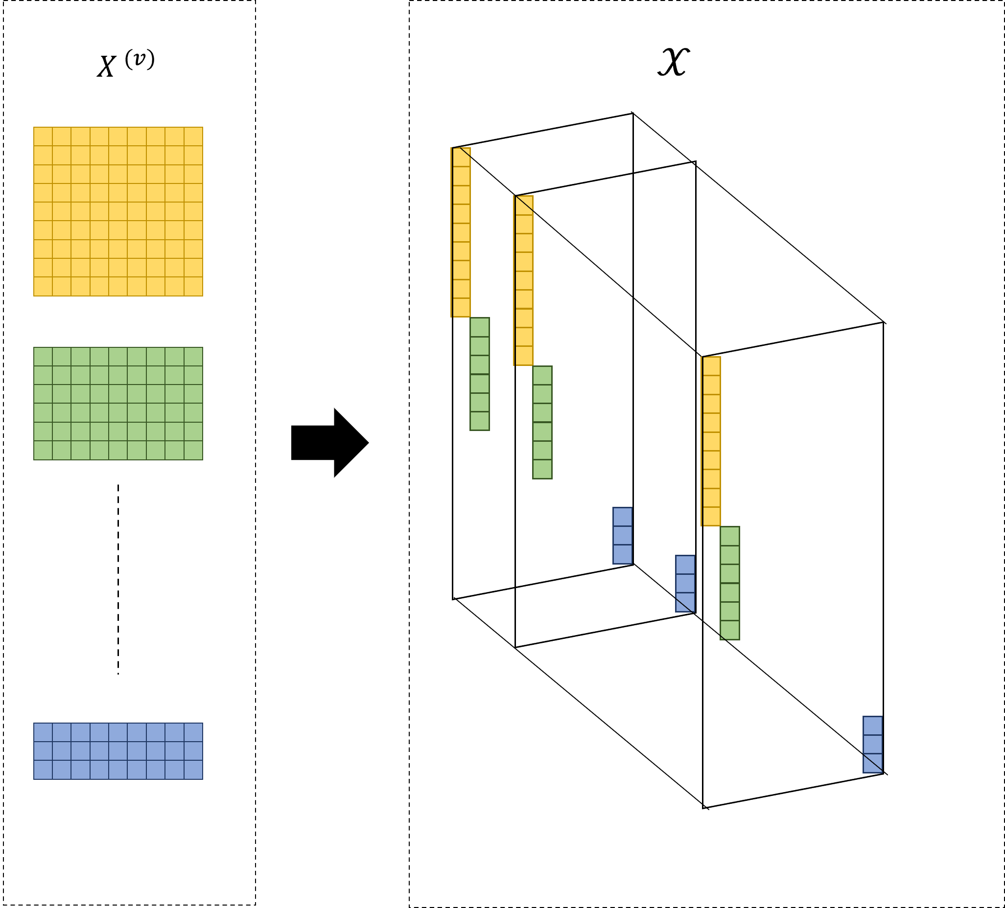
Figure 1: Constructing a third order tensor from the matrices in $\mathbb{R}^{d_{v}\times n}$

By following these steps, we can rid of the variable dimension, while preserving the structure of tha data.

4.1 Multi-view graph clustering

Multi-view graph clustering aims to find a fusion graph of all views, then apply the classical clustering methods on the fusion graph, as spectral clustering or graph-cut algorithms to produces the final clustering.

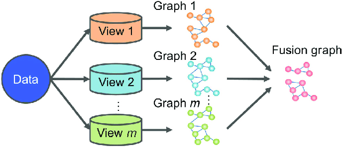
Figure 2: The general method of multi-view graph-based clustering Yang and Wang (2018)

Spectral clustering relies on computing the eigenvectors of the graph Laplacian matrix.
One of the most representative spectral clustering methods is the co-regularized spectral clustering. It performs standard spectral clustering on each view to get the corresponding indicator matrix, and then gets the common indicator matrix by minimizing disagreement between indicator matrices. However, it treats each indicator matrix equally, which is not ideal in real applications.

As it is said, the challenge is how to assign an appropriate weight to each view, even though we find some method Chaudhuri et al. (2009) that don’t bother themselves of these different views, this strategy neglects the importance of different graphs and may suffer when an unreliable graph is added to, other methods like in Xia et al. (2010) adds new hyper parameters, but it’s effect on the clustering is cannot be underestimated, and other methods try, to learns the weight automatically, which eliminates the need of any additional hyper parameter, as we present some.

The method used in Auto-weighted Multiple Graph Learning (AMGL) Nie et al. (2016), supposes that the normalized Laplacian matrices $L_{S}^{(v)}$ are constructed, and then solve the following problem:

$$\min_{F\in\mathbb{R}^{n\times c}F^{T}F=\mathbf{I}}\sum_{v=1}^{V}\sqrt{\operatorname{Tr}\left(F^{T}L_{S}^{(v)}F\right)}.$$ (11)

which is solved by fixing the parameters $\alpha$ then solves:

$$\min_{F\in\mathbb{R}^{n\times c}F^{T}F=\mathbf{I}}\sum_{v=1}^{V}\alpha^{(v)}\operatorname{Tr}\left(F^{T}L_{S}^{(v)}F\right).$$

Then, the parameters is updated using the formula:

$$\alpha^{(v)}=\dfrac{1}{\operatorname{Tr}\left(F^{T}L_{S}^{(v)}F\right)}.$$

The method can also be used for semi supervised clustering, but it is not in the scope of this review. In AMGL method, there are no hyper parameters, it can learns both the weight of each view and also the embedding matrix $F$, and then we treat each row of $F$ as a new representation of each data point and compute the clustering labels by using k-means algorithm.

After merging the view, some methods modify the traditional spectral clustering framework, they don’t need to search the uniform similarity matrix, but instead, try to learn an indicator matrix, that is used directly for clustering. One can also impose a constraint Laplacian rank, which guarantees that we have c clusters (components in the language of graphs), as stated by the following theorem.

Theorem 1

(Marsden, 2013) The multiplicity c of the eigenvalue 0 of the Laplacian matrix $L_{S}$ is equal to the number of connected components in the graph with the similarity matrix $S$.

In (Nie et al., 2017a), a Parameter-weighted Multi view Clustering (PwMC) method has been proposed. This method is based on the generalization of the CLR method: It learns a new similarity matrix from the old similarities of the v-th view $S^{(v)}$, computed from the original data:

$$\min_{w_{(v)},U} \sum_{v=1}^{V}w^{(v)}\left\|U-S^{(v)}\right\|_{F}^{2}+\gamma\|w\|_{2}^{2}$$ (12)

s.t. $$w_{(v)}\geq 0,\mathbf{1}_{v}^{T}\mathbf{w}=1,u_{ij}\geq 0,\mathbf{1}^{T}\mathbf{u}=1$$

$$\operatorname{rank}\left(L_{U}\right)=n-c.$$

The rank constraint is hard to tackle, since the diagonal matrix $D_{S}$ depends also on $S$. As the Laplacian is positive semi-definite, it’s eigenvalues are positive, which makes the constraint rank: $\operatorname{rank}\left(L_{U}\right)=n-c$ can be ensured by $\sum_{i=1}^{c}\sigma_{i}\left(L_{U}\right)=0$, where $\sigma_{i}(V)$ represents the i-th smallest eigenvalue of a matrix $M$. Thus we can replace the constraint, by adding $\lambda\sum_{i=1}^{c}\sigma_{i}\left(L_{U}\right)$ to the objective function, with $\lambda$ large enough. In addition, we can further make the objective function easier to solve, since we have the following theorem:

Theorem 2

(Fan et al., 1949) We have the following result

$$\sum_{i=1}^{c}\sigma_{i}\left(L_{S}\right)=\min_{F\in\mathbb{R}^{n\times c},F^{T}F=\mathbf{I}}\operatorname{Tr}\left(F^{T}L_{S}F\right).$$

The method depends on the hyper parameter $\gamma$, which affects the clustering accuracy since it is confirmed to be dataset-related. A new method proposed named Self-weighted Multi-view Clustering (SwMC) (Nie et al., 2017b), deals with this problem by removing completely $\gamma\|w\|_{2}^{2}$, from the equation (12).

As SwMc, supposes that the similarity matrix of each view is given, or calculated separately by k-means for example, Some approaches bypass this stage since the performance is significantly dependent on the view graphs that are generated. Due to the complex distribution of data in real-world applications, it is challenging to manually create a suitable similarity graph. When the graph quality is inadequate, the performance of these approaches drops dramatically. This decreases the algorithm flexibility. One solution is to calculate the similarity matrix directly from the data points, which is found more reliable and noise reducing, in addition, it calculates the weights automatically and eliminates the post processing step as well, the method named Multi-View Clustering and Semi-Supervised Classification with Adaptive Neighbours (MLAN) (Nie et al., 2017a) solves the following problem:

$$\min_{S}\sum_{v=1}^{V}\sqrt{\operatorname{tr}\left(X^{(v)}L_{S}X^{(v)}\right)}+\alpha\|S\|_{F}^{2}$$ (13)

$$\text{ s.t. }\mathbf{s}_{i}^{T}\mathbf{1}=1,0\leq s_{ij}\leq 1,\quad\operatorname{rank}\left(L_{S}\right)=n-c,$$

Where the following relationship is used instead in (Nie et al., 2017a) :

$$\sum_{v=1}^{V}\operatorname{tr}\left(X^{(v)}L_{S}X^{(v)}\right)=\sum_{v=1}^{V}\sum_{i,j}\left\|\mathbf{x}_{i}^{(v)}-\mathbf{x}_{j}^{(v)}\right\|_{2}^{2}s_{ij}.$$ (14)

This part (14) is usually added to give an affinity matrix the following property: High intra-cluster similarity and low inter-cluster similarity: For each data point $x_{i}$, it belongs to one of the c classes, and can be connected by any other data point $x_{j}$ with a probability $s_{ij}$, this probability can be seen as the similarity between the points, thus, a large probability should be given to the closer sampler, in other words, a small distance $\left\|\mathbf{x}_{i}^{(v)}-\mathbf{x}_{j}^{(v)}\right\|_{2}^{2}$, which justifies the first part of the equation. In other words, the multi-view graph embedding tries to preserve the local structure of the graphs, and graphs with similar local structure tend to be close to each other in the original multi-view feature space.
MLAN only learns a global graph for all views (without building a graph for each view), thus a method named Graph-based Multi-view Clustering (GMC) Wang et al. (2020) tries to find both while guarding the same objective:

$$\min_{S^{(v)},U} \sum_{v=1}^{V}\left(\operatorname{tr}\left(X^{(v)}L_{S}X^{(v)}\right)+\beta\left\|S^{(v)}\right\|_{2,1}^{2}\right)$$ (15)

$$+\sum_{v=1}^{V}w_{v}\left\|U-S^{(v)}\right\|_{F}^{2}+2\lambda\operatorname{Tr}\left(F^{T}L_{U}F\right)$$

$$\text{ s.t. }s_{ii}^{(v)}=0,s_{ij}^{(v)}\geq 0,\mathbf{1}^{T}\mathbf{s}_{i}^{(v)}=1,$$

$$u_{ij}\geq 0,\mathbf{1}^{T}\mathbf{u}_{i}=1,F^{T}F=\mathbf{I}.$$

As most methods used only one similarity graph. A recent work, (Rong et al., 2021) created a multi-metric similarity graph refinement and fusion strategy for MVC in which several similarity graphs were built using different metrics and an informative unified graph was obtained by adaptively fusing these similarity graphs.

4.2 Multi-view subspace clustering

Multi-view subspace clustering attempts to discover a latent space from all the different views in order to deal with high-dimensional data, and then applies a traditional clustering approach to this subspace.

Figure 3: The general method of multi-view subspace clustering Yang and Wang (2018)

It normally consists of the following steps:

1. Learning the latent matrices or tensors using various learning methods.

2. Computing the affinity (similarity) matrix by averaging latent matrices or tensors.

3. Applying spectral clustering on the similarity matrix.

Existing multi-view clustering algorithms may be divided into two types: Matrix-based and tensor-based representation learning.
Matrix theory, which organizes data in matrix form, is central to matrix-oriented approaches. It is discovered that this stream has a common flaw. It solves the problem by simply merging the views without taking into consideration the high-order correlations between these views at the same time, which is why the second stream (tensor-based representation), which has already received a lot of attention, will be the subject of this discussion. We can generalize certain single-view methods to multi-view ways by addressing the following problem:

$$\min_{Z^{(v)},E^{(v)}} \sum_{v=1}^{V}\left(\Psi(Z^{(v)})+\lambda\varphi(E^{(v)})\right)$$ (16)

s.t $$X^{(v)}=X^{(v)}Z^{(v)}+E^{(v)}.$$

After obtaining these multiple learned subspace representation $\left\{Z^{(v)}\right\}_{v=1}^{V}$, the final affinity matrix is calculated by combining all subspace representation of each view:

$$S=\dfrac{1}{2V}\sum_{v=1}^{V}\left(\mid{Z}^{(v)}\mid+\mid{Z}^{(v)^{\mathrm{T}}}\mid\right).$$ (17)

Finally, using the combined affinity matrix $S$, a spectral clustering approach or k-means is performed; however, this formulation ignores the link between subspaces and treats each subspace representation individually.

We get multiple subspace clustering methods by using alternative norms for the loss function and regularization term, to mention a few.

In the method named consistency-specificity multi-view subspace clustering (CSMSC) by Luo et al. (2018), they divided the learned subspace representation $Z^{(v)}$ into a learned consistent $C$ that is shared across the views, and specific self-representation matrices $D^{(v)}$ with data under different views, as for the regularization function, the nuclear norm is chosen for $C$, to guarantee the low rank property in order to excavate more shared information among different views, and the $l_{2}$ norm for $D^{(v)}$ for the connectedness property, and the $l_{21}$ norm for the loss function:

$$\min_{C,D^{(v)},E^{(v)}} \lambda_{1}\|C\|_{*}+\lambda_{2}\sum_{v=1}^{V}\left(\left\|D^{(v)}\right\|_{2}^{2}+\left\|E^{(v)}\right\|_{2,1}\right)$$ (18)

s.t. $$X^{(v)}=X^{(v)}\left(C+D^{(v)}\right)+E^{(v)}.$$

In this case, the learned affinity matrix is calculated differently:

$$S=\frac{\mid C\mid+\mid C^{T}}{2}\mid+\frac{1}{2V}\sum_{v=1}^{V}\mid D^{(v)}\mid+\mid D^{(v)}\mid^{T}.$$ (19)

Instead of the classical independence tests such as Spearmans rho and Kendalls tau that can only discover linear relationships. In the paper diversity-induced Multi-view Subspace Clustering (DiMSC), Cao et al. (2015) used The Hilbert Schmidt Independence Criterion (HSIC) (the empirical version) as a diversity term in to recover the links between distinct subspace representations, and to enhance the complementary between the multi-view representations.

4.3 Tensorized MVC

4.3.1 Tensorized subspace based MVC

As previously stated, treating data as matrices rather than as a full tensor implies that the relationship between subspace is neglected, and the tensor-based problem often solves the following problem:

$$\min_{\mathcal{Z},\mathcal{E}} \psi(\mathcal{Z})+\lambda\varphi(\mathcal{E})$$ (20)

S.t. $$X^{(v)}=X^{(v)}Z^{(v)}+E^{(v)}$$

$$\mathcal{Z}=\Phi_{1}\left(Z^{(1)},Z^{(2)},\ldots,Z^{(V)}\right)$$

$$\mathcal{E}=\Phi_{2}\left(E^{(1)},E^{(2)},\ldots,E^{()}\right),$$

where $\Phi$ is a suitable regularized tensor norm, $\varphi$ is a valid tensor norm for noise cancellation or sparsity, and the functions $\Phi_{1}$ and $\Phi_{2}$ produce the tensor $\mathcal{Z}$ and $\mathcal{E}$ by merging various matrices $Z(v)$ and $E(v)$ respectively, to a three-mode tensor. It was intended to define two functions rather than one since various techniques may utilize them differently; hence, $\Phi_{1}$ rotates the tensor as shown in the figure 4.

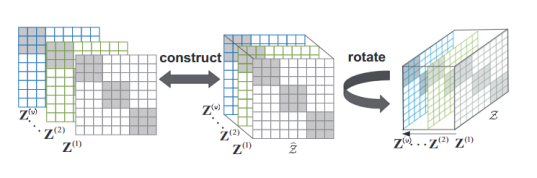
Figure 4: Tensor construction and rotation it

Tensor rotation can be advantageous in a variety of ways: Because it performs the transformation along the third dimension, the coefficients of the representation matrices are kept in the Fourier domain, reducing computing complexity greatly.

For example, inspired by the essential connection between spectral clustering and the Markov chain, a method called essential tensor learning for multi-view spectral clustering (TLMSC) Wu et al. (2018) builds a tensor based on multi-view transition probability matrices of the Markov chain; It first creates a similarity matrix of each view, then generates the transition probability $P^{(v)}=D^{(v)^{-1}}S^{(v)}$, and feeds it to the proposed model:

$$\min_{\mathcal{Z},\mathcal{E}}\|\mathcal{Z}\|_{\circledast}+\lambda\|\mathcal{E}\|_{2,1}$$ (21)

$$\text{ s.t. }\mathcal{P}=\mathcal{Z}+\mathcal{E}$$

$$\mathcal{P}=\Phi_{1}\left(P^{(1)},P^{(2)},\ldots,P^{(V)}\right),$$

where $\phi_{1}$ constructs and rotates the tensor to $n\times V\times n$.
TLMSC gives impressive result, however it employs the soft thresholding function to shrink each singular values with the same parameter. As a result, the prior knowledge of matrix singular values is not used even if it is important for the clustering, thus a method known as weighted tensor-nuclear norm minimization (WTNNM) Xie et al. (2021) is introduced to deal with this issue; It shrinks singular values with different parameters and captures the high order correlation underlying multi-view data by using $\psi$ as the weighted nuclear norm of tensor rather than the tensor nuclear norm.
The present tensor-nuclear norm minimization keeps some big singular values while rejecting others. This suggests that the bigger single values are significant, whilst the lower singular values are insignificant. However, in practice, such an assumption is not always correct, and higher single values may include unwanted information.
In Cheng et al. (2019), a method named tensor based Representation Learning method for Multi-view Clustering (tRLMvC) Cheng et al. (2019), adopts a different idea than the previous ones presented, it searches the representation tensor using T- product, then performs a factorization via the Tucker decomposition, the problem that is solved is:

$$\min_{\mathcal{Z},\mathcal{C},U_{1},U_{3},U_{3}} \|\mathcal{X}-\mathcal{X}*\mathcal{Z}\|_{F}^{2}+\alpha\|\mathcal{Z}\|_{FF1}$$ (22)

$$+\beta\left\|\mathcal{Z}-\mathcal{C}\times_{1}U_{1}\times_{2}U_{2}\times_{3}U_{3}\right\|_{F}^{2},$$

Then, any single view clustering algorithm such as k-means may be employed on the matrix $H=[U_{1},U_{2}]$, with the column vector $U_{3}$ characterizing the contribution of each view.

4.3.2 Tensorized graph based MVC

To acquire clustering results, current matrix-based algorithms execute traditional spectral clustering after collecting the similarity matrix. None of them explore how to increase the stability of spectral clustering or how to utilize higher order correlation in data, hence the tensor-based technique is introduced to address this issue.

To obtain the clustering results, the approach in Xie et al. (2018) first pursues the subspace representation tensor using the tensor nuclear norm (different tensor rank approximations used in similar methods) before generating the final affinity matrix. Of this way, the two primary components of spectral clustering; The representation tensor and the affinity matrix, are learnt separately.

To address this issue, a method named Graph regularized Low-rank Tensor representation and the Affinity matrix (GLTA) Chen et al. (2019) solves the problem by simultaneously learning the representation tensor and the affinity matrix, with the following optimization problem:

$$\min_{\mathcal{Z},\mathcal{E},S,\omega} \sum_{v=1}^{V}\Big{(}\alpha\operatorname{tr}\left(Z^{(v)}L^{(v)}Z^{(v)^{T}}\right)+\beta\omega_{v}\left\|Z^{(v)}-S\right\|_{F}^{2}\Big{)}+\|\mathcal{E}\|_{2,1}$$ (23)

$$\text{ s.t. }X^{(v)}=X^{(v)}Z^{(v)}+E^{(v)}$$

$$\mathcal{Z}=\mathcal{C}\times{}_{1}U_{1}\times{}_{2}U_{2}\times{}_{3}U_{3},U_{i}^{\prime}U_{i}=I$$

$$\mathcal{E}=\Phi_{2}\left(E^{(1)},E^{(2)},\ldots,E^{(V)}\right),\quad\omega_{v}\geq 0,\mathbf{1}^{T}\mathbf{\omega}=1,$$

where $L^{(v)}$ is the normalized Laplacian matrix, GLTA learns also the local view-specific geometrical structures and the diverse contributions of distinct attributes. Specifically, when creating the final affinity matrix, it uses the Tucker decomposition to encapsulate the low-rank attribute, the manifold regularization to show the local view-specific geometrical structures, and gives appropriately varying weights to distinct characteristics.

In the method Task-driving affinity matrix for accurate Multi-view clustering (TAMMC), Wang et al. (2021) tries to preserve the local affinities of all views via a graph regularization on self-expressive tensor, by penalizing a Laplacian rank on a learned common subspace by solving the following problem:

$$\min_{S,\mathcal{Z}} \sum_{v=1}^{V}\left(\alpha\operatorname{Tr}\left(Z^{(v)}L^{(v)}Z^{(v)^{T}}\right)+\lambda\|S-Z^{(v)}\|_{F}^{2}\right)$$ (24)

$$+\frac{1}{2}\|\mathcal{X}-\mathcal{X}*\mathcal{Z}\|_{F}^{2}+\theta\|\mathcal{Z}\|_{TNN}$$

$$\text{ s.t. }\quad\mathbf{1}^{T}\mathbf{s}_{i}=1,\quad s_{ij}\geqslant 0,\operatorname{rank}\left(L_{S}\right)=n-c,$$

where, the Laplacian matrix of each view, is calculated using Gaussian distance based on t-nearest neighbors. The first term represents the approximation error using the Tensor Frobenius norm, the second and third terms penalize the tensor representation, thereby making it low-rank and imposing the estimated subspace to preserve the local affinity (Samples that are near in raw space are likely to remain close in the mapped subspace). The last term is used to make a consensus representation. With the rank Laplacian constraint condition, the affinity matrix is used directly for clustering.

A more recent work, a method named Multi-view Spectral Clustering with Adaptive Graph Learning and Tensor Schatten p-norm Zhao et al. (2022), which the suggested problem is:

$$\min_{F,\mathcal{Z},\mathbf{w},\mathbf{\alpha}} \sum_{v=1}^{V}\left(\frac{1}{w_{v}}\operatorname{tr}\left(X^{(v)}L^{(v)}X^{(v)}\right)+\lambda\frac{1}{\alpha_{v}}\operatorname{Tr}\left(F^{T}L^{(v)}F\right)\right)+\beta\|\mathcal{Z}\|_{Sp}^{p}$$ (25)

s.t. $$F^{T}F=\mathbf{I},\mathbf{1}^{T}\mathbf{z_{i}^{(v)}}=1,z_{ij}^{(v)}\geqslant 0$$

$$\mathbf{1}^{T}\mathbf{w}=1,w_{v}\geqslant 0,\mathbf{1}^{T}\mathbf{\alpha}=1,\alpha_{v}\geqslant 0,$$

where $L^{(v)}$ is the Laplacian matrix of the corresponding similarity matrix $Z_{(v)}$. The Schatten p-norm regularizer is used to minimize the divergence between graphs. It guarantees also that the rank of the learned graph approximates the target rank, i.e. cluster number.
In practice, noises and redundancy information are frequently mixed in with the original features. As a result, the consensus similarity graph that was learned m may be erroneous. Li et al. (2022) overcomes this issue by training the adaptive neighbor graph in a new low dimensional embedding space rather than the original feature space. First, it employs the view-specific similarity graph $W^{(v)}$ using an adaptive neighbor graph learning:

$$\forall i=1,...,n \min_{W^{(v)}_{i}}\sum_{j=1}^{n}\left\|x_{i}^{(v)}-x_{j}^{(v)}\right\|_{2}^{2}w^{(v)}_{ij}+\gamma w_{ij}$$ (26)

$$w^{(v)}_{ij}\geq 0,\mathbf{1}^{T}\mathbf{w}^{(v)}_{i}=1.$$

The new low-embedding space is learnt:

$$\min_{F^{(v)},\mathcal{T}} -\lambda\sum_{v=1}^{V}\operatorname{tr}\left(F^{(v)}A^{(v)}F^{(v)^{T}}\right)+\frac{1}{2}\|\mathcal{F}-\mathcal{T}\|_{F}^{2}+\|\mathcal{T}\|_{w,*}$$ (27)

$$\text{ s.t. }F^{(v)^{T}}F^{(v)}=\mathbf{I}_{c}$$

$$\mathcal{F}=[\overline{F}^{(1)}\overline{F}^{(1)^{T}};\cdots;\overline{F}^{(n)}\overline{F}^{(n)^{T}}],$$

where the normalized spectral embedding matrix $\overline{F}^{(v)}$ is obtained by normalizing the rows of $F^{(v)}$, and the normalized affinity matrix is

$$A^{(v)}=D^{(v)^{-0.5}}W^{(v)}D^{(v)^{0.5}},$$ (28)

and the tensors $\mathcal{F},\mathcal{T}\in\mathbf{R}^{n\times V\times n}$. Lastrly, the consensus graph $S$ can be learned using:

$$\min_{S} \sum_{v=1}^{V}\sum_{i,j=1}^{n}\left\|\overline{f}_{i}^{(v)}-\overline{f}_{j}^{(v)}\right\|_{2}^{2}s_{ij}+\gamma s_{ij}$$ (29)

$$s_{ij}\geq 0,\mathbf{1}^{T}\mathbf{s}_{i}=1.$$

5 Experiments

In this section, we do some experiments on various data sets, with varying amounts of samples, views, and clusters. This allows for a thorough evaluation of the performance of the various algorithms.
For the algorithms that has $\lambda\sum_{i=1}^{c}\sigma_{i}(L)$ minimization part. We set $\lambda=1$, as most of the papers in their codes, in each iteration, we double $\lambda$ if the number of components is less than the number of clusters wanted, and we divide it by 2, if the number of components is less than c. In practice, we can know the comparison between the number of components and the number of clusters mentioned in Marsden (2013) using the fact that if $\sum_{i=1}^{c+1}\sigma_{i}(L)\leq 0$ implies to the fact that number of connected components of the graph is larger than c, and $\sum_{i=1}^{c}\sigma_{i}(L)\geq 0$ implies that number of connected components of the graph is smaller than c.

5.1 Data sets

We used multiple different real world data sets used, that are commonly used in the literature, Which can be categorized into 3 Types: document, image and graph. The majority of image multi-view data sets are derived from initial single-view image data sets. The popular pre-computed multi-view picture data sets are shown. Readers can also create such multi-view data sets on their own for future research.
The vast majority of image multi-view data sets are created from single-view image data sets. Popular pre-computed multi-view image data sets are displayed. The document data sets are either obtained from a single view data set or naturally described in numerous views. Readers can also generate their own multi-view data sets for future investigation.

• One-hundred plant species leaves data set leafs (100Leaves) : It consists of 1600 samples, of 100 different species, 4 views are given: shape descriptor, fine scale margin and texture histogram.

• Handwritten digit data set. : is from the UCI repository. It consists of 2000 samples of handwrittend digits, with a 6 views, It has 10 clusters (0-9).

• 3 sources data set (3Sources) : It consists of 169 news, provided by three news companies, including the BBC, Reuters, and The Guardian. Each piece of news was manually labeled with one of six relevant designations.

• WebKB data set (WebKB) : It consists of 203 web pages, gathered from computer science departments of university, with 4 classes, each single web page is described by the title, the content of the page and the anchor text of the hyperlink.

• BBC data set(BBC) : It consists of 685 documents collected from the BBC news website. Each document has 4 segments with 5 manually annotated labels.

While these are provided as raw features, some graph-based approaches employ the similarity matrix as the input of each view, giving the user several options for how to generate the graph( as complete or k-nn…) and the metrics( as binary,cosine, or gaussian kernel…) from the raw input features. We generate exhaustive graphs from the same data set as previously, and we display the best performance on the best graph. We also included two pre-computed graph data sets:

• MSRC-v1 is a class-based picture collection from Microsoft Research in Cambridge containing 240 samples, with 7 classes. Each picture is represented by 6 distinct features: the HOG, the Color moment, the CENT, the LBP, the CENTRIST, and the SIFT feature.

• Yale Face Database(Yale) The database contains 165 GIF images with 15 classes. There are 11 ²s per subject.

• 17 Category Flower Dataset(Flo17) is a class-based picture of 17 type of flowers, with 80 images of each class, which means, a total of 1360 samples. It has 17 distinct features.

The characteristics of these raw feature data sets are given in the table below 2, which displays the number of samples, views, clusters, and $d_{v}$, which represents the dimension of features in view $v$. More information on the data set may be obtained by following the hyperlinks in the footnotes.

Table 2: Summary of the benchmark data sets used

Data set	# samples	# views	# clusters	$\mathrm{d}_{1}$	$d_{2}$	$d_{3}$	$d_{4}$	$d_{5}$	$d_{6}$
3Sources	169	3	6	3560	3631	3068	-	-	-
WebKB	203	3	4	1703	230	230	-	-	-
100Leaves	1600	3	100	64	64	64	-	-	-
BBC	685	4	5	4659	4633	4665	4684	-	-
HW	2000	6	10	216	76	64	6	240	47

5.2 Compared methods

Following that, we will compare the state of the art algorithms, for which public code, A couple modification were done on these data set in order to work with the same data set, and to work with the same clustering measures. The k-means algorithm adopted is also available. Note that the code of some algorithms were created from scratch, since they were not available to the public, but we majorly focused on the methods that the code exist in any programming language. The different methods are summarized in the table below, where we’ve devised the methods on two columns: Methods using the matrix related theory, the ones used the tensor related theory. We distinguish by emphasizing the methods that require the similarity matrices instead as input.

Table 3: Benchmark methods

Matricized		Tensorial
GBS	CSMSC	t-SVD-MSC
GMC	MVLRSCC	MVSC-TPR
MCGC	MVGL	CGL
AMGL	MLAN	MVSC-TLRR
SwMC	RG-MVC	MCSCS p_norm

5.3 Evaluation metrics

Each algorithm is run ten times to randomize the experiments. Different measures are utilized to evaluate the performance of these multi view clustering algorithms based using well-known benchmark data sets. In the clustering task, several measures favor various traits.
The accuracy (ACC), the normalized mutual information (NMI), the F1 measure (F-measure), and the adjusted rand index (ARI) are the main ones used:

- NMI (Strehl and Ghosh, 2002) is an information theoretic metric that measures the mutual information between the cluster assignments and the ground truth labels. It is normalized by the average of entropy of both ground labels and the cluster assignments, it even allows the comparison of two partitions even with a different number of clusters:

$$NMI=\dfrac{2I(\Omega,\Theta)}{H(\Omega)H(\Theta)},$$ (30)

where $I$ represents the mutual information, and $H$ the information entropy.
$\Omega=\{\omega_{1},\omega_{2},\ldots,\omega_{K}\}$ is the set of clusters and $\Theta=\{c_{1},c_{2},\ldots,c_{J}\}$ is the set of classes.
-ARI (Hubert and Arabie, 1985) computes a similarity measure between two clustering by considering all pairs of samples and counting pairs that are assigned in the same or different clusters in the predicted and true clustering. The adjusted Rand index is the corrected-for-chance version of the Rand index. It also allows the comparison of two partitions with different number of clusters:

$$ARI =\dfrac{RI-Expected(RI)}{max(RI)-Expected(RI)}$$ (31)

$$=\dfrac{\sum_{ij}{\binom{n_{ij}}{2}}-\frac{1}{\binom{n}{2}}\sum_{i}{\binom{n_{i}}{2}}\sum_{j}{\binom{n_{j}}{2}}}{{\frac{1}{2}}\left[\sum_{i}{\binom{n_{i}}{2}}+\sum_{j}{\binom{n_{j}}{2}}\right]-\frac{1}{\binom{n}{2}}\sum_{i}{\binom{n_{i}}{2}}\sum_{j}{\binom{n_{j}}{2}}},$$

where $n$ represents the number of samples, $n_{i}=\#c_{i}$ is the number of samples in the cluster $c_{i}$, while $n_{j}=\#w_{j}$ is the number of samples in the class $w_{j}$ and $n_{i}^{j}=\#\lvert w_{i}\cap c_{j}\rvert$ is the number of data points of cluster $w_{i}$ assigned to the class $c_{j}$.
In general, an ARI value lies between 0 and 1. The index value is equal to 1 only if a partition is completely identical to the intrinsic structure and close to 0 for a random partition.
-Purity(Manning et al., 2008) is a simple and transparent evaluation of the degree of each cluster containing a class of data points. It’s value can be calculated via the following formula:

$$Purity=\frac{1}{n}\sum_{i}\max_{j}n_{i}^{j}.$$ (32)

-ACC (Lovasz and Plummer, 1986) is the unsupervised counterpart of classification accuracy. It differs from usual accuracy metrics in that it employs a mapping function $map$ to determine the optimal mapping between the algorithm’s cluster assignment output $Y$ and the ground truth $Y^{0}$. This mapping is essential because an unsupervised algorithm may use a label other than the actual ground truth label to describe the same cluster, The best mapping can be found by using the Kuhn–Munkres algorithm in Lovasz and Plummer (1986):

$$ACC=\max_{map}\dfrac{\sum_{i=1}^{n}\delta(Y_{i}^{0},map(Y_{i}))}{n},$$ (33)

where $\delta(a,b)$ is a judgment function, it gives 1 if $a=b$ and 0 otherwise.
-$F_{\beta}$ measure is another metric that will be used, that can be calculated from the recall $R$ and the precision $P$ of a test, there is another parameter $\beta$( where it will be used equals to 1 in the numerical tests), which gives us the control of penalizing the false negatives more strongly than false positives by selecting a value greater than 1, as in ACC, we also used the permutation mapping that maximizes the matching of ground truth and predictive labels:

$$P=\frac{TP}{TP+FP}\qquad R=\frac{TP}{TP+FN}\qquad F_{\beta}=\frac{(\beta^{2}+1)PR}{\beta^{2}P+R},$$

where $TP,TN,FP$, and $FN$ denote the number of similar pairs (same class) assigned to the correct cluster, number of dissimilar pairs (different class) assigned to the wrong correct cluster, number of dissimilar pairs assigned to the wrong cluster, and number of similar pairs assigned to the wrong cluster, respectively.
For all metrics, a higher value indicates the better performance of the clustering.

5.4 Comparison result and analysis

For some methods, a post clustering (k -means) is needed on the obtaining embedding data, as it is sensitive to initial values, we repeat the k-means clustering processing 20 trials to avoid the randomness perturbation and report the result with the lowest value for the objective function of k-means clustering among the 20 results.
The comparison results are shown in Tables 8, 7, 5, 4, and 6. The best value of each measure is shown in bold. We note that the standard deviation is avoided to be show for the k-means clustering trials since simply, not all the methods use it, we also mention that the values are rounded to the ten-thousandths:

Table 4: Clustering measure on 3sources data set

Method	Fscore	Precision	Recall	NMI	ARI	ACC	Purity
CGL	0.6224	0.7097	0.5555	0.6800	0.5263	0.6604	0.7976
GBS	0.7159	0.6052	0.8760	0.7096	0.6082	0.7692	0.8047
GMC	0.6047	0.4844	0.8045	0.6216	0.4431	0.6923	0.7456
AMGL	0.2765	0.1711	0.7604	0.8490	0.2652	0.6352	0.7028
T-SVD-MS	0.7029	0.7100	0.6961	0.6362	0.6098	0.7547	0.7967
MVSC-TPR	0.5420	0.5722	0.5172	0.4561	0.4117	0.5979	0.6757
CSMSC	0.3800	1.0000	0.2346	0	0	0.3299	1.0000
MVGL	0.3455	0.2255	0.7381	0.1522	0.0163	0.3846	0.4320
Pairwise MLRSSC	0.6443	0.6045	0.6969	0.6167	0.5460	0.6840	0.7491
Centroid MLRSSC	0.5662	0.4629	0.7492	0.6470	0.4725	0.6482	0.6683
PairwiseKMLRSSC	0.4675	0.3798	0.6118	0.4837	0.3525	0.5098	0.5240
Centroid KMLRSSC	0.4745	0.3847	0.6214	0.4824	0.3620	0.5169	0.5272
MLAN	0.9112	0.9112	0.9112	0.7881	0.8171	0.9112	0.9112

Table 5: Clustering measure on WebKB data set

Method	Fscore	Precision	Recall	NMI	ARI	ACC	Purity
CGL	0,5025	0,6249	0,4202	0,3178	0,2725	0,4729	0,7783
GBS	0,7227	0,6148	0,8766	0,465	0,4844	0,7833	0,798
GMC	0,6878	0,5821	0,8404	0,4133	0,4169	0,7586	0,7734
AMGL	0,5489	0,3925	0,9128	0,037	-0,002	0,5099	0,5308
T-SVD-MS	0,562	0,5642	0,5609	0,2536	0,2772	0,6182	0,6805
MVSC-TPR	0,4751	0,5664	0,4092	0,2042	0,217	0,5539	0,6941
CSMSC	0,4533	0,2435	0,509	0,4755	0,2983	0,4102	0,4835
MVGL	0,6144	0,5761	0,6581	0,2805	0,3358	0,6995	0,7389
Pairwise MLRSSC	0,4453	0,3339	0,6746	0,3675	0,2504	0,4204	0,4493
Centroid MLRSSC	0,3816	0,2629	0,7036	0,3539	0,214	0,3963	0,4032
Pairwise KMLRSSC	0,4655	0,3818	0,6021	0,2438	0,2338	0,5234	0,57
Centroid KMLRSSC	0.4528	0.3649	0.6043	0.237	0.2264	0.5015	0.5436
MLAN	0.3448	0.7881	0.2226	0.4921	0.5119	0.7881	0.8029

Table 6: Clustering measure on 100Leaves data set

Method	Fscore	Precision	Recall	NMI	ARI	ACC	Purity
CGL	0,6245	0,7097	0,5654	0,6871	0,5263	0,6604	0,8024
GBS	0,3867	0,2555	0,7951	0,8711	0,3779	0,6694	0,7131
GMC	0,5042	0,3521	0,8874	0,9292	0,4974	0,8237	0,8506
AMGL	0,2765	0,1711	0,7604	0,849	0,2652	0,6352	0,7028
T-SVD-MS	0,8549	0,9428	0,7825	0,9708	0,8534	0,8568	0.9606
MVSC-TPR	0,5787	0,5209	0,6515	0,8532	0,5743	0,6607	0,7028
CSMSC	0,3455	0,5543	0,4521	0.6433	0,3894	0,3467	0,4870
MVGL	0,2299	0,1545	0,4491	0,732	0,219	0,5056	0,5463
Pairwise MLRSSC	0,0186	0,9994	0,0094	0,0006	0	0,0103	0,9997
Centroid MLRSSC	0,0186	0,9991	0,0094	0,0009	0,000	0,0104	0,9995
Pairwise KMLRSSC	0,0824	0,6515	0,044	0,4501	0,066	0,0781	0,7601
Centroid KMLRSSC	0.4528	0.0821	0.663	0.0438	0.4523	0.0656	0.0784
MLAN	0.0706	0.0706	0.0706	0.9494	0.8242	0.87375	0.8956

Table 7: Clustering measure on BBC data set

Method	Fscore	Precision	Recall	NMI	ARI	ACC	Purity
CGL	0,9061	0,8906	0,9269	0,9185	0,8761	0,8886	0,9296
GBS	0,5451	0,4031	0,8414	0,4839	0,3337	0,6044	0,6102
GMC	0,6333	0,5012	0,86	0,5628	0,4789	0,6934	0,6934
AMGL	0,3748	0,238	0,8891	0,02	0,0082	0,3431	0,3477
T-SVD-MS	0,3516	0,7055	0,2361	0,0896	0,0034	0,3396	0,8132
MVSC-TPR	0,574	0,6430	0,4039	0,3498	0,2344	0,4366	0,8132
CSMSC	0,48374	0,5903	0,6345	0,243	0,245	0,245	0,674
MVGL	0,3686	0,2329	0,8841	0,0806	0,0043	0,3489	0,3509
Pairwise MLRSSC	0,7291	0,6643	0,8118	0,7213	0,6571	0,7302	0,7673
Centroid MLRSSC	0,6498	0,5202	0,8669	0,6971	0,5751	0,6562	0,6562
Pairwise KMLRSSC	0,408	0,3338	0,5274	0,4228	0,2761	0,4622	0,4725
Centroid KMLRSSC	0.4051	0.3442	0.4948	0.4093	0.263	0.4661	0.4885
MLAN	0.5591	0.5591	0.5591	0.7274	0.7460	0.8715	0.8715

Table 8: Clustering measure on HW data set

Method	Fscore	Precision	Recall	NMI	ARI	ACC	Purity
CGL	0,8584	0,7941	0,963	0,9354	0,8405	0,8617	0,8741
GBS	0,8327	0,7788	0,8945	0,8787	0,8128	0,847	0,8655
GMC	0,8653	0,826	0,9085	0,9041	0,8496	0,882	0,882
AMGL	0,4011	0,3081	0,5788	0,6162	0,3115	0,5536	0,5893
T-SVD-MS	0,9042	0,9729	0,8464	0,9602	0,8926	0,8936	0,983
MVSC-TPR	0,6745	0,6346	0,8045	0,8341	0,7563	0,7732	0,7422
CSMSC	0,4354	0,6349	0,7409	0,753	0,65	0,632	0,6244
MVGL	0,6367	0,557	0,7429	0,7231	0,59	0,6895	0,7245
Pairwise MLRSSC	0,6498	0,5202	0,8669	0,6971	0,5751	0,6562	0,6562
Centroid MLRSSC	0,7266	0,8678	0,625	0,8021	0,6907	0,7438	0,9244
Pairwise KMLRSSC	0,5399	0,6179	0,4794	0,5958	0,4818	0,6361	0,7412
Centroid KMLRSSC	0.5399	0.6179	0.4794	0.5958	0.4818	0.6361	0.7412
MLAN	0.1965	0.1965	0.1965	0.9374	0.9384	0.972	0.972

As it shows from the tables, there is clearly, an advantage of using the tonsorial theory, these type methods has a batter performances on all kind of measures on most of the data.

Table 9: Clustering measure of graph methods on different data set

Method	Data set	Fscore	Precision	Recall	NMI	ARI	ACC	Purity
SwMC	3sources	0.5888	0.4637	0.8063	0.6036	0.4166	0.6746	0.7278
RG-MVC	3sources	0.4956	0.456	0.7963	0.6354	0.345	0.5244	0.6833
MCSCS p_norm	3sources	0.2768	0.3422	0.2324	0	0	0.3314	0.3442
MVSC-TLRR	3sources	0.5197	0.7299	0.4138	0.4498	0.3167	0.5707	0.8272
SwMC	BBC	0.6167	0.4846	0.8476	0.5534	0.4536	0.6964	0.6964
RG-MVC	BBC	0.3453	0.3948	0.7340	0.345	0.354	0.5464	0.345
MCSCS p_norm	BBC	0.38	0.439	0.2346	0	0	0.3299	0.3847
MVSC-TLRR	BBC	0.564	0.4566	0.4353	0.6309	0.3453	0.5635	0.7353
SwMC	Flower	0.2804	0.181	0.6221	0.5566	0.1506	0.5391	0.53
RG-MVC	Flower	0.1621	0.1834	0.1453	0.2342	0.1931	0.3453	0.2431
MCSCS p_norm	Flower	0.1773	0.1917	0.1654	0.2886	0.1225	0.2709	0.319
MVSC-TLRR	Flower	0.2666	0.2726	0.2609	0.4108	0.2203	0.3781	0.4082
SwMC	HW	0.7668	0.6849	0.8711	0.862	0.7376	0.75	0.787
RG-MVC	HW	0.6734	0.435	0.6543	0.739	0.945	0.6453	0.6953
MCSCS p_norm	HW	0.5026	0.5733	0.4505	0.5886	0.44	0.5969	0.6924
MVSC-TLRR	HW	0.7745	0.6934	0.8313	0.876	0.735	0.654	0.6941
SwMC	Leaves	0.3644	0.2949	0.4766	0.7625	0.3569	0.5581	0.5844
RG-MVC	Leaves	0.2409	0.2584	0.4209	0.7433	0.3583	0.5143	0.5243
MCSCS p_norm	Leaves	0.4079	0.4743	0.3582	0.7605	0.4015	0.5502	0.6264
MVSC-TLRR	Leaves	0.2138	0.3646	0.1517	0.6735	0.2032	0.4077	0.5272
SwMC	MSRCV1	0.8412	0.8304	0.8522	0.853	0.8152	0.919	0.919
RG-MVC	MSRCV1	0.4946	0.5314	0.4632	0.6326	0.4611	0.5855	0.6778
MCSCS p_norm	MSRCV1	0.3856	0.3314	0.4612	0.5936	0.3947	0.4634	0.4563
MVSC-TLRR	MSRCV1	0.7368	0.7988	0.6889	0.7824	0.6896	0.785	0.8667
SwMC	WebKB	0.7004	0.5919	0.8576	0.4351	0.4397	0.7685	0.7833
RG-MVC	WebKB	0.6433	0.5948	0.7003	0.4112	0.534	0.493	0.7103
MCSCS p_norm	WebKB	0.4945	0.4347	0.5734	0	0	0.5271	0.593
MVSC-TLRR	WebKB	0.6944	0.5903	0.8344	0.4230	0.4093	0.6734	0.7304
SwMC	Yale	0.7734	0.6343	0.6301	0.6781	0.6433	0.823	0.8423
RG-MVC	Yale	0.6434	0.6121	0.5834	0.6453	0.5498	0.7	0.7994
MCSCS p_norm	Yale	0.5759	0.6012	0.5529	0.6207	0.5041	0.6852	0.7212
MVSC-TLRR	Yale	0.7519	0.8386	0.6875	0.8278	0.7209	0.7841	0.9084

5.5 Further work

We can also, compare the time complexity, but since the methods are not all in the same language (Matlab and Python), we decided not to stop in order to not falsify the reel comparison between the methods.
For the graph based methods, we can further investigate the hyper graph, which differs from the graph by letting the edges to be associated to more than two nodes, as we can calculate the Laplacian by an appropriate formula, and then continue the rest of the word as the normal graphs, as in Lu et al. (2020), named HLR-MSCLRT, where the following objective is the same as in (20), by simply replacing the Laplacian of a graph matrix of a view $L^{(v)}$ by its Hyper graph Laplacian $L_{h}^{(v)}$.

6 Conclusion

As it is shown, for clustering multi view is the way to go, as it brings with its multiple views, multiple data that can give more information, having also new methods, a part from the ones that can be generalized from the single view, without forgetting the new challenges of how to combine and use all the views, the tensor representation of the data, has a clear advantages of just considering data as matrices, by exploiting the higher order correlation in the data, which has been used, different norms and ranks, The coherence and complimentary nature of diverse views of view are therefore automatically taken into account. Two main categories were mainly discussed are the graph based, and the subspace based, we can even give the graph based method more credits, as it gives insight on the local view specific geometrical structures, and can also be combined in some methods that tries to find a low rank representation tensor with a Laplacian term, while also some method tries to learn the affinity matrices of each view and others only the global affinity matrix.

References

- Li et al. [2019] Yingming Li, Ming Yang, and Zhongfei Zhang. A survey of multi-view representation learning. IEEE Transactions on Knowledge and Data Engineering, 2019. doi:10.1109/tkde.2018.2872063.
- Yang and Wang [2018] Yan Yang and Hao Wang. Multi-view clustering: A survey. Big Data Mining and Analytics, 1:83–107, 6 2018. ISSN 20960654. doi:10.26599/BDMA.2018.9020003.
- Zhao et al. [2017] Jing Zhao, Xijiong Xie, Xin Xu, and Shiliang Sun. Multi-view learning overview: Recent progress and new challenges. Information Fusion, 38:43–54, 2017. ISSN 1566-2535. doi:https://doi.org/10.1016/j.inffus.2017.02.007. URL https://www.sciencedirect.com/science/article/pii/S1566253516302032.
- Cai et al. [2013] Xiao Cai, Feiping Nie, and Heng Huang. Multi-view k-means clustering on big data. IJCAI, 2013. doi:null.
- Guo et al. [2014] Dongyan Guo, Jian Zhang, Xinwang Liu, Ying Cui, and Chunxia Zhao. Multiple kernel learning based multi-view spectral clustering. Proceedings - International Conference on Pattern Recognition, pages 3774–3779, 12 2014. ISSN 10514651. doi:10.1109/ICPR.2014.648.
- Kilmer and Martin [2011] Misha E. Kilmer and Carla D. Martin. Factorization strategies for third-order tensors. Linear Algebra and its Applications, 435:641–658, 8 2011. ISSN 0024-3795. doi:10.1016/J.LAA.2010.09.020.
- Kilmer et al. [2013] Misha E. Kilmer, Karen Braman, Ning Hao, and Randy C. Hoover. Third-order tensors as operators on matrices: A theoretical and computational framework with applications in imaging. https://doi.org/10.1137/110837711, 34:148–172, 2 2013. ISSN 08954798. doi:10.1137/110837711. URL https://epubs.siam.org/doi/10.1137/110837711.
- Hao et al. [2013] Ning Hao, Misha E. Kilmer, Karen Braman, and Randy C. Hoover. Facial recognition using tensor-tensor decompositions. http://dx.doi.org/10.1137/110842570, 6:437–463, 2 2013. ISSN 19364954. doi:10.1137/110842570. URL https://epubs.siam.org/doi/10.1137/110842570.
- Zhang et al. [2014] Zemin Zhang, Gregory Ely, Shuchin Aeron, Ning Hao, and Misha Kilmer. Novel methods for multilinear data completion and de-noising based on tensor-svd. 2014.
- Wu et al. [2020] Jianlong Wu, Xingxu Xie, Liqiang Nie, Zhouchen Lin, and Hongbin Zha. Unified graph and low-rank tensor learning for multi-view clustering. 2020. URL https://zhouchenlin.github.io/Publications/2020-AAAI-UGLTL.pdf.
- Liu et al. [2010] Guangcan Liu, Zhouchen Lin, and Yong Yu. Robust subspace segmentation by low-rank representation. ICML, 2010. doi:null.
- Elhamifar and Vidal [2013] Ehsan Elhamifar and René Vidal. Sparse subspace clustering: Algorithm, theory, and applications. IEEE Transactions on Pattern Analysis and Machine Intelligence, 35(11):2765–2781, 2013. doi:10.1109/TPAMI.2013.57.
- Wang et al. [2013] Yu Xiang Wang, Huan Xu, and Chenlei Leng. Provable subspace clustering: When lrr meets ssc. Advances in Neural Information Processing Systems, 2013. ISSN 10495258. doi:10.1109/TIT.2019.2915593.
- Chaudhuri et al. [2009] K Chaudhuri, S M Kakade, K Livescu, and K Sridharan. Multi-view clustering via canonical correlation analysis. 2009. doi:10.1145/1553374.1553391. URL http://dx.doi.org/10.1145/1553374.1553391.
- Xia et al. [2010] Tian Xia, Dacheng Tao, Tao Mei, and Yongdong Zhang. Multiview spectral embedding. IEEE Transactions on Systems, Man, and Cybernetics, Part B: Cybernetics, 40:1438–1446, 12 2010. ISSN 10834419. doi:10.1109/TSMCB.2009.2039566.
- Nie et al. [2016] Feiping Nie, Jing Li, and Xuelong Li. Parameter-free auto-weighted multiple graph learning: A framework for multiview clustering and semi-supervised classification. In Proceedings of the Twenty-Fifth International Joint Conference on Artificial Intelligence, IJCAI’16, page 1881–1887. AAAI Press, 2016. ISBN 9781577357704.
- Marsden [2013] Anne Marsden. Eigenvalues of the laplacian and their relationship to the connectedness of a graph. 2013.
- Nie et al. [2017a] Feiping Nie, Guohao Cai, and Xuelong Li. Multi-view clustering and semi-supervised classification with adaptive neighbours. AAAI, 2017a. doi:10.1609/aaai.v31i1.10909.
- Fan et al. [1949] Mathematics: K Y Fan, H J Muller, J Genet, C W Metz, M L Bozeman, Carnegie Inst, J P Reynolds, B B Harris, and K W Cooper. On a theorem of weyl concerning eigenvalues of linear transformations i. Proceedings of the National Academy of Sciences, 35:652–655, 11 1949. ISSN 0027-8424. doi:10.1073/PNAS.35.11.652. URL https://www.pnas.org.
- Nie et al. [2017b] Feiping Nie, Jing Li, and Xuelong Li. Self-weighted multiview clustering with multiple graphs. 2017b.
- Wang et al. [2020] Hao Wang, Yan Yang, and Bing Liu. Gmc: Graph-based multi-view clustering. IEEE Transactions on Knowledge and Data Engineering, 32:1116–1129, 6 2020. ISSN 15582191. doi:10.1109/TKDE.2019.2903810.
- Rong et al. [2021] Wentao Rong, Wentao Rong, Enhong Zhuo, Guihua Tao, and Hongmin Cai. Effective and adaptive refined multi-metric similarity graph fusion for multi-view clustering. PAKDD, 2021. doi:10.1007/978-3-030-75765-6_16.
- Luo et al. [2018] Shirui Luo, Changqing Zhang, Wei Zhang, and Xiaochun Cao. Consistent and specific multi-view subspace clustering. Proceedings of the AAAI Conference on Artificial Intelligence, 32, 4 2018. ISSN 2374-3468. doi:10.1609/AAAI.V32I1.11617. URL https://ojs.aaai.org/index.php/AAAI/article/view/11617.
- Cao et al. [2015] Xiaochun Cao, Changqing Zhang, Huazhu Fu, Si Liu, and Hua Zhang. Diversity-induced multi-view subspace clustering. Computer Vision and Pattern Recognition, 2015. doi:10.1109/cvpr.2015.7298657.
- Wu et al. [2018] Jianlong Wu, Zhouchen Lin, and Hongbin Zha. Essential tensor learning for multi-view spectral clustering. arXiv: Computer Vision and Pattern Recognition, 2018. doi:10.1109/tip.2019.2916740.
- Xie et al. [2021] Deyan Xie, Quanxue Gao, Siyang Deng, Xiaojun Yang, and Xinbo Gao. Multiple graphs learning with a new weighted tensor nuclear norm. Neural Networks, 133:57–68, 2021. ISSN 0893-6080. doi:https://doi.org/10.1016/j.neunet.2020.10.010. URL https://www.sciencedirect.com/science/article/pii/S0893608020303658.
- Cheng et al. [2019] Miaomiao Cheng, Liping Jing, and Michael K. Ng. Tensor-based low-dimensional representation learning for multi-view clustering. IEEE Transactions on Image Processing, 28:2399–2414, 5 2019. ISSN 10577149. doi:10.1109/TIP.2018.2877937.
- Xie et al. [2018] Yuan Xie, Dacheng Tao, Wensheng Zhang, Yan Liu, Lei Zhang, and Yanyun Qu. On unifying multi-view self-representations for clustering by tensor multi-rank minimization. Int. J. Comput. Vision, 126(11):1157–1179, nov 2018. ISSN 0920-5691. doi:10.1007/s11263-018-1086-2. URL https://doi.org/10.1007/s11263-018-1086-2.
- Chen et al. [2019] Yongyong Chen, Xiaolin Xiao, and Yicong Zhou. Multi-view clustering via simultaneously learning graph regularized low-rank tensor representation and affinity matrix. 2019 IEEE International Conference on Multimedia and Expo (ICME), pages 1348–1353, 2019.
- Wang et al. [2021] Haiyan Wang, Guoqiang Han, Junyu Li, Bin Zhang, Jiazhou Chen, Yu Hu, Chu Han, and Hongmin Cai. Learning task-driving affinity matrix for accurate multi-view clustering through tensor subspace learning. Information Sciences, 563:290–308, 7 2021. ISSN 00200255. doi:10.1016/J.INS.2021.02.054.
- Zhao et al. [2022] Yujiao Zhao, Yu Yun, Xiangdong Zhang, Qin Li, and Quanxue Gao. Multi-view spectral clustering with adaptive graph learning and tensor schatten p-norm. Neurocomputing, 468:257–264, 1 2022. ISSN 18728286. doi:10.1016/J.NEUCOM.2021.09.052.
- Li et al. [2022] Zhenglai Li, Chang Tang, Xinwang Liu, Xiao Zheng, Wei Zhang, and En Zhu. Consensus graph learning for multi-view clustering. IEEE Transactions on Multimedia, 24:2461–2472, 2022. doi:10.1109/TMM.2021.3081930.
- Strehl and Ghosh [2002] Alexander Strehl and Joydeep Ghosh. Cluster ensembles — a knowledge reuse framework for combining multiple partitions. Journal of Machine Learning Research, 3:583–617, 2002. ISSN ISSN 1533-7928.
- Hubert and Arabie [1985] Lawrence Hubert and Phipps Arabie. Comparing partitions. Journal of Classification, 2:193–218, 12 1985. ISSN 01764268. doi:10.1007/BF01908075.
- Manning et al. [2008] Christopher D. Manning, Prabhakar Raghavan, and Hinrich Schütze. Introduction to information retrieval contents. null, 2008. doi:10.1017/cbo9780511809071.
- Lovasz and Plummer [1986] Laszlo Lovasz and M. D. Plummer. Matching theory. page 544, 1986.
- Lu et al. [2020] Gui Fu Lu, Qin Ru Yu, Yong Wang, and Ganyi Tang. Hyper-laplacian regularized multi-view subspace clustering with low-rank tensor constraint. Neural Networks, 125:214–223, 5 2020. ISSN 18792782. doi:10.1016/J.NEUNET.2020.02.014.