Rapid in-situ quantification of rheo-optic evolution for cellulose spinning in ionic solvents

Abstract

It is critical to monitor the structural evolution during deformation of complex fluids for the optimization of many manufacturing processes, including textile spinning. However, in situ measurements in a textile spinning process suffer from paucity of non-destructive instruments and interpretations of the measured data. In this work, kinetic and rheo-optic properties of a cellulose/ionic liquid solution were measured simultaneously while fibers were regenerated in aqueous media from a miniature wet spinline equipped with a customized polarized microscope. This system enables to control key spinning parameters, while capturing and processing the geometrical and structural information of the spun fiber in a real-time manner. We identified complex flow kinematics of a deformed fiber during the coagulation process via feature tracking methods, and visualized its morphology and birefringent responses before and during regeneration at varying draw ratios and residence time. Meanwhile, a three-dimensional physical rheological model was applied to describe the non-linear viscoelastic behavior in a complex wet-spinning process incorporating both shear and extensional flows. We subsequently compared the birefringent responses of fibers under coagulation with the transient orientation inferred from the rheological model, and identified a superposed structure-optic relationship under varying spinning conditions. Such structural characterizations inferred from the flow dynamics of spinning dopes are readily connected with key mechanical properties of fully-regenerated fibers, thus enabling to predict the spinning performance in a non-destructive protocol.

Massachusetts Institute of Technology] Hatsopoulos Microfluids Laboratory, Department of Mechanical Engineering, Massachusetts Institute of Technology, Cambridge, MA 02139, United States University of Vigo] Department of Chemical Engineering, University of Vigo, Vigo, 36210, Spain University of Vigo] Department of Chemical Engineering, University of Vigo, Vigo, 36210, Spain University of Vigo] Department of Chemical Engineering, University of Vigo, Vigo, 36210, Spain

1 Introduction

Macromolecular systems undergoing highly non-linear deformation in manufacturing processes are subject to transient evolution of their internal structures, including polymer extension and chain orientations. Such structural evolution on the microscopic level results in temporal and spatial-varying properties at larger lengthscales, which are usually accompanied by significant optical responses and can be captured readily through different microscopic or spectroscopic techniques ¹. Among all the optical phenomena, birefringent responses arising from flow-induced anisotropy are one of the most accessible optical indicators of the structural properties ². For measurements, birefringence visualizes different refraction indices between the ordinary and extraordinary axes and can be visualized using polarized microscopy if the materials are non-opaque ^{2, 3}. Well-established techniques, such as the Berek compensator and its variants have been used to quantify static or slowly-varying birefringence. In contrast, in many manufacturing processes, transient birefringent responses are of critical importance to capture the evolution of internal structures during material deforming or phase change, which is key to the resulting properties. However, a fast and accurate in situ measurement of such rheo-optic properties has been addressed in very few occasions to the best of our knowledge ^{4, 5, 6, 7}.

An emerging application that necessitates rapid and accurate monitoring of the transient physical and chemical responses is the regeneration of man-made cellulosic fibers (MMCFs) that is aimed to replace conventional cotton fibers with high carbon footprints ⁸. In general, MMCFs are produced by dissolving cellulose and spinning the subsequent solutions in non-solvent media to regenerate fibers. Suitable solvents for mass productions are required to dissolve cellulose with minimal degradation, while producing fibers of high quality and exhibiting operational and environmental benefits ⁹. As a result, the dissolution and regeneration processes are commonly multi-staged and highly transient with complex disruption and formation of inter-cellulose chain linkages. Such transient dynamics are key to monitor the evolution of the spinning process. A rapid measurement for the temporal evolution of the cellulose crystallinity and its internal structures is closely connected to the performance of the spinning and coagulation stages and optimize the overall process ⁷.

Over the past decades, a certain family of compounds named ionic liquids (ILs) has proven to dissolve cellulose with minimal polymer degradation ¹⁰. ILs consist of large ions with highly delocalized charges ¹¹. This chemical structure confers them unique physicochemical properties for a wide variety of applications ¹². Given the huge number of ionic combinations, ILs are often referred as solvents with tailored properties, which have been described in detail in a number of seminal works^{11, 13, 14}. In real cellulose processing, the application of ILs is deemed as an alternative to the more common Lyocell process to produce textile fibers from biomass ^{15, 8, 16}. In a typical cellulose/IL solution for spinning, (referred as “spinning dope”), the dissolved cellulose, despite losing its network integrity, remains broadly entangled and dynamically interactive at high concentrations to retain its spinnability and to enhance fiber yield from a spinning process. The spinning performance is a result of the complex material evolution; hence, the mechanical and chemical properties of the cellulose/IL solutions need to be characterized in a local, real-time manner during the spinning and regeneration processes, in which a transient exchange of solvent and anti-solvent media occurs to the drawn fibers and progressively reconstruct the cellulose structure. To produce high-quality cellulose fibers, the spinning parameters need to be optimized based on accurate monitoring of the structural information in the process ⁹.

Conversion of dissolved cellulose into fibers is achieved via the wet spinning process ¹⁷, in which the dope is extruded through a spinneret (diameter $D_{0}$) at an averaged velocity $v_{0}$ ranging approximately from $1\text{\,}\mathrm{m}\mathrm{/}\min$ to $5\text{\,}\mathrm{m}\mathrm{/}\min$ ¹⁸. Of note, the dope often passes through an air gap (named ”dry-jet wet-spinning”) before entering the coagulation bath filled with an anti-solvent media ⁹. To impose a preferred conformation to the cellulose chains, a pulling rod named godet wheel collects the extruded filament at a linear speed $v_{g}$ higher than the extrusion velocity from the spinneret $v_{0}$, where $v_{\mathrm{g}}/v_{0}=\Gamma$ is referred as the draw ratio. The spun fibers are simultaneously coagulated due to the exchange of solvent and anti-solvent for a sufficiently long residence time (RT), during which the cellulose chains link together via hydrogen bond formation to regenerate a polymer network. ^{9, 19}

Dynamics of the coagulation process are normally inferred from the characterizations of either the cellulose dopes prior to the spinning process, or the fully-coagulated spun fibers in a post factum manner, and these measurements are retrospectively subsumed into a trial-and-error process to optimize the spinning design for targeted fiber properties ^{9, 6, 20}. The knowledge obtained from these measurements is thus statistics-based. As a result, the obtained spinning parameters based on the implications of specific cellulose-dope systems are not necessarily applicable to a wider variety of material and spinline configurations. Birefringent responses of the fibers in an ongoing regeneration process, in contrast, provide an easy and non-destructive probe to the cellulose structure, and can be readily connected to the resulting fiber dynamics and mechanical responses through a rheo-optic relationship. In previous studies, the birefringent responses during a fiber spinning process have been briefly captured for Lyocell processes ^{5, 7} and cellulose nanofiber systems ²¹. However, the measured optical responses are mainly phenomenological and do not readily reveal the underlying morphological variations of cellulose chains under spinning, largely due to limitations in in situ visualization tools and rheo-optical interpretations of the constitutive parameters extracted from the complex rheology of spinning dopes. The lack of both instrumentation and fundamental understanding hampers the construction of an accurate structural-property relationship, thus delaying an optimal spinning process with great industrial potentials.

To address this limitation, we bridge the gap between a priori knowledge of the spinning-dope rheology and the structural evolution during the fiber spinning process from directly visualizing the birefringent responses of cellulose fibers during coagulation. A customized instrument is constructed, comprised of a charge-coupled device (CCD) camera and a liquid-crystal (LC) compensator with tunable retardation to allow for an accurate and scalable in situ measurement of the flow kinematics and birefringent responses of extruded filaments during coagulation. The measured birefringence at varying spinning conditions can be readily connected to the averaged cellulose conformation predicted from the spinning-dope rheology and the corresponding flow kinematics. This relationship allows us to predict the mechanical properties of fully-coagulated fibers through simple online observation and independent rheological characterizations of the spinning dope. As a case study, we measured the kinematics of fiber spinning and birefringent responses of a selected cellulose/ionic liquid (1-ethyl-3-methylimidazolium acetate) system at different spinning configurations and degrees of coagulation. We quantified the temporal evolution of an extruded filament, as well as solvent/anti-solvent exchange during the spinning process. From these measurements, we predicted the morphological evolution in the filament along the spinning direction using a physical constitutive framework based on tube models under complex flow conditions ^{2, 22}. We hereby derive a more comprehensive structure-originated dynamic without performing complex scattering-based structural analysis. Outputs from this study can help accurately predict the evolution of fibers in a more general and scaled-up spinning scenario.

2 Results

A miniature spinline is configured with an optical setup perpendicular to the direction of fiber drawing for birefringence measurements (Figure 1a, and real setup in Figure 1c). In the optical setup, a polarizer and an analyzer are configured on either side of the sample with well-positioned angles. A liquid-crystal (LC) retarder is positioned along the optical path prior to the measured fiber as a retardance compensator controlled by an external circuit for in situ measurement (Figure 1b). Details of the optical setup are presented in the Methods section. Along the fiber direction, the spinning dope under shear stress is extruded from the spinneret, and subsequently spun under an extensional flow imposed by a faster-spinning godet wheel. Two close-up schematics under Figure 1a show the fiber kinematics near (1) and far from (2) the spinneret, respectively. Near the spinneret, a swollen fiber close to the spinneret is expected due to the non-trivial normal stress in the radial direction arising from the viscoelasticity of the spinning dope. At a draw ratio $\Gamma>1$, the filament undergoes an extension with an imposed accumulated strain of $\epsilon=\ln{(v_{\mathrm{g}}/v_{0})}$, during which the cellulose chains reorient towards the drawing direction. Far from the spinneret, the fiber has reached the godet wheel velocity and moves broadly as a right body in an aqueous coagulation bath as antisolvents. A prolonged time period of travel (residence time) in the coagulation bath is provided to allow for sufficient exchange of the solvents and anti-solvents, which reconstructs the hydrogen bonds between cellulose chains, hereby linking the cellulose chains to form stable internal structures.

In this study, we demonstrated the cellulose regeneration with the prehydrolysis-kraft dissolving pulp, Eucalyptus urograndis, dissolved in 1-ethyl-3-methylimidazolium acetate, [C2C1Im][OAc] (Proionic GmbH, Austria), at $c=$5\text{\,}\%$$. This concentration of cellulose is selected above its entangled concentration $c_{\mathrm{e}}$ to optimize the fiber yield with minimal amount of solvent needed ^{23, 24}. When $c>c_{\mathrm{e}}$, cellulose chains start to entangle and form larger-scale networks, modifying the rheological responses due to the deformation and alignment of the collective chain deformation ²⁵. As a result, it is critical to extract the flow kinematics during the spinning process and the complex rheology to describe the fiber evolution in a spinning process more comprehensively.

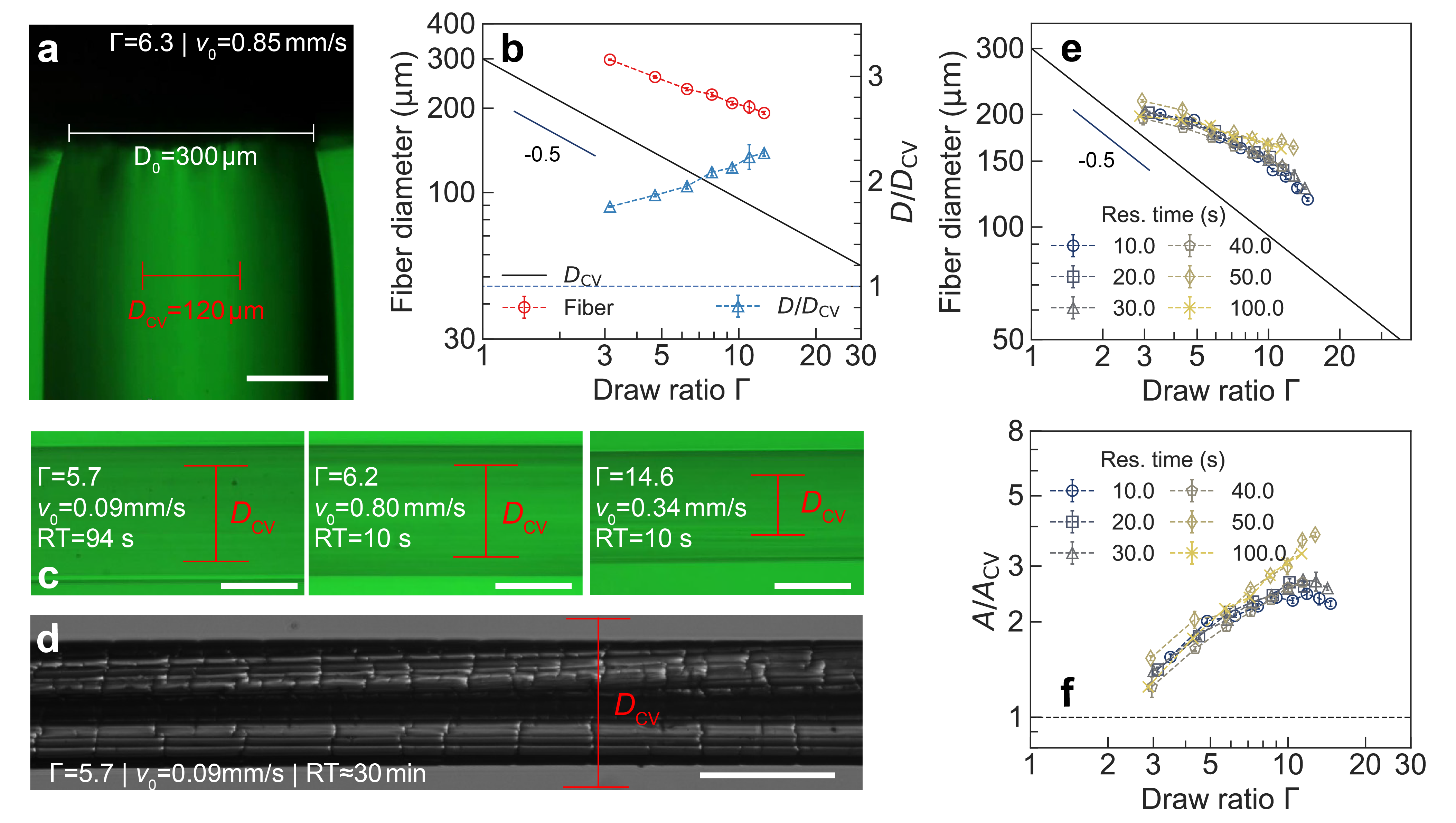
Figure 2: Evolution of fiber geometries in a spinning process. (a) Extruded filament near the spinneret that exhibits die-swelling effects. Draw ratio $\Gamma=6.3$. Red reference line: $D_{\mathrm{CV}}$. (b) Fiber diameter $D$ (red circles) and its ratio to that under conservation of volume $D/D_{\mathrm{CV}}$ (blue triangles) near spinneret ($x=$2\text{\,}\mathrm{m}\mathrm{m}$$) at varying draw ratios. Solid line: Predicted steady-state fiber diameter $D_{\mathrm{CV}}$ under conservation of volume. (c) Extruded filament sufficiently far from the spinneret ($x=$50\text{\,}\mathrm{m}\mathrm{m}$$) at varying draw ratios and residence times. Red reference line: $D_{\mathrm{CV}}$. (d) Bright-field image of a fully-coagulated fiber ($\Gamma=$5.7$$), showing spatially heterogeneous core-shell structures due to ongoing solvent/anti-solvent exchange. Red reference line: $D_{\mathrm{CV}}$. (e) Fiber diameter far from the spinneret against draw ratios at varying residence times. The spinneret diameter is fixed at $D_{0}=$300\text{\,}\mathrm{\SIUnitSymbolMicro m}\text{/}$$. (f) Fiber swelling ratio $A/A_{\mathrm{CV}}$ due to coagulation at varying draw ratios and residence time. Solid line: No change of fiber cross-section ($A=A_{\mathrm{CV}}$). Scale bars in (a), (c) and (d): $100\text{\,}\mathrm{\SIUnitSymbolMicro m}\text{/}$

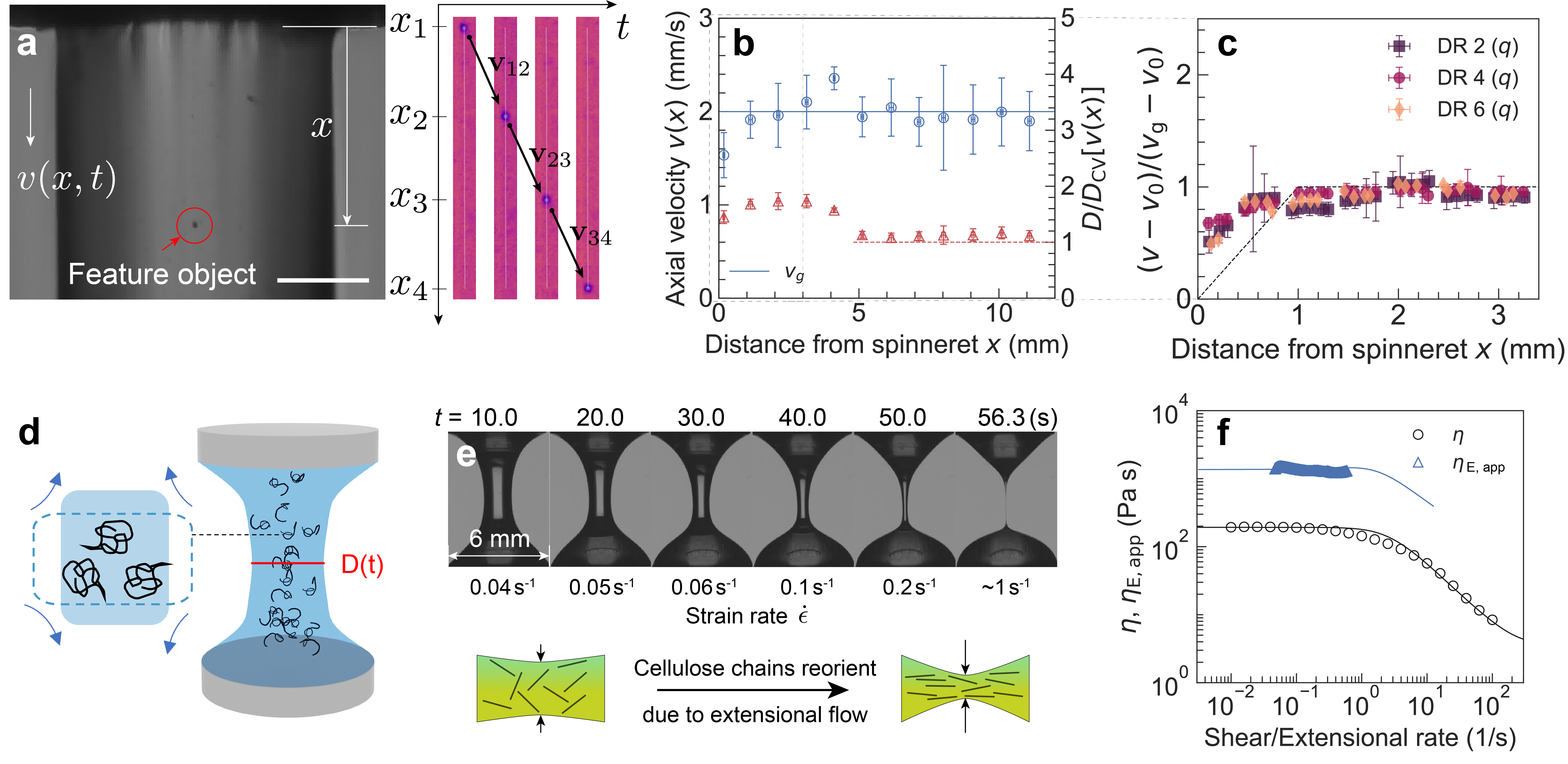
Figure 3: Velocimetry and rheological characterizations of the studied spinning dope. (a) Schematic of feature-tracking velocimetry at varying distance to the spinneret $x$. (b) Blue circles (left $y$-axis): Averaged axial velocity extracted from tracking multiple feature objects ($0\text{\,}\mathrm{m}\mathrm{m}$ to $11\text{\,}\mathrm{m}\mathrm{m}$; bin size $1\text{\,}\mathrm{m}\mathrm{m}$) at $\Gamma=$2$$. Blue solid line: $v_{\mathrm{g}}$. Red triangles (right $y$-axis): Ratio of fiber diameter $D$ and the transient fiber diameter under conversation of volume $D_{\mathrm{CV}}[v(x)]$. Red dashed line: Reference line with no change in fiber volume (c) Normalized axial velocity from averaging the transient velocity measurements ($0\text{\,}\mathrm{m}\mathrm{m}$ to $3\text{\,}\mathrm{m}\mathrm{m}$; bin size $0.2\text{\,}\mathrm{m}\mathrm{m}$) with the godet wheel speed ($v_{\mathrm{g}}$) at varying draw ratios $\Gamma=$246$$. Dashed line: approximated kinematic evolution for spun fibers (Equation 2). (d) Schematic of capillarity-driven breakup extensional rheometry, in which an extensional flow drives polymer-chain deformation. (e) Snapshots of the filament evolution during capillarity-driven thinning. Maximum transient strain rate $\dot{\epsilon}$ is calculated for each snapshot at the necking region. Bottom: Schematic of flow-induced cellulose reorientation under an extensional flow as the strain rate increases. (f) Shear viscosity $\eta$ (black circles) and apparent extensional viscosity $\eta_{\mathrm{E,app}}$ (blue triangles) plotted against the corresponding strain rates. Black and blue solid lines correspond to the fitting lines from the Rolie-Poly model under the same constitutive parameters. Both shear and extensional rheological characterizations were performed at $80\text{\,}\mathrm{\SIUnitSymbolCelsius}\text{/}$.

Figure 2 shows the overall filament morphology under varying spinning configurations. In general, we noticed expanded fiber diameter at the spinneret outlet (Figure 2a). We measured the fiber diameter at $x=$2\text{\,}\mathrm{m}\mathrm{m}$$, where $x$ is the distance from the end of spinneret along the fiber direction, at different draw ratios imposed by a constant flow rate ($v_{0}=$0.85\text{\,}\mathrm{m}\mathrm{m}\mathrm{/}\mathrm{s}$$) from the spinneret but different godet wheel speeds. The extracted fiber diameter $D$ at varying draw ratios (red circles in Figure 2b) exhibit a negative power-law trend against the draw ratio, and the values exceed the predicted diameter based on conservation of volume $D_{\mathrm{CV}}=D_{0}/\sqrt{\Gamma}$ (solid line in Figure 2a and red reference line in Figure 2c and d; $D_{0}=$300\text{\,}\mathrm{\SIUnitSymbolMicro m}\text{/}$$), which can be attributed to both the die-swelling effect from the spinning dope that leads to a non-trivial radial normal stress, and the exchange of solvents and antisolvents. The ratio of $D/D_{\mathrm{CV}}$ (blue triangles) remains above unity and steadily increases with the draw ratios. When the fiber travels far from the spinneret, the normal stress component in the radial direction due to die-swelling effect rapidly relaxes (indicated in Figure 3b), and the fiber kinematics are progressively dominated by the specified spinning parameters. Figure 2c shows the snapshots of fiber morphology at $\Gamma=5.7,6.2and14.6$ and residence time of $10\text{\,}\mathrm{s}$ and $94\text{\,}\mathrm{s}$. The measured fiber diameter is significantly larger than the diameter under conservation of volume $D_{\mathrm{CV}}$ (red reference lines). Consequently, the exchange of solvents and anti-solvents result in a net flow into the filament. In addition to the overall change in the fiber volume, the spatial distribution of different components is radially heterogeneous due to relatively low solvent/anti-solvent diffusivity in the coagulation process. This non-uniformity radial profile can be visualized by observing the fully-coagulated fiber ($\Gamma=$5.7$$) under brightfield imaging (Figure 2d), in which a core-shell structure can be clearly identified. Similar fiber structures have been characterized in a number of previous studies ^{26, 9}. We plotted the fiber diameters at varying draw ratios and resident times (Figure 2e). At different residence times, the evolution of fiber diameters broadly overlap and progressively grow beyond the reference diameter $D_{\mathrm{CV}}$ (black line) as the draw ratio increases. Of special note, the diameter of fully-coagulated fiber significantly decreases below that under conservation of volume (Figure 2d). As a result, we justified the change of fiber diameter in a coagulation process primarily attributed from the solvent/anti-solvent exchange. More quantitatively, the swelling ratios $A/A_{\mathrm{CV}}=(D/D_{\mathrm{CV}})^{2}$ can be calculated under the assumption that the fiber swells uniformly along the radial direction (Figure 2f). From the figure, the degree of fiber swelling in a coagulation process is largely dominated by the draw ratio.

From Figure 2, the fiber geometries in a spinning process deviate significantly from the predictions under conservation of volume. Consequently, the fiber kinematics cannot be inferred faithfully from the evolution of its diameter. Therefore, we performed feature-tracking velocimetry using the disperse phases in spinning dopes (Figure 3a). These features are largely resulted from the partially-dissolved cellulose with a typical size ranging from $10\text{\,}\mathrm{\SIUnitSymbolMicro m}\text{/}$ to $100\text{\,}\mathrm{\SIUnitSymbolMicro m}\text{/}$. While ionic-liquid solvents can dissolve native cellulose at concentrations above $15\text{\,}\%$, the preparation process requires delicate pretreatments at scaled-up production to facilitate dissolution with controllable derivatizing effects ²⁷. As a result, spinning dopes with partially-dissolved cellulose can better represent the material systems used for industrial applications ¹⁶. We justified that these disperse features can be used for particle-tracking velocimetry (PTV) by calculating the Stokes numbers defined as $\mathrm{St}=\tau_{\mathrm{i}}/\tau_{\mathrm{f}}$. Here, $\tau_{\mathrm{i}}$ is the relaxation time of a feature object in a flow field and is calculated from $\tau_{\mathrm{i}}=\rho_{\mathrm{i}}d_{\mathrm{i}}^{2}/(18\eta)$, where $\rho_{\mathrm{i}}$ and $d_{\mathrm{i}}$ are the density and diameter of the feature object, respectively, and $\eta$ is the viscosity of the fluid phase. On the denominator, $\tau_{\mathrm{f}}=d_{\mathrm{i}}/U_{0}$ characterizes the time of flow past the feature object, and $U_{0}$ is the field velocity. We calculated the Stokes number for a typical spinning process to be $\mathrm{St}=$1\text{\times}{10}^{-10}1\text{\times}{10}^{-8}$\ll 1$ based on independent measurements of the material properties, justifying the use of feature objects as tracers. To recover the axial velocity along the spinning direction, we sampled multiple feature objects at different distance $x=$0\text{\,}\mathrm{m}\mathrm{m}$to{11}{mm}$ from the spinneret, and calculated the ”transient” axial velocity of each feature object from two adjoining frames (Figure 3a). The image processing is performed by a third-party computation package trackpy ²⁸. We measured the axial velocity at $\Gamma=2$ at different locations and averaged the raw data into specified bin sizes ($1\text{\,}\mathrm{m}\mathrm{m}$) for plot legibility (Figure 3b). We noticed the fiber accelerated to the godet wheel speed $v_{\mathrm{g}}$ (blue solid line) within a short distance ($x\approx$1\text{\,}\mathrm{m}\mathrm{m}$$). A closer look in the range of $0\text{\,}\mathrm{m}\mathrm{m}$ to $3\text{\,}\mathrm{m}\mathrm{m}$ at varying draw ratios substantiates a consistent ”acceleration length” $L_{0}\approx$1\text{\,}\mathrm{m}\mathrm{m}$$ independent of the imposed draw ratios. As a result, the kinematics of extruded spinning dopes in a generic cellulose-fiber spinning process can be approximated as a piece-wise process: When $x<L_{0}$, the fiber is extended rapidly to reach the desired terminal velocity ($v_{\mathrm{g}}$), during which an extensional strain of $\epsilon_{0}=\ln{\Gamma}$ is accumulated. Beyond this acceleration period, the fiber moves broadly as a rigid body and undergoes a coagulation process over an extended time period. We further justified this separable accelerating-coagulation process via the distinct times for acceleration (approximately $1\text{\,}\mathrm{s}$) and diffusion (approximately $100\text{\,}\mathrm{s}$), the latter of which is calculated based on the diffusivity measurements during solvent/anti-solvent exchanges from a number of previous studies^{27, 29}. Because the kinematics evolve much faster than the diffusion, the deformation of fibers is relatively instantaneous compared with their regeneration through solvent/anti-solvent exchange.

To understand the dynamics of spinning dopes prior to the onset of regeneration, we performed comprehensive rheological characterizations to the spinning dope under both shear and extensional flows, which incorporate the deformation in the spinneret and during the spinning process, respectively. The shear rheology was measured using a commercial rheometer (Physica MCR 101, Anton Paar), and the extensional rheology was characterized using a customized capillarity-driven breakup extensional rheometer (CaBER) ²⁷. Both measurements were performed at $80\text{\,}\mathrm{\SIUnitSymbolCelsius}\text{/}$. The CaBER works by rapidly imposing an extensional strain to a fluid sample that rests between two coaxial plates, which induces filament pinch-off as a result of the driving surface tension and resistance from the material. An apparent extensional viscosity can thus be calculated from the measured filament diameter $D(t)$ (Figure 3d) as $\eta_{\mathrm{E,app}}=\sigma_{\mathrm{sd}}/[-\dot{D}(t)]$, where $\sigma_{\mathrm{sd}}$ is the surface tension of the spinning dope ($47\text{\,}\mathrm{m}\mathrm{N}\mathrm{/}\mathrm{m}$ ^{30, 23}). The snapshots of the filament show a breakup time of approximately $57\text{\,}\mathrm{s}$, during which the transient strain rates in the necking region of the filament increase from 0.04 to 1 $s^{-1}$ (Figure 3e). In this process, the cellulose chains are forced to reorient and the material properties are significantly modified. Finally, the extracted shear and apparent extensional viscosities are plotted and compared (Figure 3f). The spinning dope shows rate-thinning behavior in both shear and extensional flows. To extract the structural evolution during the flow deformation, we applied a physical constitutive model (Rolie-Poly model) to fit the experimental data in both shear and extensional flows following identical procedures in the previous study³⁰ (solid and dashed lines in Figure 3f). The fitting lines are in excellent agreement with the experimental data.

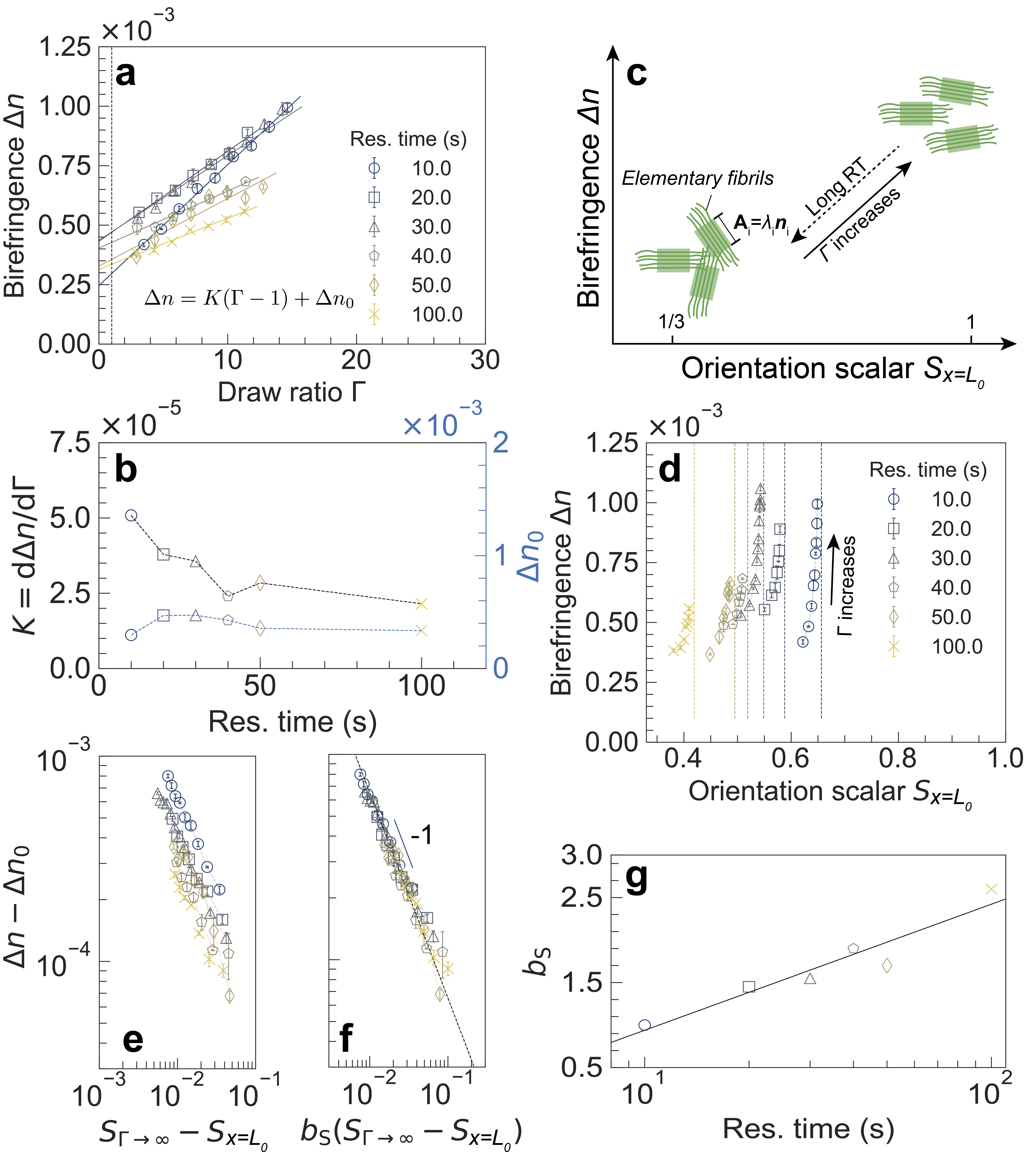
Figure 4: Online birefringence measurement of the fibers during coagulation process and structural interpretations from complex rheology. (a) Birefringence measurements of the fiber in coagulation at varying draw ratios and residence time. Solid lines: Linear fitting lines for each fixed residence time. Dashed vertical line: Draw ratio $\Gamma=1$. (b) Extracted fitting parameters of Equation 1 from (a). (c) Illustration of cellulose chain structures at different orientation scalars under varying spinning conditions. (d) Birefringent responses against peak orientation scalar $S(x=L_{0})$ at varying residence time. Dashed vertical line: Peak orientation scalar $S_{x=L_{0}}$ in the limit of $\Gamma\rightarrow\infty$. (e) Birefringent responses due to drawing, $(\Delta n-\Delta n_{0})$ against the orientation scalar difference, $(S_{\mathrm{\Gamma\rightarrow\infty}}-S_{x=L_{0}})$. (f) Birefringent responses due to drawing against $b_{\mathrm{S}}(S_{\mathrm{\Gamma\rightarrow\infty}}-S_{x=L_{0}})$, pivoted at the residence time of $10\text{\,}\mathrm{s}$. (f) Extracted horizontal shifting factor $b_{\mathrm{S}}$ against residence time with the abscissa plotted on logarithmic scale. Solid line: Linear fitting line of the extracted data.

The predicted structural evolution from the measured spinning dope kinematics and rheological responses is subsequently compared with the in situ birefringence measurements of fibers in a spinning process using an alternating LC retarder. Briefly, the LC retarder generates a series of retardation within half the wavelength, which is subsequently superposed to the unknown birefringent fibers. The birefringence measurement is obtained by extracting the phase difference between the evolution of light intensity with or without fibers. Because the phase difference is independent of the overall brightness, such birefringence measurements apply semi-opaque material systems as well. Using this measuring technique, we found the measured fiber birefringence to increase consistently with draw ratios at varying residence times (Figure 4a), showing primary birefringence contributions from fiber extension. We subsequently fit the evolution of birefringence with a linear relationship expressed as

$$\Delta n=K(\Gamma-1)+\Delta n_{0},$$ (1)

where $\Delta n_{0}$ is the intercept of birefringence in the absence of extension ($\Gamma=1$, vertical dashed line). The fitted values (blue squares) remain broadly constant, while the slope $K=\mathrm{d}\Delta n/\mathrm{d}\Gamma$ (black triangles) decreases as the residence time increases (Figure 4b). The constant non-zero intercept in the absence of extension can be attributed to the non-trivial residue cellulose alignment during the flow in spinneret, which remains unaffected during the regeneration process. As we attribute the variations in birefringence to the flow-induced anisotropic structures resulted from the reorientation of semi-flexible cellulose chains under drawing process, the decreased slope $K$ at increased residence time represents enhanced resistance to a preferred cellulose alignment under external drawing as the fibers are increasingly coagulated, partially due to enhanced fiber stiffness and cellulose relaxation. In contrast, the birefringent responses of spun fibers are largely determined during the extensional deformation of spinning dopes, parameterized by the draw ratios. Figure 3 has shown that such extensional deformation is imposed in a short acceleration length $L_{0}$ when the majority of the filament remains uncoagulated. As a result, the structural properties of the spun fiber at $x=L_{0}$ can be largely inferred from the rheology of spinning dope using previously measured flow kinematics, and become an accessible property indicator that readily connects to the fully-coagulated fibers. Quantitatively, an orientation tensor $\mathbf{W}$ is commonly used to describe the ensemble-averaged orientation of Kuhn steps of all the polymer chains in a solution, and has been integrated into a number of constitutive models based on kinetic theories to connect micro- and macroscopic properties for polymer solutions and polymer melts ^{31, 25}. Specifically, Owens et al. ³⁰ has applied the Rolie-Poly model to derive a unified mechanical framework to describe the flow behavior of cellulose dissolved in ionic liquids over a wide range of strain rates. A frame-invariant scalar can be derived from the double-dot product $S=\mathbf{W}:\mathbf{W}$ to describe the macroscopic anisotropy arising from preferred orientation of polymer-chain ensembles, where $S=1/3$ corresponds to a randomly-oriented distribution, whereas $S=1$ corresponds to a well-aligned distribution ³² (Figure 4c). In a spinning process, the evolution of $\mathbf{W}$ can be calculated from the measured flow kinematics in the form of axial velocity $v(x)$. To demonstrate this relationship, we approximate the evolution of axial velocity in a coagulation process using a simple linear form (dashed line in Figure 3c) as

$$v(x)=\begin{cases}v_{0}+\dfrac{(v_{\mathrm{g}}-v_{0})x}{L_{0}},&x\leq L_{0}\\ v_{\mathrm{g}},&x>L_{0}\\ \end{cases}$$ (2)

where $L_{0}$ is the acceleration length measured in Figure 3. The imposed strain rate during fiber acceleration remains constant and can be calculated as $\dot{\epsilon}(x)=\mathrm{d}v/\mathrm{d}x=(v_{\mathrm{g}}-v_{0})/L_{0}$ for an extended period of $t_{\mathrm{a}}=\int_{0}^{L_{0}}\mathrm{d}x/v=L_{0}\ln{(\Gamma)}/(v_{\mathrm{g}}-v_{0})$. The transient extensional rate $\dot{\epsilon}(x)$ can thus be substituted into the constitutive equation to calculate the evolution of orientation tensor $\mathbf{W}(x)$. The initial condition ($x=0$ in a Eulerian frame) is inferred from the steady-state shear flow in the spinneret based on the imposed flow rate and the spinneret geometry. By plotting the measured birefringence against a peak orientation scalar $S_{x=L_{0}}$ defined at $x=L_{0}$ for each residence time (Figure 4d), we identified similar increasing trends in the birefringence as the structure becomes more aligned. Compared with the imposed spinning parameters, the birefringence provides a more generic and consolidated measure for the resulting fiber structure. To show this, we establish a superposing relationship between the birefringence and the structural parameters under varying spinning conditions. We notice that at a fixed residence time (hence $v_{\mathrm{g}}$), the peak orientation scalar converges to a finite value $S_{\Gamma\rightarrow\infty}$ as the draw ratio increases. This finite value can be determined by imposing a steady-state extensional rate of $\dot{\epsilon}=v_{\mathrm{g}}/L_{0}$, which can be shown to produce a mathematically equivalent flow dynamic (dashed vertical asymptotes in Figure 4d). We identified similar asymptotic trends of birefringence measurements at different residence time. To render a superposed relationship across varying residence times, we replotted the birefringence due to spinning, $\Delta n-\Delta n_{0}$, against $S_{\Gamma\rightarrow\infty}-S_{x=L_{0}}$ (Figure 4e). We found that all curves exhibit a power-law decaying trend with a broadly constant power exponent of $-1$. A horizontal shifting factor $b_{\mathrm{S}}$ based on the measurement at residence time of $10.0\text{\,}\mathrm{s}$ is imposed to further consolidate a master curve at varying residence time (Figure 4f), and the shifting factor $b_{\mathrm{S}}$ extracted from the least square regression exhibits a clear correlation with the residence time (Figure 4g). The last shifting operation is not trivial, because the rate of relaxation for cellulose orientation can vary significantly with the residence time, and needs to be described separately with an additional superposition. The extracted shifting factor $b_{\mathrm{S}}$ appears to be proportional with the logarithmic residence time (black line), which indicates a slow-down in cellulose relaxation as the residence time increases. As a result, we justify a universal rheo-optic relationship derived from the general constitutive model for entangled spinning dopes using the peak orientation scalar. Of special note, the birefringence of cellulose fibers is not only function of the draw ratio and the residence time, but also of the extrusion speed at the spinneret, which dominates the cellulose orientation under rapid extension at the onset of fiber spinning. The mechanical properties of fully-coagulated fibers thus vary accordingly, even if the draw ratios are identical.

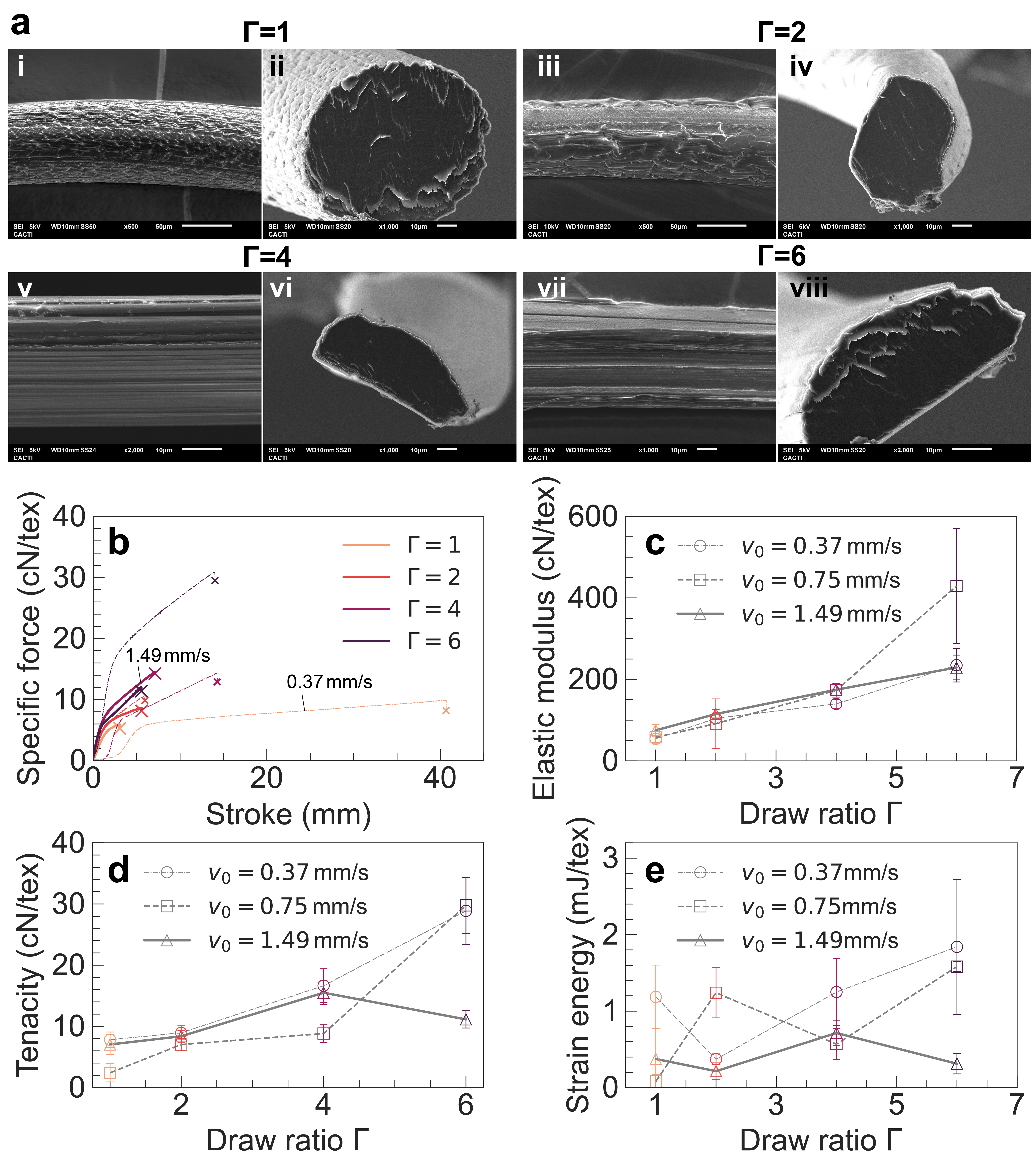
Figure 5: Structural and mechanical characterizations of fully-coagulated fibers. (a) Scanning electron microscopic images of longitudinal (i, iii, v, vii) and cross-sectional (ii, iv, vi, viii) views of the spun fibers at varying draw ratios and extrusion speed of $v_{0}=$0.75\text{\,}\mathrm{m}\mathrm{m}\mathrm{/}\mathrm{s}$$. Scale bars are specified in each image. (b) Specific force-stroke curve for fully-coagulated fibers generated at varying draw ratios ($\Gamma=1,2,4,6$) and extrusion speeds ($v_{0}=$0.37\text{\,}\mathrm{m}\mathrm{m}\mathrm{/}\mathrm{s}$to$1.49\text{\,}\mathrm{m}\mathrm{m}\mathrm{/}\mathrm{s}$$). One dataset under each condition is shown. The points of failure are marked in each curve. (c) Measures of modulus for fully- coagulated fibers against draw ratios at varying extrusion speeds ($v_{0}=0.37,0.75,$1.49\text{\,}\mathrm{m}\mathrm{m}\mathrm{/}\mathrm{s}$$), extracted from the maximum slope of the specific force-stroke curves. (d) Measures of tenacity for fully-coagulated fibers against draw ratios at varying extrusion speeds ($v_{0}=0.37,0.75,$1.49\text{\,}\mathrm{m}\mathrm{m}\mathrm{/}\mathrm{s}$$), extracted from the maximum specific force prior to points of failure. (e) Measures of specific strain energy against draw ratios for fully-coagulated fibers at varying extrusion speeds ($v_{0}=0.37,0.75and$1.49\text{\,}\mathrm{m}\mathrm{m}\mathrm{/}\mathrm{s}$$), calculated from integrating the specific force-stroke curve in (b) before points of failure. Three tests were performed for each datapoint in (c), (d) and (e).

The spun fibers under varying spinning condition were collected from the miniature spinline, fully coagulated and dried for structural and mechanical characterizations (Figure 5). Longitudinal (i, iii, v, vii) and cross-sectional (ii, iv, vi, viii) morphologies at varying draw ratios ($\Gamma=$1246$$ at $v_{0}=$0.75\text{\,}\mathrm{m}\mathrm{m}\mathrm{/}\mathrm{s}$$) were captured from scanning electron microscopy (Figure 5a; JEOL USA), and stronger extension in the drawing direction can be identified as the draw ratio increases. The fiber cross-sections at high draw ratios are smoother and progressively deviate from circular shapes, which are compatible deformations caused by the horizontal rods in the coagulation bath (see experimental setup in Figure 1) induced by the strain in the take-over rod (Godet wheel), demonstrating increased plasticity due to enhanced cellulose alignment. The mechanical properties of the fully-coagulated fibers were measured using a standard mechanical tester (AGS-X STD, Shimadzu) equipped with a $10\text{\,}\mathrm{N}$-load cell according to the standard measuring protocol ³³. To substantiate the effects from both draw ratios and extrusion speeds on the spinning performance, three extrusion speeds ($v_{0}=0.37,0.75,$1.49\text{\,}\mathrm{m}\mathrm{m}\mathrm{/}\mathrm{s}$$) were tested. Figure 5b shows specific force against stroke at distinct extrusion speeds of $0.37\text{\,}\mathrm{m}\mathrm{m}\mathrm{/}\mathrm{s}$ (thin dashed lines) and $1.49\text{\,}\mathrm{m}\mathrm{m}\mathrm{/}\mathrm{s}$ (thick solid lines) at varying draw ratios. We identified similar two-stage mechanical responses with elastic and plastic regions under varying spinning conditions. However, the magnitudes on both abscissa and ordinate show distinct trends. To quantify the mechanical responses of the spun fibers, three specific properties were extracted from the force-stroke curve: the stiffness, the tenacity, and the strain energy (Figure 5e). The stiffness, which describes the linear elasticity, increases at a higher draw ratio, but remains broadly unchanged at varying extrusion speeds (Figure 5c). Beyond the linear region, the tenacity and strain energy, which describe the fiber strength and toughness, respectively, increase at a higher draw ratio as well as at a slower extrusion speed. For an entangled polymer network such as regenerated cellulose fibers, the linear elasticity arises from variations in microscopic entropy due to reorientation of cellulose chains ²⁵. As a result, the magnitude of elastic moduli is readily connected to the structural conformation after spinning, regardless of the transient deformation throughout the process. Figure 4b, the birefringence measurement under no extension ($\Delta n_{0}$) is broadly constant across varying residence times. As result, the structural conformation of the regenerated cellulose is largely determined by the draw ratio, hence the linear elastic properties. On the contrary, despite a number of studies that have addressed the dependence of tenacity on draw ratio ^{9, 34}, these non-linear mechanical properties appear to be functions of the extrusion speed $v_{0}$ as well. The enhanced tenacity and specific strain energy at lower extrusion speeds have been briefly reported previously ^{35, 36}, which attributed the more tenacious and ductile trends in the regenerated fibers at lower extrusion speeds to a smaller deformation rate in the spinneret, thus less deformation energy in the spinning-dope before spinning and coagulation. However, as stated previously, we did not observe significant change in the birefringence of spinning dope right after extrusion from the spinneret at $\Gamma=1$ ($\Delta n_{0}$ in Figure 4b). As a result, we attribute the increased tenacity and toughness to the prolonged acceleration time $t_{\mathrm{a}}$ during the fiber drawing period ($x<L_{0}$) as the extrusion speed decreases at a constant draw ratio. By substituting the spinning parameters, we found that such acceleration times under all the studied spinning conditions are greater than $0.24\text{\,}\mathrm{s}$, which remains larger than the disengagement time ($\tau_{\mathrm{d}}\approx$0.21\text{\,}\mathrm{s}$$) in the Rolie-Poly model extracted from the rheological characterizations (Figure 3f). As a result, despite the fiber drawing induced by a non-trivial draw ratio, which induces significant reorientation to the cellulose chains via advection, these chains simultaneously undergo a disengaging process and are reorganized to reduce the free energy. This “annealing-like” process homogenizes the microstructures and gives rise to enhanced resistance to material failure at larger external deformation, and is critical to grant strong and tough fibers that may find commercial applications.

3 Conclusions

In this work, we propose a universal rheo-optic framework to monitor the regeneration process for cellulose dissolved in ionic liquids via a wet-spinning. A mini-spinline was constructed and integrated with a polarized microscope to visualize the geometry and birefringence of spun cellulose fibers in real time at varying draw ratios and residence times. Using feature tracking techniques, we identified a broadly constant distance within which the fibers are extended upon extrusion from the spinneret. Beyond this point, the fibers move in the coagulation bath with minimal deformation for an extended period (residence time), where the exchange of solvents and anti-solvents gradually regenerates the cellulose network.

We measured the birefringence of fibers in the spinning process to substantiate the microstructural variation. To quantify the flow-induced structural evolution during the spinning process, a rheo-optic framework based on the Rolie-Poly model was proposed, and the constitutive parameters were extracted from independent shear and extensional rheological characterizations. Based on this rheo-optic framework, a superposing relationship can be obtained between the optical measurements and the inferred structural anisotropy, hence providing accessible indicators of the cellulose structures from online birefringence measurements.

Finally, the mechanical properties of regenerated fibers at varying draw ratios and extrusion speeds were measured. While the linear elastic properties appear to be sole functions of the draw ratio, we identified enhanced tenacities and strain energies as the extrusion speed decreased. We attributed this trend in the non-linear region to the lower transient anisotropy of cellulose structures throughout the spinning process, which allows for enhanced degree of structural relaxation. As a result, the coagulation process is more homogenized to reduce the free energy of formed cellulose chains, and to facilitate the growth of larger cellulose networks.

4 Experimental Section

4.1 Material preparations

The material system applied in this work is prehydrolysis-kraft dissolving pulp (Eucalyptus urograndis, 93% cellulose I, $M_{\mathrm{w}}=$269\text{\,}\mathrm{k\text{Da}}\text{/}$$ and $M_{\mathrm{n}}=$79\text{\,}\mathrm{k\text{Da}}\text{/}$$ with a polydispersity of $3.4$) dissolved in 1-ethyl-3- methylimidazolium acetate ([C2C1Im][OAc]) provided through courtesy of Prof. Michael Hummel from Aalto University. The concentration is selected at $5\text{\,}\mathrm{\text{wt\%}}\text{/}$ (corresponding to $c/c_{\mathrm{e}}\approx 2.5$, where $c_{\mathrm{e}}$ is the entanglement concentration). Material systems with $c>c_{\mathrm{e}}$ are selected to be consistent with real spinning processes, in which concentrated cellulose spinning dopes are generally applied ⁹. Spinning dopes were prepared following a standard procedure that has been illustrated elsewhere ³⁰. Briefly, a certain amount of cellulose was dissolved at $90\text{\,}\mathrm{\SIUnitSymbolCelsius}\text{/}$, in a glass beaker sealed with a PTFE stirrer bearing under mechanical mixing for $60\text{\,}\mathrm{m}\mathrm{i}\mathrm{n}\mathrm{s}$. After complete dissolution dopes where filtered at room temperature through a $7\text{\,}\mathrm{\SIUnitSymbolMicro m}\text{/}$-filter mesh and degassed at $70\text{\,}\mathrm{\SIUnitSymbolCelsius}\text{/}$.

4.2 Customized spin-line with in situ birefringence measurement

A customized spin-line was constructed (Figure 1a), in which the spinning dope is extruded from a custom designed spinneret with the nozzle diameter of $300\text{\,}\mathrm{\SIUnitSymbolMicro m}\text{/}$. The extruded dope undergoes the coagulation process in an aqueous bath as antisolvent between two pillars of an identical size. The fibers, after a fixed time of residence are subsequently reeled with a godet wheel and collected for post factum characterizations. During the spinning and coagulation process, the spinning dope undergoes extensional deformation along the spinning direction. As antisolvent diffuses into the dope and induces the gelation of crystalline cellulose, an overall orientation of the cellulose structure is induced. Due to the resulting anisotropy in the overall structure, birefringent responses are generated (Figure 1a:1-2), where the slow axis points in the spinning direction. To quantify the birefringent responses, an optical setup (Figure 1b) derived from the work of Honda et al. ³⁷ was constructed. Here, a collimated light (SOLIS-525A, Thorlabs) with a mean wavelength of $525\text{\,}\mathrm{nm}\text{/}$ is incident through a polarizer with its slow axis configured at $45\mathrm{°}$ with the horizontal plane. Another analyzer is set with the slow axis set at $-45\mathrm{°}$ against the horizontal plane. Between the polarizer and analyzer, the fiber to be measured is set within the light beam range. To allow for calibrated real-time measurements, a liquid-crystal (LC) retarder is installed long the optical path with the slow axis set at $0\mathrm{°}$.

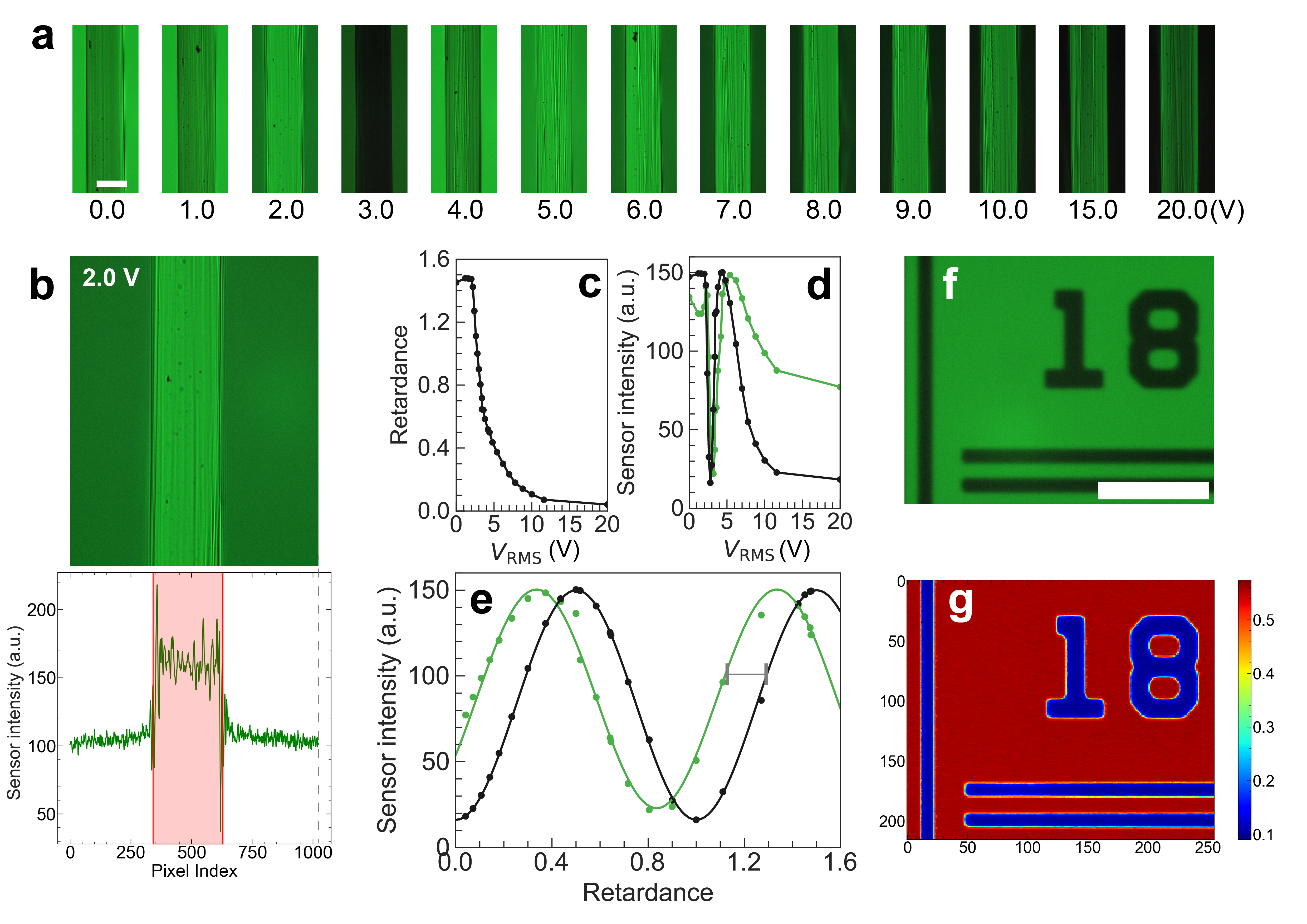
Figure 6: Method overview for fiber detection and birefringence measurement at $\Gamma=11.4$ and residence time of $39\text{\,}\mathrm{s}$. The wavelength of monotonic light source is $525\text{\,}\mathrm{n}\mathrm{m}$. (a) Snapshots of extruded fibers captured at different root mean square (RMS) voltage levels from the LC retarder. (b) Edge detection for extruded fibers with non-smooth surfaces. Top: Snapshot of the extruded fiber at voltage of $2\text{\,}\mathrm{V}$ from the LC retarder. Bottom: Extracted sensor intensity along cross- sectional direction averaged in the longitudinal direction. (c) Calibration curve of retardance for the applied LC retarder. (d) Measured image sensor intensity for the extruded fiber (green) and the background (black) at different RMS voltages. (e) Measured image sensor intensity for the fiber (green) and the background (black) at varying LC retardance. (f) Test birefringent target at $V_{\mathrm{RMS}}=$0\text{\,}\mathrm{V}$$. (g) Extracted retardance from the test birefrigent target in (f). Scalebars in (a) and (f) are $100\text{\,}\mathrm{\SIUnitSymbolMicro m}\text{/}$.

In a birefringence measurement, a well-modulated voltage profile is provided to the LC retarder, which induces a temporally-evolving predetermined birefringence along the optical path. Such birefringence induced by the LC-retarder superposed with the intrinsic birefringence from the sample results in alternating bright-dark image snapshots at different root mean square (RMS) voltage levels (Figure 6a). The net optical retardance from the fiber can be determined by subtracting the measured retardance in the background from that at the fiber centerline. The fiber birefringence can be subsequently determined given the fiber geometry. We implemented a simple scheme to determine the fiber edges by locating the maximal image gradient along a cross-sectional cut line (Figure 6b). Subsequently, the fiber centerline and the background regions can be identified. Of note, some LC retarder voltage values are insufficient to generated highly-contrasted background-fiber interface, leading to an incorrect estimation of the fiber diameter. To correct such miscalculation, the recorded measurement for fiber diameter is taken as the median measurement over a cycle of voltage iteration from the LC retarder.

For simplified calculation, we assumed negligible reflectance and absorbance for the polarizers. Given the previously-stated slow-axis orientations for all the optical components, the resulting light transmittance (dimensionless) is given by Equation 3 as

$$T_{\Delta\phi}=\dfrac{I_{\mathrm{\Delta\phi}}}{I_{0}}=\sin^{2}(\pi\Delta\phi)=\sin^{2}(\pi\Delta nd/\lambda),$$ (3)

where $\Delta\phi=\phi_{\mathrm{f}}-\phi_{\mathrm{LC}}=(\Delta n_{\mathrm{f}}-\Delta n_{\mathrm{LC}})D/\lambda$ is the dimensionless retardance difference between the fiber sample and the LC retarder at an incident light wavelength $\lambda$. The birefringence of the fiber sample and the LC retarder are $\Delta n_{\mathrm{f}}$ and $\Delta n_{\mathrm{LC}}$, with the optical path lengths identical to the fiber diameter $D$ and the LC retarder thickness, respectively.

From the LC retarder, its retardance $\phi_{\mathrm{LC}}(V_{\mathrm{RMS}})$ is a function of the input voltage, $V_{\mathrm{RMS}}$ (Figure 6c, provided by the manufacturer). We note that in the accessible range of the retardance, the transmittance of the LC retarder $T_{\Delta\phi}$ is non-monotonic regarding to $V_{\mathrm{RMS}}$ (black line in Figure 6d), as well as when superposed with the birefringent fiber (green line in Figure 6d). The two measured image intensities are subsequently plotted against retardance using an interpolated form of the retardance calibration curve (Figure 6e; black: LC retarder; green: LC retarder superposed with fiber; gray scale: phase difference). The two image intensity responses exhibit periodical patterns with a non-trivial phase difference. From Equation 3, the light intensity follows a sinusoidal form regarding to the LC retardance $\phi_{\mathrm{LC}}$ as

$$I_{\Delta\phi}(\phi_{\mathrm{LC}})=\dfrac{1-\cos[2\pi(\phi_{\mathrm{f}}-\phi_{\mathrm{LC}})]}{2}I_{0}.$$ (4)

In practice, the numerical intensity extracted from the image pixels slightly deviates from a sinusoidal form due to its non-linear correlation with the light intensity. Nevertheless, a phase difference between the two periodical patterns can still be identified via numerical fitting of a sinusoidal function $f(\phi)=A\sin[2\pi(\phi+B)]+C$, where $A$, $B$ and $C$ are the fitting parameters. Finally, the difference in the values of $B$ coincides with the retardance of the fiber.

Acknowledgements

P.O. and P.B.S. were supported by Ministerio de Ciencia e Innovación under the grants PRE2020-093158 and RYC2021-033826-I respectively. J.D. and P.B.S thank Crystal Owens and Prof. Gareth H. McKinley from MIT for the insightful discussions.

Conflict of Interest

The authors declare no conflict of interest.

Data Availability Statement

The data that support the findings of this study are available from the corresponding author upon reasonable request.

References

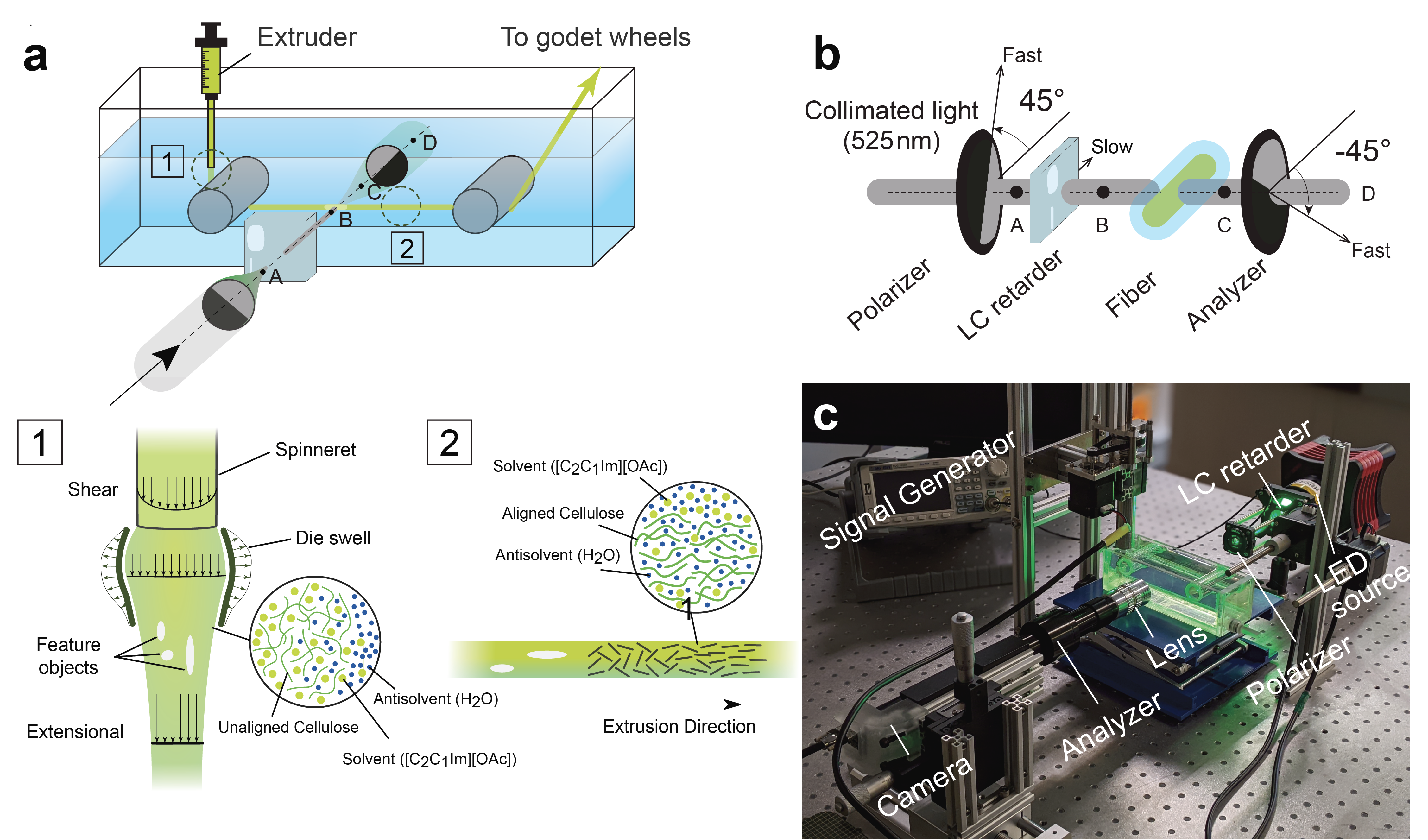
Figure 1: Configuration for in situ birefringence measurement on a miniature spinline. (a) Overview of the experimental setup, which constitutes a customized miniature spinline and necessary optical components for polarized microscopy. Schematics underneath show the kinematics and internal structures in the spun fibers (1) near and (2) far from the spinneret. (b) Components the polarized optical setup for birefringence measurement. Position A, B, C and D are consistent with notations in (a). (c) Real experimental setup with primary mechanical and optical components marked in text.

References

- Klemm et al. 2011 Klemm, D.; Kramer, F.; Moritz, S.; Lindström, T.; Ankerfors, M.; Gray, D.; Dorris, A. Nanocelluloses: A New Family of Nature-Based Materials. Angewandte Chemie International Edition 2011, 50, 5438–5466
- Fuller 1995 Fuller, G. G. Optical Rheometry of Complex Fluids; Oxford University Press, USA, 1995
- Oldenbourg et al. 2005 Oldenbourg, R., et al. Polarization microscopy with the LC-PolScope. Live cell imaging: A laboratory manual 2005, 205–237
- Mortimer and Peguy 1994 Mortimer, S. A.; Peguy, A. A Device for On-Line Measurement of Fiber Birefringence. Textile Research Journal 1994, 64, 544–551
- Mortimer and Péguy 1996 Mortimer, S. A.; Péguy, A. A. The Formation of Structure in the Spinning and Coagulation of Lyocell Fibres. Cellulose Chemistry and Technology 1996, 30, 117–132
- Mortimer et al. 1996 Mortimer, S. A.; Péguy, A. A.; Ball, R. Influence of the Physical Process Parameters on the Structure Formation of Lyocell Fibres. Cellulose Chemistry and Technology 1996, 30, 251–266
- Mortimer and Peguy 1998 Mortimer, S. A.; Peguy, A. Spinning of Fibres through the N-methylmorpholine-N-oxide Process. Use of Minerals in Papermaking 1998, 561–567
- Ma et al. 2019 Ma, Y.; Zeng, B.; Wang, X.; Byrne, N. Circular Textiles: Closed Loop Fiber to Fiber Wet Spun Process for Recycling Cotton from Denim. ACS Sustainable Chemistry & Engineering 2019, acssuschemeng.8b06166
- Hauru et al. 2014 Hauru, L. K. J.; Hummel, M.; Michud, A.; Sixta, H. Dry Jet-Wet Spinning of Strong Cellulose Filaments from Ionic Liquid Solution. Cellulose 2014, 21, 4471–4481
- Swatloski et al. 2002 Swatloski, R. P.; Spear, S. K.; Holbrey, J. D.; Rogers, R. D. Dissolution of Cellose with Ionic Liquids. Journal of the American Chemical Society 2002, 124, 4974–4975
- Welton 1999 Welton, T. Room-Temperature Ionic Liquids. Solvents for Synthesis and Catalysis. Chemical Reviews 1999, 99, 2071–2083
- Miyafuji 2015 Miyafuji, H. Application of Ionic Liquids for Effective Use of Woody Biomass. Journal of Wood Science 2015, 61, 343–350
- Brennecke and Maginn 2001 Brennecke, J. F.; Maginn, E. J. Ionic Liquids: Innovative Fluids for Chemical Processing. AIChE Journal 2001, 47, 2384–2389
- Plechkova and Seddon 2008 Plechkova, N. V.; Seddon, K. R. Applications of Ionic Liquids in the Chemical Industry. Chemical Society Reviews 2008, 37, 123–150
- De Silva and Byrne 2017 De Silva, R.; Byrne, N. Utilization of Cotton Waste for Regenerated Cellulose Fibres: Influence of Degree of Polymerization on Mechanical Properties. Carbohydrate Polymers 2017, 174, 89–94
- Hermanutz et al. 2019 Hermanutz, F.; Vocht, M. P.; Panzier, N.; Buchmeiser, M. R. Processing of Cellulose Using Ionic Liquids. Macromolecular Materials and Engineering 2019, 304, 1–8
- Han and Segal 1970 Han, C. D.; Segal, L. A Study of Fiber Extrusion in Wet Spinning. II. Effects of Spinning Conditions on Fiber Formation. Journal of Applied Polymer Science 1970, 14, 2999–3019
- Michud et al. 2016 Michud, A.; Tanttu, M.; Asaadi, S.; Ma, Y.; Netti, E.; Kääriainen, P.; Persson, A.; Berntsson, A.; Hummel, M.; Sixta, H. Ioncell-F: Ionic Liquid-Based Cellulosic Textile Fibers as an Alternative to Viscose and Lyocell. Textile Research Journal 2016, 86, 543–552
- Sayyed et al. 2019 Sayyed, A. J.; Deshmukh, N. A.; Pinjari, D. V. A Critical Review of Manufacturing Processes Used in Regenerated Cellulosic Fibres: Viscose, Cellulose Acetate, Cuprammonium, LiCl/DMAc, Ionic Liquids, and NMMO Based Lyocell. Cellulose 2019, 26, 2913–2940
- Kong and Eichhorn 2005 Kong, K.; Eichhorn, S. J. Crystalline and Amorphous Deformation of Process-Controlled Cellulose-II Fibres. Polymer 2005, 46, 6380–6390
- Mittal et al. 2018 Mittal, N.; Ansari, F.; Krishne, V. G.; Brouzet, C.; Chen, P.; Larsson, P. T.; Roth, S. V.; Lundell, F.; Wågberg, L.; Kotov, N. A.; Söderberg, L. D. Multiscale Control of Nanocellulose Assembly: Transferring Remarkable Nanoscale Fibril Mechanics to Macroscale Fibers. ACS Nano 2018, 12, 6378–6388
- Du 2022 Du, J. Advanced Rheological Characterization of Nanofilled Materials for Automotive Applications. Thesis, Massachusetts Institute of Technology, 2022
- Haward et al. 2012 Haward, S. J.; Sharma, V.; Butts, C. P.; McKinley, G. H.; Rahatekar, S. S. Shear and Extensional Rheology of Cellulose/Ionic Liquid Solutions. Biomacromolecules 2012, 13, 1688–1699
- Gericke et al. 2009 Gericke, M.; Schlufter, K.; Liebert, T.; Heinze, T.; Budtova, T. Rheological Properties of Cellulose/Ionic Liquid Solutions: From Dilute to Concentrated States. Biomacromolecules 2009, 10, 1188–1194
- Dealy and Larson 2006 Dealy, J. M.; Larson, R. G. Molecular Structure and Rheology of Molten Polymers; 2006
- Hedlund et al. 2017 Hedlund, A.; Köhnke, T.; Theliander, H. Diffusion in Ionic Liquid-Cellulose Solutions during Coagulation in Water: Mass Transport and Coagulation Rate Measurements. Macromolecules 2017, 50, 8707–8719
- Nazari et al. 2017 Nazari, B.; Utomo, N. W.; Colby, R. H. The Effect of Water on Rheology of Native Cellulose/Ionic Liquids Solutions. Biomacromolecules 2017, 18, 2849–2857
- Allan et al. 2021 Allan, D. B.; Caswell, T.; Keim, N. C.; van der Wel, Casper M.,; Verweij, R. W. Soft-Matter/Trackpy: Trackpy v0.5.0. Zenodo, 2021
- Hauru et al. 2016 Hauru, L. K. J.; Hummel, M.; Nieminen, K.; Michud, A.; Sixta, H. Cellulose Regeneration and Spinnability from Ionic Liquids. Soft Matter 2016, 12, 1487–1495
- Owens et al. 2022 Owens, C. E.; Du, J.; Sánchez, P. B. Understanding the Dynamics of Cellulose Dissolved in an Ionic Liquid Solvent Under Shear and Extensional Flows. Biomacromolecules 2022, 23, 1958–1969
- McLeish 2002 McLeish, T. C. B. Tube Theory of Entangled Polymer Dynamics. Advances in Physics 2002, 51, 1379–1527
- Likhtman and Graham 2003 Likhtman, A. E.; Graham, R. S. Simple Constitutive Equation for Linear Polymer Melts Derived from Molecular Theory: Rolie-Poly Equation. Journal of Non-Newtonian Fluid Mechanics 2003, 114, 1–12
- 33 14:00-17:00, ISO 5079:1995. https://www.iso.org/standard/11101.html
- Suzuki et al. 2021 Suzuki, S.; Togo, A.; Gan, H.; Kimura, S.; Iwata, T. Air-Jet Wet-Spinning of Curdlan Using Ionic Liquid. ACS Sustainable Chemistry & Engineering 2021, 9, 4247–4255
- Moriam et al. 2021 Moriam, K.; Sawada, D.; Nieminen, K.; Ma, Y.; Rissanen, M.; Nygren, N.; Guizani, C.; Hummel, M.; Sixta, H. Spinneret Geometry Modulates the Mechanical Properties of Man-Made Cellulose Fibers. Cellulose 2021, 28, 11165–11181
- Li et al. 2014 Li, X.; Li, N.; Xu, J.; Duan, X.; Sun, Y.; Zhao, Q. Cellulose Fibers from Cellulose/1-Ethyl-3-Methylimidazolium Acetate Solution by Wet Spinning with Increasing Spinning Speeds. Journal of Applied Polymer Science 2014, 131
- Honda et al. 2018 Honda, R.; Ryu, M.; Li, J. L.; Mizeikis, V.; Juodkazis, S.; Morikawa, J. Simple Multi-Wavelength Imaging of Birefringence:Case Study of Silk. Scientific Reports 2018, 8, 1–9