Probabilistic forecasting with Factor Quantile Regression: Application to electricity trading

Abstract

This paper presents a novel approach for constructing probabilistic forecasts, which combines both the Quantile Regression Averaging (QRA) method and the Principal Component Analysis (PCA) averaging scheme. The performance of the approach is evaluated on datasets from two European energy markets - the German EPEX SPOT and the Polish Power Exchange (TGE). The results indicate that newly proposed solutions yield results, which are more accurate than the literature benchmarks. Additionally, empirical evidence indicates that the proposed method outperforms its competitors in terms of the empirical coverage and the Christoffersen test. In addition, the economic value of the probabilistic forecast is evaluated on the basis of financial metrics. We test the performance of forecasting models taking into account a day-ahead market trading strategy that utilizes probabilistic price predictions and an energy storage system. The results indicate that profits of up to 10 EUR per 1 MWh transaction can be obtained when predictions are generated using the novel approach.

1 Introduction

Energy and, in particular, electricity markets are crucial for global and local economies. They are, on the one hand, exposed to various risks associated with various uncertainty sources (Wang et al., 2022), political decisions and international conflicts and, on the other hand, they have an important impact on all types of human activity (Churchill et al., 2022; Huntington and Liddle, 2022). Therefore, modeling and forecasting of electricity markets: the demand level, the supply structure, and the level of prices are of interest to many researchers and practitioners (Jåstad et al., 2022). In the literature, there are many articles that focus on point predictions of electricity prices (see Weron (2014) for a comprehensive review). However, recent publications (Hong et al. (2020); Nowotarski and Weron (2018); Janczura and Wójcik (2022)) and the wide interest in the 2014 Global Energy Forecasting Competition (GEFCom2014) demonstrate that there is a need for more comprehensive approaches, such as probabilistic forecasting. A precise approximation of the predictive distribution of the electricity price overcomes the limitations of point forecasts and allows for a better risk management (precise estimation of Value-at-Risk of the energy portfolio; Bunn et al. (2016)) and serves as a tool for the more complex trading strategies (Bunn et al. (2018); Uniejewski and Weron (2021); Janczura and Wójcik (2022)).

Quantile Regression (QR, Koenker (2005)) is one of the most popular methods used for describing and forecasting an unknown distribution of a stochastic variable. It has been applied successfully in both macro and microeconomics (Koenker and Hallock (2001)). In the literature on electricity markets, it has been used for predicting electricity load (Li et al. (2017)) and spot electricity prices (Bunn et al. (2016); Serafin et al. (2019)). QR has recently been shown to serve as a link between point and probabilistic forecasts. Nowotarski and Weron (2015) proposed the Quantile Regression Averaging (QRA) method, which uses a set of point predictions of electricity prices as input in the QR and thus provides forecasts of a range of distribution quantiles. The idea has been successfully applied to predict not only electricity prices (Uniejewski et al. (2019)) but also load (Zhang et al. (2018)) and wind power generation (Wang et al. (2019)). In a recent study, Uniejewski and Weron (2021) proposed the regularized version of quantile regression, where model regressors are selected using the Least Absolute Shrinkage and Selection Operator (LASSO). Moreover, Marcjasz et al. (2020) introduced Quantile Regression Machine (QRM), which uses an average of point forecasts as the only input to QRA. In a subsequent study, Serafin et al. (2019) showed that QRM performs better than taking individual predictions as separate inputs for the QRA.

The idea of averaging different point forecasts via quantile regression has some limitations. The most important one is a high colinearity of the input predictions. This property is a natural consequence of forecasting the same variable and becomes more pronounce with increasing number of individual predictions. In order to overcome this issue, Maciejowska et al. (2016) proposed using Principal Component Analysis (PCA). They explored a panel of 32 point forecasts based on different autoregressive (ARX) models and summarized it with just a few common factors that serves next as an input to QRA. The results show that the inclusion of only one factor that explains the highest share of panel variability leads to the most accurate predictions. It could be noticed here that the first factor represents the average level of predictions, and therefore the method is equivalent to QRM.

The colinearity becomes a particularly severe problem, when the point predictions are based on the same model estimated with different calibration windows, as in Marcjasz et al. (2018). The idea of combining rather than selecting the optimal window has been proved particularly useful in a point forecasting context. In such a case, researchers typically pre-select inputs used for averaging (Hubicka et al. (2019)). In Maciejowska et al. (2020), a PCA-based approach which explores the information included in the rich panel of 673 forecasts from different calibration windows is described. The method provides predictions that are both more accurate than popular benchmarks and more robust to selection of a data set.

In this paper, the PCA forecast averaging method of Maciejowska et al. (2020) is extended to probabilistic forecasting. Similarly to Serafin et al. (2019), point forecasts based on a single model calibrated to different windows are averaged via QR. In this research, we propose two methods: a modified version of Factor Quantile Regression Averaging (FQRA) and Factor Quantile Regression Machine (FQRM), which closely correspond to QRA and QRM models described in the literature. Additionally, we analyze the impact of panel standardization on the forecasting performance. Unlike in the majority of PCA applications, the standardization is conducted in cross-sectional rather that time dimension. Moreover, it is also applied to the dependent variable and hence requires reverse transformation of final results. The outcomes indicate that (i) factor-based averaging schemes provide more accurate probabilistic forecasts than their QRA/QRM counterparts, (ii) the empirical coverage of new methods is close to the nominal level and passes the Christoffersen test for most markets and model specifications.

Finally, we assess the economic value of the obtained predictions. Similarly to Janczura and Wójcik (2022); Maciejowska et al. (2019); Kath and Ziel (2018), the evaluation is based on an experiment that resembles a real-life trading problem. Unlike in previous examples, this article focuses on a decision problem of a moderate-size energy storage unit. The management of battery units is currently a crucial issue, as the increasing share of renewable energy sources (RES) in the generation mix results in intermittent production. Storage of electricity helps to balance the system and smoothes the demand. The outcomes of the experiment show that increased forecast accuracy can result in a trading strategy that brings higher revenue. Hence, the additional computational complexity of the proposed prediction methods is outweighed not only by gains in forecast precision but also by an increased revenue from trading activities.

The paper is structured as follows. First, we present the datasets that comprise day-ahead price series as well as exogenous variables. At the end of Section 2 we describe the utilized data transformation. Next, in Section 3 we describe the forecasting model used to obtain point predictions. In Section 4 we first present the choice of literature benchmarks and then propose the novel approach for constructing probabilistic predictions. Finally, in Section 5 we present the results of our study and describe the trading strategy used to compare the economic value of the forecasts. In the last Section 6 we conclude the research.

2 Data

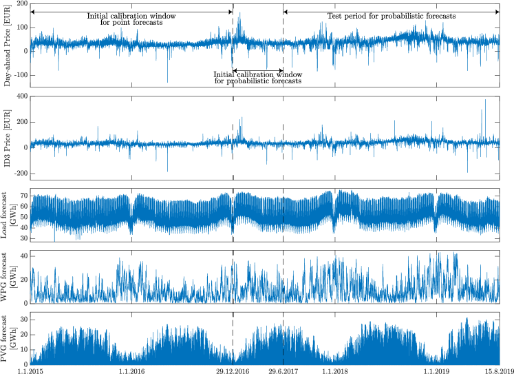
Figure 1: EPEX day-ahead prices (top), EPEX ID3 prices (middle top), day-ahead load prognosis (middle), day-ahead forecasts of wind power generation (middle bottom),day-ahead forecasts of Photovoltaic generation (bottom) from 1.01.2015 to 15.08.2019. The first vertical dashed line marks the end of the 728-day calibration period and the second marks the end of the initial 182-day calibration window for probabilistic forecasts.

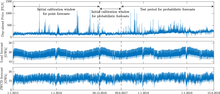
Figure 2: TGE day-ahead prices (top), day-ahead load prognosis (middle), day-ahead forecasts of Generation of Centrally Dispatched Generating Units (JWCD; bottom) from 1.01.2015 to 15.08.2019. The first vertical dashed line marks the end of the 728-day calibration period and the second marks the end of the initial 182-day calibration window for probabilistic forecasts.

In order to test the methodology proposed in this paper, datasets from two European power markets are considered: the German EPEX SPOT and the Polish Power Exchange (TGE).

For the German dataset (EPEX), we consider two different price time series: the day-ahead (DA) hourly electricity prices (top panel in Figure 1) and the corresponding time series linked to the intraday market: the hourly prices of the ID3 index (middle top panel in Figure 1). Since the electricity on the German intraday market is traded continuously, there is no clear definition of the intraday electricity price. The ID3 index is the most common proxy for the above price and is calculated as the volume-weighted average price of all transactions between 180 and 30 minutes before electricity delivery (see Narajewski and Ziel (2020)). In addition to price series, we consider different types of exogenous variables (see Figure 1): day-ahead load forecast (middle panel) as well as day-ahead prediction of wind (middle bottom) and solar power generation (bottom)). Wind generation forecasts consist of the aggregated offshore and onshore generation predictions. All considered series cover the period from 1 January 2015 to 15 August 2019.

The second data series comes from the market operated by the Polish Power Exchange (TGE). The dataset, which also covers the period from 1 January 2015 to 15 August 2019, includes three time series with hourly resolution: day ahead prices for fixing no. 1, day-ahead predictions of system load and day-ahead predictions of the so-called Generation of Centrally Dispatched Generating Units (JWCD); see Figure 2. Note that due to the minimal trading volumes for TGE intraday contracts, contrary to the German data, we do not consider any time series related to the intraday market in Poland.

For both markets, we additionally use two other fundamental indices that affect electricity prices: spot prices of natural gas and the spot price of European carbon emission allowances (EUA - Emission Unit Allowance). Unlike electricity and production forecasts, EUA and Natural Gas are the closing prices and hence are quoted in daily (not hourly) resolution. Additionally, the trading of these commodities takes place from Monday to Friday, and therefore the values for weekend days are substituted by the most recent Friday closing price.

All time series were preprocessed to account for changes to/from the daylight saving time, as in Weron (2006). The missing values (corresponding to changes in the summer time) were substituted by the arithmetic average of the observations from neighboring hours. The doubled values (corresponding to the changes from the summer time) were replaced by their arithmetic mean.

Due to pronounced spikes and seasonality of electricity prices (Janczura et al., 2013), we follow Uniejewski et al. (2018) and apply the Normal-distribution Probability Integral Transform (N-PIT) to all datasets (to time series of prices and exogenous variables). The transformed variable $Y_{d,h}$ for day $d$ and hour $h$ is given by:

$$\tilde{Y}_{d,h}=N^{-1}\left(\hat{F}_{Y_{d,h}}(Y_{d,h})\right),$$ (1)

where $\hat{F}_{Y_{d,h}}(\cdot)$ is the empirical cumulative distribution function of $Y_{d,h}$ in the calibration window, and $N^{-1}$ is an inverse of the normal distribution function.

3 Point Forecasts

In this research, similar to Maciejowska et al. (2019, 2020), we consider a day-ahead forecasts of intraday and day-ahead prices. Since they are obtained at the same time, they are based on identical information sets and can be used for risk management or trading activities that involve taking positions on both markets (see Maciejowska et al. (2019), Janczura and Wójcik (2022)).

3.1 Model for Day-ahead markets

The choice of the benchmark model is motivated by two factors. First, studies on automated variable selection (Uniejewski et al. (2016); Weron and Ziel (2018)) allow us to optimize the structure of the model and include only the most important predictors. Note that in comparison to most common EPF model structures, we additionally include the emission allowance price and the natural gas price because we believe that they may play an important role in the formation of electricity prices. Second, the computational efficiency required to produce probabilistic forecasts is extremely high. Thus, to minimize the computational burden needed to obtain point forecasts, we decide to use simple autoregressive structure with exogenous variables instead of more complex machine learning techniques. We have decided to consider a parsimonious autoregressive structure, inspired by the ARX model of Weron and Misiorek (2008). The model for the transformed day-ahead price on day $d$ and hour $h$ is given by:

$$DA_{d,h}= ~{}\underbrace{\beta_{h,1}DA_{d-1,h}+\beta_{h,2}DA_{d-2,h}+\beta_{h,3}DA_{d-7,h}}_{\scriptsize\mbox{autoregressive effects}}$$

$$+\underbrace{\beta_{h,4}DA_{d-1,min}+\beta_{h,5}DA_{d-1,max}}_{\scriptsize\mbox{non-linear effects}}+\underbrace{\beta_{h,6}DA_{d-1,24}}_{\scriptsize\mbox{midnight price}}$$

$$+\underbrace{\beta_{h,7}L_{d,h}}_{\scriptsize\mbox{load forecast}}+\underbrace{\mathds{1}_{8<h<18}\quad\beta_{h,8}S_{d,h}}_{\scriptsize\mbox{solar gen. forecast}}+\underbrace{\beta_{h,9}W_{d,h}}_{\scriptsize\mbox{wind gen. forecast}}$$

$$+\underbrace{\beta_{h,10}EUA_{d-1}}_{\scriptsize\mbox{emission allowance price}}+\underbrace{\beta_{h,11}NG_{d-1}}_{\scriptsize\mbox{natural gas price}}$$

$$+\underbrace{\sum_{i=1}^{7}\beta_{h,11+i}D_{i}}_{\scriptsize\mbox{weekday dummies}}+\varepsilon_{d,h},$$ (2)

where $DA_{d-1,h}$, $DA_{d-2,h}$, $DA_{d-7,h}$ include information about autoregressive effects and correspond to prices at the same hour of the previous day, two days earlier, and one week earlier. $DA_{d-1,min}$, $DA_{d-1,max}$ and $DA_{d-1,24}$ represent the minimum, maximum, and last known prices of day $d-1$. $L_{d,h}$, $S_{d,h}$ and $W_{d,h}$ refer to the transformed day-ahead load, photovoltaic generation, and wind power generation forecasts for given hour of a day, respectively. Finally, $D_{1},...,D_{7}$ are weekday dummies and $\varepsilon_{d,h}$ is the noise term. Note that solar generation forecasts, $S_{d,h}$, are included only in the models describing German electricity markets (due to Polish data availability issues). Furthermore, due to lack of generation during night and evening hours, the variable is considered in regressions (2)-(3) only for hours 9-17.

3.2 Model for EPEX intraday market

The second model is used to predict the German intraday market price for the next day, computing the forecast on the preceding day $d-1$ (analogously to the DA case). Consequently, intraday and day-ahead prices are forecasted with a very similar methodology: prices for all 24 hours in day $d$ are forecasted simultaneously, using the same pool of information. The model, denoted by $\mathbf{IDA}$ (Intraday Day-Ahead) assumes that the data-generating process of intraday prices could be described by the following equation:

$$ID3_{d,h}= ~{}\underbrace{\beta_{h,1}ID3_{d-1,h}^{*}+\beta_{h,2}ID3_{d-2,h}+\beta_{h,3}ID3_{d-7,h}}_{\scriptsize\mbox{autoregressive effects}}+$$

$$+\underbrace{\beta_{h,4}DA_{d-1,h}}_{\scriptsize\mbox{DA market effect}}+\underbrace{\beta_{h,5}DA_{d-1,24}}_{\scriptsize\mbox{midnight price}}+$$

$$+\underbrace{\beta_{h,6}DA_{d-1,min}+\beta_{h,6}DA_{d-1,max}}_{\scriptsize\mbox{non-linear effects}}+$$

$$+\underbrace{\beta_{h,7}L_{d,h}}_{\scriptsize\mbox{load forecast}}+\underbrace{\mathds{1}_{8<h<18}\quad\beta_{h,9}S_{d,h}}_{\scriptsize\mbox{solar gen. forecast}}+\underbrace{\beta_{h,10}W_{d,h}}_{\scriptsize\mbox{wind gen. forecast}}+$$

$$+\underbrace{\beta_{h,11}EUA_{d-1}}_{\scriptsize\mbox{emission allowance}}+\underbrace{\beta_{h,12}NG_{d-1}}_{\scriptsize\mbox{natural gas}}+$$

$$+\underbrace{\sum_{i=1}^{7}\beta_{h,12+i}D_{i}}_{\scriptsize\mbox{weekday dummies}}+\varepsilon_{d,h},$$ (3)

Note that the model (3) is very similar to the model $\mathbf{DA}$ except that the three autoregressive predictors refer to ID3 prices instead of Day-Ahead and additionally the model includes the Day-Ahead price for the same hour of the previous day. Furthermore, the variable responsible for the price on day $d-1$ is marked with an asterisk, that is $ID3_{d-1,h}^{*}$, because the predictor changes depending on the hour $h$. Due to the fact that forecasting is performed for all hours at the same time, i.e. at 10:00, for later hours the value of the ID3 index for day $d-1$ has not been established yet. Therefore, the value of $ID3_{d-1,h}^{*}$ is the following:

$$ID3_{d-1,h}^{*}=\begin{cases}ID^{\mathrm{partial}}_{d-1,h}&\mbox{for }h>10,\\ ID3_{d-1,h}&\mbox{for }h\leq 10,\end{cases}$$ (4)

where $ID^{\mathrm{partial}}_{d-1,h}$ is the volume-weighted average price of all transactions for a certain product that have occurred up to the time of forecasting. If there were no transactions, $ID^{\mathrm{partial}}_{d-1,h}$ is replaced by the corresponding day-ahead price.

3.3 Forecasting framework

The model weights in Equations 2 and 3, $\boldsymbol{\beta_{h}}$, are estimated by minimizing the Residual Sum of Squares (RSS), independently for each hour in the out-of-sample period (see Section 2). We are considering a rolling calibration window scheme, but rather than arbitrarily choosing a fixed calibration window length, we consider data samples ranging from 56 up to 728 days. By $\hat{P}_{d,h}(\tau)$, we denote the forecast for day $d$ and hour $h$, estimated using the $\tau$-day calibration window. For each day and hour, we obtain 673 different forecasts and, as shown in recent studies (Serafin et al., 2019), the information contained in such a rich panel of forecasts may lead to predictions that statistically outperform any single-window-based forecast. Furthermore, the performance of these predictions is usually more consistent across different data sets (Maciejowska et al., 2020). Point forecasts obtained from the autoregressive models are the basis for all probabilistic models considered in this paper.

4 Probabilistic forecast

In recent years, probabilistic forecasting has gained attention in the EPF literature, as it complements point predictions with additional information about potential trade risk. In this article, quantile regression methods are applied to approximate the distribution of electricity prices. We explore the point forecast described in Section 3 and combine them using two different approaches to predict the quantiles of the next day prices.

4.1 Quantile Regression Averaging

Quantile regression (QR) is a general approach, which allows to represent a quantile of order $\alpha$ of a dependent variable, here $\hat{P}^{\alpha}_{d,h}$, as a linear function of a set of inputs $X_{i,d,h}$:

$$\hat{P}^{\alpha}_{d,h}=w_{0,\alpha}+\sum_{i=1}^{K}w_{i,\alpha}X_{i,d,h}.$$ (5)

The parameters $w_{0,\alpha},...,w_{K,\alpha}$, are estimated by minimizing the so-called pinball score, given by:

$$PS_{\alpha}=\begin{cases}(1-\alpha)(\hat{P}^{\alpha}_{d,h}-P_{d,h})&\text{ for }P_{d,h}<\hat{P}^{\alpha}_{d,h},\\ \alpha(P_{d,h}-\hat{P}^{\alpha}_{d,h})&\text{ for }P_{d,h}\geq\hat{P}^{\alpha}_{d,h}.\end{cases}$$

The estimation process can be carried out separately for 99 percentiles: $\alpha=0.01,...,0.99$ and hence allows us to approximate the whole distribution of $P_{d,h}$.

In recent years, QR has been used successfully as a method of forecast averaging. Nowotarski and Weron (2015) proposed to use multiple point forecasts as input in (5) and showed that such Quantile Regression Averaging (QRA) approach results in more accurate interval forecasts compared to individual models. The idea was next explored and developed by various authors (Maciejowska and Nowotarski (2016), Marcjasz et al. (2019), Serafin et al. (2019), among others). Marcjasz et al. (2019) proposed a modification called the Quantile Regression Machine (QRM), which first applies a simple mean to the average of the point forecasts and then uses the improved prediction as a single input in QR. The above two forecast averaging schemes have been compared by Serafin et al. (2019), who indicate that QRM outperforms QRA, when the averaging is applied to predictions derived from a single model calibrated to windows of different lengths.

In this research, following Serafin et al. (2019), two model specifications are considered. First, in QRA, the point predictions obtained with six different calibration windows, $\tau=56,84,112,714,721,728$, are selected and used directly as explanatory variables in quantile regression.

$$\hat{P}^{\alpha}_{d,h}=w_{0,\alpha}+\sum_{i=1}^{6}w_{i,\alpha}\hat{P}_{d,h}(\tau_{i}).$$ (6)

In the QRM approach, the six point forecasts $\hat{P}_{d,h}(\tau_{i})$ are first averaged with a simple mean to obtain a single prediction $\hat{P}_{d,h}$. Next, $\hat{P}_{d,h}$ is used as an input in the quantile regression:

$$\hat{P}^{\alpha}_{d,h}=w_{0,\alpha}+w_{1,\alpha}\hat{P}_{d,h}.$$ (7)

The visualizations of the QRA and QRM methods are depicted in the first two blocks of Figure 3.

It should be noticed here that in both methods, only six pre-selected point forecasts are used. This model specification is inspired by Hubicka et al. (2019) and Marcjasz et al. (2018), who demonstrated that combining three short and three long windows results in the largest gains in forecast accuracy. Moreover, Serafin et al. (2019) showed that the inclusion of a larger set of point predictions in the QR can lead to a decrease in the accuracy of the prediction. There are two major reasons for such decrease: (i) when the number of inputs increases parameters are estimated with a larger error, (ii) individual point forecasts are highly correlated so new inputs bring only little or no additional information to the model.

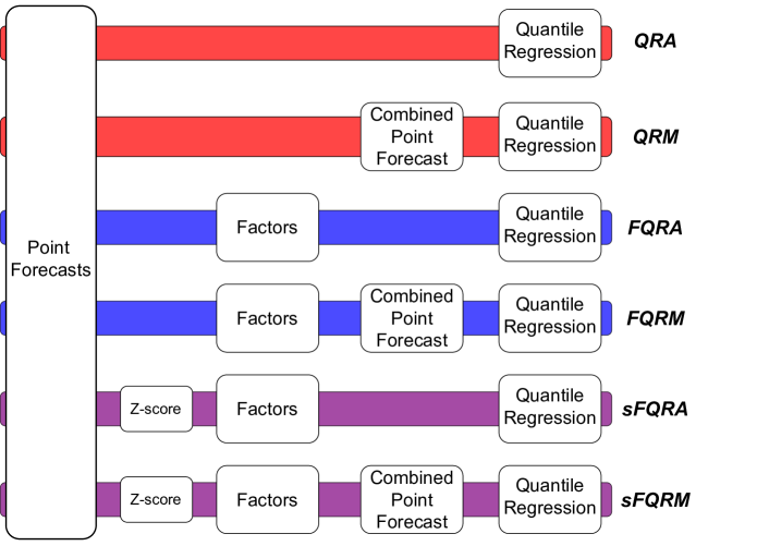
Figure 3: The flowchart illustrating the subsequent steps of each forecasting model.

4.2 Factor Quantile Regression Averaging

Although in QRA and QRM methods we only utilize six point forecasts, all predictions from calibration windows ranging from 56 up to 728 days are the base for the next group of probabilistic models. In order to explore the whole panel of 673 point forecasts, which are strongly correlated and therefore should not be used jointly in a regression model, similar to to Maciejowska et al. (2016) and Uniejewski and Maciejowska (2022), we propose to use the Principal Components analysis (PCA). PCA allows to represent a large number of variables with a few principle components, called factors, which are orthogonal by assumption and therefore solve the mentioned colinearity problem. Being one of the most popular methods of dimension reduction technique (Velliangiri et al. (2019), He et al. (2021), Guo et al. (2022)), PCA has been shown to be helpful in the construction of probabilistic forecasts. Maciejowska et al. (2016) proposed to apply quantile regression to the first, most prominent factor and denote it by Factor Quantile Regression Averaging (FQRA). On the basis of empirical studies, the authors conclude that FQRA outperforms standard QRA. In that work, PCA is applied to a relatively small panel of predictions stemming from 32 different models/model specifications.

Here, following Maciejowska et al. (2020) and Uniejewski and Maciejowska (2022), we explore a slightly modified approach. First, probabilistic forecasts are computed jointly for all hours of a day with a single model rather than with a separate model for each hour. Hence, the electricity prices and their predictions are treated as time series, with a time index $t=24(d-1)+h$. In order to estimate the weights in the QRA, last 182 days are used. Since we extract factors for both the past and the current data, the analyzed window is extended by additional $24$ forecasts of hourly prices from the forecast day, $d_{f}$. Let us denote by $\hat{P}_{t}(\tau)$ the prediction of the variable $P_{t}$ based on a calibration window of length $\tau$. The data set $\hat{P}=\{\hat{P}_{t}(\tau)\}$ constitutes a panel, with the first dimension representing time and the second dimension describing the size of a calibration window.

All PCA-based models rely on common factors extracted from the panel of point forecasts $\hat{P}$. Factors are estimated as scaled eigenvectors of a matrix $\hat{P}\hat{P}^{\prime}$ (see Stock and Watson (2002) for more details). Next, they are used twofold in the process of obtaining price percentile forecasts. They are either utilized to obtain first the point forecast (as in Maciejowska et al. (2020)) which is then taken as the input for the quantile regression or are directly used as the regressors for the quantile prediction estimation. We denote the first approach as FQRM/sFQRM and the second as FQRA / sFQRA, which correspond to the QRM and QRA methods discussed in Section 4.1 (see Figure 3). The detailed regression equations for these methods are presented below. In FQRA/sFQRA models, a quantile regression is used as a link between the factors summarizing point forecasts and the quantile of electricity price

$$P^{\alpha}_{t}=w_{0,\alpha}+\sum_{k=1}^{K}w_{k,\alpha}F_{t,k}$$ (8)

where $F_{t,k}$ is the value of a $k$-th factor at the time $t$, with $k=1,...,K$. Similarly to the QRM approach, in the FQRM/sFQRM methods, the point forecast is first calculated using a linear regression.

$$P_{t}=\alpha+\sum_{k=1}^{K}\beta_{k}F_{t,k}+e_{t}.$$ (9)

Next, the predictions $\hat{P}_{t}$ obtained with the above model are used in a quantile regression

$$\hat{P}^{\alpha}_{t}=w_{0,\alpha}+w_{1,\alpha}\hat{P}_{t},$$ (10)

In both cases, regressions (8) and (9), Bayesian Information Criterion (BIC) is used to select the optimal number of factors, $K$. A similar procedure has been adopted by Maciejowska et al. (2020) and Uniejewski and Weron (2021).

Finally, we consider two specifications of FQRA and FQRM approaches, which depend on a standardization of the input data. In FQRA/FQRM methods, factors are estimated directly from the panel $\hat{P}$. Whereas in sFQRA and sFQRM approaches, similar to Maciejowska et al. (2020), the data is first standardized, according to the formula

$$\hat{p}_{t}(\tau)=\frac{\hat{P}_{t}(\tau)-\hat{\mu}_{t}}{\hat{\sigma}_{t}},$$

where $\hat{\mu}_{t}$ is the mean and $\hat{\sigma}_{t}$ is the standard deviation of forecasts $\hat{P}_{t}(\tau)$ across different window sizes, $\tau$. The standardization step is denoted as Z-Score in Figure 3. Next, the panel $\hat{p}=\{\hat{p}_{t}(\tau)\}$ is used to estimate factors, $F_{t}$. Whenever the standardization is used, it is also applied to the predicted variable

$$p_{t}=\frac{P_{t}-\hat{\mu}_{t}}{\hat{\sigma}_{t}}.$$ (11)

It should be noticed that $\hat{p}$ and $p$ have different units than $\hat{P}$ and $P$. Therefore, once the predictions of quantiles $\hat{p}^{\alpha}_{t}$ are calculated with (8) or (10), they are transformed back into the original units

$$\hat{P}^{\alpha}_{t}=\hat{p}^{\alpha}_{t}*\hat{\sigma}_{t}+\hat{\mu}_{t}.$$ (12)

Empirical analysis indicates that the standardization has a significant impact on the performance of the proposed averaging schemes.

Tu sum up, Factor Quantile Regression averaging method consists of the following steps (depicted on Figure 3):

1. The panel $\hat{P}=\{\hat{P}_{t}(\tau)\}$ is constructed from a set of point forecasts $\hat{P}_{d,h}(\tau)$. In sFQRA and sFQRM approaches, the data is further standardized and denoted by $\hat{p}$.

2. $K$ factors summarizing the information in the panel $\hat{P}$ or $\hat{p}$ are estimated with PCA method

3. Estimated factors, $F_{t,k}$, are used to compute probabilistic forecasts with quantile regression using equations (8) or (9)-(10)

4. In sFQRA and sFQRM methods, the predictions are transformed into the original units with (12).

5 Evaluation of forecasts

In order to evaluate probabilistic forecasts, we consider two types of approaches. First, the predictions are assessed with statistical measures such as an empirical coverage level, which show how accurate are the predictions of the distribution quantiles. The statistical significance of the results is verified with a Christoffersen test (Christoffersen (1998)). Next, the obtained forecasts are used as an input to the trading strategy. The strategy allows for the assessment of the practical utility of obtained predictions. Their performance is compared in context of economic measures such as an average profit, a profit per 1 MWh traded and the average traded volume.

5.1 Statistical evaluation

Model	$EPEX_{DA}$			$EPEX_{IDA}$			$POL$
	80 %	90 %	98 %	80 %	90 %	98 %	80 %	90 %	98 %
QRA	75.70	85.53	95.05	76.39	86.24	95.45	75.40	85.56	94.57
QRM	76.59	86.56	95.96	77.09	86.91	96.02	77.14	87.29	95.68
FQRA	78.14	88.35	96.66	78.25	88.34	97.11	81.40	90.76	97.91
FQRM	77.78	88.08	96.47	78.91	88.13	96.90	81.53	90.75	97.94
sFQRA	80.41	90.33	98.08	80.89	90.42	98.01	79.03	89.45	97.90
sFQRM	80.31	90.27	97.93	80.25	90.08	97.87	79.49	89.51	97.71

Table 1: The Empirical Coverage of prediction interval of $\alpha=80\%,90\%,\text{and }98\%$ from all considered probabilistic forecasting methods. The results are divided into three sub-tables, for EPEX SPOT, EPEX ID3 and Polish TGE (consecutively from left to right). The value closest to the nominal coverage in each column is bolded.

Model	$EPEX_{DA}$			$EPEX_{IDA}$			$POL$
	80 %	90 %	98 %	80 %	90 %	98 %	80 %	90 %	98 %
QRA	4.30	4.47	2.95	3.61	3.76	2.55	4.83	4.61	3.43
QRM	3.41	3.44	2.04	2.91	3.09	1.98	3.84	3.22	2.32
FQRA	6.67	4.29	1.88	5.73	3.84	1.27	3.14	2.39	0.91
FQRM	6.74	4.47	1.91	5.64	4.16	1.58	3.50	2.30	0.81
sFQRA	1.98	1.45	0.52	1.71	1.24	0.48	1.93	1.20	0.57
sFQRM	2.20	1.55	0.63	1.86	1.44	0.48	1.76	1.20	0.69

Table 2: The Mean Absolute Deviation of prediction interval of $\alpha=80\%,90\%,\text{and }98\%$ from all considered probabilistic forecasting methods. The results are divided into three sub-tables, for EPEX SPOT, EPEX ID3 and Polish TGE (consecutively from left to right). The value closest to zero in each column is bolded.

In this article, quantile forecasts are used for building prediction interval (PI). A PI of a nominal level $\alpha$ is constructed as $PI^{\alpha}_{d,h}=[\hat{L}^{\alpha}_{d,h},\hat{U}^{\alpha}_{d,h}]$, where $\hat{L}^{\alpha}_{d,h}=\hat{P}^{\frac{1-\alpha}{2}}_{d,h}$ and $\hat{U}^{\alpha}_{d,h}=\hat{P}^{\frac{1+\alpha}{2}}_{d,h}$ are the forecasted quantiles of electricity prices. The competing forecast averaging schemes are first compared on the basis of their empirical coverage (Chatfield (1993)). For each day and hour of the 778-day out-of-sample period we calculate the ’hits’ of the prediction intervals:

$$I^{\alpha}_{d,h}=\begin{cases}1&\text{if }P_{d,h}\in[\hat{L}^{\alpha}_{d,h},\hat{U}^{\alpha}_{d,h}]\\ 0&\text{if }P_{d,h}\not\in[\hat{L}^{\alpha}_{d,h},\hat{U}^{\alpha}_{d,h}].\end{cases}$$ (13)

Next, the average number of ’hits’ is calculated, which represents an empirical coverage level. For a given hour $h$, it is computer as

$$Cov^{\alpha}_{h}=\frac{1}{778}\sum_{d}I^{\alpha}_{d,h}$$ (14)

and the average daily coverage becomes

$$Cov_{\alpha}=\frac{1}{24}\sum_{h}Cov^{\alpha}_{h}.$$ (15)

The distance of an empirical coverage from its nominal level, $\alpha$, is evaluated twofold. First, a Mean Absolute Deviation of $Cov_{\alpha}$ is calculated as

$$MAD_{\alpha}=\frac{1}{24}\sum_{h}|Cov^{\alpha}_{h}-\alpha|.$$ (16)

It helps to assess the behavior of the methods throughout the day. Next, the hypothesis $H_{0}:Cov^{\alpha}_{h}=\alpha$ is tested with the Christoffersen’s test (Christoffersen (1998)) for each hour separately. The test takes into account not only the unconditional coverage of prediction intervals ($Cov^{\alpha}_{h}$) but also the independence of the quantile level exceedances in consecutive time periods. This particular property of probabilistic forecasts is often overlooked in the literature, since most of the studies focus solely on the unconditional coverage of prediction intervals. Christoffersen’s test can be seen as an extension of a popular Kupiec test (Kupiec (1995)).

5.1.1 Results

We consider three levels of coverage: $\alpha=80\%,90\%,98\%$ to compare the prediction accuracy of the proposed methods. In Table 1, we report the empirical coverage, $Cov_{\alpha}$ for three markets and six methods analyzed in this study. It should be noted that for accurate $PI$ predictions, the empirical coverage will be close to its nominal level. Next, the daily profiles of $Cov^{\alpha}_{h}$ are depicted in Figure 4. We show only the results for the 90% nominal coverage level as the shapes for 80% and 98% coverage values are very similar and therefore do not change the conclusions. Finally, Table 2 presents $MAD_{\alpha}$, which summarizes the behavior of the empirical coverage level across all hours of the day. Similarly to other dispersion measures, lower values of $MAD_{\alpha}$ indicate more accurate forecasts. The presented results lead to the following conclusions:

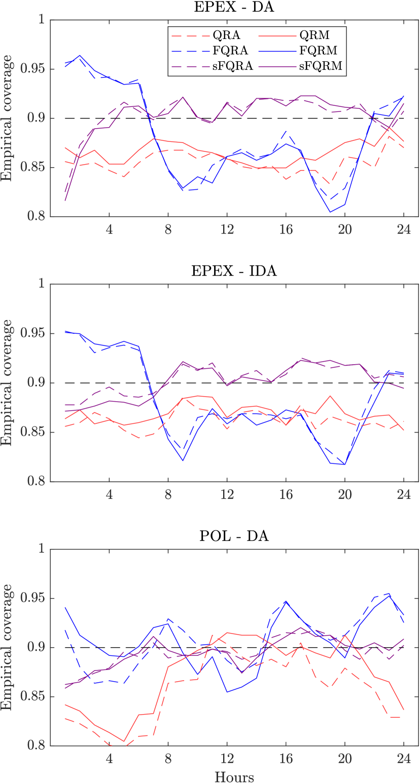
Figure 4: The averaged daily profile of the empirical coverage for 90 % prediction intervals for EPEX SPOT (top), EPEX ID3 (middle) and Polish TGE (bottom) markets. The QRA-type models and indicated with dashed lines, while the QRM-type models and depicted with solid lines.

• When empirical coverage is considered (Table 1), sFQRA and sFQRM methods clearly outperform their competitors. In eight out of nine cases, they provide predictions with the empirical coverage being the closest to the nominal level. Additionally, it could be noticed that QRA/QRM benchmarks provide $PI$’s which are on average too narrow and hence are characterized with empirical coverage much below the nominal level. The results of FQRA/FQRM methods fall between the benchmark and the standardized approaches,

• The initial conclusions are confirmed by the daily profiles of empirical coverage presented in Figure 4. It could be seen that for the sFQRA/sFQRM methods, the empirical coverage oscillates around 90%, with the only exception for early night hours: 1-2, when they fall short of the nominal level. Unlike standardized factor approaches, FQRA/FQRM methods provide either visibly too wide (hours 1-6) or too narrow (hours 8-21) prediction intervals. Therefore, the results indicate that standardization plays an important role in the construction of probabilistic forecasts and helps to model price volatility.

• Forecasts from QRA and QRM models exhibit a constantly lower coverage for all datasets and all values of the nominal coverage. This is also true for the daily profiles of the coverage (see Figure 4). For the EPEX dataset, for each hour of the day, the empirical coverage of forecasts is lower than the nominal one. For the Polish market, this is true for most hours of the day.

• Analysis of $MAD$ shows that sFQRA provides prediction intervals, which deviate the least from the nominal level. The results for sFQRM are only slightly worse and both exhibit a much lower $MAD$ than FQRA/FQRM and QRA/QRM methods.

Table 3 shows the number of hours (out of 24), for which the null of the Christoffersen test was not rejected. This indicates that the empirical coverage is close enough to the nominal level and that quantile exceedances are independent. Based on the results, we can conclude that:

• The forecasts from the sFQRA and sFQRM models pass the Christoffersen test for the largest amount of hours for each nominal coverage value and all datasets. The difference is especially profound for the 98% prediction intervals.

• The performance of the FQRA/FQRM and QRA/QRM models differs across the nominal coverage levels. The latter models pass the Christoffersen test for a slightly higher number of hours for the 80% and 90% levels. However, for the 98% nominal coverage, forecasts from FQRA and FQRM models outperform both literature benchmarks by a large margin.

To sum up, statistical measures show that sFQRA and sFQRM forecast averaging methods outperform their FQRA/FQRM and QRA/QRM counterparts. They help construct PIs for which empirical coverage deviates the least from its nominal level. It should be noted here that, at the same time, FQRA/FQRM methods provide outcomes that, despite their increased computational complexity, are not much better than those of QRA/QRM approaches. It underlines that standardization plays a very important role in estimating the averaging weights.

	Coverage 80%			Coverage 90%			Coverage 98%
Model	$EPEX_{DA}$	$EPEX_{IDA}$	$POL$	$EPEX_{DA}$	$EPEX_{IDA}$	$POL$	$EPEX_{DA}$	$EPEX_{IDA}$	$POL$
QRA	0	2	3	0	0	1	0	0	1
QRM	0	2	4	1	2	5	0	1	4
FQRA	0	0	0	1	1	1	4	11	4
FQRM	0	0	0	0	1	1	4	9	8
sFQRA	9	17	4	14	21	12	20	23	19
sFQRM	10	17	3	12	20	17	17	22	19

Table 3: Results of the conditional Christoffersen test. The table shows the number of hours of the day (out of 24) for which the null hypothesis of the Christoffersen test is not rejected at the 5% significance levels. The results are divided into three sub-tables for prediction interval of $\alpha=80\%,90\%,\text{and }98\%$ (consecutively from left to right).

5.2 Economic evaluation

The vast majority of articles focus on the evaluation of forecasts and the comparison of predictive models based on statistical measures. Although popular, this approach possesses a number of drawbacks, one of the most important being the choice of the evaluation measure. As Kolassa (2020) argues, the term ’best forecast’ depends strongly on the choice of the evaluation measure. Therefore, in order to properly assess the forecasts in the objective manner, an auxiliary measure should be introduced. Evaluating forecasts with the use of economic measure, such as profit, not only provides an universal approach applicable to any forecast (generated by minimizing any given loss function), but also gives the valuable information about the real-life utility of generated forecasts.

5.2.1 Trading strategy

Although only a few articles in the EPF literature consider economic measures for the evaluation of forecasts and the classification of predictive models, the topic has recently started gaining the attention of researchers in the field of EPF Maciejowska et al. (2022). The base for the economic assessment of forecasts is the trading strategy that mimics the actual behavior of market participants such as speculators, energy generators or energy consumers. Among the strategies considered in the literature, numerous involve trading electricity in the day-ahead market or continuous intraday markets (Maciejowska et al., 2021; Uniejewski and Weron, 2021; Serafin et al., 2022). Several authors consider a one-sided approach, taking the perspective of the supplier or consumer (Zareipour et al., 2010; Doostmohammadi et al., 2017; Janczura and Wójcik, 2022), while others propose a trading strategy that involves an electricity storage system (Kath and Ziel, 2018; Uniejewski and Weron, 2021; Uniejewski, 2022).

5.2.2 Quantile-based trading strategies

In this article, to evaluate the economic value of forecasts, we consider a trading strategy proposed in Uniejewski (2022). The idea of the strategy is to sell at high prices and buy at low prices, based on the levels determined by the forecasted quantiles. Let us assume that the trader has access to an available 2 MW energy storage space and aims to sell (discharge battery) and buy (charge battery) 1 MWh of electricity each day. Each day, he/she has to decide about when (at which hours) and at what price to submit the bid and offer on the market. Using the proposed strategy, we will show how probabilistic forecasts can be applied to support the decision-making and energy trading process.

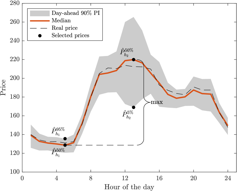
Figure 5: An example of the quantile-based trading strategy of Uniejewski (2022) for Polish market on 06.07.2017. Red line indicates the median forecast ($\hat{P}^{50\%}_{d,h}$) and the dashed black line presents the real price. The grey space depicts the day-ahead forecast of the 90% prediction interval, while dots at the PI limits represent the offer $\hat{P}^{5\%}_{d,h_{2}}$ and bid $\hat{P}^{95\%}_{d,h_{1}}$ prices.

Note that when dealing with strategies based on an energy storage system, we have to take into account that no battery has perfect efficiency. Therefore, let us assume that both charge and discharge processes have an efficiency of ca. 90%. This means that when 1 MW is discharged, we will only sell 0.9 MWh and, respectively, we need to buy $\frac{1}{0.9}$ MWh to fully recharge the battery.

First, the trader decides when to place bid and offer based on the median forecasts, and then in the second step, the bid and offer levels are establishes using the quantile forecasts. Even though the trader aims to both sell and buy 1 MWh per day and consequently stay with the same amount of energy in the storage system at the end of each day, depending on the market prices, the submitted bids and offers can be both accepted or rejected. Therefore, there are three battery states that may occur at the beginning of each day. Depending on which state the battery is on day $d$, the trader will take different actions:

• If the battery is empty ($B_{d}=0$) and there is no more energy to sell at the beginning of day $d$ the trader will submit an additional price-taker bid to close the position from the previous day. In this scenario, the trader will submit two bids to buy energy (1 MWh per transaction) and one offer to sell. He will then need to select three hours at which the transitions will take place, having in mind that the unlimited (price-taker) bid has to be submitted on the earlier hour than the offer. Taking into account the energy storage efficiency to select the optimal hours to submit bids and offer, we have to solve the following problem:

  $$\max_{h_{1},h_{2},h^{*}}\left(0.9~{}\hat{P}^{50\%}_{d,h_{2}}-\frac{1}{0.9}\hat{P}^{50\%}_{d,h_{1}}-\frac{1}{0.9}\hat{P}^{50\%}_{d,h^{*}}\right),$$ (17)

  subject to: $h^{*}<h_{2}$,

  where $h_{1}$ and $h_{2}$ are the hours for which we submit the ’limited’ bid and offer, respectively, while $h^{*}$ refers to the hour for which we perform the price-taker buy (submit unlimited bid).

• If the battery is half full ($B_{d}=1$) the battery can be charged and discharged and no additional actions are required. In this scenario, the trader selects two hours – one at which he will submit the bid to buy that is with the lowest price on a given day indicated by $h_{1}$ and one with the highest price denoted by $h_{2}$ at which the energy will be offered to sell.

• If the battery is full ($B_{d}=2$) and it is impossible to charge the battery at the beginning of day $d$ the trader will submit an additional price-taker offer to close the position from the previous day. In such a scenario, the trader will submit one bid to buy energy and two offers to sell (1 MWh per transaction). He will then need to select three hours at which the transitions will take place, having in mind that the unlimited (price-taker) offer has to be submitted on the earlier hour than the bid. To select the optimal hours to submit bid and offers, we have to solve the following problem:

  $$\max_{h_{1},h_{2},h^{*}}\left(0.9~{}\hat{P}^{50\%}_{d,h_{2}}-\frac{1}{0.9}\hat{P}^{50\%}_{d,h_{1}}+0.9\hat{P}^{50\%}_{d,h^{*}}\right),$$ (18)

  subject to: $h^{*}<h_{1}$.

  where $h_{1}$ and $h_{2}$ are the hours for which we submit the bid and the ’limited’ offer, respectively, while $h^{*}$ refers to the hour for which we perform the price-taker sale (submit unlimited offer).

Having the optimal hours selected, the trader needs to make a decision about the bid and offer prices. First, the trader chooses the prediction interval level $\alpha$: PI $=[\hat{L}_{d,h}^{\alpha}$, $\hat{U}_{d,h}^{\alpha}]$. The bid price is then set as the upper limit of the PI and equals $\hat{U}_{d,h_{1}}^{\alpha}=\hat{P}_{d,h_{1}}^{\frac{1+\alpha}{2}}$, while the offer price is set as the lower bound of the PI and equals $\hat{L}_{d,h_{1}}^{\alpha}=\hat{P}_{d,h_{1}}^{\frac{1-\alpha}{2}}$. If the additional price-taker transaction is required, the bid or offer is submitted for hour $h^{*}$ at the maximum or minimum market price.

Finally, we calculate the basic profit obtained with the procedure for day $d$ according to Table 4. That is, if both the bid and the offer are accepted, the trader buys $\frac{1}{0.9}$ MWh at hour $h_{1}$ and sells 0.9 MWh at hour $h_{2}$ at the market price $P_{d,h_{1}}$ and $P_{d,h_{2}}$, respectively. On the contrary, if both bid and offer were rejected, the daily profit is equal to 0. If only a bid or only an offer is accepted, the daily gain or daily loss is offset by the change in battery status.

Furthermore, a profit from closing a previous day position is calculated. If on day $d-1$ only the offer was accepted (Case 3, Table 4) then on day $d$ the battery is empty. Hence the trader additionally buys $\frac{1}{0.9}$ MWh at hour $h^{*}$, so the daily profit decreases by $\frac{1}{0.9}P_{d,h^{*}}$ and the battery is charged with 1MW. On the contrary, if on day $d-1$ only the bid is accepted (Case 2, Table 4) then the battery is full at the beginning of day $d$ ($B_{d}=2$). Therefore the trader additionally sells $0.9$ MWh at hour $h^{*}$, so the daily profit increases by $0.9P_{d,h^{*}}$ and the battery is discharged by 1MW. The final profit on a day $d$ is the sum of the basic profit (Table 4) and an additional profit from closing the position.

Case 1	Case 2	Case 3	Case 4
Conditions
$P_{h_{1}}\leq\hat{P}^{1-\alpha}_{d,h_{1}}$	$P_{h_{1}}\leq\hat{P}^{1-\alpha}_{d,h_{1}}$	$P_{h_{1}}>\hat{P}^{1-\alpha}_{d,h_{1}}$	$P_{h_{1}}>\hat{P}^{1-\alpha}_{d,h_{1}}$
$P_{h_{2}}\geq\hat{P}^{\alpha}_{d,h_{2}}$	$P_{h_{2}}<\hat{P}^{\alpha}_{d,h_{2}}$	$P_{h_{2}}\geq\hat{P}^{\alpha}_{d,h_{2}}$	$P_{h_{2}}<\hat{P}^{\alpha}_{d,h_{2}}$
Traded volume
2 MWh	1 MWh	1 MWh	0 MWh
Profit from trade
$0.9~{}P_{d,h_{2}}-\frac{1}{0.9}P_{d,h_{1}}$	$-\frac{1}{0.9}P_{d,h_{1}}$	$0.9~{}P_{d,h_{2}}$	0
Battery state
$B_{d+1}=1$	$B_{d+1}=2$	$B_{d+1}=0$	$B_{d+1}=1$

Table 4: Calculation of a basic profit and a battery state: Case 1 – both bid and offer are accepted, Cases 2 and 3 – only one transaction (bid or offer, respectively) is accepted, Case 4 – rejection of both trades.

5.2.3 Unlimited-bids benchmark

The profits made with strategies using probabilistic forecasts are compared with a simple unlimited bid strategy. Here, the trader selects the moment of transaction by exploring the point forecasts and chooses the hours corresponding to the lowest ($h_{1}$) and highest ($h_{2}$) predicted prices. Then the price-taker offer is submitted to sell at hour $h_{2}$ and the price-taker bid is submitted to buy at hour $h_{1}$. The daily profit that takes into account the efficiency of the battery is calculated as $0.9P_{d,h_{2}}-\frac{1}{0.9}P_{d,h_{1}}$.

5.2.4 Results

In this paper, similarly to Uniejewski (2022), we compare quantile-based trading strategies for different prediction interval levels ranging from 50% to 98% and different forecasting models. Since the trading volume can differ, based on the choice of model and prediction interval level, we report the relative profits defined as an average gain obtained per single 1 MWh transaction, as well as the average traded volume.

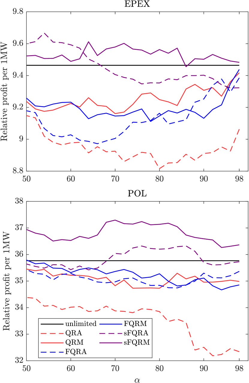
Figure 6: The profits per 1 MWh traded for EPEX SPOT (in Euro; top panel) and Polish (in PLN; bottom panel). The red lines refer to the profits obtained with QRA (dashed line) or QRM (solid line), the blue ones represent FQRA (dashed) and FRQM (solid) and the purple ones depict sFQRA (dashed) and sFQRM (solid). The results of the unlimited bid strategy are plotted with solid black line.

In Figure 6, we present the relative profit per 1 MWh traded. The values are calculated as the average gain achieved by the trader using the chosen strategy. The results do not take into account any financial costs (such as the transaction cost) apart from the loss due to a limited load and discharge efficiency. The results lead to the following conclusions:

• The highest average relative profits are obtained with quantile-based trading strategies using the probabilistic forecast from the sFQRM model. The newly proposed model, in terms of economic value, outperforms all competitors for all considered PI’s levels for Polish market and majority of PI’s for EPEX SPOT.

• The second best forecasting model, in terms of economic value, is another newly proposed model – sFQRA. For EPEX SPOT, it yields the highest individual relative profit across all models, obtained for the 54% prediction interval.

• For all three classes of models, the QRM-based variant on average outperforms the QRA-based variant.

• The unlimited bids strategy performs very well and only sFQRA and sFQRM forecasts can outperform it. Moreover, as the PI’s level grows to 100%, the results for all strategies converge to the unlimited-bid benchmark.

• The sFQRM-based strategy yields the highest profit for the PI’s level between 65-85% for the EPEX SPOT and 68-82% for the Polish market.

• For both datasets, the strategies based on energy storage systems allow to obtain reasonable high profits up to 10 Euro per each 1 MWh traded. For the EPEX SPOT, the highest possible relative profit is 9.67 Euro and for Polish market it is 37.30 PLN (around 8.25 Euro).

Table 5: Total profit, relative profit and traded volume relative to unlimited-bids benchmark for EPEX SPOT (top table) and Polish TGE (bottom table) obtained using a range of quantile-based strategies and all considered probabilistic forecasting models.

EPEX
	Total profit %				Profit per 1 MWh %				Volume %
$\alpha$	50	80	90	98	50	80	90	98	50	80	90	98
QRA	89.09	90.76	93.06	95.76	96.67	93.15	94.15	95.76	92.16	97.43	98.84	100.00
QRM	93.59	96.22	97.84	99.38	97.61	97.73	98.34	99.50	95.89	98.46	99.49	99.87
FQRA	93.00	96.32	97.51	99.17	96.99	96.82	97.77	99.17	95.89	99.49	99.74	100.00
FQRM	92.42	95.65	95.87	99.72	97.83	96.64	96.49	99.72	94.47	98.97	99.36	100.00
sFQRA	97.13	98.57	99.34	98.51	101.43	98.83	99.34	98.51	95.76	99.74	100.00	100.00
sFQRM	95.71	100.59	100.40	100.20	100.62	101.04	100.40	100.20	95.12	99.55	100.00	100.00

POL
	Total profit %				Profit per 1 MWh%				Volume %
$\alpha$	50	80	90	98	50	80	90	98	50	80	90	98
QRA	86.12	90.63	89.60	90.31	96.13	94.64	90.88	90.42	89.59	95.76	98.59	99.87
QRM	91.09	95.73	97.61	97.76	99.12	97.10	97.74	97.82	91.90	98.59	99.87	99.94
FQRA	94.16	96.40	98.56	98.88	99.07	97.41	98.69	98.88	95.05	98.97	99.87	100.00
FQRM	92.87	96.72	97.92	97.45	100.07	98.62	98.17	97.45	92.80	98.07	99.74	100.00
sFQRA	92.99	99.91	99.81	99.89	99.65	101.21	99.81	99.89	93.32	98.71	100.00	100.00
sFQRM	95.32	102.23	102.17	101.67	103.29	103.83	102.31	101.67	92.29	98.46	99.87	100.00

In Table 5, we show the total profit, the relative profit and the traded volume for the whole 778-day out-of-sample period. The values are expressed relative to the outcomes of unlimited-bids strategy. This means that values below/above 100% represent results, respectively, lower or higher than the benchmark. For readability, we present only the results for four selected PI’s levels (50%, 80%, 90% and 98%). The outcomes lead to the following conclusions:

• When total profits are considered, the highest results are obtained with 80% PI for sFQRM, 80% or 90% PI for sFQRA and 98% for the remaining trading strategies. The small values associated with low levels of PIs can be explained by the moderate amounts of traded volumes. For example, for 50% PI only 92-95% of potential volumes are traded on the EPEX market. These values drop even further to 89-92% on the Polish market.

• For both datasets, the highest total profits are obtained with a quantile-based strategy using the sFQRM forecast. sFQRM is also the only strategy that allows one to achieve higher profits than the unlimited bids benchmark.

• The profits pre 1 MWh obtained with the sFQRM strategy are up to 1.04% (for EPEX SPOT) and 3.83% (for the Polish market) higher than the results of the unlimited-bids benchmark. In both markets, the highest profits are earned for 80% PIs. This confirms previous findings that the sFQRM approach yields the largest revenues for PI’s levels between 70-80%.

• The unlimited bids strategy trades 2 MW of energy everyday, thus all other strategies cannot have a volume not larger than the benchmark. However, due to the additional price-taker transaction, the total traded volumes for quantile-based strategies are not less than 90% even for 50% PI.

• The optimal results for sFQRM strategy are associated with the trading volumes of 99.55% and 98.46% on the EPEX and Polish markets, respectively. Hence, this strategy allows to trade almost all the time except from periods with the lowest profits.

6 Conclusions

This paper presents a novel approach to constructing probabilistic forecasts that combines both quantile regression averaging and principal component analysis. It extends the earlier work of Maciejowska et al. (2020) that used a PCA forecast averaging scheme to construct point predictions. To assess the precision of the presented methods, factor-based models are applied to predict the distribution of spot electricity prices in three European markets. Their performance is evaluated on an out-of-sample period of more than 2 years. Similarly to Marcjasz et al. (2018) and Hubicka et al. (2019), the point predictions used for the forecast averaging are based on a single ARX model calibrated to windows of different sizes. The final results are evaluated with statistical (empirical coverage and Christoffersen test) and economic measures.

The performance of the proposed averaging schemes is compared with two QRA and QRM methods, which are well established in the literature. The results indicate that factor-based methods, sFQRA and sFQRA in particular, provide predictions that are not only more accurate than benchmarks but also statistically reliable. They have an empirical coverage close to the nominal level and pass the Christoffersen test for majority of hours and markets. Moreover, we compare two specifications of factor models that depend on the data standardization. Unlike in other PCA applications, we normalize the data in the cross-sectional dimension rather than the time dimension. Hence, we take into account both the level and the variability of the predictions across different window sizes. The results indicate that standardization has a huge impact on performance and leads to a significant improvement of forecast accuracy.

Finally, the prediction methods are evaluated with economic measures. We propose an experiment that resembles a decision problem of an energy storage utility. We demonstrate how probabilistic forecasts can be used to build a trading strategy. The outcomes show that more accurate prediction intervals of spot prices result in higher profits, both in absolute terms and per 1 MWh of trade. The greatest gains are obtained for the newly proposed sFQRM method, which outperforms other approaches for almost all levels of PIs and two analyzed markets.

Combining Quantile Regression with dimension reduction techniques, such as PCA, allows to analyze large panels of point predictions and utilize them for probabilistic forecasting. We believe that this research can be further extended as in Uniejewski and Maciejowska (2022), and applied to different commodity markets.

References

- Bunn et al. (2016) Bunn, D., Andresen, A., Chen, D., Westgaard, S., 2016. Analysis and forecasting of electricity price risks with quantile factor models. Energy Journal 37, 101–122.
- Bunn et al. (2018) Bunn, D., Gianfreda, A., Kermer, S., 2018. A trading-based evaluation of density forecasts in a real-time electricity market. Energies 11, 2658.
- Chatfield (1993) Chatfield, C., 1993. Calculating interval forecasts. Journal of Business & Economic Statistics 11, 121–135.
- Christoffersen (1998) Christoffersen, P., 1998. Evaluating interval forecasts. International Economic Review 39, 841–862.
- Churchill et al. (2022) Churchill, S.A., Inekwe, J., Ivanovski, K., Smyth, R., 2022. Human capital and energy consumption: Six centuries of evidence from the united kingdom. Energy Economics , 106465.
- Doostmohammadi et al. (2017) Doostmohammadi, A., Amjady, N., Zareipour, H., 2017. Day-ahead financial loss/gain modeling and prediction for a generation company. IEEE Transactions on Power Systems 32, 3360–3372.
- Guo et al. (2022) Guo, Y., He, F., Liang, C., Ma, F., 2022. Oil price volatility predictability: New evidence from a scaled pca approach. Energy Economics 105, 105714.
- He et al. (2021) He, M., Zhang, Y., Wen, D., Wang, Y., 2021. Forecasting crude oil prices: A scaled pca approach. Energy Economics 97, 105189.
- Hong et al. (2020) Hong, T., Pinson, P., Wang, Y., Weron, R., Yang, D., Zareipour, H., 2020. Energy forecasting: A review and outlook. IEEE Open Access Journal of Power and Energy 7, 376–388.
- Hubicka et al. (2019) Hubicka, K., Marcjasz, G., Weron, R., 2019. A note on averaging day-ahead electricity price forecasts across calibration windows. IEEE Transactions on Sustainable Energy 10, 321–323.
- Huntington and Liddle (2022) Huntington, H., Liddle, B., 2022. How energy prices shape oecd economic growth: Panel evidence from multiple decades. Energy Economics , 106082.
- Janczura et al. (2013) Janczura, J., Trück, S., Weron, R., Wolff, R., 2013. Identifying spikes and seasonal components in electricity spot price data: A guide to robust modeling. Energy Economics 38, 96–110.
- Janczura and Wójcik (2022) Janczura, J., Wójcik, E., 2022. Dynamic short-term risk management strategies for the choice of electricity market based on probabilistic forecasts of profit and risk measures. the german and the polish market case study. Energy Economics 110, 106015.
- Jåstad et al. (2022) Jåstad, E.O., Trotter, I.M., Bolkesjø, T.F., 2022. Long term power prices and renewable energy market values in norway–a probabilistic approach. Energy Economics 112, 106182.
- Kath and Ziel (2018) Kath, C., Ziel, F., 2018. The value of forecasts: Quantifying the economic gains of accurate quarter-hourly electricity price forecasts. Energy Economics 76, 411–423.
- Koenker and Hallock (2001) Koenker, R., Hallock, K.F., 2001. Quantile regression. Journal of Economic Perspectives 15, 143–156.
- Koenker (2005) Koenker, R.W., 2005. Quantile Regression. Cambridge University Press.
- Kolassa (2020) Kolassa, S., 2020. Why the “best” point forecast depends on the error or accuracy measure. International Journal of Forecasting 36, 208–211.
- Kupiec (1995) Kupiec, P.H., 1995. Techniques for verifying the accuracy of risk measurement models. The Journal of Derivatives 3, 73–84.
- Li et al. (2017) Li, Z., Hurn, A., Clements, A., 2017. Forecasting quantiles of day-ahead electricity load. Energy Economics 67, 60–71.
- Maciejowska et al. (2022) Maciejowska, K., B.Uniejewski, Weron, R., 2022. Forecasting electricity prices,. Oxford research encyclopedia of economics and finance Submitted.
- Maciejowska et al. (2019) Maciejowska, K., Nitka, W., Weron, T., 2019. Day-ahead vs. intraday – forecasting the price spread to maximize economic benefits. Energies 12, 631.
- Maciejowska et al. (2021) Maciejowska, K., Nitka, W., Weron, T., 2021. Enhancing load, wind and solar generation for day-ahead forecasting of electricity prices. Energy Economics 99, 105273.
- Maciejowska and Nowotarski (2016) Maciejowska, K., Nowotarski, J., 2016. A hybrid model for GEFCom2014 probabilistic electricity price forecasting. International Journal of Forecasting 32, 1051–1056.
- Maciejowska et al. (2016) Maciejowska, K., Nowotarski, J., Weron, R., 2016. Probabilistic forecasting of electricity spot prices using Factor Quantile Regression Averaging. International Journal of Forecasting 32, 957–965.
- Maciejowska et al. (2020) Maciejowska, K., Uniejewski, B., Serafin, T., 2020. Pca forecast averaging—predicting day-ahead and intraday electricity prices. Energies 13, 3530.
- Marcjasz et al. (2018) Marcjasz, G., Serafin, T., Weron, R., 2018. Selection of calibration windows for day-ahead electricity price forecasting. Energies 11, 2364.
- Marcjasz et al. (2019) Marcjasz, G., Uniejewski, B., Weron, R., 2019. On the importance of the long-term seasonal component in day-ahead electricity price forecasting with NARX neural networks. International Journal of Forecasting 35, 1520–1532.
- Marcjasz et al. (2020) Marcjasz, G., Uniejewski, B., Weron, R., 2020. Probabilistic electricity price forecasting with NARX networks: Combine point or probabilistic forecasts? International Journal of Forecasting 36, 466–479.
- Narajewski and Ziel (2020) Narajewski, M., Ziel, F., 2020. Econometric modelling and forecasting of intraday electricity prices. Journal of Commodity Markets 19, 100107.
- Nowotarski and Weron (2015) Nowotarski, J., Weron, R., 2015. Computing electricity spot price prediction intervals using quantile regression and forecast averaging. Computational Statistics 30, 791–803.
- Nowotarski and Weron (2018) Nowotarski, J., Weron, R., 2018. Recent advances in electricity price forecasting: A review of probabilistic forecasting. Renewable and Sustainable Energy Reviews 81, 1548–1568.
- Serafin et al. (2022) Serafin, T., Marcjasz, G., Weron, R., 2022. Trading on short-term path forecasts of intraday electricity prices. Energy Economics 112, 106125.
- Serafin et al. (2019) Serafin, T., Uniejewski, B., Weron, R., 2019. Averaging predictive distributions across calibration windows for day-ahead electricity price forecasting. Energies 12, 256.
- Stock and Watson (2002) Stock, J.H., Watson, M.W., 2002. Forecasting using principal components from a large number of predictors. Journal of the American Statistical Association 97, 1167–1179.
- Uniejewski (2022) Uniejewski, B., 2022. Smoothing quantile regression averaging: A new concept for probabilistic forecasting. Applied Energy Submitted.
- Uniejewski and Maciejowska (2022) Uniejewski, B., Maciejowska, K., 2022. Lasso principal component averaging – a fully automated approach for point forecast pooling. International Journal of Forecasting Accepted.
- Uniejewski et al. (2019) Uniejewski, B., Marcjasz, G., Weron, R., 2019. On the importance of the long-term seasonal component in day-ahead electricity price forecasting: Part II – Probabilistic forecasting. Energy Economics 79, 171–182.
- Uniejewski et al. (2016) Uniejewski, B., Nowotarski, J., Weron, R., 2016. Automated variable selection and shrinkage for day-ahead electricity price forecasting. Energies 9, 621.
- Uniejewski and Weron (2021) Uniejewski, B., Weron, R., 2021. Regularized quantile regression averaging for probabilistic electricity price forecasting. Energy Economics 95, 105121.
- Uniejewski et al. (2018) Uniejewski, B., Weron, R., Ziel, F., 2018. Variance stabilizing transformations for electricity spot price forecasting. IEEE Transactions on Power Systems 33, 2219–2229.
- Velliangiri et al. (2019) Velliangiri, S., Alagumuthukrishnan, S., Thankumar joseph, S.I., 2019. A review of dimensionality reduction techniques for efficient computation. Procedia Computer Science 165, 104–111.
- Wang et al. (2022) Wang, X., Li, J., Ren, X., Bu, R., Jawadi, F., 2022. Economic policy uncertainty and dynamic correlations in energy markets: Assessment and solutions. Energy Economics , 106475.
- Wang et al. (2019) Wang, Y., Zhang, N., Tan, Y., Hong, T., Kirschen, D., Kang, C., 2019. Combining probabilistic load forecasts. IEEE Transactions on Smart Grid 10, 3664–3674.
- Weron (2006) Weron, R., 2006. Modeling and Forecasting Electricity Loads and Prices: A Statistical Approach. John Wiley & Sons, Chichester.
- Weron (2014) Weron, R., 2014. Electricity price forecasting: A review of the state-of-the-art with a look into the future. International Journal of Forecasting 30, 1030–1081.
- Weron and Misiorek (2008) Weron, R., Misiorek, A., 2008. Forecasting spot electricity prices: A comparison of parametric and semiparametric time series models. International Journal of Forecasting 24, 744–763.
- Weron and Ziel (2018) Weron, R., Ziel, F., 2018. Forecasting Electricity Prices: A Guide to Robust Modeling. CRC Press. Forthcoming.
- Zareipour et al. (2010) Zareipour, H., Canizares, C.A., Bhattacharya, K., 2010. Economic impact of electricity market price forecasting errors: A demand-side analysis. IEEE Transactions on Power Systems 25, 254–262.
- Zhang et al. (2018) Zhang, W., Quan, H., Srinivasan, D., 2018. Parallel and reliable probabilistic load forecasting via quantile regression forest and quantile determination. Energy 160, 810–819.