Graph-less Collaborative Filtering

Abstract.

Graph neural networks (GNNs) have shown the power in representation learning over graph-structured user-item interaction data for collaborative filtering (CF) task. However, with their inherently recursive message propagation among neighboring nodes, existing GNN-based CF models may generate indistinguishable and inaccurate user (item) representations due to the over-smoothing and noise effect with low-pass Laplacian smoothing operators. In addition, the recursive information propagation with the stacked aggregators in the entire graph structures may result in poor scalability in practical applications. Motivated by these limitations, we propose a simple and effective collaborative filtering model (SimRec) that marries the power of knowledge distillation and contrastive learning. In SimRec, adaptive transferring knowledge is enabled between the teacher GNN model and a lightweight student network, to not only preserve the global collaborative signals, but also address the over-smoothing issue with representation recalibration. Empirical results on public datasets show that SimRec archives better efficiency while maintaining superior recommendation performance compared with various strong baselines. Our implementations are publicly available at: https://github.com/HKUDS/SimRec.

1. Introduction

Recent years have witnessed the great success of graph neural network (GNN) in learning latent representations for graph structured data (zhu2020simple; wu2019simplifying; velivckovic2017graph). Inspired by such development, many efforts have introduced GNN into Collaborative Filtering (CF) and shown its power in modeling high-order user-item relationships, such as NGCF (wang2019neural), LightGCN (he2020lightgcn), and GCCF (chen2020revisiting). At the core of GNN-based CF models is to utilize a neighborhood aggregation scheme to encode user (item) embeddings via recursively message passing.

Despite their achieved remarkable performance, we argue that two important limitations exist in current GNN-based CF methods.

(i) Over-Smoothing and Noise Issues. The inherent design of GNN may lead to over-smoothing issue as the increase of stacked graph layers for embedding propagation (zhou2020towards; liu2020towards). The neighborhood aggregator built upon low-pass Laplacian smoothing operation with graph-structured user-item connections, will unavoidably generate indistinguishable user and item representations as the number of layers increases. This results in suboptimal performance as the GNN-based recommenders may fail to capture diverse user preferences. Additionally, various biases of user behavior data widely exist in recommender systems (chen2021autodebias; zhang2021causal), such as misclick behaviors, popularity bias. The recursive aggregation schema used in GNN-based models is prone to fusing noisy signals, which can hinder the learning of genuine interaction patterns for recommendation.

(ii) Scalability Limitation with Recursive Expansion. Although GNN-based recommenders can capture high-order connectivity by stacking multiple propagation layers, the recursive neighbor information aggregation incurs expensive computation in model inference (yan2020tinygnn; zheng2022bytegnn; gallicchio2020fast). Therefore, GNN-based CF models with deeper graph neural layers require repeatedly propagate representations among many neighboring nodes, which show poor scalability in practical scenarios, especially for large-scale recommender systems. In light of this, the scalability limitation of current GNN-based methods brings an urge for designing an efficient and effective high-order relation learning paradigm in recommendation, which remains unexplored in existing CF recommendation models.

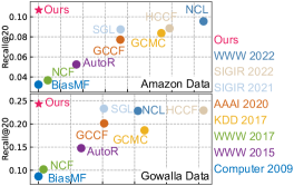
(a) Performance v.s. inference time

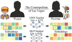
(b) Advantage of our adaptive embedding recalibration

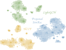
(c) Distribution of learned user embeddings

Figure 1. Illustration of motivation and advantages of our SimRec model from different perspectives.

Motivated examples showing the strength of SimRec from three aspects. Firstly, the proposed SimRec achieves best performance with less inference time. Secondly, our SimRec discovers the difference between a noisy user pair. Thirdly, SimRec learns embeddings preserving better user preference uniformly in comparison to baselines.

Having realized the importance of addressing the above challenges, however, it is non-trivial considering the following factors:

• How to well preserve global collaborative signals in an efficient manner for user-item interaction modeling, remains a challenge.

• How to encode informative representations which are robust to over-smoothing and noise issues while preserving high-order interaction patterns, requiring adaptive knowledge transfer.

As shown in Figure 1, we illustrate motivation examples for the model design in our SimRec recommender. To be specific, by comparing our SimRec with various state-of-the-art GNN-based CF methods (e.g., GCCF (chen2020revisiting), SGL (wu2021self), HCCF (xia2022hypergraph)) in Figure 1(a), SimRec significantly improves model efficiency, meanwhile maintaining superior recommendation performance. In Figure 1(b) of two users with dissimilar interests, we show the advantage of our adaptive contrastive knowledge distillation to recalibrate the similar representations encoded by GNN teacher model into distinguishable embedding space. To reflect the better uniformity preserved in learned embeddings of SimRec, we visualize the distributions of projected embeddings learned by different methods in Figure 1(c).

Inspired by the effectiveness of knowledge distillation (KD) in various domains (e.g., computer vision (zhang2021data), text mining (chen2020distilling), and graph mining (zhanggraph)), KD has become an effective solution to transfer knowledge from a large model to a smaller one. In general, KD aims to reach the agreement between the prediction results of a well-trained teacher model and a student model by minimizing their distribution difference. However, collaborative filtering task usually involves highly sparse interaction data, which undermines the capability of knowledge distillation. Specifically, direct distillation from noisy and sparse graph structures, is difficult to advance the performance of original GNN model after being compressed. Fortunately, recent developments of contrastive learning bring new insights in alleviating data sparsity with auxiliary self-supervision signals, this paper explores the possibility of marrying the power of knowledge distillation and contrastive learning to pursue adaptive knowledge transfer with a robust and efficient CF model.

In this work, we propose a novel graph-less collaborative filtering framework, named SimRec, to improve both the effectiveness and efficiency of recommender without the sophisticated GNN structures. In particular, we propose a bi-level alignment framework to distill knowledge with both prediction-level and embedding-level signals. With such design, the distilled knowledge comes from not only the teacher model’s predictions but also the latent high-order collaborative semantics preserved in embeddings. Furthermore, we propose to enhance our knowledge distillation paradigm against the perturbation of over-smoothing and noise effects in GNN teacher model. Towards this end, an adaptive knowledge transfer module is designed with contrastive regularization to capture the diversity of user preference, based on the derived consistency between the supervised CF objective and the augmented SSL task. In our proposed SimRec model, the latent knowledge of GNN-based teacher model will be distilled into a lightweight yet empowered feed-forward network that can jointly capture user-specific preference uniformity and cross-user global collaborative dependencies.

To summarize, our contributions are presented as follows:

• We propose contrastive knowledge distillation to compress GNN-based CF model into a simple recommender to improve both effectiveness and efficiency. In our adaptive distillation paradigm, an embedding calibration module is designed to enhance KD to preserve useful knowledge and discard the noisy information.

• Theoretical analysis is provided from two perspectives: i) the benefits of our distillation model in alleviating over-smoothing issue; ii) effectiveness of our distilled self-supervision signals for data augmentation in an adaptive manner.

• Extensive experiments on public datasets demonstrate that SimRec significantly improves the performance of CF tasks. Additionally, the empirical results show that SimRec gains more efficient embedding encoding over LightGCN on different datasets.

2. Collaborative Filtering

In this section, we introduce important notations in collaborative filtering, and recap MLP-based Neural CF and GNN-based CF architectures. In a typical recommendation scenario, there are $I$ users $\{u_{1},u_{2},...,u_{I}\}$ and $J$ items $\{v_{1},v_{2},...,v_{J}\}$, indexed by $u_{i}$ and $v_{j}$, respectively. An interaction matrix $\textbf{A}\in\mathbb{R}^{I\times J}$ represents the observed interactions between users and items, in which an element $a_{i,j}=1$ if user $u_{i}$ has adopted item $v_{j}$, otherwise $a_{i,j}=0$.

Based on the above definitions, a CF-based recommender can be formalized as an inference model that i) Inputs the user-item interaction data $\textbf{A}\in\mathbb{R}^{I\times J}$, models users’ interactive patterns based on the input; ii) Outputs interaction prediction results $y_{i,j}$ between the unobserved user-item pair $(u_{i},v_{j})$. In general, a CF model can be summarized as the following two-stage schema:

(1) $$y_{i,j}\leftarrow\textbf{Predict}(\textbf{h}_{i},\textbf{h}_{j}),\leavevmode\nobreak\ \leavevmode\nobreak\ \leavevmode\nobreak\ \leavevmode\nobreak\ \textbf{h}_{i},\textbf{h}_{j}\leftarrow\textbf{Embed}(u_{i},v_{j};\textbf{A})$$

The first stage $\textbf{Embed}(\cdot)$ denotes the embedding process which projects user $u_{i}$ and item $v_{j}$ into a $d$-dimensional hidden space based on the observed historical interactions A. The results of $\textbf{Embed}(\cdot)$ is vectorized representations $\textbf{h}_{i},\textbf{h}_{j}\in\mathbb{R}^{d}$ for each user $u_{i}$ and item $v_{j}$, to preserve user-item interactive patterns. The second stage $\textbf{Predict}(\cdot)$ aims to forecast user-item relations with the prediction score $y_{i,j}\in\mathbb{R}$ using the learned embeddings $\textbf{h}_{i},\textbf{h}_{j}$. Based on the above two-stage schema, our proposed method SimRec aims to conduct knowledge distillation from both the embedding and prediction levels for effectively knowledge transferring.

MLP-based Collaborative Filtering. MLP-based neural CF methods (he2017neural; xue2017deep) are proposed to endow CF with non-linear relation modeling. Due to the simplicity in model architectures, MLP-based CF is highly-efficient and unlikely to learn over-smoothed emebddings like GNNs (chen2020measuring). Inspired by the advantages, we adopt MLP as the student model in our contrastive KD framework. In brief, the MLP in SimRec adheres to the two-stage paradigm as follows:

(2) $$y_{i,j}=\textbf{h}_{i}^{\top}\textbf{h}_{j},\leavevmode\nobreak\ \leavevmode\nobreak\ \leavevmode\nobreak\ \textbf{h}_{i}=\textbf{M-Embed}(\bar{\textbf{h}}_{i}),\leavevmode\nobreak\ \leavevmode\nobreak\ \leavevmode\nobreak\ \textbf{h}_{j}=\textbf{M-Embed}(\bar{\textbf{h}}_{j})$$

where $\bar{\textbf{h}}_{i},\bar{\textbf{h}}_{j}\in\mathbb{R}^{d}$ denote the initial embedding vectors for user $u_{i}$ and item $v_{j}$, respectively. $\textbf{M-Embed}(\cdot)$ denotes the MLP-based embedding function. We adopt dot-product for $\textbf{Predict}(\cdot)$, which has been shown to be efficient and effective (rendle2020neural).

GNN-enhanced Collaborative Filtering. Most recent CF models apply graph neural information propagation on a bipartite interaction graph $\mathcal{G}=\{\mathcal{U},\mathcal{V},\mathcal{E}\}$, to encode users’ high-order interactive relations into node embeddings. Here, $\mathcal{U}=\{u_{i}\},\mathcal{V}=\{v_{j}\}$ denote user and item node sets, respectively. An edge $e_{i,j}\in\mathcal{E}$ exists if and only if $a_{i,j}=1$. Typically, GNN-based CF can be abstracted as:

(3) $$y_{i,j}=\textbf{h}_{i}^{\top}\textbf{h}_{j},\leavevmode\nobreak\ \textbf{H}=\textbf{G-Embed}(\mathcal{G},\bar{\textbf{H}})=\left(\textbf{Agg}(\textbf{Prop}(\mathcal{G},\bar{\textbf{H}}))\right)^{L}$$

where $\textbf{H},\bar{\textbf{H}}\in\mathbb{R}^{(I+J)\times d}$ denote the embedding matrices whose rows are node embedding vectors. $\textbf{G-Embed}(\cdot)$ denotes the GNN-based embedding function which iteratively propagates ($\textbf{Prop}(\cdot)$) and aggregates ($\textbf{Agg}(\cdot)$) the embeddings $\bar{\textbf{H}}$ along the interaction graph $\mathcal{G}$ for $L$ times. Note that though it injects informative structural information, GNNs based on holistic graph modeling and high-order iterations also damage the model scalability and bring the risk of over-smoothing in the collaborative filtering task.

3. Methodology

In this section, we elaborate the technical details of our proposed SimRec framework, whose workflow is depicted in Figure 2.

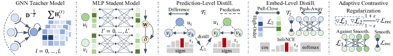
Figure 2. Model architecture of the proposed SimRec framework.

The architecture of the proposed SimRec model, consisting the GNN teacher, the MLP student, and the bi-level alignment: the prediction-level and the embedding-level knowledge distillation.

3.1. Contrastive Knowledge Distillation

For the model design, we are motivated by the advantages of i) GNNs in learning structure-aware node embeddings, and ii) efficient MLPs in preventing over-smoothing issue. Towards this end, we propose to distill knowledge from a GNN-based teacher model to a MLP-based student model. Specifically, the teacher model is a lightweight Graph Convolutional Network (GCN) (he2020lightgcn; wu2021self; cailightgcl) whose embedding process is shown with the following propagation:

(4) $$\textbf{H}^{(t)}=\sum_{l=0}^{L}\textbf{H}^{(t)}_{l},\leavevmode\nobreak\ \leavevmode\nobreak\ \leavevmode\nobreak\ \textbf{H}^{(t)}_{l+1}=\textbf{D}^{-\frac{1}{2}}(\bar{\textbf{A}}+\textbf{I})\textbf{D}^{-\frac{1}{2}}\cdot\textbf{H}^{(t)}_{l}$$

where $\textbf{H}^{(t)}\in\mathbb{R}^{(I+J)\times d}$ denotes the embedding matrix given by the teacher model. Index $l$ indicates the number of graph neural iterations (totally $L$ iterations). $\bar{\textbf{A}}\in\mathbb{R}^{(I+J)\times(I+J)}$ denotes the symmetric adjacent matrix for graph $\mathcal{G}$ generated from the interaction matrix A  (wang2019neural). I denotes the identity matrix, and D denotes the diagonal degree matrix of $\bar{\textbf{A}}$. The iteration is initialized by $\textbf{H}^{(t)}_{0}=\bar{\textbf{H}}^{(t)}$. The student model uses a shared MLP network to extract features from the initial embeddings for both users and items. For user $u_{i}$, the embedding layer is formally presented as follows:

(5) $$\textbf{h}^{(s)}_{i}=\textbf{FC}^{L^{\prime}}(\bar{\textbf{h}}^{(s)}_{i}),\leavevmode\nobreak\ \leavevmode\nobreak\ \leavevmode\nobreak\ \leavevmode\nobreak\ \textbf{FC}(\bar{\textbf{h}}^{(s)}_{i})=\delta(\textbf{W}\bar{\textbf{h}}^{(s)}_{i})+\bar{\textbf{h}}^{(s)}_{i}$$

where $\textbf{h}_{i}^{(s)},\bar{\textbf{h}}_{i}^{(s)}\in\mathbb{R}^{d}$ denote embeddings for $u_{i}$ given by the student. $\textbf{FC}(\cdot)$ denotes the fully-connected layer. $L^{\prime}$ is the number of FC layers. An FC layer is configured with one transformation $\textbf{W}\in\mathbb{R}^{d\times d}$. LeakyReLU activation $\delta(\cdot)$, and a residual connection (he2016deep) are applied. Item-side embedding layer is built analogously.

3.1.1. Prediction-Level Distillation

To distill knowledge from the teacher model to the student model, SimRec first follows the paradigm of KL-divergence-based KD (hinton2015distilling) to align the predictive outputs between the teacher and student models. Inspired by the success of ranking-oriented BPR loss (rendle2009bpr) in recommender systems, SimRec aligns the two models on the task of ranking user preference. Specifically, in each training step, we randomly sample a batch of triplets $\mathcal{T}_{1}=\{(u_{i},v_{j},v_{k})\}$, where $u_{i},v_{j},v_{k}$ are individually sampled from the holistic user and item set with uniform probability. Then SimRec calculates the preference difference between $(u_{i},v_{j})$ and $(u_{i},v_{k})$ for both models, as follows:

(6) $$z_{i,j,k}=y_{i,j}-y_{i,k}=\textbf{h}_{i}^{\top}\textbf{h}_{j}-\textbf{h}_{i}^{\top}\textbf{h}_{k}$$

where $z_{i,j,k}\in\mathbb{R}$ denotes the difference scores of user preferences for triplet $(u_{i},v_{j},v_{k})$. We denote the score given by the student model as $z_{i,j,k}^{(s)}$ and denote the score given by the teacher model as $z_{i,j,k}^{(t)}$. Then, the prediction-oriented distillation is conducted by minimizing the following loss function:

$$\mathcal{L}_{1}= \sum\limits_{(u_{i},v_{j},v_{k})\in\mathcal{T}_{1}}-\left(\bar{z}_{i,j,k}^{(t)}\cdot\log\bar{z}_{i,j,k}^{(s)}+(1-\bar{z}_{i,j,k}^{(t)})\cdot\log(1-\bar{z}_{i,j,k}^{(s)})\right)$$

(7) $$\bar{z}_{i,j,k}^{(t)}=\text{sigm}(z_{i,j,k}^{(t)}/\tau_{1}),\leavevmode\nobreak\ \leavevmode\nobreak\ \leavevmode\nobreak\ \leavevmode\nobreak\ \leavevmode\nobreak\ \bar{z}_{i,j,k}^{(s)}=\text{sigm}(z_{i,j,k}^{(s)}/\tau_{1})$$

where $\bar{z}_{i,j,k}^{(t)},\bar{z}_{i,j,k}^{(s)}$ are preference differences processed by sigmoid function $\text{sigm}(\cdot)$ with temperature factor $\tau_{1}$. Here, $z_{i,j,k}^{(t)}$ is given by well-trained teacher model and does not back-propagate gradients. With the help of prediction-oriented distillation $\mathcal{L}_{1}$, simple MLPs learn to mimic the predictions of advanced GNN models and thus directly generate recommendation results. Through this end-to-end supervision, the parameters of student model are optimized to preserve the knowledge distilled from the teacher model.

It is worth noting that, our prediction-level KD differs from vanilla KD in its training sample enrichment for deep dark knowledge learning (saputra2019distilling; clark2019bam) in CF. Specifically, vanilla KD for multi-class classification (hinton2015distilling) mines dark knowledge from not only the class with highest score, but also from the ranks for all classes. However, treating CF as multi-classification is problematic, as there are too many classes (items), such that the soft labels easily approach zero and become hard to rank. To solve it, our prediction-level KD adopts the pair-wise ranking task instead, and excavates the dark knowledge by distilling from enriched samples. Unlike BPR-based model training which pairs each positive item with one negative item, our KD scheme learns from the teacher’s predictions on $v_{j},v_{k}$ individually sampled from the holistic item set. Here $v_{j},v_{k}$ are not fixed to be positive or negative. This greatly enriches the training set for our KD and facilitate deeper dark knowledge distillation.

3.1.2. Embedding-Level Distillation

Despite the efficacy, the above prediction-level distillation only supervises the model outputs, but ignores the potential difference of embedding distributions between the student and teacher. As both models follow the embedding and prediction schema in Eq 1, we extend the KD paradigm in SimRec with an embedding-level knowledge transferring based on contrastive learning. Specifically, we sample a batch of users and items $\mathcal{T}_{2}=\{u_{i},v_{j}\}$ from the observed interactions in each training step. Then, we apply the following contrastive loss on the corresponding user/item embeddings:

$$\mathcal{L}_{2} =\sum_{u_{i}\in\mathcal{T}_{2}}-\log\frac{\exp\left(\cos(\textbf{h}^{(s)}_{i},\sum_{l=2}^{L}\textbf{h}^{(t)}_{i,l})/\tau_{2}\right)}{\sum_{u_{i^{\prime}}\in\mathcal{U}}\exp\left(\cos(\textbf{h}^{(s)}_{i^{\prime}},\sum_{l=2}^{L}\textbf{h}^{(t)}_{i,l})/\tau_{2}\right)}$$

(8) $$+\sum_{v_{j}\in\mathcal{T}_{2}}-\log\frac{\exp\left(\cos(\textbf{h}^{(s)}_{j},\sum_{l=2}^{L}\textbf{h}^{(t)}_{j,l})/\tau_{2}\right)}{\sum_{v_{j^{\prime}}\in\mathcal{V}}\exp\left(\cos(\textbf{h}^{(s)}_{j^{\prime}},\sum_{l=2}^{L}\textbf{h}^{(t)}_{j,l})/\tau_{2}\right)}$$

where $\cos(\cdot)$ denotes the cosine similarity function. $\tau_{2}$ represents the temperature hyperparameter. To force the student model to learn more from the high-order patterns which MLP-based CF lacks, here we only use the high-order node embeddings from the teacher. Embeddings of the teacher are well-trained and fixed in parameter optimization. Through directly regularizing the hidden embeddings with this embedding-oriented distillation, SimRec not only further improves the performance of student model, but also greatly accelerates the cross-model distillation, which has been validated in our empirical evaluations.

3.2. Adaptive Contrastive Regularization

To prevent transferring over-smoothed signals from the GNN-based teacher to the student model, SimRec proposes to regularize the embedding learning of the student by universally minimizing the node-wise similarity. Specially, SimRec adaptively locates which nodes are more likely being over-smoothed by comparing the gradients of distillation tasks with the main task gradients. In particular, we reuse the sampled users and items $\mathcal{T}_{2}$ from the embedding-level distillation, and apply the following adaptive contrastive regularization for node embeddings of the student model:

$$\mathcal{L}_{3}= \sum_{u_{i}\in\mathcal{T}_{2}}\varphi(u_{i},\mathcal{U},\omega_{i})+\varphi(u_{i},\mathcal{V},\omega_{i})+\sum_{v_{j}\in\mathcal{T}_{2}}\varphi(v_{j},\mathcal{V},\omega_{j})$$

(9) $$\varphi(u_{i},\mathcal{U},\omega_{i})=\omega_{i}\cdot\log\sum_{u_{i^{\prime}}\in\mathcal{U}}\exp(\textbf{h}_{i}^{(s)\top}\textbf{h}_{i^{\prime}}^{(s)}/\tau_{3})$$

where the loss $\mathcal{L}_{3}$ is composed of three terms ($\varphi(\cdot)$) that pushes away the user-user distance, the user-item distance, and the item-item distance, respectively. The first term $\varphi(u_{i},\mathcal{U},\omega_{i})$ minimizes the dot-product similarity between the embedding of $u_{i}$ and the embedding of each user $u_{i^{\prime}}$ in $\mathcal{U}$, with a weighting factor $\omega_{i}$. Here, the similarity score is adjusted with the temperature hyperparameter $\tau_{3}$. The $\phi(\cdot)$ functions for user-item relations and item-item relations work analogously. The weighting factor $\omega_{i},\omega_{j}$ correspond to $u_{i},v_{j}$ respectively, and the weight is calculated as follows:

$$\omega_{i}=\left\{\begin{aligned} &1-\varepsilon\leavevmode\nobreak\ \leavevmode\nobreak\ \leavevmode\nobreak\ \leavevmode\nobreak\ \leavevmode\nobreak\ \text{if}\bigtriangledown_{i}^{1,2\top}\bigtriangledown_{i}^{\text{rec}}>\bigtriangledown_{i}^{1^{\top}}\bigtriangledown_{i}^{2}\\ &1+\varepsilon\leavevmode\nobreak\ \leavevmode\nobreak\ \leavevmode\nobreak\ \leavevmode\nobreak\ \leavevmode\nobreak\ \text{otherwise}\end{aligned}\right.\leavevmode\nobreak\ \leavevmode\nobreak\ \leavevmode\nobreak\ \leavevmode\nobreak\ \leavevmode\nobreak\ \bigtriangledown_{i}^{\text{rec}}=\frac{\partial\mathcal{L}_{\text{rec}}}{\partial\textbf{h}_{i}^{(s)}}$$

(10) $$\bigtriangledown_{i}^{1,2}=\frac{\partial(\mathcal{L}_{1}+\mathcal{L}_{2})}{\partial\textbf{h}_{i}^{(s)}},\leavevmode\nobreak\ \leavevmode\nobreak\ \leavevmode\nobreak\ \leavevmode\nobreak\ \leavevmode\nobreak\ \leavevmode\nobreak\ \bigtriangledown_{i}^{1}=\frac{\partial\mathcal{L}_{1}}{\partial\textbf{h}_{i}^{(s)}},\leavevmode\nobreak\ \leavevmode\nobreak\ \leavevmode\nobreak\ \leavevmode\nobreak\ \leavevmode\nobreak\ \leavevmode\nobreak\ \bigtriangledown_{i}^{2}=\frac{\partial\mathcal{L}_{2}}{\partial\textbf{h}_{i}^{(s)}}$$

where $\omega_{i}\in\mathbb{R}$ adjusts the weight of contrastive regularization for user $u_{i}$. In brief, $\omega_{i}$ has the larger value (i.e., $1+\epsilon$) when the gradients given by distillation tasks (which may over-smooth) contradict to the gradients generated by the main task (which hardly over-smooth). Here, $0<\epsilon<1$ is a hyperparameter. $\bigtriangledown_{i}\in\mathbb{R}^{d}$ denotes the gradients for the embedding vector $\textbf{h}_{i}$ w.r.t, different optimization tasks. For example, $\bigtriangledown_{i}^{1,2}$ denotes the compound gradients of the two distillation task objectives $\mathcal{L}_{1}$ and $\mathcal{L}_{2}$. $\bigtriangledown_{i}^{\text{rec}}$ denotes gradient of the recommendation task, which is independent to the GNN-based teacher and thus has no risk of over-smoothing. The task $\mathcal{L}_{\text{rec}}$ will be elaborated later. The similarity between the gradients is estimated using dot-product. When the similarity between the distillation tasks and the recommendation task, is larger than the similarity between two distillation tasks, we can assume that the difference in optimization between the distillation and the recommendation is small enough to weaken the regularization.

3.3. Parameter Learning of SimRec

Following the training paradigm of knowledge distillation, our SimRec first trains the GNN-based teacher model until convergence. In each step, SimRec samples a batch of triplets $\mathcal{T}_{\text{bpr}}=\{(u_{i},v_{j},v_{k})|a_{i,j}=1,a_{i,k}=0\}$ where $u_{i}$ denotes anchor user. $v_{j}$ and $v_{k}$ denotes positive item and negative item, respectively. The BPR loss function (rendle2009bpr) is applied on the sampled data as follows:

(11) $$\mathcal{L}^{(t)}=-\sum_{(u_{i},v_{j},v_{k})\in\mathcal{T}_{\text{bpr}}}\log\text{sigm}(y^{(t)}_{i,j}-y^{(t)}_{i,k})+\lambda^{(t)}\|\bar{\textbf{H}}^{(t)}\|_{\text{F}}^{2}$$

where the last term denotes the weight-decay regularization with weight $\lambda^{(t)}$ for preventing over-fitting.

Then, SimRec conducts joint training to optimize the parameters of the MLP-based student, during which the structure-aware node representations are distilled from advanced GNNs to over-smoothness-resistant MLPs. The training process is elaborated in LABEL:sec:learn_alg. Strengthened by the two distillation tasks and the regularization terms, the overall optimization objective is presented:

$$\mathcal{L}^{(s)} =\mathcal{L}_{\text{rec}}+\lambda_{1}\cdot\mathcal{L}_{1}+\lambda_{2}\cdot\mathcal{L}_{2}+\lambda_{3}\cdot\mathcal{L}_{3}+\lambda_{4}\cdot\mathcal{L}_{4}$$

(12) $$\mathcal{L}_{\text{rec}} =-\sum\nolimits_{(u_{i},v_{j})\in\mathcal{T}_{2}}y_{i,j},\leavevmode\nobreak\ \leavevmode\nobreak\ \leavevmode\nobreak\ \leavevmode\nobreak\ \leavevmode\nobreak\ \leavevmode\nobreak\ \leavevmode\nobreak\ \mathcal{L}_{4}=\|\bar{\textbf{H}}^{(s)}\|_{\text{F}}^{2}$$

where $\lambda_{1},\lambda_{2},\lambda_{3},\lambda_{4}$ are weights for different optimization terms. $\mathcal{T}_{2}$ denotes the aforementioned set containing user-item pairs sampled from the observed interactions $\mathcal{E}$. As the contrastive regularization $\mathcal{L}_{3}$ minimizes the similarity between negative user-item pairs, the recommendation objective $\mathcal{L}_{\text{rec}}$ only maximizes the similarity between positive user-item pairs. $\mathcal{L}_{4}$ denotes the weight-decay regularization for the MLP neural network.

3.4. Further Discussion of SimRec

3.4.1. Adaptive High-Order Smoothing via KD

An important strength of GNN-based CF lies in its ability to smooth user/item embeddings using their high-order neighbors. Through derivation, we show our method is able to perform the high-order smoothing in an adaptive manner. Detailed derivations are presented in LABEL:sec:embed_analysis. In brief, for our light-weight GCN teacher, the embedding parameters $\bar{\textbf{h}}_{i}^{(t)},\bar{\textbf{h}}_{j}^{(t)}$ of two nodes $n_{i},n_{j}$ (either user or item nodes) are smoothed using each other, when minimizing the following terms from the BPR loss $\mathcal{L}^{(t)}$ in Eq 11:

(13) $$\frac{\partial\mathcal{L}^{(t)}_{i,j}}{\partial\bar{\textbf{h}}_{i}^{(t)}} =\sum_{v_{k}}-\sigma\cdot\Big{(}\sum_{\mathcal{P}_{i,j}^{2L}}\prod_{(n_{a},n_{b})\in\mathcal{P}_{i,j}^{2L}}\frac{1}{\sqrt{d_{a}d_{b}}}\Big{)}\cdot\frac{\partial\bar{\textbf{h}}_{i}^{(t)\top}\bar{\textbf{h}}_{j}^{(t)}}{\partial\bar{\textbf{h}}_{i}^{(t)}}$$

where $\mathcal{L}_{i,j}^{(t)}$ denotes the terms that pull close the embeddings of $n_{i}$ and $n_{j}$ in loss $\mathcal{L}^{(t)}$. $\sigma\in(0,1)$ is a BPR-relevant factor. $\mathcal{P}_{i,j}^{2L}$ represents a possible path between $n_{i}$ and $n_{j}$ with maximum length $2L$. $d_{a},d_{b}$ denotes the node degrees of $n_{a}$ and $n_{b}$, respectively. Eq 13 reveals that GCNs smooth embeddings for high-order nodes with weighted gradients. The weights (i.e., the bracketed part) encode how closely nodes are connected via multi-hop graph walks. Similarly, we analyze the gradients from our prediction-level KD $\mathcal{L}_{1}$ over embedding parameters $\textbf{h}_{i}^{(s)}$, as follows:

(14) $$\frac{\partial\mathcal{L}_{i,j}^{(1)}}{\partial{\textbf{h}}_{i}^{(s)}}=\sum_{v_{k}}-\frac{1}{\tau_{1}}\cdot(\bar{z}_{i,j,k}^{(t)}-\bar{z}_{i,j,k}^{(s)})\cdot\frac{\partial\textbf{h}_{i}^{(s)\top}\textbf{h}_{j}^{(s)}}{\partial\textbf{h}_{i}^{(s)}}$$

where $\mathcal{L}_{i,j}^{(1)}$ denotes the part from $\mathcal{L}_{1}$ that maximizes the similarity between the embeddings of $n_{i}$ and $n_{j}$. Eq 14 shows that, by utilizing the prediction-level KD, our MLP-based student can also be supercharged with high-order embedding smoothing without the cumbersome holistic-graph information propagation. Furthermore, the weights for different node pairs (i.e., the bracketed part) are derived from a well-trained GCN model, instead of depending on handcrafted heuristic manners as in Eq 13. This makes our KD framework robust to the noise of observed graph structures.

3.4.2. Enriched Supervision Augmentation via KD

Recent works (wu2021self; lin2022improving; xia2022hypergraph) propose to address the noise and the sparsity problems of CF by providing self-supervision signals using contrastive learning (CL) techniques. We show that our KD approach can provide even more additional supervisions. Specifically, we list the pull-close gradients from both InfoNCE-based CL loss, and our KD loss $\mathcal{L}_{1}$, w.r.t, a single node embedding $\textbf{h}_{i}$, as follows:

$$\frac{\partial\mathcal{L}_{\text{CL}}}{\partial\textbf{h}_{i}} =-\frac{1}{\tau}\cdot\frac{\partial\textbf{h}_{i}^{{}^{\prime}\top}\textbf{h}^{\prime\prime}_{i}/(\|\textbf{h}^{\prime}_{i}\|_{2}\|\textbf{h}^{\prime\prime}_{i}\|_{2})}{\partial\textbf{h}_{i}}$$

(15) $$\frac{\partial\mathcal{L}_{1}}{\partial{\textbf{h}}_{i}^{(s)}} =\sum_{v_{j}}\frac{\partial\mathcal{L}_{i,j}^{(1)}}{\partial{\textbf{h}}_{i}^{(s)}}=\sum_{v_{j},v_{k}}-w_{i,j,k}\cdot\frac{\partial\textbf{h}_{i}^{(s)\top}\textbf{h}_{j}^{(s)}}{\partial\textbf{h}_{i}}$$

where $w_{i,j,k}$ represents the factors for simplicity. Shown by the second equation, our KD generates $|\{v_{j},v_{k}|(u_{i},v_{j},v_{k})\in\mathcal{T}_{2}\}|$ pull-close optimization terms for each node $u_{i}$, while CL method only generates one training sample. This evidently shows that our KD-based scheme can enrich the supplementary supervision signals, even without the data augmentation in CL (wu2021self).

3.4.3. Complexity Analysis

We analyze the complexity of SimRec to answer the following questions: i) How do GCNs compared to MLPs in efficiency? ii) How is the efficiency of our KD paradigm compared to state-of-the-art methods? Detailed analysis is presented in LABEL:sec:complexity_analysis. In concise, the computational complexity of the MLP network in SimRec is $\mathcal{O}(|\mathcal{T}_{2}|\times L^{\prime}\times d^{2})$, and the complexity of the GCN teacher is $\mathcal{O}(|\mathcal{E}|\times{L}\times d)$. The MLP student is more efficient to the GNN teacher. For the second question, the supplementary losses in SimRec takes $\mathcal{O}(|\mathcal{T}_{2}|\times(I+J)\times d)$ complexity, which is comparable to existing SSL collaborative filtering methods.

4. Evaluation

We conduct experiments from different aspects to validate the efficacy of the propose SimRec framework. The implementation details for our SimRec and the baseline methods are presented in LABEL:sec:implement. Our experiments aim to answer the following research questions:

• RQ1: How does the proposed SimRec perform on different experimental datasets in comparison to state-of-the-art baselines?

• RQ2: How does different sub-modules of the proposed SimRec framework contribute to the overall performance?

• RQ3: How scalabile is SimRec in handling large-scale data?

• RQ4: How does the model performance vary when tuning important hyperparameters of the proposed SimRec model?

• RQ5: How can our SimRec model address the over-smoothing issue compared with GNN-based recommendation methods?

4.1. Experimental Settings

4.1.1. Experimental Datasets

Table 1. Statistics of the experimental datasets.

Dataset	# Users	# Items	# Interactions	Interaction Density
Gowalla	25,557	19,747	294,983	$5.85\times 10^{-4}$
Yelp	42,712	26,822	182,357	$1.59\times 10^{-4}$
Amazon	76,469	83,761	966,680	$1.51\times 10^{-4}$

A table showing the statistics of the Gowalla data (25557 users, 19747 items, 294983 interactions), the Yelp data (42712 users, 26822 items, 182357 interactions), and the Amazon data (76469 users, 83761 items, 966680 interactions).

Table 2. Performance comparison on Gowalla, Yelp, and Amazon datasets in terms of Recall and NDCG.

Data	Metric	BiasMF	NCF	AutoR	PinSage	STGCN	GCMC	NGCF	GCCF	LightGCN	DGCF	SLRec	NCL	SGL	HCCF	SimRec	p-val.
Gowalla	Recall@20	0.0867	0.1019	0.1477	0.1235	0.1574	0.1863	0.1757	0.2012	0.2230	0.2055	0.2001	0.2283	0.2332	0.2293	0.2434	$2.1e^{-8}$
	NDCG@20	0.0579	0.0674	0.0690	0.0809	0.1042	0.1151	0.1135	0.1282	0.1433	0.1312	0.1298	0.1478	0.1509	0.1482	0.1592	$1.2e^{-9}$
	Recall@40	0.1269	0.1563	0.2511	0.1882	0.2318	0.2627	0.2586	0.2903	0.3181	0.2929	0.2863	0.3232	0.3251	0.3258	0.3399	$2.4e^{-8}$
	NDCG@40	0.0695	0.0833	0.0985	0.0994	0.1252	0.1390	0.1367	0.1532	0.1670	0.1555	0.1540	0.1745	0.1780	0.1751	0.1865	$1.7e^{-9}$
Yelp	Recall@20	0.0198	0.0304	0.0491	0.0510	0.0562	0.0584	0.0681	0.0742	0.0761	0.0700	0.0665	0.0806	0.0803	0.0789	0.0823	$3.7e^{-4}$
	NDCG@20	0.0094	0.0143	0.0222	0.0245	0.0282	0.0280	0.0336	0.0365	0.0373	0.0347	0.0327	0.0402	0.0398	0.0391	0.0414	$3.8e^{-5}$
	Recall@40	0.0307	0.0487	0.0692	0.0743	0.0856	0.0891	0.1019	0.1151	0.1175	0.1072	0.1032	0.1230	0.1226	0.1210	0.1251	$4.8e^{-3}$
	NDCG@40	0.0120	0.0187	0.0268	0.0315	0.0355	0.0360	0.0419	0.0466	0.0474	0.0437	0.0418	0.0505	0.0502	0.0492	0.0519	$2.4e^{-4}$
Amazon	Recall@20	0.0324	0.0367	0.0525	0.0486	0.0583	0.0837	0.0551	0.0772	0.0868	0.0617	0.0742	0.0955	0.0874	0.0885	0.1067	$1.1e^{-10}$
	NDCG@20	0.0211	0.0234	0.0318	0.0317	0.0377	0.0579	0.0353	0.0501	0.0571	0.0372	0.0480	0.0623	0.5690	0.0578	0.0734	$7.0e^{-12}$
	Recall@40	0.0578	0.0600	0.0826	0.0773	0.0908	0.1196	0.0876	0.1175	0.1285	0.0912	0.1123	0.1409	0.1312	0.1335	0.1535	$6.6e^{-10}$
	NDCG@40	0.0293	0.0306	0.0415	0.0402	0.0478	0.0692	0.0454	0.0625	0.0697	0.0468	0.0598	0.0764	0.0704	0.0716	0.0879	$2.0e^{-12}$

A table presenting the evaluated performance of the proposed SimRec model and the baselines, in which SimRec significantly outperforms the baseline methods.

Three benchmark datasets collected from real-world online services are used to evaluate the performance of SimRec. Data statistics are shown in Table 1. We split the interaction data into training set, validation set and test set with 70%:5%:25%. Details of the experimental datasets are:

• Gowalla: This dataset is collected from Gowalla, including user check-in records at geographical locations, from Jan to Jun, 2010.

• Yelp: This dataset contains users’ ratings on venues, collected from Yelp platform. The time range is from Jan to Jun, 2018.

• Amazon: This dataset is composed of users’ rating behaviors over books collected from Amazon platform, during 2013.

4.1.2. Evaluation Protocols

Following previous works on CF recommenders (wang2019neural; xia2022self), we conduct all-rank evaluation, in which positive items from test set are ranked with all un-interacted items for each user. The widely-used Recall@N and NDCG@N metrics (wu2021self; 2021knowledge) are used adopted for evaluation, where $N=20$ by default.

4.1.3. Baseline Models

We compare SimRec with the following 14 baselines from 4 research lines for comprehensive validation.
Traditional Collaborative Filtering Technique:

• BiasMF (koren2009matrix): It is a classic matrix factorization approach that combines user/item biases with learnable embedding vectors.

Non-GNN Neural Collaborative Filtering:

• NCF (he2017neural): It is an early study of deep learning CF model that enhances the user-item interaction modeling with MLP networks.

• AutoR (sedhain2015autorec): This method applies a three-layer autoencoder with fully-connected layers to encode user interaction vectors.

Graph Neural Architectures for Collaborative Filtering:

• PinSage (ying2018graph): This method combines random walk with graph convolutions for web-scale graph in recommendation.

• STGCN (zhang2019star): This method augments GCN with autoencoding sub-networks on hidden features for better inductive inference.

• GCMC (berg2017graph): This is a representative work to introduce graph convolutional operations into the matrix completion task.

• NGCF (wang2019neural): It is a GNN-based CF method which conducts graph convolutions on the user-item interaction graph for embeddings.

• GCCF (chen2020revisiting) and LightGCN(he2020lightgcn): These two methods propose to simplify conventional GCN structures by removing transformations and activations for improving performance.

Disentangled GNN-based Collaborative Filtering:

• DGCF(wang2020disentangled): This method disentangles user-item interactions into multiple hidden factors in the graph message passing process.

Self-Supervised Learning Approaches for Recommendation:

• SLRec (yao2021self): This method applies contrastive learning to recommendation models with feature-level data augmentations.

• NCL (lin2022improving): This approach enhances self-supervised graph CF models with enriched neighbor-wise contrastive learning.

• SGL (wu2021self): It conducts various types of graph augmentations and feature augmentations with graph contrastive learning for CF.

• HCCF (xia2022hypergraph): This method augments GNN-based CF with a global hypergraph GNN and conducts cross-view contrastive learning.

4.2. Overall Performance Comparison (RQ1)

The overall performance of SimRec and the baselines are shown in Table 2. From the results we have the following observations:

• Our SimRec consistently achieves best performance compared to baselines methods. Also, we re-train SimRec and the best-performed baselines (i.e., SGL and NCL) for 5 times to calculate $p$-values. The experimental results validate the significance of the improvement by SimRec. Compared to the state-of-the-art GNN methods, the MLP-based inference model of our graph-less SimRec generates more accurate recommendation results, due to its adaptive contrastive knowledge distillation. Specifically, the dual-level KD in SimRec enables enriched and adaptive high-order smoothing, which not only distills the accurate dark knowledge in the well-trained GNN teacher, but also avoids being affected by the over-smoothing signals. Furthermore, the adaptive contrastive regularization automatically alleviates the over-smoothing effects, which further boosts the performance.
  

• While the self-supervised learning schema greatly improves the performance of GNN-based CF, our graph-less SimRec model still significantly outperforms the SSL-enhanced graph models. We attribute the performance deficiency to the inherent incapability of existing SSL frameworks in filtering over-smoothing signals. For example, SGL augments model training by introducing random noises, which may even aggravate the inaccuracy in node embeddings when the noises are magnified through high-order graph propagation. As for NCL and HCCF, they seek to connect nodes based on global semantic relatedness, which may even over-smooth nodes distant from each other in the original graph. In comparison, our graph-less SimRec model abandons GNN architectures in the inference model, which fundamentally minimizes the possibility of over-smoothed node embeddings. Furthermore, our KD paradigm avoids distilling over-smoothed embeddings via the adaptive contrastive regularization.
  

• We observe that non-GNN CF models (i.e., NCF and AutoR) present very bad performance, event though they have similar MLP-based network architectures as the inference model in SimRec. This sheds light on the deficiency of MLPs in modeling high-order graph connectivity into user/item embeddings. While sharing similar MLP structures, our SimRec is additionally supervised by knowledge distilled from advanced GNN models. This not only improves the optimization for MLP networks, but also makes it possible to adaptively filter the over-smoothing signals in parameter learning. The huge performance gap between NCF/AutoR and our SimRec strongly shows the effectiveness of our contrastive knowledge distillation.

Table 3. Ablation study on key components of SimRec.

Data		Gowalla		Yelp		Amazon
Variant		Recall	NDCG	Recall	NDCG	Recall	NDCG
-$\mathcal{L}_{1}$		0.2180	0.1415	0.0756	0.0377	0.1012	0.0692
-$\mathcal{L}_{2}$	User	0.2292	0.1493	0.0806	0.0405	0.0998	0.0667
	Item	0.2266	0.1477	0.0808	0.0406	0.0974	0.0649
	Both	0.2222	0.1451	0.0787	0.0399	0.0938	0.0626
-$\mathcal{L}_{3}$	U-I	0.2330	0.1496	0.0814	0.0410	0.0939	0.0607
	U-U	0.2349	0.1512	0.0811	0.0407	0.0965	0.0634
	I-I	0.2331	0.1514	0.0813	0.0409	0.1009	0.0674
	All	0.2282	0.1480	0.0810	0.0407	0.0933	0.0605
SimRec		0.2434	0.1592	0.0823	0.0414	0.1067	0.0734

A table presenting the results of module ablation study. The results are divided into three parts: loss $\mathcal{L}_{1}$ for the prediction-level distillation, loss $\mathcal{L}_{2}$ for the embedding level distillation, and loss $\mathcal{L}_{3}$ for the contrastive regularization. All ablated variants performs worse than the proposed SimRec.