Corresponding author

Optimal investment in ambiguous financial markets with learning

Nicole Bäuerle Institute of Stochastics, Karlsruhe Institute of Technology (KIT), D-76128 Karlsruhe, Germany nicole.baeuerle@kit.edu  and  Antje Mahayni Mercator School of Management, University of Duisburg–Essen, Lotharstr. 65, 47057, Duisburg, Germany amahayni@uni-due.de missing
Abstract.

We consider the classical multi-asset Merton investment problem under drift uncertainty, i.e. the asset price dynamics are given by geometric Brownian motions with constant but unknown drift coefficients. The investor assumes a prior drift distribution and is able to learn by observing the asset prize realizations during the investment horizon. While the solution of an expected utility maximizing investor with constant relative risk aversion (CRRA) is well known, we consider the optimization problem under risk and ambiguity preferences by means of the KMM (Klibanoff et al., (2005)) approach. Here, the investor maximizes a double certainty equivalent. The inner certainty equivalent is for given drift coefficient, the outer is based on a drift distribution. Assuming also a CRRA type ambiguity function, it turns out that the optimal strategy can be stated in terms of the solution without ambiguity preferences but an adjusted drift distribution. To the best of our knowledge an explicit solution method in this setting is new. We rely on some duality theorems to prove our statements.
Based on our theoretical results, we are able to shed light on the impact of the prior drift distribution as well as the consequences of ambiguity preferences via the transfer to an adjusted drift distribution, i.e. we are able to explain the interaction of risk and ambiguity preferences. We compare our results with the ones in a pre-commitment setup where the investor is restricted to deterministic strategies. It turns out that (under risk and ambiguity aversion) an infinite investment horizon implies in both cases a maximin decision rule, i.e. the investor follows the worst (best) Merton fraction (over all realizations of it) if she is more (less) risk averse than a log-investor. We illustrate our findings with an extensive numerical study.

otsep5

Key words:

portfolio optimization, learning, smooth ambiguity, duality theory, Bayesian investment problem

JEL classifications:

C61, G11, D81

1. Introduction

We investigate the effects of model ambiguity preferences on optimal investment decisions in a multi asset Black Scholes market. Since the seminal paper by Ellsberg, (1961), we know that decision makers may have a non-neutral attitude towards model ambiguity. As a result, preferences are decomposed into risk preferences (based on known probabilities) and preferences concerning the degree of uncertainty about the (unknown) model parameters and are evaluated separately. This is in particular relevant for portfolio optimization problems. A recent literature suggests that model ambiguity is at least as prominent as risk in making investment decisions, see Chen and Epstein, (2002).

There are different ways to incorporate model ambiguity in decision making, like for example summarized in Guidolin and Rinaldi, (2013). In our setting, model ambiguity refers to the drift uncertainty in the dynamics of asset prices 111It is well-known that the drift of stock prices is notoriously difficult to estimate, Gennotte, (1986) and we apply the smooth ambiguity approach of Klibanoff et al., (2005) to deal with it. The risk in asset prices itself is evaluated by a utility function applied to the terminal wealth. Thus, the expected utility is itself a random variable (determined by the prior distribution of the drift parameters) which is evaluated by a second utility function (ambiguity function) capturing the model ambiguity. This approach allows for a separation of risk and ambiguity. As a result we end up with a stochastic optimization problem over a nested expectation which leads to non-linear expectations and the fact that we cannot solve the problem with a standard HJB approach. As in Balter et al., (2021) we assume that both the risk aversion and ambiguity aversion of the investor are described by (CRRA) power functions. While Balter et al., (2021) consider pre-commitment strategies, we take into account for the possibility that the investor is able to gradually learn about the drift by observing the asset price movements.

First of all, we contribute to the literature by analytically solving the portfolio optimization problem under drift uncertainty and learning while taking into account for both, risk and ambiguity preferences. To the best of our knowledge this has not yet been achieved before in our setting. We exploit the fact that the norm-like functions which appear in the concatenations of the certainty equivalents for risk and ambiguity allow for a specific dual representation. On the one hand, such a result should have been expected from previous research about the representation of smooth ambiguity, see Iwaki and Osaki, (2014), on the other hand it shows that smooth ambiguity is nothing else than a special kind of robust control. Indeed, we can think of the optimization problem as a classical Bayesian problem with adjusted prior probability distribution for the drift where the adjustment is computed in a second optimization problem. The attitude towards ambiguity depends on the relation of the levels of risk and ambiguity aversion (Balter et al., (2021), Iwaki and Osaki, (2014)). Our quasi closed form solutions allow an in depth analysis of the interaction of risk and ambiguity preferences. Among others it turns out that with relatively increasing ambiguity aversion, the prior distribution is smoothly shifted from ’good’ to ’bad’ drift scenarios, i.e. an ambiguity averse decision maker is more pessimistic.

Second, we are able to determine the long-time behavior of an ambiguity neutral/averse Bayes investor in the multi asset case. This is much more challenging than in the single-asset case. There it has been shown in Bäuerle and Grether, (2017) that the worst/best drift is crucial. In the vector-valued case it is not clear which drift scenarios are worst and which best cases. It turns out that these extreme scenarios are determined by the Euclidean norm of the possible drift vectors. An investor who is more (less) risk averse than a log-investor 222investor with logarithmic ultility then tends to a maximin (maximax) decision rule (which does not depend on the probability distribution of the drift). More precisely, an infinite investment horizon implies that the more (less) risk averse investor initially acts as someone who knows that the drift belongs to the worst (best) case scenario. Relying on this result we are able to compare the optimal strategy under learning with pre-commitment strategies, i.e. strategies where the investor is restricted to strategies which are deterministic functions of time. We are able to explain why (compared to a pre-commitment strategy) the value of learning is rather low, even in the case of high investment horizons. For short investment horizons (or remaining investment horizons), the investor is not able to learn much about the drift. For long investment horizons, both investors are initially guided by the worst (best) scenario. Finally this observation also carries over to the investor with model ambiguity since she essentially behaves like a Bayesian investor with adjusted prior which does not play a role when a large time horizon is present. This is maybe expected since a large time horizon allows for perfectly learning the model.

Related literature:
Bayes optimization problems and their sensitivity: We treat the fact that the asset drifts or market prices of risk are unknown as a Bayesian problem where we have a prior distribution (knowledge) about the values of the parameters which are here the drift or equivalently the market price of risk. The observations of the asset prices can then be used to update the belief which is also known as learning. This is done with the help of a filter. This filter then becomes part of the state process of the optimization problem. Techniques like these are well-known in finance, see e.g. Lakner, (1995) Brennan, (1998), Karatzas and Zhao, (2001), Honda, (2003), Rieder and Bäuerle, (2005), Björk et al., (2010) for investment problems in Black Scholes markets. The sensitivity of the optimal investment strategy in a single-asset Bayesian Black Scholes model w.r.t. model parameters is an interesting topic and investigated among others in Rieder and Bäuerle, (2005), Longo and Mainini, (2016), Bäuerle and Grether, (2017).

Duality and ambiguity: One early approach to deal with ambiguity is to consider robust approaches, e.g. Gilboa and Schmeidler, (2004); Hansen and Sargent, (2001) and in continuous time control problems with ambiguous interest rates Lin and Riedel, (2021) and in semimartingale markets Schied, (2007), Schied et al., (2009). The latter survey paper discusses different robust formulations and their connection to risk measures. Robust approaches care about worst-case scenarios and have sometimes been criticised for being too pessimistic. Thus, Klibanoff et al., (2005) introduced smooth ambiguity (KMM) which weights possible scenarios in a smooth way. Using Yaari’s duality theory (Yaari, (1987)), Iwaki and Osaki, (2014) already showed that there is a dual approach to smooth ambiguity which connects the ’smoothing function’ to some distorted probabilities. The dual representation of entropic risk measures is used in Bäuerle and Rieder, (2020) to tackle discrete-time decision problems with exponential utility for the KMM ambiguity applied to an unknown parameter. In Skiadas, (2003, 2013) the author relates a robust control to a recursive utility approach.

Solving smooth ambiguity: Smooth ambiguity models are by definition more complex than standard decision models under uncertainty. There are not many explicitly solved cases and approaches to tackle the problem. A static two-asset problem is considered and solved directly in Gollier, (2011). In Balter et al., (2021), the authors treat a Black-Scholes market with one risky asset and restrict to deterministic strategies which excludes learning. In Guan and Li, (2022) the authors look for equilibrium strategies in a smooth ambiguity problem with investment in a single-asset Black Scholes market and reinsurance and the mean-variance criterion. The recent paper Guan et al., (2023) also considers equilibrium portfolio strategies for smooth ambiguity preferences.

Learning and ambiguity: The effect of learning under ambiguity has e.g. been investigated in Epstein and Schneider, (2007) among others with the help of dynamic variants of the Ellsberg problem. In Ju and Miao, (2012) a generalized recursive smooth ambiguity and the effects on learning are considered. Both references deal with problems in discrete time. Suzuki, (2018) generalizes the results in Ju and Miao, (2012) by taking a limit to continuous time. Whereas in Baillon et al., (2018) the effect of learning information on people’s attitudes toward ambiguity is investigated. Miao, (2009) considers optimal consumption and investment in a similar financial market with incomplete information, however apply a recursive multiple priors approach which immediately yields some kind of worst case problem over densities. Numerical results are not provided in the paper.

The outline of the paper is as follows. First, Section 2 states the optimization problem and its solution. We start with a multi-asset Black Scholes model where we set the interest rate to zero for simplicity. Then we review the classical Bayesian case and explain how the problem with ambiguity can be solved analytically. A main tool is Sion’s minimax theorem. Proofs are deferred to the appendix. Sec. 3 first analyzes the optimal strategy in the Bayesian model, since the optimal strategy in the ambiguous case boils down to this setting with adjusted prior. We discuss the behavior of the optimal investment strategy for short and long time horizon. The latter one being quite difficult to analyse. A particular focus is on the special case with two-point prior where we can represent the optimal investment strategy as a convex combination of Merton fractions which are optimal in the setting with complete information given by the two drift settings. We also consider the case with pre-commitment i.e. when the investment strategy has to be chosen at time 00 and compare the two cases. Finally we simplify in the two-prior scenario the problem with model ambiguity. In Section 4 we present an extensive numerical study which sheds further light on our theoretical statements and gives some intuitive explanations. We restrict here to the single-asset case and two-point prior. The appendix contains proofs and further parameter constellations not discussed in the main sections.

2. Optimization problem and solution

Let (Ω,,(t),)Ωsubscript𝑡(\Omega,\mathcal{F},(\mathcal{F}_{t}),\mathbb{P}) be a filtered probability space and T>0𝑇0T>0 be a finite time horizon. The underlying financial market consists of d𝑑d stocks and one riskless bond, each defined on the previously mentioned probability space. The price process S=(S1(t),,Sd(t))t[0,T]𝑆subscriptsubscript𝑆1𝑡subscript𝑆𝑑𝑡𝑡0𝑇S=(S_{1}(t),\ldots,S_{d}(t))_{t\in[0,T]} of the d𝑑d stocks will for i=1,,d𝑖1𝑑i=1,\ldots,d be given by

dSi(t)=Si(t)[μidt+j=1dσijdWj(t)]=Si(t)[j=1dσijdYj(t)],𝑑subscript𝑆𝑖𝑡subscript𝑆𝑖𝑡delimited-[]subscript𝜇𝑖𝑑𝑡superscriptsubscript𝑗1𝑑subscript𝜎𝑖𝑗𝑑subscript𝑊𝑗𝑡subscript𝑆𝑖𝑡delimited-[]superscriptsubscript𝑗1𝑑subscript𝜎𝑖𝑗𝑑subscript𝑌𝑗𝑡dS_{i}(t)=S_{i}(t)\left[\mu_{i}dt+\sum_{j=1}^{d}\sigma_{ij}dW_{j}(t)\right]=S_{i}(t)\left[\sum_{j=1}^{d}\sigma_{ij}dY_{j}(t)\right], (2.1)

where W=(W1(t),,Wd(t))t[0,T]𝑊subscriptsuperscriptsubscript𝑊1𝑡subscript𝑊𝑑𝑡top𝑡0𝑇W=(W_{1}(t),\ldots,W_{d}(t))^{\top}_{t\in[0,T]} is a d-dimensional Brownian motion, μi,σij+,i,j=1,,dformulae-sequencesubscript𝜇𝑖formulae-sequencesubscript𝜎𝑖𝑗subscript𝑖𝑗1𝑑\mu_{i}\in\mathbb{R},\sigma_{ij}\in\mathbb{R}_{+},i,j=1,\ldots,d and σ=(σij)𝜎subscript𝜎𝑖𝑗\sigma=(\sigma_{ij}) is regular. We further set

Y(t):=W(t)+Θt,Θ:=σ1μ,μ:=(μ1,,μd),formulae-sequenceassign𝑌𝑡𝑊𝑡Θ𝑡formulae-sequenceassignsuperscriptΘtopsuperscript𝜎1𝜇assign𝜇subscript𝜇1subscript𝜇𝑑Y(t):=W(t)+\Theta t,\quad\Theta^{\top}:=\sigma^{-1}\mu,\quad\mu:=(\mu_{1},\ldots,\mu_{d}),

where ΘΘ\Theta denotes the market price per unit of risk. The price process of the riskless bond is for simplicity assumed to be identical to 111.

We further assume that μ𝜇\mu is not known and thus a random variable. This implies that the market price of risk ΘΘ\Theta is also not known to the investor. However, she has a prior knowledge about ΘΘ\Theta in form of a prior distribution \mathbb{P} on dsuperscript𝑑\mathbb{R}^{d}. For the numerical part we assume that the random variable ΘΘ\Theta may take only one of the values ϑ1,,ϑmsubscriptitalic-ϑ1subscriptitalic-ϑ𝑚\vartheta_{1},\ldots,\vartheta_{m} with (Θ=ϑi)=piΘsubscriptitalic-ϑ𝑖subscript𝑝𝑖\mathbb{P}(\Theta=\vartheta_{i})=p_{i}.

In a next step we introduce a suitable set of trading strategies. Since the riskless bond is equal to 1 and we only consider self-financing strategies we can express the wealth process with the help of the investment in risky assets only. By π=(π1,,πd)𝜋subscript𝜋1subscript𝜋𝑑\pi=(\pi_{1},\ldots,\pi_{d}) we denote a d𝑑d-dimensional stochastic process representing the trading strategy of some investor, where πk(t)subscript𝜋𝑘𝑡\pi_{k}(t) describes the amount invested in the k𝑘k-th stock at time t[0,T]𝑡0𝑇t\in[0,T]. We denote by

Y(t):=σ(Y(s),0st),Y:=(Y(t))formulae-sequenceassignsuperscript𝑌𝑡𝜎𝑌𝑠0𝑠𝑡assignsuperscript𝑌superscript𝑌𝑡\mathcal{F}^{Y}(t):=\sigma(Y(s),0\leq s\leq t),\quad\mathcal{F}^{Y}:=(\mathcal{F}^{Y}(t))

the filtration generated by Y𝑌Y which is equivalent to the filtration generated by S𝑆S. Strategies π𝜋\pi should be Ysuperscript𝑌\mathcal{F}^{Y}-progressively measurable. This means that the agent is able to observe the stock prices and updates the belief about the market price of risk from this observation. In other words, the agent is able to learn the right market price of risk. The associated wealth process denoted by (Xtπ)t[0,T]subscriptsubscriptsuperscript𝑋𝜋𝑡𝑡0𝑇(X^{\pi}_{t})_{t\in[0,T]} is given by

dXtπ=k=1dπk(t)dSk(t)Sk(t)=π(t)σdY(t)𝑑subscriptsuperscript𝑋𝜋𝑡superscriptsubscript𝑘1𝑑subscript𝜋𝑘𝑡dsubscript𝑆𝑘𝑡subscript𝑆𝑘𝑡𝜋𝑡𝜎𝑑𝑌𝑡dX^{\pi}_{t}=\sum_{k=1}^{d}\pi_{k}(t)\frac{\mathrm{d}S_{k}(t)}{S_{k}(t)}=\pi(t)\sigma dY(t) (2.2)

with initial capital x0subscript𝑥0x_{0}\in\mathbb{R}. In what follows let

u(x)=1αxα,α<1,α0formulae-sequence𝑢𝑥1𝛼superscript𝑥𝛼formulae-sequence𝛼1𝛼0u(x)=\frac{1}{\alpha}x^{\alpha},\quad\alpha<1,\alpha\neq 0

be a CRRA utility function. The absolute and relative risk aversion is here given by

RA(x):=u′′(x)u(x)=1αx and RR(x):=xRA(x)=1α.assignsubscript𝑅𝐴𝑥superscript𝑢′′𝑥superscript𝑢𝑥1𝛼𝑥 and subscript𝑅𝑅𝑥assign𝑥subscript𝑅𝐴𝑥1𝛼\displaystyle R_{A}(x):=-\frac{u^{\prime\prime}(x)}{u^{\prime}(x)}=\frac{1-\alpha}{x}\text{ and }R_{R}(x):=xR_{A}(x)=1-\alpha.

It is well-known that the limiting case α0𝛼0\alpha\to 0 corresponds to the logarithmic utility.

2.1. The classical Bayesian case

The investor aims to maximize her expected utility of terminal wealth. First we assume that the investor is ambiguity-neutral w.r.t. the unknown parameter and consider

V(x0)=supπ𝔼ϑ[u(XTπ)](dϑ)𝑉subscript𝑥0subscriptsupremum𝜋subscript𝔼italic-ϑdelimited-[]𝑢superscriptsubscript𝑋𝑇𝜋𝑑italic-ϑV(x_{0})=\sup_{\pi}\int\mathbb{E}_{\vartheta}[u(X_{T}^{\pi})]\mathbb{P}(d\vartheta) (2.3)

where the supremum is taken over all Ysuperscript𝑌\mathcal{F}^{Y}-adapted strategies π𝜋\pi for which the stochastic integral and the expectations are defined and XTπ0superscriptsubscript𝑋𝑇𝜋0X_{T}^{\pi}\geq 0. We denote this set by 𝒜.𝒜\mathcal{A}. 𝔼ϑsubscript𝔼italic-ϑ\mathbb{E}_{\vartheta} is the conditional expectation, given Θ=ϑ.Θitalic-ϑ\Theta=\vartheta. This problem is the well-known Bayesian adaptive portfolio problem. We summarize its solution in the following theorem (Karatzas and Zhao, (2001); Rieder and Bäuerle, (2005)) (where \|\cdot\| is the usual Euclidean norm):

Theorem 2.1.

The maximal expected utility attained in (2.3) is given by

V(x0)=x0αα(dF(T,z)γφT(z)𝑑z)1/γ,x0>0formulae-sequence𝑉subscript𝑥0superscriptsubscript𝑥0𝛼𝛼superscriptsubscriptsuperscript𝑑𝐹superscript𝑇𝑧𝛾subscript𝜑𝑇𝑧differential-d𝑧1𝛾subscript𝑥00V(x_{0})=\frac{x_{0}^{\alpha}}{\alpha}\left(\int_{\mathbb{R}^{d}}F(T,z)^{\gamma}\varphi_{T}(z)dz\right)^{1/\gamma},\quad x_{0}>0 (2.4)

where γ=1/(1α)𝛾11𝛼\gamma=1/(1-\alpha), φTsubscript𝜑𝑇\varphi_{T} is the density of the d𝑑d-dimensional normal distribution 𝒩(0,TI)𝒩0𝑇𝐼\mathcal{N}(0,TI) (I𝐼I being the identity matrix) and for t0,zd,ϑformulae-sequence𝑡0formulae-sequence𝑧superscript𝑑italic-ϑt\geq 0,z\in\mathbb{R}^{d},\vartheta\in\mathbb{R} we define

F(t,z):=Lt(ϑ,z)(dϑ),Lt(ϑ,z):={exp(zϑ12ϑ2t)t>01t=0.formulae-sequenceassign𝐹𝑡𝑧subscript𝐿𝑡italic-ϑ𝑧𝑑italic-ϑassignsubscript𝐿𝑡italic-ϑ𝑧cases𝑧italic-ϑ12superscriptnormitalic-ϑ2𝑡𝑡01𝑡0F(t,z):=\int L_{t}(\vartheta,z)\mathbb{P}(d\vartheta),\quad L_{t}(\vartheta,z):=\left\{\begin{array}[]{ll}\exp{\big{(}z\cdot\vartheta-\frac{1}{2}\|\vartheta\|^{2}t\big{)}}&t>0\\ 1&t=0.\end{array}\right.\; (2.5)

The optimal fractions invested in the stocks are for t0𝑡0t\geq 0 given by

π(t)X(t)=γ(σ)1dF(T,z+Y(t))(F(T,z+Y(t))γ1φTt(z)dzd(F(T,z+Y(t))γφTt(z)dz\frac{\pi^{*}(t)}{X^{*}(t)}=\gamma(\sigma^{\top})^{-1}\frac{\int_{\mathbb{R}^{d}}\nabla F(T,z+Y(t))(F(T,z+Y(t))^{\gamma-1}\varphi_{T-t}(z)dz}{\int_{\mathbb{R}^{d}}(F(T,z+Y(t))^{\gamma}\varphi_{T-t}(z)dz} (2.6)

where Xsuperscript𝑋X^{*} is the wealth process under the optimal strategy π.superscript𝜋\pi^{*}.

Remark 2.2.
  • a)

    Recall in particular that in case the market price of risk is known and is equal to ϑ,italic-ϑ\vartheta, the optimal fractions which have to be invested do not depend on time and wealth and are given by

    π(t)X(t)=κMer(γ,ϑ):=γ(σ)1ϑ.superscript𝜋𝑡superscript𝑋𝑡superscript𝜅Mer𝛾italic-ϑassign𝛾superscriptsuperscript𝜎top1italic-ϑ\frac{\pi^{*}(t)}{X^{*}(t)}=\kappa^{\text{Mer}}(\gamma,\vartheta):=\gamma(\sigma^{\top})^{-1}\vartheta.

    This is a special case of our model when the prior distribution is concentrated on ϑ.italic-ϑ\vartheta. It is often named Merton fractions of a CRRA investor with a level of relative risk aversion 1γ=1α1𝛾1𝛼\frac{1}{\gamma}=1-\alpha. Indeed this fraction can be recovered from (2.6) as follows: Since the prior is concentrated on ϑitalic-ϑ\vartheta we obtain that F(t,z)=Lt(ϑ,z)𝐹𝑡𝑧subscript𝐿𝑡italic-ϑ𝑧F(t,z)=L_{t}(\vartheta,z) and thus

    π(t)X(t)=γ(σ)1dϑF(T,z+Y(t))(F(T,z+Y(t))γ1φTt(z)dzd(F(T,z+Y(t))γφTt(z)dz=γ(σ)1ϑ.\frac{\pi^{*}(t)}{X^{*}(t)}=\gamma(\sigma^{\top})^{-1}\frac{\int_{\mathbb{R}^{d}}\vartheta F(T,z+Y(t))(F(T,z+Y(t))^{\gamma-1}\varphi_{T-t}(z)dz}{\int_{\mathbb{R}^{d}}(F(T,z+Y(t))^{\gamma}\varphi_{T-t}(z)dz}=\gamma(\sigma^{\top})^{-1}\vartheta. (2.7)
  • b)

    In case α0𝛼0\alpha\to 0 which can be interpreted as the logarithmic utility we obtain that the optimal fractions invested in the stocks are for t0𝑡0t\geq 0 given by

    π(t)X(t)=(σ)1Θ^t=(σ)1𝔼[Θ|Y(t)]=(σ)1F(t,Y(t))F(t,Y(t)).superscript𝜋𝑡superscript𝑋𝑡superscriptsuperscript𝜎top1subscript^Θ𝑡superscriptsuperscript𝜎top1𝔼delimited-[]conditionalΘsuperscript𝑌𝑡superscriptsuperscript𝜎top1𝐹𝑡𝑌𝑡𝐹𝑡𝑌𝑡\frac{\pi^{*}(t)}{X^{*}(t)}=(\sigma^{\top})^{-1}\hat{\Theta}_{t}=(\sigma^{\top})^{-1}\mathbb{E}[\Theta|\mathcal{F}^{Y}(t)]=(\sigma^{\top})^{-1}\frac{\nabla F(t,Y(t))}{F(t,Y(t))}. (2.8)

    This is sometimes called certainty equivalence principle since the unknown market price of risk in the Merton fractions is simply replaced by its conditional expectation, given the information so far. The fraction here does not depend on the time horizon of investment. Moreover for discrete distribution \mathbb{P} on ϑ1,,ϑmsubscriptitalic-ϑ1subscriptitalic-ϑ𝑚\vartheta_{1},\ldots,\vartheta_{m} with (Θ=ϑi)=piΘsubscriptitalic-ϑ𝑖subscript𝑝𝑖\mathbb{P}(\Theta=\vartheta_{i})=p_{i}, it holds that

    (Θ=ϑi|Y(t))=piLi(ϑi,Y(t))F(t,Y(t)),i=1,,mformulae-sequenceΘconditionalsubscriptitalic-ϑ𝑖superscript𝑌𝑡subscript𝑝𝑖subscript𝐿𝑖subscriptitalic-ϑ𝑖𝑌𝑡𝐹𝑡𝑌𝑡𝑖1𝑚\mathbb{P}(\Theta=\vartheta_{i}|\mathcal{F}^{Y}(t))=\frac{p_{i}L_{i}(\vartheta_{i},Y(t))}{F(t,Y(t))},\quad i=1,\ldots,m

    is the conditional distribution of ΘΘ\Theta, Karatzas and Zhao, (2001); Rieder and Bäuerle, (2005). Also note that the expectation of Θ^tsubscript^Θ𝑡\hat{\Theta}_{t} remains constant over time and is thus equal to the expectation of the prior, since the process is a martingale by construction.

2.2. The case with model ambiguity concerns

Now we are interested in an investor who takes model ambiguity into account, i.e. instead of problem (2.3) we consider for a second utility function

v(x)=1λxλ,λ<1,λ0formulae-sequence𝑣𝑥1𝜆superscript𝑥𝜆formulae-sequence𝜆1𝜆0v(x)=\frac{1}{\lambda}\;x^{\lambda},\lambda<1,\lambda\neq 0

the problem (see e.g. Balter et al., (2021))

supπ𝒜v1vu1𝔼ϑ[u(XTπ)](dϑ)subscriptsupremum𝜋𝒜superscript𝑣1𝑣superscript𝑢1subscript𝔼italic-ϑdelimited-[]𝑢superscriptsubscript𝑋𝑇𝜋𝑑italic-ϑ\displaystyle\sup_{\pi\in\mathcal{A}}v^{-1}\int v\circ u^{-1}\mathbb{E}_{\vartheta}[u(X_{T}^{\pi})]\mathbb{P}(d\vartheta) (2.9)
=\displaystyle= supπ𝒜((𝔼ϑ[(XTπ)α])λ/α(dϑ))1/λsubscriptsupremum𝜋𝒜superscriptsuperscriptsubscript𝔼italic-ϑdelimited-[]superscriptsuperscriptsubscript𝑋𝑇𝜋𝛼𝜆𝛼𝑑italic-ϑ1𝜆\displaystyle\sup_{\pi\in\mathcal{A}}\left(\int\left(\mathbb{E}_{\vartheta}[(X_{T}^{\pi})^{\alpha}]\right)^{\lambda/\alpha}\mathbb{P}(d\vartheta)\right)^{1/\lambda}

This means that model ambiguity, represented by an uncertain market price of risk, is evaluated with a second utility function v𝑣v which is here of the same form but with possibly different parameter. In case α>0𝛼0\alpha>0 problem (2.9) is equivalent to

supπ𝒜(𝔼[(𝔼Θ[(XTπ)α])λ/α])α/λ,subscriptsupremum𝜋𝒜superscript𝔼delimited-[]superscriptsubscript𝔼Θdelimited-[]superscriptsuperscriptsubscript𝑋𝑇𝜋𝛼𝜆𝛼𝛼𝜆\sup_{\pi\in\mathcal{A}}\left(\mathbb{E}\left[\big{(}\mathbb{E}_{\Theta}[(X_{T}^{\pi})^{\alpha}]\big{)}^{\lambda/\alpha}\right]\right)^{\alpha/\lambda}, (2.10)

in case α<0𝛼0\alpha<0 it is equivalent to

infπ𝒜(𝔼[(𝔼Θ[(XTπ)α])λ/α])α/λ,subscriptinfimum𝜋𝒜superscript𝔼delimited-[]superscriptsubscript𝔼Θdelimited-[]superscriptsuperscriptsubscript𝑋𝑇𝜋𝛼𝜆𝛼𝛼𝜆\inf_{\pi\in\mathcal{A}}\left(\mathbb{E}\left[\big{(}\mathbb{E}_{\Theta}[(X_{T}^{\pi})^{\alpha}]\big{)}^{\lambda/\alpha}\right]\right)^{\alpha/\lambda}, (2.11)

In case α=λ𝛼𝜆\alpha=\lambda the problem reduces to the Bayesian problem discussed previously. Thus, if model risk and the market risk is evaluated with the same parameter we are back in the setting of Section 2.1. In what follows we restrict the discussion to the case α,λ(0,1).𝛼𝜆01\alpha,\lambda\in(0,1). The cases where at least one of the parameters is negative are similar and discussed in the appendix.

2.2.1. The ambiguity loving case

Let us now assume that λ>α>0𝜆𝛼0\lambda>\alpha>0 and define 𝐩:=λ/α>1assign𝐩𝜆𝛼1\mathbf{p}:=\lambda/\alpha>1. The economic interpretation is that the agent is less concerned about model ambiguity than about the risk in the stock market itself. In this case by using the L𝐩superscript𝐿𝐩L^{\mathbf{p}} norm 𝐩\|\cdot\|_{\mathbf{p}} we can write problem (2.10) as

supπ𝒜𝔼Θ[(XTπ)α]𝐩subscriptsupremum𝜋𝒜subscriptnormsubscript𝔼Θdelimited-[]superscriptsuperscriptsubscript𝑋𝑇𝜋𝛼𝐩\sup_{\pi\in\mathcal{A}}\left\|\mathbb{E}_{\Theta}[(X_{T}^{\pi})^{\alpha}]\right\|_{\mathbf{p}} (2.12)

where the norm is w.r.t. ΘΘ\Theta. It is well-known that the L𝐩superscript𝐿𝐩L^{\mathbf{p}} norm has the following dual representation for a r.v. X0𝑋0X\geq 0, where 1/𝐩+1/𝐪=11𝐩1𝐪11/\mathbf{p}+1/\mathbf{q}=1 (see e.g. Rudin, (1991)):

Lemma 2.3.

If 𝐩:=λ/α>1assign𝐩𝜆𝛼1\mathbf{p}:=\lambda/\alpha>1 we obtain for non-negative XL𝐩𝑋superscript𝐿𝐩X\in L^{\mathbf{p}}

X𝐩=sup{X𝑑:dd𝐪1}.subscriptnorm𝑋𝐩supremumconditional-set𝑋differential-dsubscriptnorm𝑑𝑑𝐪1\|X\|_{\mathbf{p}}=\sup\left\{\int Xd\mathbb{Q}:\left\|\frac{d\mathbb{Q}}{d\mathbb{P}}\right\|_{\mathbf{q}}\leq 1\right\}. (2.13)

where on the right-hand side of (2.13) the supremum is taken over all measures \mathbb{Q} (not necessarily probability measures) which are absolutely continuous w.r.t. \mathbb{P} and satisfy the constraint. Moreover, an optimal measure superscript\mathbb{Q}^{*} exists.

For a random variable X𝑋X with values {x1,,xm}subscript𝑥1subscript𝑥𝑚\{x_{1},\ldots,x_{m}\} and corresponding probabilities p1,,pdsubscript𝑝1subscript𝑝𝑑p_{1},\ldots,p_{d} we can thus write

(i=1mxi𝐩pi)1/𝐩=sup{i=1mxiqi:i=1m(qipi)𝐪pi1,qi0}.superscriptsuperscriptsubscript𝑖1𝑚superscriptsubscript𝑥𝑖𝐩subscript𝑝𝑖1𝐩supremumconditional-setsuperscriptsubscript𝑖1𝑚subscript𝑥𝑖subscript𝑞𝑖formulae-sequencesuperscriptsubscript𝑖1𝑚superscriptsubscript𝑞𝑖subscript𝑝𝑖𝐪subscript𝑝𝑖1subscript𝑞𝑖0\left(\sum_{i=1}^{m}x_{i}^{\mathbf{p}}p_{i}\right)^{1/\mathbf{p}}=\sup\left\{\sum_{i=1}^{m}x_{i}q_{i}:\sum_{i=1}^{m}\left(\frac{q_{i}}{p_{i}}\right)^{\mathbf{q}}p_{i}\leq 1,q_{i}\geq 0\right\}. (2.14)

In what follows define the set of measures 𝔔𝔔\mathfrak{Q} as the set of measures which satisfy the constraints in (2.13). This gives immediately rise to the following solution algorithm for our problem:

Theorem 2.4.

In the model of this subsection we have

supπ𝒜𝔼Θ[(XTπ)α]𝐩subscriptsupremum𝜋𝒜subscriptnormsubscript𝔼Θdelimited-[]superscriptsuperscriptsubscript𝑋𝑇𝜋𝛼𝐩\displaystyle\sup_{\pi\in\mathcal{A}}\left\|\mathbb{E}_{\Theta}[(X_{T}^{\pi})^{\alpha}]\right\|_{\mathbf{p}} =\displaystyle= supπ𝒜sup𝔔𝔼ϑ[(XTπ)α](dϑ)=sup𝔔supπ𝒜𝔼ϑ[(XTπ)α](dϑ)subscriptsupremum𝜋𝒜subscriptsupremum𝔔subscript𝔼italic-ϑdelimited-[]superscriptsuperscriptsubscript𝑋𝑇𝜋𝛼𝑑italic-ϑsubscriptsupremum𝔔subscriptsupremum𝜋𝒜subscript𝔼italic-ϑdelimited-[]superscriptsuperscriptsubscript𝑋𝑇𝜋𝛼𝑑italic-ϑ\displaystyle\sup_{\pi\in\mathcal{A}}\sup_{\mathbb{Q}\in\mathfrak{Q}}\int\mathbb{E}_{\vartheta}[(X_{T}^{\pi})^{\alpha}]\mathbb{Q}(d\vartheta)=\sup_{\mathbb{Q}\in\mathfrak{Q}}\sup_{\pi\in\mathcal{A}}\int\mathbb{E}_{\vartheta}[(X_{T}^{\pi})^{\alpha}]\mathbb{Q}(d\vartheta) (2.15)
=\displaystyle= 𝔼ϑ[(XTπ)α](dϑ).subscript𝔼italic-ϑdelimited-[]superscriptsuperscriptsubscript𝑋𝑇superscript𝜋𝛼superscript𝑑italic-ϑ\displaystyle\int\mathbb{E}_{\vartheta}[(X_{T}^{\pi^{*}})^{\alpha}]\mathbb{Q}^{*}(d\vartheta).

After normalizing \mathbb{Q}, the inner optimization problem is however, exactly the Bayesian portfolio problem of the previous section with distribution ~:=/()assign~\tilde{\mathbb{Q}}:=\mathbb{Q}/\mathbb{Q}(\mathbb{R}) for the unknown parameter. So solving (2.10) boils down to solving the classical Bayesian portfolio problem first with value given in Theorem 2.1 and then in a second step finding the optimal prior distribution implied by superscript\mathbb{Q}^{*} which is obtained from the outer optimization problem. The optimal strategy πsuperscript𝜋\pi^{*} is then the one in Theorem 2.1 with \mathbb{P} replaced by .superscript\mathbb{Q}^{*}.

2.2.2. The ambiguity averse case

Let us now assume that α>λ>0𝛼𝜆0\alpha>\lambda>0, i.e. the agent is more concerned about model ambiguity than about the risk in the financial market. This case is slightly more complicated. Define again 𝐩:=λ/α<1assign𝐩𝜆𝛼1\mathbf{p}:=\lambda/\alpha<1 and 𝐪𝐪\mathbf{q} by 1/𝐩+1/𝐪=11𝐩1𝐪11/\mathbf{p}+1/\mathbf{q}=1. Note that 𝐪<0𝐪0\mathbf{q}<0. We obtain (see Appendix 6.1):

Lemma 2.5.

If 𝐩:=λ/α<1assign𝐩𝜆𝛼1\mathbf{p}:=\lambda/\alpha<1 we obtain for non-negative XL1𝑋superscript𝐿1X\in L^{1}

(X𝐩𝑑)1/𝐩=inf{X𝑑:((dd)𝐪𝑑)1/𝐪1}.superscriptsuperscript𝑋𝐩differential-d1𝐩infimumconditional-set𝑋differential-dsuperscriptsuperscript𝑑𝑑𝐪differential-d1𝐪1\left(\int X^{\mathbf{p}}d\mathbb{P}\right)^{1/\mathbf{p}}=\inf\left\{\int Xd\mathbb{Q}:\Big{(}\int\Big{(}\frac{d\mathbb{Q}}{d\mathbb{P}}\Big{)}^{\mathbf{q}}d\mathbb{P}\Big{)}^{1/\mathbf{q}}\geq 1\right\}. (2.16)

where on the right-hand side of (2.16) the infimum is taken over all measures \mathbb{Q} (not necessarily probability measures) which are absolutely continuous w.r.t. \mathbb{P}. Moreover, an optimal measure superscript\mathbb{Q}^{*} exists.

In what follows we denote by 𝔔superscript𝔔\mathfrak{Q}^{\prime} the set of all measures which satisfy the constraints in (2.16) Hence we can write our optimization problem as

supπ𝒜(𝔼(𝔼Θ[(XTπ)α])𝐩)1𝐩=supπ𝒜inf𝔔𝔼ϑ[(XTπ)α](dϑ).subscriptsupremum𝜋𝒜superscript𝔼superscriptsubscript𝔼Θdelimited-[]superscriptsuperscriptsubscript𝑋𝑇𝜋𝛼𝐩1𝐩subscriptsupremum𝜋𝒜subscriptinfimumsuperscript𝔔subscript𝔼italic-ϑdelimited-[]superscriptsuperscriptsubscript𝑋𝑇𝜋𝛼𝑑italic-ϑ\sup_{\pi\in\mathcal{A}}\left(\mathbb{E}\left(\mathbb{E}_{\Theta}[(X_{T}^{\pi})^{\alpha}]\right)^{\mathbf{p}}\right)^{\frac{1}{\mathbf{p}}}=\sup_{\pi\in\mathcal{A}}\inf_{\mathbb{Q}\in\mathfrak{Q}^{\prime}}\int\mathbb{E}_{\vartheta}[(X_{T}^{\pi})^{\alpha}]\mathbb{Q}(d\vartheta). (2.17)

We have to show next that we can interchange the infimum and supremum in order to solve the problem as in the previous case. We proceed as in Bäuerle and Rieder, (2020) and use the following minimax theorem (see Sion, (1958)):

Theorem 2.6.

Let M𝑀M be any space and O𝑂O be a compact space, hh a function on M×O𝑀𝑂M\times O that is concave-convexlike. If h(x,y)𝑥𝑦h(x,y) is lower semi-continuous in y𝑦y for all xM𝑥𝑀x\in M then

supxinfyh(x,y)=infysupxh(x,y).subscriptsupremum𝑥subscriptinfimum𝑦𝑥𝑦subscriptinfimum𝑦subscriptsupremum𝑥𝑥𝑦\sup_{x}\inf_{y}h(x,y)=\inf_{y}\sup_{x}h(x,y).
Theorem 2.7.

In the model of this subsection where \mathbb{P} has compact support we have

supπ𝒜inf𝔔𝔼ϑ[(XTπ)α](dϑ)=inf𝔔supπ𝒜𝔼ϑ[(XTπ)α](dϑ)=𝔼ϑ[(XTπ)α](dϑ).subscriptsupremum𝜋𝒜subscriptinfimumsuperscript𝔔subscript𝔼italic-ϑdelimited-[]superscriptsuperscriptsubscript𝑋𝑇𝜋𝛼𝑑italic-ϑsubscriptinfimumsuperscript𝔔subscriptsupremum𝜋𝒜subscript𝔼italic-ϑdelimited-[]superscriptsuperscriptsubscript𝑋𝑇𝜋𝛼𝑑italic-ϑsubscript𝔼italic-ϑdelimited-[]superscriptsuperscriptsubscript𝑋𝑇superscript𝜋𝛼superscript𝑑italic-ϑ\sup_{\pi\in\mathcal{A}}\inf_{\mathbb{Q}\in\mathfrak{Q}^{\prime}}\int\mathbb{E}_{\vartheta}[(X_{T}^{\pi})^{\alpha}]\mathbb{Q}(d\vartheta)=\inf_{\mathbb{Q}\in\mathfrak{Q}^{\prime}}\sup_{\pi\in\mathcal{A}}\int\mathbb{E}_{\vartheta}[(X_{T}^{\pi})^{\alpha}]\mathbb{Q}(d\vartheta)=\int\mathbb{E}_{\vartheta}[(X_{T}^{\pi^{*}})^{\alpha}]\mathbb{Q}^{*}(d\vartheta). (2.18)

The solution procedure is then as in Theorem 2.4 by first solving the inner and then the outer problem.

Proof.

We apply Theorem 2.6 to the function L:𝒜×𝔔:𝐿𝒜superscript𝔔L:\mathcal{A}\times\mathfrak{Q}^{\prime}\to\mathbb{R} defined by

L(π,)=𝔼ϑ[(XTπ)α](dϑ).𝐿𝜋subscript𝔼italic-ϑdelimited-[]superscriptsuperscriptsubscript𝑋𝑇𝜋𝛼𝑑italic-ϑL(\pi,\mathbb{Q})=\int\mathbb{E}_{\vartheta}[(X_{T}^{\pi})^{\alpha}]\mathbb{Q}(d\vartheta).

where 𝒜𝒜\mathcal{A} is the set of admissible strategies. The set 𝔔superscript𝔔\mathfrak{Q}^{\prime} is not compact, however since we want to minimize over this set we can first restrict to a set 𝔔~~𝔔\mathfrak{\tilde{Q}} where the elements \mathbb{Q} have a mass bounded by a constant K>0𝐾0K>0. The proof of Lemma 2.5 shows that an optimal superscript\mathbb{Q}^{*} with finite mass exists. Next the mapping L(,π)maps-to𝐿𝜋\mathbb{Q}\mapsto L(\mathbb{Q},\pi) is linear and continuous w.r.t. weak convergence. Finally, since XTπsuperscriptsubscript𝑋𝑇𝜋X_{T}^{\pi} is linear in π𝜋\pi and xαsuperscript𝑥𝛼x^{\alpha} is concave, the mapping πL(,π)maps-to𝜋𝐿𝜋\pi\mapsto L(\mathbb{Q},\pi) is concave. Hence the assumptions are satisfied and Theorem 2.6 implies that we are able to interchange the infimum and supremum. ∎

Remark 2.8.

For simplicity we assume that our financial market is complete. However the approach to solve the smooth ambiguity problem by making use of a dual representation of the target function is independent of the precise formulation of the market. For example we could also solve smooth optimization problems in incomplete markets like in Karatzas et al., (1991) in the same way with the drawback that the solution of the inner optimization problem is more complicated and does not allow for such a nice formula as in Theorem 2.1.

Remark 2.9.

When we choose as utility function for our investor u(x)=eαx,α>0formulae-sequence𝑢𝑥superscript𝑒𝛼𝑥𝛼0u(x)=-e^{-\alpha x},\alpha>0 and for the ambiguity v(x)=eλx,λ>0formulae-sequence𝑣𝑥superscript𝑒𝜆𝑥𝜆0v(x)=-e^{-\lambda x},\lambda>0 then a quick calculation shows that vu1=(x)λ/α𝑣superscript𝑢1superscript𝑥𝜆𝛼v\circ u^{-1}=-(-x)^{\lambda/\alpha} and we can apply the same solution method in this case. However, the idea of the duality approach is more general. For example suppose that ambiguity aversion is smoothly measured via the negative of the entropic risk measure 1αln(𝔼[eαX]),α>01𝛼𝔼delimited-[]superscript𝑒𝛼𝑋𝛼0-\frac{1}{\alpha}\ln(\mathbb{E}[e^{-\alpha X}]),\alpha>0 and our decision maker is risk neutral. Then we would like to maximize

1αlneα𝔼ϑ[XTπ](dϑ)=inf{𝔼ϑ[XTπ](dϑ)+1αI(||)}-\frac{1}{\alpha}\ln\int e^{-\alpha\mathbb{E}_{\vartheta}[X_{T}^{\pi}]}\mathbb{Q}(d\vartheta)=\inf_{\mathbb{Q}}\left\{\int\mathbb{E}_{\vartheta}[X_{T}^{\pi}]\mathbb{Q}(d\vartheta)+\frac{1}{\alpha}I(\mathbb{Q}||\mathbb{P})\right\}

where the infimum is taken over all probability measures \mathbb{Q} which are absolutely continuous w.r.t. \mathbb{P} and I𝐼I is the usual relative entropy. This representation gives again rise to a decomposition of the problem in an inner and outer problem, Bäuerle and Rieder, (2020). Representations like this are well-known for convex risk measures, Schied, (2007).

3. Sensitivity and comparison results

In the previous section we have seen that solving the optimization problem with smooth ambiguity boils down to solving the classical Bayesian investment problem with the ’right’ prior distribution for the unknown market price of risk. In particular, as far as sensitivity results are concerned, the model behaves as the classical Bayesian problem. Thus, we first prove some sensitivity results for the classical case, i.e. for the optimal fractions in Theorem 2.1 which we denote by

κ(t,T,Y(t)):=π(t)X(t).assign𝜅𝑡𝑇𝑌𝑡superscript𝜋𝑡superscript𝑋𝑡\kappa(t,T,Y(t)):=\frac{\pi^{*}(t)}{X^{*}(t)}.

3.1. Limiting results for optimal investment fraction - General discrete prior

In what follows, suppose that the prior distribution \mathbb{P} is concentrated on ϑ1,,ϑmsubscriptitalic-ϑ1subscriptitalic-ϑ𝑚\vartheta_{1},\ldots,\vartheta_{m} with (Θ=ϑk)=pk,k=1,,mformulae-sequenceΘsubscriptitalic-ϑ𝑘subscript𝑝𝑘𝑘1𝑚\mathbb{P}(\Theta=\vartheta_{k})=p_{k},k=1,\ldots,m. The the i𝑖i-the row of (σ)1superscriptsuperscript𝜎top1(\sigma^{\top})^{-1} will be denoted by (σ)i1subscriptsuperscriptsuperscript𝜎top1𝑖(\sigma^{\top})^{-1}_{i} and \|\cdot\| is the usual Euclidean norm. When we assume that pk>0subscript𝑝𝑘0p_{k}>0 for all k𝑘k, we obtain the following results:

Theorem 3.1.

In the Bayesian model it holds for the optimal investment fractions:

  • a)

    for all y::𝑦absenty\in\mathbb{R}:

    limT0κ(0,T,y)=γ(σ)1k=1mϑkpk.subscript𝑇0𝜅0𝑇𝑦𝛾superscriptsuperscript𝜎top1superscriptsubscript𝑘1𝑚subscriptitalic-ϑ𝑘subscript𝑝𝑘\lim_{T\to 0}\kappa(0,T,y)=\gamma(\sigma^{\top})^{-1}\sum_{k=1}^{m}\vartheta_{k}p_{k}.
  • b)

    when ϑ1<<ϑmnormsubscriptitalic-ϑ1normsubscriptitalic-ϑ𝑚\|\vartheta_{1}\|<\ldots<\|\vartheta_{m}\| and α>0𝛼0\alpha>0 then for all t0𝑡0t\geq 0, y::𝑦absenty\in\mathbb{R}:

    limTκ(t,T,y)=γ(σ)1ϑm=κMer(γ,ϑm).subscript𝑇𝜅𝑡𝑇𝑦𝛾superscriptsuperscript𝜎top1subscriptitalic-ϑ𝑚superscript𝜅Mer𝛾subscriptitalic-ϑ𝑚\lim_{T\to\infty}\kappa(t,T,y)=\gamma(\sigma^{\top})^{-1}\cdot\vartheta_{m}=\kappa^{\text{Mer}}(\gamma,\vartheta_{m}).
  • c)

    when ϑ1<<ϑmnormsubscriptitalic-ϑ1normsubscriptitalic-ϑ𝑚\|\vartheta_{1}\|<\ldots<\|\vartheta_{m}\| and α<0𝛼0\alpha<0 then for all t0𝑡0t\geq 0, y::𝑦absenty\in\mathbb{R}:

    limTκ(t,T,y)=γ(σ)1ϑ1=κMer(γ,ϑ1).subscript𝑇𝜅𝑡𝑇𝑦𝛾superscriptsuperscript𝜎top1subscriptitalic-ϑ1superscript𝜅Mer𝛾subscriptitalic-ϑ1\lim_{T\to\infty}\kappa(t,T,y)=\gamma(\sigma^{\top})^{-1}\cdot\vartheta_{1}=\kappa^{\text{Mer}}(\gamma,\vartheta_{1}).
  • d)

    for all t0𝑡0t\geq 0, y𝑦y\in\mathbb{R} and i=1,,d::𝑖1𝑑absenti=1,\ldots,d:

    γmink{(σ)i1ϑk}κi(t,T,y)γmaxk{(σ)i1ϑk}.𝛾subscript𝑘subscriptsuperscriptsuperscript𝜎top1𝑖subscriptitalic-ϑ𝑘subscript𝜅𝑖𝑡𝑇𝑦𝛾subscript𝑘subscriptsuperscriptsuperscript𝜎top1𝑖subscriptitalic-ϑ𝑘\gamma\min_{k}\{(\sigma^{\top})^{-1}_{i}\cdot\vartheta_{k}\}\leq\kappa_{i}(t,T,y)\leq\gamma\max_{k}\{(\sigma^{\top})^{-1}_{i}\cdot\vartheta_{k}\}.
  • e)

    for all T>0𝑇0T>0:

    limα0κ(0,T,0)=(σ)1k=1mϑkpk.subscript𝛼0𝜅0𝑇0superscriptsuperscript𝜎top1superscriptsubscript𝑘1𝑚subscriptitalic-ϑ𝑘subscript𝑝𝑘\lim_{\alpha\downarrow 0}\kappa(0,T,0)=(\sigma^{\top})^{-1}\sum_{k=1}^{m}\vartheta_{k}p_{k}.

A proof of this theorem can be found in Appendix 6.2. Recall again that the limiting case α0𝛼0\alpha\to 0 corresponds to the logarithmic utility (cp. Rem. 2.2 b)) and the unknown market price of risk ΘΘ\Theta in the Merton fraction is simply replaced by its expectation e). The same is true, when the time horizon is short, see a). For a large time horizon, b), c) investors tend to extreme Merton fractions. In general the optimal investment fractions can be bounded by the entries in the Merton fractions, d).

Remark 3.2.

The statements are substantially easier to formulate and prove in the case when we have only one stock. In this case part a), d) and e) are special cases of Theorem 9 in Rieder and Bäuerle, (2005), part b) and c) are Theorem 3.1/3.3 in Bäuerle and Grether, (2017). Further sensitivity results in the one risky asset case can be found in Longo and Mainini, (2016).

3.2. Representation for optimal investment fraction - Two-point prior

Assume now further that μ=(μ1,,μd)𝜇subscript𝜇1subscript𝜇𝑑\mu=(\mu_{1},\ldots,\mu_{d}) can take only two possible (arbitrary) values μ¯=(μ¯1,,μ¯d)¯𝜇subscript¯𝜇1subscript¯𝜇𝑑\bar{\mu}=(\bar{\mu}_{1},\ldots,\bar{\mu}_{d}) and μ¯=(μ¯1,,μ¯d)¯𝜇subscript¯𝜇1subscript¯𝜇𝑑\underline{\mu}=(\underline{\mu}_{1},\ldots,\underline{\mu}_{d}). We assume that

(μ=μ¯)=p and (μ=μ¯)=1p,p(0,1).formulae-sequence𝜇¯𝜇𝑝 and 𝜇¯𝜇1𝑝𝑝01\mathbb{P}(\mu=\bar{\mu})=p\text{ and }\mathbb{P}(\mu=\underline{\mu})=1-p,\quad p\in(0,1). (3.1)

The optimization problem (2.3) boils down to

V(x0)=supπ𝒜p𝔼μ¯[u(XTπ)]+(1p)𝔼μ¯[u(XTπ)].𝑉subscript𝑥0subscriptsupremum𝜋𝒜𝑝subscript𝔼¯𝜇delimited-[]𝑢superscriptsubscript𝑋𝑇𝜋1𝑝subscript𝔼¯𝜇delimited-[]𝑢superscriptsubscript𝑋𝑇𝜋V(x_{0})=\sup_{\pi\in\mathcal{A}}\;p\mathbb{E}_{\bar{\mu}}[u(X_{T}^{\pi})]+(1-p)\mathbb{E}_{\underline{\mu}}[u(X_{T}^{\pi})]. (3.2)

where u(x)=1αxα.𝑢𝑥1𝛼superscript𝑥𝛼u(x)=\frac{1}{\alpha}x^{\alpha}. In this case the function F𝐹F appearing in (2.4) is given by F(t,z)=pLt(ϑ¯,z)+(1p)Lt(ϑ¯,z)𝐹𝑡𝑧𝑝subscript𝐿𝑡¯italic-ϑ𝑧1𝑝subscript𝐿𝑡¯italic-ϑ𝑧F(t,z)=pL_{t}(\bar{\vartheta},z)+(1-p)L_{t}(\underline{\vartheta},z). Let us further denote

F^(t,T,Y(t)):=LT(ϑ¯,z+Y(t))(F(T,z+Y(t)))γ1φTt(z)𝑑z(F(T,z+Y(t))γφTt(z)dz.\hat{F}(t,T,Y(t)):=\frac{\int_{\mathbb{R}}L_{T}(\underline{\vartheta},z+Y(t))(F(T,z+Y(t)))^{\gamma-1}\varphi_{T-t}(z)dz}{\int_{\mathbb{R}}(F(T,z+Y(t))^{\gamma}\varphi_{T-t}(z)dz}.

Then we can express the solution of (3.2) more explicitly.

Lemma 3.3.

In the case of a priori distribution of μ𝜇\mu given by (3.1), the optimal investment fractions κ(t,T,Y(t)):=π(t)X(t)assign𝜅𝑡𝑇𝑌𝑡superscript𝜋𝑡superscript𝑋𝑡\kappa(t,T,Y(t)):=\frac{\pi^{*}(t)}{X^{*}(t)} of the Bayesian problem (3.2) can be written as follows.

κ(t,T,Y(t))𝜅𝑡𝑇𝑌𝑡\displaystyle\kappa(t,T,Y(t)) =γ(σ)1ϑ¯α(t,T,Y(t))+γ(σ)1ϑ¯(1α(t,T,Y(t)))absent𝛾superscriptsuperscript𝜎top1¯italic-ϑ𝛼𝑡𝑇𝑌𝑡𝛾superscriptsuperscript𝜎top1¯italic-ϑ1𝛼𝑡𝑇𝑌𝑡\displaystyle=\gamma(\sigma^{\top})^{-1}\bar{\vartheta}\;\alpha(t,T,Y(t))+\gamma(\sigma^{\top})^{-1}\underline{\vartheta}\;(1-\alpha(t,T,Y(t)))
=κMer(γ,ϑ¯)α(t,T,Y(t))+κMer(γ,ϑ¯)(1α(t,T,Y(t)))absentsuperscript𝜅Mer𝛾¯italic-ϑ𝛼𝑡𝑇𝑌𝑡superscript𝜅Mer𝛾¯italic-ϑ1𝛼𝑡𝑇𝑌𝑡\displaystyle=\kappa^{\text{Mer}}(\gamma,\bar{\vartheta})\;\alpha(t,T,Y(t))+\kappa^{\text{Mer}}(\gamma,\underline{\vartheta})\;(1-\alpha(t,T,Y(t)))

with α(t,T,Y(t))=1(1p)F^(t,T,Y(t))[0,1].𝛼𝑡𝑇𝑌𝑡11𝑝^𝐹𝑡𝑇𝑌𝑡01\alpha(t,T,Y(t))=1-(1-p)\hat{F}(t,T,Y(t))\in[0,1].

Proof.

From Theorem 2.1 we know that the optimal fraction is given by:

κ(t,T,Y(t))=γ(σ)1dF(T,z+Y(t))(F(T,z+Y(t))γ1φTt(z)dzd(F(T,z+Y(t))γφTt(z)dz\kappa(t,T,Y(t))=\gamma(\sigma^{\top})^{-1}\frac{\int_{\mathbb{R}^{d}}\nabla F(T,z+Y(t))(F(T,z+Y(t))^{\gamma-1}\varphi_{T-t}(z)dz}{\int_{\mathbb{R}^{d}}(F(T,z+Y(t))^{\gamma}\varphi_{T-t}(z)dz} (3.3)

We obtain that

F(t,z)𝐹𝑡𝑧\displaystyle\nabla F(t,z) =pLt(ϑ¯,z)+(1p)Lt(ϑ¯,z)absent𝑝subscript𝐿𝑡¯italic-ϑ𝑧1𝑝subscript𝐿𝑡¯italic-ϑ𝑧\displaystyle=p\nabla L_{t}(\bar{\vartheta},z)+(1-p)\nabla L_{t}(\underline{\vartheta},z)
=pLt(ϑ¯,z)ϑ¯+(1p)Lt(ϑ¯,z)ϑ¯absent𝑝subscript𝐿𝑡¯italic-ϑ𝑧¯italic-ϑ1𝑝subscript𝐿𝑡¯italic-ϑ𝑧¯italic-ϑ\displaystyle=pL_{t}(\bar{\vartheta},z)\bar{\vartheta}+(1-p)L_{t}(\underline{\vartheta},z)\underline{\vartheta}
=ϑ¯F(t,z)(1p)Lt(ϑ¯,z)(ϑ¯ϑ¯)absent¯italic-ϑ𝐹𝑡𝑧1𝑝subscript𝐿𝑡¯italic-ϑ𝑧¯italic-ϑ¯italic-ϑ\displaystyle=\bar{\vartheta}F(t,z)-(1-p)L_{t}(\underline{\vartheta},z)(\bar{\vartheta}-\underline{\vartheta})

which implies

κ(t,T,Y(t))𝜅𝑡𝑇𝑌𝑡\displaystyle\kappa(t,T,Y(t)) =γ(σ)1ϑ¯(1p)γ(σ)1(ϑ¯ϑ¯)F^(t,T,Y(t)).absent𝛾superscriptsuperscript𝜎top1¯italic-ϑ1𝑝𝛾superscriptsuperscript𝜎top1¯italic-ϑ¯italic-ϑ^𝐹𝑡𝑇𝑌𝑡\displaystyle=\gamma(\sigma^{\top})^{-1}\bar{\vartheta}-(1-p)\gamma(\sigma^{\top})^{-1}(\bar{\vartheta}-\underline{\vartheta})\;\hat{F}(t,T,Y(t)).

The stated representation is obtained from

κ(t,T,Y(t))𝜅𝑡𝑇𝑌𝑡\displaystyle\kappa(t,T,Y(t)) =γ(σ)1ϑ¯(1p)γ(σ)1(ϑ¯ϑ¯)F^(t,T,Y(t))absent𝛾superscriptsuperscript𝜎top1¯italic-ϑ1𝑝𝛾superscriptsuperscript𝜎top1¯italic-ϑ¯italic-ϑ^𝐹𝑡𝑇𝑌𝑡\displaystyle=\gamma(\sigma^{\top})^{-1}\bar{\vartheta}-(1-p)\gamma(\sigma^{\top})^{-1}(\bar{\vartheta}-\underline{\vartheta})\;\hat{F}(t,T,Y(t))
=γ(σ)1ϑ¯(1(1p)F^(t,T,Y(t)))+γ(σ)1ϑ¯(1p)F^(t,T,Y(t)).absent𝛾superscriptsuperscript𝜎top1¯italic-ϑ11𝑝^𝐹𝑡𝑇𝑌𝑡𝛾superscriptsuperscript𝜎top1¯italic-ϑ1𝑝^𝐹𝑡𝑇𝑌𝑡\displaystyle=\gamma(\sigma^{\top})^{-1}\bar{\vartheta}\Big{(}1-(1-p)\hat{F}(t,T,Y(t))\Big{)}+\gamma(\sigma^{\top})^{-1}\underline{\vartheta}(1-p)\hat{F}(t,T,Y(t)).

What is left to prove is that 1α(t,T,Y(t))=(1p)F^(t,T,Y(t))[0,1].1𝛼𝑡𝑇𝑌𝑡1𝑝^𝐹𝑡𝑇𝑌𝑡011-\alpha(t,T,Y(t))=(1-p)\hat{F}(t,T,Y(t))\in[0,1]. Non-negativity is clear. For the upper bound note that (1p)LT(ϑ¯,z+Y(t))F(T,z+Y(t)).1𝑝subscript𝐿𝑇¯italic-ϑ𝑧𝑌𝑡𝐹𝑇𝑧𝑌𝑡(1-p)L_{T}(\underline{\vartheta},z+Y(t))\leq F(T,z+Y(t)).

Thus, we can see that the optimal fraction is always a convex combination between the two possible Merton fractions γ(σ)1ϑ¯𝛾superscriptsuperscript𝜎top1¯italic-ϑ\gamma(\sigma^{\top})^{-1}\bar{\vartheta} and γ(σ)1ϑ¯.𝛾superscriptsuperscript𝜎top1¯italic-ϑ\gamma(\sigma^{\top})^{-1}\underline{\vartheta}.

3.3. Pre-commitment

We will also compare the optimal investment fraction κ(t,T,Y(t))𝜅𝑡𝑇𝑌𝑡\kappa(t,T,Y(t)) under learning with the optimal pre-commitment strategy without learning. The optimal pre-commitment strategy is a constant, 0Ylimit-fromsuperscriptsubscript0𝑌\mathcal{F}_{0}^{Y}- measurable investment fraction κTpresubscriptsuperscript𝜅pre𝑇\kappa^{\text{pre}}_{T} which is defined by the optimal constant investment fraction κ𝜅\kappa which solves the optimization problem (Branger et al., (2023))

Vpre(x0)=supπp𝔼μ¯[u(XTπ)]+(1p)𝔼μ¯[u(XTπ)] s.t. π(t)=κX(t).superscript𝑉presubscript𝑥0subscriptsupremum𝜋𝑝subscript𝔼¯𝜇delimited-[]𝑢superscriptsubscript𝑋𝑇𝜋1𝑝subscript𝔼¯𝜇delimited-[]𝑢superscriptsubscript𝑋𝑇𝜋 s.t. 𝜋𝑡𝜅𝑋𝑡V^{\text{pre}}(x_{0})=\sup_{\pi}\;p\;\mathbb{E}_{\bar{\mu}}[u(X_{T}^{\pi})]+(1-p)\mathbb{E}_{\underline{\mu}}[u(X_{T}^{\pi})]\text{ s.t. }\pi(t)=\kappa X(t). (3.4)

The expectation appearing in (3.4) can be computed explicitly and the first-order condition for the optimal κTpresubscriptsuperscript𝜅pre𝑇\kappa^{\text{pre}}_{T} can implicitly be written as

κTpresubscriptsuperscript𝜅pre𝑇\displaystyle\kappa^{\text{pre}}_{T} =γ(σ)1ϑ¯(peακTpreμ¯TpeακTpreμ¯T+(1p)eακTpreμ¯T)+γ(σ)1ϑ¯((1p)eακTpreμ¯TpeακTpreμ¯T+(1p)eακTpreμ¯T)absent𝛾superscriptsuperscript𝜎top1¯italic-ϑ𝑝superscript𝑒𝛼subscriptsuperscript𝜅pre𝑇¯𝜇𝑇𝑝superscript𝑒𝛼subscriptsuperscript𝜅pre𝑇¯𝜇𝑇1𝑝superscript𝑒𝛼subscriptsuperscript𝜅pre𝑇¯𝜇𝑇𝛾superscriptsuperscript𝜎top1¯italic-ϑ1𝑝superscript𝑒𝛼subscriptsuperscript𝜅pre𝑇¯𝜇𝑇𝑝superscript𝑒𝛼subscriptsuperscript𝜅pre𝑇¯𝜇𝑇1𝑝superscript𝑒𝛼subscriptsuperscript𝜅pre𝑇¯𝜇𝑇\displaystyle=\gamma(\sigma^{\top})^{-1}\bar{\vartheta}\Big{(}\frac{pe^{\alpha\kappa^{\text{pre}}_{T}\cdot\bar{\mu}T}}{pe^{\alpha\kappa^{\text{pre}}_{T}\cdot\bar{\mu}T}+(1-p)e^{\alpha\kappa^{\text{pre}}_{T}\cdot\underline{\mu}T}}\Big{)}+\gamma(\sigma^{\top})^{-1}\underline{\vartheta}\Big{(}\frac{(1-p)e^{\alpha\kappa^{\text{pre}}_{T}\cdot\underline{\mu}T}}{pe^{\alpha\kappa^{\text{pre}}_{T}\cdot\bar{\mu}T}+(1-p)e^{\alpha\kappa^{\text{pre}}_{T}\cdot\underline{\mu}T}}\Big{)}
=κMer(γ,ϑ¯)(peακTpreμ¯TpeακTpreμ¯T+(1p)eακTpreμ¯T)+κMer(γ,ϑ¯)((1p)eακTpreμ¯TpeακTpreμ¯T+(1p)eακTpreμ¯T).absentsuperscript𝜅Mer𝛾¯italic-ϑ𝑝superscript𝑒𝛼subscriptsuperscript𝜅pre𝑇¯𝜇𝑇𝑝superscript𝑒𝛼subscriptsuperscript𝜅pre𝑇¯𝜇𝑇1𝑝superscript𝑒𝛼subscriptsuperscript𝜅pre𝑇¯𝜇𝑇superscript𝜅Mer𝛾¯italic-ϑ1𝑝superscript𝑒𝛼subscriptsuperscript𝜅pre𝑇¯𝜇𝑇𝑝superscript𝑒𝛼subscriptsuperscript𝜅pre𝑇¯𝜇𝑇1𝑝superscript𝑒𝛼subscriptsuperscript𝜅pre𝑇¯𝜇𝑇\displaystyle=\kappa^{\text{Mer}}(\gamma,\bar{\vartheta})\;\Big{(}\frac{pe^{\alpha\kappa^{\text{pre}}_{T}\cdot\bar{\mu}T}}{pe^{\alpha\kappa^{\text{pre}}_{T}\cdot\bar{\mu}T}+(1-p)e^{\alpha\kappa^{\text{pre}}_{T}\cdot\underline{\mu}T}}\Big{)}+\kappa^{\text{Mer}}(\gamma,\underline{\vartheta})\;\Big{(}\frac{(1-p)e^{\alpha\kappa^{\text{pre}}_{T}\cdot\underline{\mu}T}}{pe^{\alpha\kappa^{\text{pre}}_{T}\cdot\bar{\mu}T}+(1-p)e^{\alpha\kappa^{\text{pre}}_{T}\cdot\underline{\mu}T}}\Big{)}.

Thus, we can again write the optimal pre-commitment fraction as a convex combination of the two Merton fractions κMer(γ,ϑ¯)superscript𝜅Mer𝛾¯italic-ϑ\kappa^{\text{Mer}}(\gamma,\bar{\vartheta}) and κMer(γ,ϑ¯).superscript𝜅Mer𝛾¯italic-ϑ\kappa^{\text{Mer}}(\gamma,\underline{\vartheta}). For the special case d=1𝑑1d=1 see Branger et al., (2023), Prop. 2 and 3. Obviously it holds

limT0κTpre=pκMer(γ,ϑ¯)+(1p)κMer(γ,ϑ¯).subscript𝑇0subscriptsuperscript𝜅pre𝑇𝑝superscript𝜅Mer𝛾¯italic-ϑ1𝑝superscript𝜅Mer𝛾¯italic-ϑ\lim_{T\rightarrow 0}\kappa^{\text{pre}}_{T}=p\kappa^{\text{Mer}}(\gamma,\bar{\vartheta})+(1-p)\kappa^{\text{Mer}}(\gamma,\underline{\vartheta}).

In case d=1𝑑1d=1 when μ¯>μ¯¯𝜇¯𝜇\bar{\mu}>\underline{\mu} and α>0𝛼0\alpha>0 we further obtain

limTκTpre=κMer(γ,ϑ¯).subscript𝑇subscriptsuperscript𝜅pre𝑇superscript𝜅Mer𝛾¯italic-ϑ\lim_{T\rightarrow\infty}\kappa^{\text{pre}}_{T}=\kappa^{\text{Mer}}(\gamma,\bar{\vartheta}).

These limiting results coincide with the limits in Theorem 3.1 where we allow for learning.

3.4. Impact of model ambiguity preferences

Now we consider an investor who is concerned about model ambiguity, i.e. instead of problem (2.3) we consider for a second utility function v(x)=1/λxλ,0<λ<1formulae-sequence𝑣𝑥1𝜆superscript𝑥𝜆0𝜆1v(x)=1/\lambda x^{\lambda},0<\lambda<1 problem (2.9). We treat the multi-asset case but with only two possible values μ¯=(μ¯1,,μ¯d)¯𝜇subscript¯𝜇1subscript¯𝜇𝑑\bar{\mu}=(\bar{\mu}_{1},\ldots,\bar{\mu}_{d}) and μ¯=(μ¯1,,μ¯d)¯𝜇subscript¯𝜇1subscript¯𝜇𝑑\underline{\mu}=(\underline{\mu}_{1},\ldots,\underline{\mu}_{d}) for μ=(μ1,,μd)𝜇subscript𝜇1subscript𝜇𝑑\mu=(\mu_{1},\ldots,\mu_{d}). The optimization problem is then

supπ𝒜(p(𝔼μ¯[(XTπ)α])λα+(1p)(𝔼μ¯[(XTπ)α])λα)1λ.subscriptsupremum𝜋𝒜superscript𝑝superscriptsubscript𝔼¯𝜇delimited-[]superscriptsuperscriptsubscript𝑋𝑇𝜋𝛼𝜆𝛼1𝑝superscriptsubscript𝔼¯𝜇delimited-[]superscriptsuperscriptsubscript𝑋𝑇𝜋𝛼𝜆𝛼1𝜆\displaystyle\sup_{\pi\in\mathcal{A}}\left(\;p\left(\mathbb{E}_{\bar{\mu}}[(X_{T}^{\pi})^{\alpha}]\right)^{\frac{\lambda}{\alpha}}+(1-p)\left(\mathbb{E}_{\underline{\mu}}[(X_{T}^{\pi})^{\alpha}]\right)^{\frac{\lambda}{\alpha}}\right)^{\frac{1}{\lambda}}. (3.5)

3.4.1. Probability adjustment in the case of less ambiguity concerns

Let us first consider the case of 0<α<λ0𝛼𝜆0<\alpha<\lambda where 𝐩:=λ/α>1assign𝐩𝜆𝛼1\mathbf{p}:=\lambda/\alpha>1. The optimization problem (3.5) is then according to (2.15) and Theorem 2.1 equivalent to

sup𝔔{(q1+q2)x0α((q1q1+q2LT(ϑ¯,z)+q2q1+q2LT(ϑ¯,z))γφT(z)𝑑z)1/γ}subscriptsupremum𝔔subscript𝑞1subscript𝑞2superscriptsubscript𝑥0𝛼superscriptsubscriptsuperscriptsubscript𝑞1subscript𝑞1subscript𝑞2subscript𝐿𝑇¯italic-ϑ𝑧subscript𝑞2subscript𝑞1subscript𝑞2subscript𝐿𝑇¯italic-ϑ𝑧𝛾subscript𝜑𝑇𝑧differential-d𝑧1𝛾\displaystyle\sup_{\mathbb{Q}\in\mathfrak{Q}}\left\{(q_{1}+q_{2})x_{0}^{\alpha}\left(\int_{\mathbb{R}}\big{(}\frac{q_{1}}{q_{1}+q_{2}}L_{T}(\bar{\vartheta},z)+\frac{q_{2}}{q_{1}+q_{2}}L_{T}(\underline{\vartheta},z)\big{)}^{\gamma}\varphi_{T}(z)dz\right)^{1/\gamma}\right\} (3.6)
=\displaystyle= x0αsup𝔔{(d(q1LT(ϑ¯,z)+q2LT(ϑ¯,z))γφT(z)𝑑z)1/γ}.superscriptsubscript𝑥0𝛼subscriptsupremum𝔔superscriptsubscriptsuperscript𝑑superscriptsubscript𝑞1subscript𝐿𝑇¯italic-ϑ𝑧subscript𝑞2subscript𝐿𝑇¯italic-ϑ𝑧𝛾subscript𝜑𝑇𝑧differential-d𝑧1𝛾\displaystyle x_{0}^{\alpha}\sup_{\mathbb{Q}\in\mathfrak{Q}}\left\{\left(\int_{\mathbb{R}^{d}}\big{(}q_{1}L_{T}(\bar{\vartheta},z)+q_{2}L_{T}(\underline{\vartheta},z)\big{)}^{\gamma}\varphi_{T}(z)dz\right)^{1/\gamma}\right\}.

Since γ>0𝛾0\gamma>0 it is enough to solve

sup𝔔d(q1LT(ϑ¯,z)+q2LT(ϑ¯,z))γφT(z)𝑑z.subscriptsupremum𝔔subscriptsuperscript𝑑superscriptsubscript𝑞1subscript𝐿𝑇¯italic-ϑ𝑧subscript𝑞2subscript𝐿𝑇¯italic-ϑ𝑧𝛾subscript𝜑𝑇𝑧differential-d𝑧\sup_{\mathbb{Q}\in\mathfrak{Q}}\int_{\mathbb{R}^{d}}\big{(}q_{1}L_{T}(\bar{\vartheta},z)+q_{2}L_{T}(\underline{\vartheta},z)\big{)}^{\gamma}\varphi_{T}(z)dz. (3.7)

The solution of this problem can be summarized as follows (the same solution is obtained for λ<α<0𝜆𝛼0\lambda<\alpha<0):

Lemma 3.4.

Let 0<α<λ0𝛼𝜆0<\alpha<\lambda or λ<α<0𝜆𝛼0\lambda<\alpha<0, thus 𝐩:=λ/α>1assign𝐩𝜆𝛼1\mathbf{p}:=\lambda/\alpha>1. An optimal solution (q1,h(q1))superscriptsubscript𝑞1superscriptsubscript𝑞1(q_{1}^{*},h(q_{1}^{*})) of (3.7) is obtained by

sup0q1q1b{d(q1LT(ϑ¯,z)+h(q1)LT(ϑ¯,z))γφT(z)𝑑z}subscriptsupremum0subscript𝑞1superscriptsubscript𝑞1bsubscriptsuperscript𝑑superscriptsubscript𝑞1subscript𝐿𝑇¯italic-ϑ𝑧subscript𝑞1subscript𝐿𝑇¯italic-ϑ𝑧𝛾subscript𝜑𝑇𝑧differential-d𝑧\displaystyle\sup_{0\leq q_{1}\leq q_{1}^{\text{b}}}\left\{\int_{\mathbb{R}^{d}}\big{(}q_{1}L_{T}(\bar{\vartheta},z)+h(q_{1})L_{T}(\underline{\vartheta},z)\big{)}^{\gamma}\varphi_{T}(z)dz\right\}
h(x):=(1x𝐪p1𝐪(1p)1𝐪)1𝐪assign𝑥superscript1superscript𝑥𝐪superscript𝑝1𝐪superscript1𝑝1𝐪1𝐪\displaystyle h(x):=\left(\frac{1-x^{\mathbf{q}}\;p^{1-\mathbf{q}}}{(1-p)^{1-\mathbf{q}}}\right)^{\frac{1}{\mathbf{q}}}

with q1b:=p1/𝐩.assignsuperscriptsubscript𝑞1bsuperscript𝑝1𝐩q_{1}^{\text{b}}:=p^{1/\mathbf{p}}.

Proof.

Note first that the set 𝔔𝔔\mathfrak{Q} is bounded. Indeed, when we set q2=0subscript𝑞20q_{2}=0, the maximal value of q1subscript𝑞1q_{1} is given by p1/𝐪.superscript𝑝1𝐪p^{1/\mathbf{q}}. Moreover, since both LT(ϑ¯,z)subscript𝐿𝑇¯italic-ϑ𝑧L_{T}(\bar{\vartheta},z) and LT(ϑ¯,z)subscript𝐿𝑇¯italic-ϑ𝑧L_{T}(\underline{\vartheta},z) are positive, the optimal pair (q1,q2)subscript𝑞1subscript𝑞2(q_{1},q_{2}) will satisfy the constraint with equality, i.e.

(q1p)𝐪p+(q21p)𝐪(1p)superscriptsubscript𝑞1𝑝𝐪𝑝superscriptsubscript𝑞21𝑝𝐪1𝑝\displaystyle\left(\frac{q_{1}}{p}\right)^{\mathbf{q}}p+\left(\frac{q_{2}}{1-p}\right)^{\mathbf{q}}(1-p) =1.absent1\displaystyle=1.

Solving this equation for q2subscript𝑞2q_{2} yields the function hh. ∎

The optimal solution (q1,q2)superscriptsubscript𝑞1superscriptsubscript𝑞2(q_{1}^{*},q_{2}^{*}) in Lemma 3.4 then determines the prior distribution (q1/(q1+q2),q2/(q1+q2))superscriptsubscript𝑞1superscriptsubscript𝑞1superscriptsubscript𝑞2superscriptsubscript𝑞2superscriptsubscript𝑞1superscriptsubscript𝑞2(q_{1}^{*}/(q_{1}^{*}+q_{2}^{*}),q_{2}^{*}/(q_{1}^{*}+q_{2}^{*})) which has to be used for the Bayesian problem in order to solve problem (3.5).

Example 3.5.

To make things more explicit consider the case that the initial prior distribution is uniform on the two outcomes, i.e. p=12𝑝12p=\frac{1}{2} and that 0<α<λ0𝛼𝜆0<\alpha<\lambda with α=0.5.𝛼0.5\alpha=0.5. This implies that γ=1/(1α)=2.𝛾11𝛼2\gamma=1/(1-\alpha)=2. In this special case we obtain:

sup𝔔d(q1LT(ϑ¯,z)+q2LT(ϑ¯,z))γφT(z)𝑑zsubscriptsupremum𝔔subscriptsuperscript𝑑superscriptsubscript𝑞1subscript𝐿𝑇¯italic-ϑ𝑧subscript𝑞2subscript𝐿𝑇¯italic-ϑ𝑧𝛾subscript𝜑𝑇𝑧differential-d𝑧\displaystyle\sup_{\mathbb{Q}\in\mathfrak{Q}}\int_{\mathbb{R}^{d}}\big{(}q_{1}L_{T}(\bar{\vartheta},z)+q_{2}L_{T}(\underline{\vartheta},z)\big{)}^{\gamma}\varphi_{T}(z)dz
=\displaystyle= 21/𝐪1sup0y~1d(y~1/𝐪LT(ϑ¯,z)+(1y~)1/𝐪LT(ϑ¯,z))2φT(z)𝑑zsuperscript21𝐪1subscriptsupremum0~𝑦1subscriptsuperscript𝑑superscriptsuperscript~𝑦1𝐪subscript𝐿𝑇¯italic-ϑ𝑧superscript1~𝑦1𝐪subscript𝐿𝑇¯italic-ϑ𝑧2subscript𝜑𝑇𝑧differential-d𝑧\displaystyle 2^{1/\mathbf{q}-1}\sup_{0\leq\tilde{y}\leq 1}\int_{\mathbb{R}^{d}}\big{(}\tilde{y}^{1/\mathbf{q}}L_{T}(\bar{\vartheta},z)+(1-\tilde{y})^{1/\mathbf{q}}L_{T}(\underline{\vartheta},z)\big{)}^{2}\varphi_{T}(z)dz
=\displaystyle= 21/𝐪1sup0y~1(y~2/𝐪exp(Tϑ¯2)+(1y~)2/𝐪exp(Tϑ¯2)+2y~1/𝐪(1y~)1/𝐪exp(Tϑ¯ϑ¯)).superscript21𝐪1subscriptsupremum0~𝑦1superscript~𝑦2𝐪𝑇superscriptnorm¯italic-ϑ2superscript1~𝑦2𝐪𝑇superscriptnorm¯italic-ϑ22superscript~𝑦1𝐪superscript1~𝑦1𝐪𝑇superscript¯italic-ϑtop¯italic-ϑ\displaystyle 2^{1/\mathbf{q}-1}\sup_{0\leq\tilde{y}\leq 1}\big{(}\tilde{y}^{2/\mathbf{q}}\exp{(T\|\bar{\vartheta}\|^{2})}+(1-\tilde{y})^{2/\mathbf{q}}\exp{(T\|\underline{\vartheta}\|^{2})}+2\tilde{y}^{1/\mathbf{q}}(1-\tilde{y})^{1/\mathbf{q}}\exp{(T\underline{\vartheta}^{\top}\bar{\vartheta})}\big{)}.

The corresponding optimal prior distribution will depend on T,ϑ¯,ϑ¯.𝑇¯italic-ϑ¯italic-ϑT,\bar{\vartheta},\underline{\vartheta}. It is easy to see that for small time horizon T𝑇T, the optimal prior distribution is again close to the uniform distribution. For very large T𝑇T, the optimal prior distribution will have large mass on the larger of the two outcomes ϑ¯2,ϑ¯2.superscriptnorm¯italic-ϑ2superscriptnorm¯italic-ϑ2\|\bar{\vartheta}\|^{2},\|\underline{\vartheta}\|^{2}. However, the optimal prior distribution will always be in (0,1).01(0,1). This can easily be seen by inspecting the derivatives of the function to maximize at y~=0~𝑦0\tilde{y}=0 and y~=1.~𝑦1\tilde{y}=1.

3.4.2. Probability adjustment in the case of more ambiguity concerns

Let us next consider the case of 0<λ<α0𝜆𝛼0<\lambda<\alpha where 𝐩:=λ/α<1assign𝐩𝜆𝛼1\mathbf{p}:=\lambda/\alpha<1. Recall that in this case 𝐪<0.𝐪0\mathbf{q}<0. The optimization problem (3.5) is then according to (2.15) and Theorem 2.1 equivalent to

x0αinf𝔔{(d(q1LT(ϑ¯,z)+q2LT(ϑ¯,z))γφT(z)𝑑z)1/γ}.superscriptsubscript𝑥0𝛼subscriptinfimum𝔔superscriptsubscriptsuperscript𝑑superscriptsubscript𝑞1subscript𝐿𝑇¯italic-ϑ𝑧subscript𝑞2subscript𝐿𝑇¯italic-ϑ𝑧𝛾subscript𝜑𝑇𝑧differential-d𝑧1𝛾\displaystyle x_{0}^{\alpha}\inf_{\mathbb{Q}\in\mathfrak{Q}}\left\{\left(\int_{\mathbb{R}^{d}}\big{(}q_{1}L_{T}(\bar{\vartheta},z)+q_{2}L_{T}(\underline{\vartheta},z)\big{)}^{\gamma}\varphi_{T}(z)dz\right)^{1/\gamma}\right\}.

Since γ>0𝛾0\gamma>0 it is enough to solve

inf𝔔d(q1LT(ϑ¯,z)+q2LT(ϑ¯,z))γφT(z)𝑑z.subscriptinfimum𝔔subscriptsuperscript𝑑superscriptsubscript𝑞1subscript𝐿𝑇¯italic-ϑ𝑧subscript𝑞2subscript𝐿𝑇¯italic-ϑ𝑧𝛾subscript𝜑𝑇𝑧differential-d𝑧\inf_{\mathbb{Q}\in\mathfrak{Q}}\int_{\mathbb{R}^{d}}\big{(}q_{1}L_{T}(\bar{\vartheta},z)+q_{2}L_{T}(\underline{\vartheta},z)\big{)}^{\gamma}\varphi_{T}(z)dz. (3.8)

The solution of this problem can be summarized as follows. The proof is similar to the proof of Lemma 3.4 and we skip it here (the same solution is obtained for α<λ<0𝛼𝜆0\alpha<\lambda<0).

Lemma 3.6.

Let 0<λ<α0𝜆𝛼0<\lambda<\alpha or α<λ<0𝛼𝜆0\alpha<\lambda<0, thus 𝐩:=λ/α<1assign𝐩𝜆𝛼1\mathbf{p}:=\lambda/\alpha<1. An optimal solution (q1,h(q1))superscriptsubscript𝑞1superscriptsubscript𝑞1(q_{1}^{*},h(q_{1}^{*})) of (3.8) is obtained by

infq1q1b{d(q1LT(ϑ¯,z)+h(q1)LT(ϑ¯,z))γφT(z)𝑑z}subscriptinfimumsubscript𝑞1superscriptsubscript𝑞1bsubscriptsuperscript𝑑superscriptsubscript𝑞1subscript𝐿𝑇¯italic-ϑ𝑧subscript𝑞1subscript𝐿𝑇¯italic-ϑ𝑧𝛾subscript𝜑𝑇𝑧differential-d𝑧\displaystyle\inf_{q_{1}\geq q_{1}^{\text{b}}}\left\{\int_{\mathbb{R}^{d}}\big{(}q_{1}L_{T}(\bar{\vartheta},z)+h(q_{1})L_{T}(\underline{\vartheta},z)\big{)}^{\gamma}\varphi_{T}(z)dz\right\}

with q1bsuperscriptsubscript𝑞1bq_{1}^{\text{b}} and hh as in Lemma 3.4.

Example 3.7.

We can again consider the case that the initial prior distribution is uniform on the two outcomes, i.e. p=12𝑝12p=\frac{1}{2} and that 0<λ<α0𝜆𝛼0<\lambda<\alpha with α=0.5.𝛼0.5\alpha=0.5. This implies that γ=1/(1α)=2.𝛾11𝛼2\gamma=1/(1-\alpha)=2. In this special case we obtain:

infq1q1bd(q1LT(ϑ¯,z)+q2LT(ϑ¯,z))γφT(z)𝑑zsubscriptinfimumsubscript𝑞1superscriptsubscript𝑞1bsubscriptsuperscript𝑑superscriptsubscript𝑞1subscript𝐿𝑇¯italic-ϑ𝑧subscript𝑞2subscript𝐿𝑇¯italic-ϑ𝑧𝛾subscript𝜑𝑇𝑧differential-d𝑧\displaystyle\inf_{q_{1}\geq q_{1}^{\text{b}}}\int_{\mathbb{R}^{d}}\big{(}q_{1}L_{T}(\bar{\vartheta},z)+q_{2}L_{T}(\underline{\vartheta},z)\big{)}^{\gamma}\varphi_{T}(z)dz
=\displaystyle= 21/𝐪1inf0y~1(y~2/𝐪exp(Tϑ¯2)+(1y~)2/𝐪exp(Tϑ¯2)+2y~1/𝐪(1y~)1/𝐪exp(Tϑ¯ϑ¯)).superscript21𝐪1subscriptinfimum0~𝑦1superscript~𝑦2𝐪𝑇superscriptnorm¯italic-ϑ2superscript1~𝑦2𝐪𝑇superscriptnorm¯italic-ϑ22superscript~𝑦1𝐪superscript1~𝑦1𝐪𝑇superscript¯italic-ϑtop¯italic-ϑ\displaystyle 2^{1/\mathbf{q}-1}\inf_{0\leq\tilde{y}\leq 1}\big{(}\tilde{y}^{2/\mathbf{q}}\exp{(T\|\bar{\vartheta}\|^{2})}+(1-\tilde{y})^{2/\mathbf{q}}\exp{(T\|\underline{\vartheta}\|^{2})}+2\tilde{y}^{1/\mathbf{q}}(1-\tilde{y})^{1/\mathbf{q}}\exp{(T\underline{\vartheta}^{\top}\bar{\vartheta})}\big{)}.

Again the optimal prior distribution will always be in (0,1)01(0,1) since the function tends to ++\infty at the boundary. According to Theorem 3.1 b) this implies that for a very large time horizon the optimal investment fraction is hardly influenced by model ambiguity.

3.4.3. Probability adjustment in the case of much less ambiguity concerns

Let us finally consider the case of 0<λ0𝜆0<\lambda and α<0𝛼0\alpha<0 where 𝐩:=λ/α<0assign𝐩𝜆𝛼0\mathbf{p}:=\lambda/\alpha<0. Recall that in this case 0<𝐪<1.0𝐪10<\mathbf{q}<1. The optimization problem (3.5) is then according to (2.15) and Theorem 2.1 equivalent to

x0αinf𝔔{(d(q1LT(ϑ¯,z)+q2LT(ϑ¯,z))γφT(z)𝑑z)1/γ}.superscriptsubscript𝑥0𝛼subscriptinfimumsuperscript𝔔superscriptsubscriptsuperscript𝑑superscriptsubscript𝑞1subscript𝐿𝑇¯italic-ϑ𝑧subscript𝑞2subscript𝐿𝑇¯italic-ϑ𝑧𝛾subscript𝜑𝑇𝑧differential-d𝑧1𝛾\displaystyle x_{0}^{\alpha}\inf_{\mathbb{Q}\in\mathfrak{Q}^{\prime}}\left\{\left(\int_{\mathbb{R}^{d}}\big{(}q_{1}L_{T}(\bar{\vartheta},z)+q_{2}L_{T}(\underline{\vartheta},z)\big{)}^{\gamma}\varphi_{T}(z)dz\right)^{1/\gamma}\right\}.

Since γ>0𝛾0\gamma>0 it is enough to solve

inf𝔔d(q1LT(ϑ¯,z)+q2LT(ϑ¯,z))γφT(z)𝑑z.subscriptinfimumsuperscript𝔔subscriptsuperscript𝑑superscriptsubscript𝑞1subscript𝐿𝑇¯italic-ϑ𝑧subscript𝑞2subscript𝐿𝑇¯italic-ϑ𝑧𝛾subscript𝜑𝑇𝑧differential-d𝑧\inf_{\mathbb{Q}\in\mathfrak{Q}^{\prime}}\int_{\mathbb{R}^{d}}\big{(}q_{1}L_{T}(\bar{\vartheta},z)+q_{2}L_{T}(\underline{\vartheta},z)\big{)}^{\gamma}\varphi_{T}(z)dz. (3.9)

The solution of this problem can be summarized as follows. The proof is similar to the proof of Lemma 3.4 and we skip it here (the same solution is obtained for α>0,λ<0formulae-sequence𝛼0𝜆0\alpha>0,\lambda<0).

Lemma 3.8.

Let α<0<λ𝛼0𝜆\alpha<0<\lambda or λ<0<α𝜆0𝛼\lambda<0<\alpha, thus 𝐩:=λ/α<0assign𝐩𝜆𝛼0\mathbf{p}:=\lambda/\alpha<0. An optimal solution (q1,h(q1))superscriptsubscript𝑞1superscriptsubscript𝑞1(q_{1}^{*},h(q_{1}^{*})) of (3.9) is obtained by

inf0q1q1b{d(q1LT(ϑ¯,z)+h(q1)LT(ϑ¯,z))γφT(z)𝑑z}subscriptinfimum0subscript𝑞1superscriptsubscript𝑞1bsubscriptsuperscript𝑑superscriptsubscript𝑞1subscript𝐿𝑇¯italic-ϑ𝑧subscript𝑞1subscript𝐿𝑇¯italic-ϑ𝑧𝛾subscript𝜑𝑇𝑧differential-d𝑧\displaystyle\inf_{0\leq q_{1}\leq q_{1}^{\text{b}}}\left\{\int_{\mathbb{R}^{d}}\big{(}q_{1}L_{T}(\bar{\vartheta},z)+h(q_{1})L_{T}(\underline{\vartheta},z)\big{)}^{\gamma}\varphi_{T}(z)dz\right\}

with q1bsuperscriptsubscript𝑞1bq_{1}^{\text{b}} and hh as in Lemma 3.4.

4. Numerical illustration and economic discussion

The following discussions and numerical illustrations refer to the case of one risky asset with a two point prior distribution where only two drift scenarios μ¯¯𝜇\underline{\mu} and μ¯¯𝜇\overline{\mu} (0<μ¯μ¯0¯𝜇¯𝜇0<\underline{\mu}\leq\overline{\mu}) are possible. The market price of risk is thus positive in both scenarios (0<ϑ¯<ϑ¯0¯italic-ϑ¯italic-ϑ0<\underline{\vartheta}<\overline{\vartheta}).333From a technical point of view, the results are reversed in the case of a negative market price of risk (cf. Longo and Mainini, (2016)). Along the lines of Eqn. (3.1), p𝑝p denotes the prior probability for the higher drift μ¯¯𝜇\overline{\mu} (good or upper drift scenario) such that the prior probability for the lower drift scenario μ¯¯𝜇\underline{\mu} is given by 1p1𝑝1-p. In addition, we refer to the initial date t=0𝑡0t=0 where Y(t)=0𝑌𝑡0Y(t)=0.444The discussion can also be extended to future dates t>0𝑡0t>0 where Y(t)0𝑌𝑡0Y(t)\neq 0. Using the log-investor as a benchmark then implies that the prior distribution is replaced by the ’updated’ distribution.

We consider intuitive explanations of the previous results and shed further light on the impact of the two sources of risk on the optimal investment strategy. Along the lines of Eqn. (2.9), the strategy is obtained by maximizing the expected utility over a double risk situation where the two sources of risk are evaluated with different utility functions u𝑢u and v𝑣v. Our economic reasoning is first based on the classical Bayesian problem which coincides with the special case that the two utility functions v𝑣v and u𝑢u, are identical (λ=α𝜆𝛼\lambda=\alpha, respectively). Since the general case can be captured by modifying the probability p𝑝p towards q1/(q1+q2)superscriptsubscript𝑞1superscriptsubscript𝑞1superscriptsubscript𝑞2q_{1}^{*}/(q_{1}^{*}+q_{2}^{*}) (cf. Lemma 3.4, 3.6 and 3.8), all sensitivities can be explained by the probability adjustment and the sensitivities of the classical setup in p𝑝p. Thus, we first discuss and illustrate the Bayesian case (λ=α𝜆𝛼\lambda=\alpha) and consider the impact of λα𝜆𝛼\lambda\neq\alpha on the prior probability adjustment subsequently. In addition, we comment on the implications of pre-commitment instead of learning.

In what follows the classical Merton problem with a constant market price of risk ϑitalic-ϑ\vartheta (known drift, respectively) is referred to as the inner risk situation. Here, the optimal investment fraction κMer(γ,ϑ)=γϑσsuperscript𝜅Mer𝛾italic-ϑ𝛾italic-ϑ𝜎\kappa^{\text{Mer}}(\gamma,\vartheta)=\gamma\frac{\vartheta}{\sigma} is constant (it does not depend on the investment horizon T𝑇T). It is increasing in the market price of risk ϑitalic-ϑ\vartheta and decreasing in the level of relative risk aversion 1γ=1α1𝛾1𝛼\frac{1}{\gamma}=1-\alpha. In contrast to the inner risk, we refer to the probability distribution over the market price of risk as the outer risk situation. The impact of this outer risk on the optimal investment strategy is more demanding since, in general, it depends on the investment horizon T𝑇T. An exception is the log-investor (an investor with a log utility function) who can be used as an intuitive benchmark for other investors (more or less risk averse investors).

If not mentioned otherwise, we refer to the three benchmark parameter constellation summarized in Table 1.

model parameter
μ¯¯𝜇\underline{\mu} μ¯¯𝜇\overline{\mu} σ𝜎\sigma p
0.03 0.09 0.15 0.5
level of relative risk aversion 1γ=1α1𝛾1𝛼\frac{1}{\gamma}=1-\alpha
less than log-investor log-investor more than log-investor
1/γ=0.51𝛾0.51/\gamma=0.5 1/γ=11𝛾11/\gamma=1 1/γ=21𝛾21/\gamma=2
Table 1. Benchmark parameter setup (classical Bayesian case). If not otherwise mentioned, the investment horizon is T=10𝑇10T=10 years.

4.1. Sensitivities in the classical Bayesian case

Weight g(α,p,T,ϑ¯,ϑ¯)𝑔𝛼𝑝𝑇¯italic-ϑ¯italic-ϑg(\alpha,p,T,\underline{\vartheta},\overline{\vartheta}) on lower Merton investment fraction
Refer to caption
Refer to caption
Refer to caption
Refer to caption
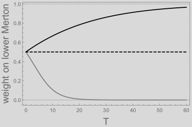
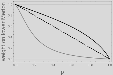
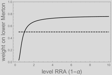
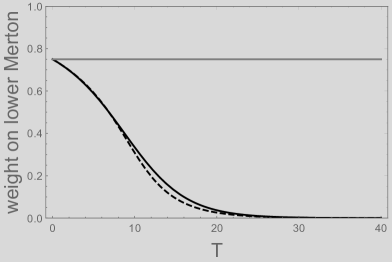
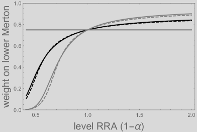
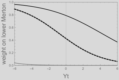
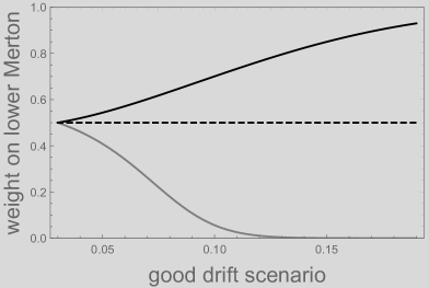
Figure 1. The figure is based on the benchmark parameter setup of Table 1 but considers the dependence on the investment horizon (upper left plot), the probability for the good drift scenario p𝑝p (upper right plot), the level of relative risk aversion 1α1𝛼1-\alpha (lower left plot), and the parameter for the good drift scenario μ¯¯𝜇\overline{\mu} (lower right plot). The plots depict the weight on the lower Merton fraction in the optimal investment strategy. In addition, each figure contains the log-investor (dashed line) and the more (black line) and less (gray line) risk averse investor than the log-investor.

If u𝑢u and v𝑣v coincide, Lemma 3.3 immediately separates the impact of the inner and outer risk on the optimal investment fraction. The optimal myopic investment fraction of all investors (all levels of relative risk aversion 1α1𝛼1-\alpha), is given by the convex combination of the Merton fractions of the inner risk situations (good and bad scenario). Thus, the impact of the inner risk is simply as in the classical Merton problem while the impact of the outer risk can be stated by the weight on the good (or bad scenario). Along the lines of Lemma 3.3, the weight on the lower Merton solution (the bad scenario) is given by

1α(t,T,Y(t))=(1p)F^(t,T,Y(t))1𝛼𝑡𝑇𝑌𝑡1𝑝^𝐹𝑡𝑇𝑌𝑡\displaystyle 1-\alpha(t,T,Y(t))=(1-p)\hat{F}(t,T,Y(t))

where

F^(t,T,Y(t))^𝐹𝑡𝑇𝑌𝑡\displaystyle\hat{F}(t,T,Y(t)) :=LT(ϑ¯,z+Y(t))(F(T,z+Y(t)))γ1φTt(z)𝑑z(F(T,z+Y(t))γφTt(z)dz.\displaystyle:=\frac{\int_{\mathbb{R}}L_{T}(\underline{\vartheta},z+Y(t))(F(T,z+Y(t)))^{\gamma-1}\varphi_{T-t}(z)dz}{\int_{\mathbb{R}}(F(T,z+Y(t))^{\gamma}\varphi_{T-t}(z)dz}.

Notice that

LT(ϑ,z+Y(t))subscript𝐿𝑇italic-ϑ𝑧𝑌𝑡\displaystyle L_{T}\left(\vartheta,z+Y(t)\right) =Lt(ϑ,Y(t))LTt(ϑ,z).absentsubscript𝐿𝑡italic-ϑ𝑌𝑡subscript𝐿𝑇𝑡italic-ϑ𝑧\displaystyle=L_{t}\left(\vartheta,Y(t)\right)L_{T-t}\left(\vartheta,z\right).

This hints at two (competing) effects: one is due to learning (i.e. the observation of Y(t)𝑌𝑡Y(t) at time t𝑡t), the other effect is caused by the remaining investment horizon Tt𝑇𝑡T-t. The second effect is called time-inconsistency and vanishes for the log-investor (α0𝛼0\alpha\rightarrow 0, γ1𝛾1\gamma\rightarrow 1, respectively), i.e. F^(t,T,Y(t))=Lt(ϑ¯,Yt)F(t,Yt)^𝐹𝑡𝑇𝑌𝑡subscript𝐿𝑡¯italic-ϑsubscript𝑌𝑡𝐹𝑡subscript𝑌𝑡\hat{F}(t,T,Y(t))=\frac{L_{t}(\underline{\vartheta},Y_{t})}{F(t,Y_{t})}.555It is well understood that the problem of time inconsistency naturally arises if one aggregates utilities (cf. e.g. Desmettre and Steffensen, (2021)). We first discuss the second effect and consider the special case t=0𝑡0t=0 (Y(t)=0𝑌𝑡0Y(t)=0) where

g(α,p,T,ϑ¯,ϑ¯):=1α(0,T,0)=(1p)F^(0,T,0).assign𝑔𝛼𝑝𝑇¯italic-ϑ¯italic-ϑ1𝛼0𝑇01𝑝^𝐹0𝑇0\displaystyle g(\alpha,p,T,\underline{\vartheta},\overline{\vartheta}):=1-\alpha(0,T,0)=(1-p)\hat{F}(0,T,0).

4.1.1. Benchmark log-investor

Formally, the justification that the log-investor α0𝛼0\alpha\rightarrow 0 (with a level of relative risk aversion 1α1𝛼1-\alpha equal to 1) defines a convenient benchmark is given by Theorem 3.1 e), i.e.

limα0g(α,p,T,ϑ¯,ϑ¯)=limT0g(α,p,T,ϑ¯,ϑ¯)=1p.subscript𝛼0𝑔𝛼𝑝𝑇¯italic-ϑ¯italic-ϑsubscript𝑇0𝑔𝛼𝑝𝑇¯italic-ϑ¯italic-ϑ1𝑝\displaystyle\lim_{\alpha\rightarrow 0}g(\alpha,p,T,\underline{\vartheta},\overline{\vartheta})=\lim_{T\rightarrow 0}g(\alpha,p,T,\underline{\vartheta},\overline{\vartheta})=1-p.

Observe that the log-investor behaves in a myopic way. In the short run (T0𝑇0T\rightarrow 0), the impact of the outer risk (weight on the bad scenario/lower Merton solution) is given by the prior probability 1p1𝑝1-p. While the within regime Merton fractions depend on the individual levels of risk aversion, the myopic solution of the outer risk is risk neutral in the sense that it is given by the expected value (under the prior distribution) of the within regime Merton fractions. Obviously, for T0𝑇0T\rightarrow 0 there is no hedging demand. For the log-investor, this is also true for investment horizons T>0𝑇0T>0 (cf. Figure 1 upper left plot). In addition, the log-investor gives an important distinction: an investor who is less (more) risk averse uses a lower (higher) weight on the lower Merton fraction (bad regime), cf. Figure 1 (lower left plot).666 Rieder and Bäuerle, (2005) Theorem 9 d). Economically, this is explained by the trade-off between speculating on the better regime (and following the optimal strategy for the good regime) and hedging against the worse regime (and following the optimal strategy for the bad regime). While the log-investor acts neutral, the hedging (speculation) motive dominates for the more (less) risk averse investor.

Intuitively, the larger the difference between the two regimes, the stronger is the hedging (speculating) motive, and the more the optimal strategy moves towards the worst(best)-case strategy. An illustration is given in Figure 1 (lower right plot) which depicts the weight on the lower Merton solution for varying μ¯¯𝜇\overline{\mu}. The higher μ¯¯𝜇\overline{\mu} (the higher the difference between the regimes), the larger is the impact of the hedging (speculation) motive for the more (less) risk averse investor.

4.1.2. Long run investor

Similar reasoning applies to the investment horizon T𝑇T. The outer risk is ’higher’ for longer investment horizons. For large T𝑇T, the investor who is more risk averse than the log-investor only considers the Merton solution of the bad regime, i.e. for α<0𝛼0\alpha<0

limTg(α,p,T,ϑ¯,ϑ¯)=1.subscript𝑇𝑔𝛼𝑝𝑇¯italic-ϑ¯italic-ϑ1\displaystyle\lim_{T\rightarrow\infty}g(\alpha,p,T,\underline{\vartheta},\overline{\vartheta})=1.

Thus, w.r.t. the outer risk, the long term investor who is more risk averse than the log-investor acts extremely risk averse. In contrast, a long term investor who is less risk averse than the log-investor only considers the good regime.777 Bäuerle and Grether, (2017) Theorem 3.1, Theorem 3.3 In consequence, for long term investment horizons (T𝑇T\rightarrow\infty), the prior distribution has no impact on the weight α(0,T,y)𝛼0𝑇𝑦\alpha(0,T,y), i.e. α(0,T,y)=0𝛼0𝑇𝑦0\alpha(0,T,y)=0 (α(0,T,y)=1𝛼0𝑇𝑦1\alpha(0,T,y)=1) for α<0𝛼0\alpha<0 (for α>0𝛼0\alpha>0). The long term investor only considers the worst (best) case drift, i.e. μ¯¯𝜇\underline{\mu} (μ¯¯𝜇\overline{\mu}) and behaves along the lines of a maximin (maximax) decision rule. This is further emphasized by means of the sensitivities of the optimal weight on the lower Merton investment fraction. An illustration is given by Figure 1 (upper left plot) which depicts the weight on the lower Merton fraction for varying investment horizons T𝑇T. See also subsections 4.1.4, 4.1.5.

4.1.3. Impact of prior distribution

Difference to log-investor (g(α,p,T,ϑ¯,ϑ¯)(1p)𝑔𝛼𝑝𝑇¯italic-ϑ¯italic-ϑ1𝑝g(\alpha,p,T,\underline{\vartheta},\overline{\vartheta})-(1-p))

Refer to caption
Refer to caption
Refer to caption
Refer to caption
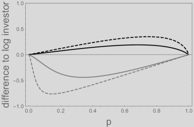
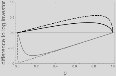
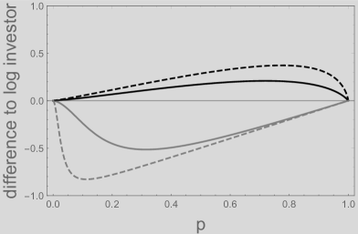
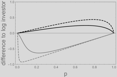
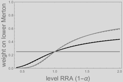
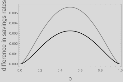
Figure 2. If not otherwise mentioned below, the figure refers to the benchmark parameter scenario of Table 1. The figure compares, for varying priors p𝑝p, the weight on the lower Merton fraction to the one of the log-investor, i.e. it depicts the difference g(α,p,T,ϑ¯,ϑ¯)(1p)𝑔𝛼𝑝𝑇¯italic-ϑ¯italic-ϑ1𝑝g(\alpha,p,T,\underline{\vartheta},\overline{\vartheta})-(1-p). The black (gray) lines refer to the investor who is more (less) risk averse than the log-investor. The investment horizon is T=10𝑇10T=10 (thick lines) and T=20𝑇20T=20 (dashed lines). The upper right figure is then based on μ¯=0.12¯𝜇0.12\overline{\mu}=0.12 (instead of the benchmark parameter μ¯=0.09¯𝜇0.09\overline{\mu}=0.09). The lower left plot then considers the benchmark scenario with the exception that μ¯=0.01¯𝜇0.01\underline{\mu}=0.01 (instead of μ¯=0.03¯𝜇0.03\underline{\mu}=0.03). The last figure (lower right plot) considers a higher risk aversion (α=2𝛼2\alpha=-2 instead of α=1𝛼1\alpha=-1) for the black lines and a lower risk aversion (α=0.6𝛼0.6\alpha=0.6 instead of α=0.5𝛼0.5\alpha=0.5) for the gray lines.

Intuitively, the weight on the lower Merton investment fraction is decreasing (increasing) in the prior probability p𝑝p (1p1𝑝1-p) (upper right plot of Figure 1). This is obvious for the log-investor who simply relies on the prior probability. However, notice again the important distinction based on the benchmark log-investor. While the more risk averse investor (black line) uses a higher weight on the lower Merton solution, the opposite is true for the less risk averse investor (gray line). Intuitively, the discrepancy is the highest for some intermediate p𝑝p. While there is no outer risk implied in the extreme cases that p0𝑝0p\rightarrow 0 or p1𝑝1p\rightarrow 1, the outer risk is ’maximal’ for some intermediate p𝑝p (which depends on the investment horizon T𝑇T, the level of relative risk aversion 1α1𝛼1-\alpha, and the relation between good and bad scenario). The outer risk situation also increases in the distance between the good and bad regime (μ¯¯𝜇\overline{\mu} and μ¯¯𝜇\underline{\mu}). Thus, the deviation of a more (less) risk averse investor from the log-investor is the higher, the higher the distance is, e.g. it is increasing in μ¯¯𝜇\overline{\mu} (cf lower right figure of Figure 1). An additional illustration is given by Figure 2 which depicts the difference to the log-investor by means of

g(α,p,T,ϑ¯,ϑ¯)(1p),𝑔𝛼𝑝𝑇¯italic-ϑ¯italic-ϑ1𝑝g(\alpha,p,T,\underline{\vartheta},\overline{\vartheta})-(1-p),

i.e. the difference of the weight on the lower Merton solution and 1p1𝑝1-p which is the weight of the log-investor. All figures include two investment horizons (T=10𝑇10T=10 and T=20𝑇20T=20). Observe that the deviation from the log-investor is the higher, the higher the investment horizon is. For the investor who is more (less) risk averse than the log-investor, the highest deviation is obtained for p>0.5𝑝0.5p>0.5 (p<0.5𝑝0.5p<0.5). Recall that the more (less) risk averse investor tends to hedge (speculate) the bad (good) drift scenario. In consequence, the prior probability p𝑝p with the highest deviation increases (decreases) in the investment horizon. Analogous reasoning is true w.r.t. the sensitivity to μ¯¯𝜇\overline{\mu} (μ¯¯𝜇\underline{\mu}) and the level of risk aversion 1α1𝛼1-\alpha (cf. Figure 2).

4.1.4. Learning vs. pre-commitment

Comparison of optimal initial learning and pre-commitment strategy
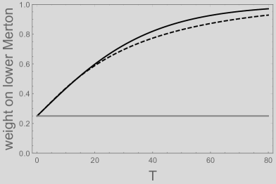
Refer to caption
Refer to caption
Refer to caption
Refer to caption
Figure 3. If not otherwise mentioned below, the figure refers to the benchmark parameter scenario of Table 1. The upper plots are based on p=0.75𝑝0.75p=0.75 (i.e. 1p=0.251𝑝0.251-p=0.25) while the lower plots refer to p=0.25𝑝0.25p=0.25 (i.e. 1p=0.751𝑝0.751-p=0.75). The left hand figures compare the optimal weight on the lower Merton solution of the learning (black) and pre-commitment setup (dashed) for varying investment horizons T𝑇T. The upper (lower) figure concerns the investor who is more (less) risk averse than the log-investor. The right hand figures depict, for T=10𝑇10T=10 (black) and T=20𝑇20T=20 (gray), the weight on the lower Merton solution for varying levels of relative risk aversion. Again, the black lines refer to strategies under learning while the dashed ones are pre-commitment strategies.

It is worth to mention that similar reasoning as above is valid in a pre-commitment setup (cf. optimization problem (3.4)). First notice that, in the classical Bayesian setup, the optimal investment fraction of the log-investor does not depend on T𝑇T. Thus, the optimal pre-commitment and learning strategies coincide at t=0𝑡0t=0. In addition, this is true for the limiting cases of a myopic investor (T0𝑇0T\rightarrow 0) and the long term investor (T𝑇T\rightarrow\infty). For an investor who is more risk averse than the log-investor, recall now the hedging motive. W.r.t. the trade-off between speculating on the better regime (and following the optimal strategy for the good regime) and hedging against the worse regime (and following the optimal strategy for the bad regime), the hedging motive dominates. In addition, observe that the hedging motive is increasing in the investment horizon T𝑇T. Compared to the setup under learning, pre-commitment implies that the investor must pre-commit to a constant investment fraction at t=0𝑡0t=0. In the optimum, she anticipates that gradually over time, the remaining investment horizon decreases. Therefore, at t=0𝑡0t=0, the hedging demand is, for rather high investment horizons T𝑇T, lower in the pre-commitment setup than under learning. The above reasoning is illustrated in Figure 3. The left figure compares (for an investor who is more risk averse than the log-investor) the optimal weight on the lower Merton solution of the learning (black) and pre-commitment setup (dashed) for varying investment horizons T𝑇T. Observe that the strategies coincide in the limiting cases. In addition, for intermediate investment horizons T𝑇T, the pre-commitment strategy has a lower weight on the bad scenario (lower Merton solution). This implies that (at t=0𝑡0t=0) the pre-commitment strategy is more aggressive than the learning strategy. As mentioned above, this is due to the fact that the investor who must pre-commit already has to anticipate that, in the future, the remaining investment horizon is lower which is associated with a lower hedging demand (against the bad scenario). The right plot of Figure 3 depicts the weight on the lower Merton solution for varying levels of relative risk aversion. Again, the black line refers to learning while the dashed one is pre-commitment. Observe that the strategies (the weights on the lower Merton solution) coincide in the case of a log-investor (α0𝛼0\alpha\rightarrow 0) with level of relative risk aversion equal to one. Overall, however, our numerical results do not show a very big difference between the pre-commitment and the learning strategy.

4.1.5. Value of learning and impact of investment horizon

An intuitive explanation for the similarity of learning and pre-commitment at t=0𝑡0t=0 is given by means of the conditional distribution of ϑitalic-ϑ\vartheta. Along the lines of Remark 2.2, it holds

P(Θ=ϑ¯|Y(t))𝑃Θconditional¯italic-ϑsuperscript𝑌𝑡\displaystyle P\left(\left.\Theta=\overline{\vartheta}\right|\mathcal{F}^{Y}(t)\right) =pL(ϑ¯,Y(t))F(t,Y(t))=:p^t and P(Θ=ϑ¯|Y(t))=1p^t\displaystyle=p\frac{L(\overline{\vartheta},Y(t))}{F(t,Y(t))}=:\hat{p}_{t}\text{ and }P\left(\left.\Theta=\underline{\vartheta}\right|\mathcal{F}^{Y}(t)\right)=1-\hat{p}_{t}

such that Θ^(t)=E[Θ|Y(t)]=p^tϑ¯+(1p^t)ϑ¯^Θ𝑡𝐸delimited-[]conditionalΘsuperscript𝑌𝑡subscript^𝑝𝑡¯italic-ϑ1subscript^𝑝𝑡¯italic-ϑ\hat{\Theta}(t)=E\left[\left.\Theta\right|\mathcal{F}^{Y}(t)\right]=\hat{p}_{t}\overline{\vartheta}+(1-\hat{p}_{t})\underline{\vartheta}. Recall that, at t=0𝑡0t=0, the investor maximizes her expected utility under the prior distribution. Thus, the optimal strategy depends on the expected value of Θ^(t)^Θ𝑡\hat{\Theta}(t) which is

𝔼[Θ^(t)]𝔼delimited-[]^Θ𝑡\displaystyle\mathbb{E}\left[\hat{\Theta}(t)\right] =pϑ¯+(1p)ϑ¯absent𝑝¯italic-ϑ1𝑝¯italic-ϑ\displaystyle=p\overline{\vartheta}+(1-p)\underline{\vartheta}

by the martingale property of Θ^^Θ\hat{\Theta}. This is the same for a pre-commitment and a learning investor.

In summary, at t=0𝑡0t=0, both (pre-commitment and learning) have the same information and the investor only expects to learn the prior distribution such that for the log-investor there is no difference between the pre-commitment and learning strategy (cf. Remark 2.2), and a negligible difference for an investor with α0𝛼0\alpha\neq 0.

However, the evolutions of the strategies under learning and pre-commitment are rather different. While the pre-commitment investment fraction is (per definition) constant over time, the time t𝑡t investment fraction under learning is a random variable defined by Y(t)𝑌𝑡Y(t). Notice that in our stylized illustration the true model is either given in terms of ϑ=ϑ¯italic-ϑ¯italic-ϑ\vartheta=\overline{\vartheta} (Model 1 where Y(t)N(ϑ¯t,t)similar-to𝑌𝑡𝑁¯italic-ϑ𝑡𝑡Y(t)\sim N\left(\overline{\vartheta}t,t\right)) or ϑ=ϑ¯italic-ϑ¯italic-ϑ\vartheta=\underline{\vartheta} (Model 2 where Y(t)N(ϑ¯t,t)similar-to𝑌𝑡𝑁¯italic-ϑ𝑡𝑡Y(t)\sim N\left(\underline{\vartheta}t,t\right)) such that we can compare the conditional distributions of the investment fraction, i.e. given Model 1 and Model 2. In order to focus on the impact of learning, consider the log-investor whose strategy is exclusively specified in terms of p^tsubscript^𝑝𝑡\hat{p}_{t}. Straightforward calculations imply that with ZN(0,1)similar-tosuperscript𝑍𝑁01Z^{*}\sim N(0,1) it holds

p^t|Model 1evaluated-atsubscript^𝑝𝑡Model 1\displaystyle\left.\hat{p}_{t}\right|_{\text{Model 1}} (1+qLt(ϑ¯ϑ¯,tZ))1similar-toabsentsuperscript1𝑞subscript𝐿𝑡¯italic-ϑ¯italic-ϑ𝑡superscript𝑍1\displaystyle\sim\left(1+q\;L_{t}(\underline{\vartheta}-\overline{\vartheta},\sqrt{t}Z^{*})\right)^{-1}
p^t|Model 2evaluated-atsubscript^𝑝𝑡Model 2\displaystyle\left.\hat{p}_{t}\right|_{\text{Model 2}} (1+qexp{(ϑ¯ϑ¯)2t}Lt(ϑ¯ϑ¯,tZ))1similar-toabsentsuperscript1𝑞superscript¯italic-ϑ¯italic-ϑ2𝑡subscript𝐿𝑡¯italic-ϑ¯italic-ϑ𝑡superscript𝑍1\displaystyle\sim\left(1+q\exp\{(\underline{\vartheta}-\overline{\vartheta})^{2}t\}\;L_{t}(\underline{\vartheta}-\overline{\vartheta},\sqrt{t}Z^{*})\right)^{-1}

Conditional distribution of p^tsubscript^𝑝𝑡\hat{p}_{t}

Refer to caption
Refer to caption
Refer to caption
Refer to caption
Figure 4. The figure illustrates the conditional distribution of p^tsubscript^𝑝𝑡\hat{p}_{t} given Model 1 (black) and Model 2 (gray). It is based on the benchmark model parameter setup of Table 1. The left (right) hand plots refer to t=5𝑡5t=5 (t=10𝑡10t=10). For the upper (lower) plots it holds p=0.5𝑝0.5p=0.5 (p=0.75𝑝0.75p=0.75.)

An illustration of the conditional distributions is given in Figure 4. Notice that comparing the densities in the first row at time points t=5𝑡5t=5 (left) and t=10𝑡10t=10 (right) that the true model is learned by the density. Indeed, at time point t=10𝑡10t=10 depending on what has been observed, the investment strategies will be quite different. However, the second row of pictures shows that learning may be slow when the initial prior is mainly wrong. Then the probability mass shifts rather slowly to the correct model.

However, a pure learning effect is only immanent in the strategy of the log-investor. Any deviation from the log-investor gives, in addition, rise to a competing effect caused by the dependence of the remaining investment horizon Tt𝑇𝑡T-t. This is illustrated in Figure 5 which depicts the weight on the lower Merton solution for varying observations of Y(t)𝑌𝑡Y(t). Obviously, the weight on the lower Merton solution is decreasing in Y(t)𝑌𝑡Y(t), i.e. a higher observation is in favour of Model 1 (where ϑ=ϑ¯italic-ϑ¯italic-ϑ\vartheta=\overline{\vartheta}). While the weights of the log investor (dashed lines) do not depend on the remaining investment horizon Tt𝑇𝑡T-t (upper plots versus lower plots), the horizon effect for an investor who deviates from the log-investor implies that the dependence of the weight on Y(t)𝑌𝑡Y(t) vanishes for increasing Tt𝑇𝑡T-t, i.e. the more (black line) and less (gray line) risk averse investor moves to the lower (upper) Merton solution.

Weight on lower Merton solution for varying Ytsubscript𝑌𝑡Y_{t}
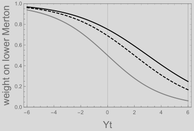
Refer to caption
Refer to caption
Refer to caption
Refer to caption
Figure 5. The figures illustrate the weight on the lower Merton solution at time t𝑡t and an investment horizon T𝑇T for varying Ytsubscript𝑌𝑡Y_{t}. Each figure contains the log-investor (dashed line) and the more (black line) and less (gray line) risk averse investor than the log-investor. It is based on the benchmark model parameter setup of Table 1. The upper (lower) plots refer to t=5𝑡5t=5 and T=10𝑇10T=10 (T=30𝑇30T=30). For the left (right) plots it holds p=0.5𝑝0.5p=0.5 (p=0.75𝑝0.75p=0.75.)

To assess the value of learning, we have to compare the expected utilities (certainty equivalents) of the optimal strategy under learning versus pre-commitment. For a pure value of learning, we consider the log-investor. Notice that the expected utility v𝑣v of the optimal strategy is (for x0=1subscript𝑥01x_{0}=1) given by

v(x0)𝑣subscript𝑥0\displaystyle v(x_{0}) =F(T,z)lnF(T,z)φT(z)𝑑z.absentsubscript𝐹𝑇𝑧𝐹𝑇𝑧subscript𝜑𝑇𝑧differential-d𝑧\displaystyle=\int_{\mathbb{R}}F(T,z)\ln F(T,z)\varphi_{T}(z)dz.

In contrast, the value of the optimal pre-commitment strategy is

vpre(x0)superscript𝑣presubscript𝑥0\displaystyle v^{\text{pre}}(x_{0}) =(pμ¯+(1p)μ¯)22σ2T.absentsuperscript𝑝¯𝜇1𝑝¯𝜇22superscript𝜎2𝑇\displaystyle=\frac{(p\overline{\mu}+(1-p)\underline{\mu})^{2}}{2\sigma^{2}}T.

For the log-investor, the value of learning in terms of the savings rate difference which is here given by

1T(v(x0)vpre(x0))1𝑇𝑣subscript𝑥0superscript𝑣presubscript𝑥0\displaystyle\frac{1}{T}(v(x_{0})-v^{\text{pre}}(x_{0}))

is illustrated by means of Figure 6. Here, the value of learning is increasing in T𝑇T (cf. left hand figure). Obviously, the value of learning is zero in the degenerate cases that p=0𝑝0p=0 (p=1𝑝1p=1, respectively) and obtains its maximum value approximately for p=0.5𝑝0.5p=0.5 (cf. right hand figure).

Value of learning
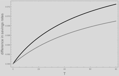
Refer to caption
Refer to caption
Figure 6. The figures illustrate the value of learning in terms of the savings rate difference (learning versus pre-commitment). It is based on the benchmark model parameter setup of Table 1 and p=0.5𝑝0.5p=0.5 (black), p=0.75𝑝0.75p=0.75 (gray) in the left plot, T=10𝑇10T=10 (black), T=20𝑇20T=20 (gray) in the right plot.

4.1.6. Impact of good drift scenario and volatility on investment fraction.

The previous sensitivities mainly referred to the outer risk parameters p𝑝p and T𝑇T. We now consider the sensitivities of the inner risk parameters μ¯¯𝜇\overline{\mu} and σ𝜎\sigma. While the outer risk parameters have no impact on the inner risk situation, the model parameters μ¯¯𝜇\overline{\mu} and σ𝜎\sigma give rise to an inner and outer effect. Thus, we have to discuss the combined effects on the optimal investment fraction κ(t,T,Y(t))𝜅𝑡𝑇𝑌𝑡\kappa(t,T,Y(t)). To simplify the exposition, we only consider the case of a more risk averse investor than the log-investor along with our benchmark parameters and t=0,Y(t)=0formulae-sequence𝑡0𝑌𝑡0t=0,Y(t)=0.

First consider the drift parameter of the good scenario μ¯¯𝜇\overline{\mu}. The inner risk effect concerns the Merton fraction in the good scenario which is linearly increasing in μ¯¯𝜇\overline{\mu} while there is no impact on the lower Merton fraction. The directional effect on the investment fraction κ𝜅\kappa is positive. However, the outer risk effect is captured by the hedging motive. Recall (cf. Figure 1 and its explanation) that the higher μ¯¯𝜇\overline{\mu} (the higher the difference between the regimes), the larger is the impact of the hedging motive for the more (than log) risk averse investor. The higher μ¯¯𝜇\overline{\mu}, the higher is the weight on the lower Merton solution which decreases the investment fraction κ𝜅\kappa. In summary, there are opposing effects.

Now, consider the volatility σ𝜎\sigma. Notice that the volatility is a scaling factor to the Merton fractions. The higher the volatility is, the lower are both, the upper and lower Merton fraction, i.e. the inner risk effect to the investment fraction κ𝜅\kappa is negative. In contrast, the outer risk effect is positive, i.e. a higher volatility decreases the difference between good and bad scenario (in terms of the market price per unit of risk or, alternatively, the Merton fractions of the inner risk situation) which reduces the hedging motive. Intuitively, the inner effect is the dominating one since κ𝜅\kappa is given in terms of a weighted average of upper and lower Merton fraction.

Impact of μ¯¯𝜇\overline{\mu} and σ𝜎\sigma

Refer to caption
Refer to caption
Refer to caption
Refer to caption
Figure 7. The figure depicts the impact of varying μ¯¯𝜇\overline{\mu} (upper plots) and varying σ𝜎\sigma (lower plots) on the investment fraction κsuperscript𝜅\kappa^{*}. It is based on the benchmark model parameter setup of Table 1 with the exception that the level of relative risk aversion is equal to 4 (α=3𝛼3\alpha=-3). While the black lines refer to p=0.5𝑝0.5p=0.5 (benchmark), the gray (dotted) lines are based on p=0.25𝑝0.25p=0.25 (p=0.75𝑝0.75p=0.75). In addition, the left (right) plots refer to T=10𝑇10T=10 (T=20𝑇20T=20).

An illustration is given by means of Figure 7. It depicts the impact of varying μ¯¯𝜇\overline{\mu} (upper plots) and varying σ𝜎\sigma (lower plots) on the investment fraction κ𝜅\kappa. Observe that, in spite of the opposing effects, the optimal investment fraction κ𝜅\kappa is decreasing in σ𝜎\sigma. However, varying only the upper drift μ¯¯𝜇\overline{\mu} emphasizes the opposing effects. The investment fraction is first increasing (i.e. the inner risk impact is dominating) while, after a critical drift level, it is decreasing (i.e. the hedging motive is dominating). In addition, observe that the critical level is decreasing in T𝑇T. Finally, it is also worth to emphasize that the inner risk parameters have a crucial impact on learning. Notice that Ytsubscript𝑌𝑡Y_{t} depends on both, μ¯¯𝜇\overline{\mu} and σ𝜎\sigma.

4.2. Impact of ambiguity

Throughout the following, we assume that the investor is more risk averse than the log-investor, i.e. α<0𝛼0\alpha<0. Notice that the investor is risk averse if and only if u𝑢u is concave, while she is ambiguity averse if and only if v𝑣v is a concave transformation of u𝑢u. Assuming that u𝑢u and v𝑣v are CRRA functions with relative risk (ambiguity) aversion 1α1𝛼1-\alpha (1λ1𝜆1-\lambda) implies that an ambiguity neutral investor is characterized by λ=α𝜆𝛼\lambda=\alpha while she is ambiguity averse (loving) for λ<α<0𝜆𝛼0\lambda<\alpha<0 ( 0>λ>α0𝜆𝛼0>\lambda>\alpha).

Again, we consider the impact of the outer risk (evaluated by the ambiguity function v𝑣v) by means of the weight on the lower (upper) Merton solution (implied by the utility function u𝑢u), i.e. we are interested in g(α,pmod,)𝑔𝛼superscript𝑝modg(\alpha,p^{\text{mod}},\dots) where

pmod:=q1/(q1+q2)assignsuperscript𝑝modsuperscriptsubscript𝑞1superscriptsubscript𝑞1superscriptsubscript𝑞2p^{\text{mod}}:=q_{1}^{*}/(q_{1}^{*}+q_{2}^{*})

(cf. Lemma 3.4, 3.6 and 3.8). We call pmodsuperscript𝑝modp^{\text{mod}} the adjusted or modified probability. The ambiguity neutral investor serves as a benchmark since pmod=psuperscript𝑝mod𝑝p^{\text{mod}}=p, i.e. the modified probability coincides with the prior probability.

Recall (cf. Subsection 4.1.3) that the weight on the lower Merton solution is decreasing in the prior probability p𝑝p. Thus, introducing ambiguity aversion (loving) is equivalent to decreasing (increasing) the prior probability p𝑝p for the good drift scenario. Assume now that both, the level of risk aversion and ambiguity aversion are above the one of the benchmark log-investor, i.e. α<0𝛼0\alpha<0 and λ<0𝜆0\lambda<0. Recall that we already discussed the special case λ=α𝜆𝛼\lambda=\alpha in Subsection 4.1. Intuitively, the investor chooses less risk (a higher weight on the lower Merton solution) under ambiguity aversion, i.e. if the relative ambiguity aversion is higher than the level of risk aversion, i.e. if λ<α𝜆𝛼\lambda<\alpha (1λ>1α1𝜆1𝛼1-\lambda>1-\alpha). In terms of the probability adjustment this implies that the modified probability pmodsuperscript𝑝modp^{\text{mod}} is smaller than p𝑝p, i.e. the investor is characterized by a lower weight on the upper Merton solution than the ambiguity neutral investor. In contrast, if λ>α𝜆𝛼\lambda>\alpha (1λ<1α1𝜆1𝛼1-\lambda<1-\alpha) implies that pmodsuperscript𝑝modp^{\text{mod}} is higher than p𝑝p. A numerical illustration of the modified probability is given in Figure 8 (left plot). The level of relative risk aversion is 1α=41𝛼41-\alpha=4. Notice that the modified prior probability pmodsuperscript𝑝modp^{\text{mod}} is decreasing in the level of relative ambiguity aversion 1λ1𝜆1-\lambda and tends to zero for 1λ1𝜆1-\lambda\to\infty. Mathematically this is clear since the smaller of the two values in (3.5) (note λ<0𝜆0\lambda<0) dominates the optimization problem. From an economic point of view the very ambiguity averse investor tries to maximize her worst-case utility. In particular, it is above (below) the prior p𝑝p in the case that 1λ<1α1𝜆1𝛼1-\lambda<1-\alpha (1λ>1α1𝜆1𝛼1-\lambda>1-\alpha). Notice that the effect is more pronounced for higher times to maturity T𝑇T, i.e. the impact on the modified prior probability is increasing in T𝑇T. However, recall that the impact of the prior probability is decreasing in T𝑇T, i.e. for T𝑇T\rightarrow\infty the (more than log) risk averse investor only relies on the worst drift scenario. Hence the effect of ambiguity aversion is fading for large time horizons. This is natural, since a large time horizon allows for perfectly learning the model. For T0𝑇0T\to 0 the modified prior tends to the initial given prior. This is because for a very short time horizon there is almost no difference between the two scenarios. However, recall that pmodsuperscript𝑝𝑚𝑜𝑑p^{mod} depends on both, time horizon and ambiguity aversion. Thus, in the end the combination of both effects is crucial. The overall effect on the investment fraction (represented by the weight on the lower Merton solution) is smooth (cf. Figure 8 (right plot)).

Impact of ambiguity aversion on modified probability pmodsuperscript𝑝modp^{\text{mod}} and weight on lower Merton solution

Refer to caption
Refer to caption
Figure 8. Model parameters are given as before (cf. Table 1). The prior probability for the good drift scenario is p=0.5𝑝0.5p=0.5, the level of relative risk aversion is equal to 4 (1α=41𝛼41-\alpha=4). The figure on the left hand side depicts the modified prior probability for varying levels of relative ambiguity aversion 1λ1𝜆1-\lambda. The figure on the right hand side gives the corresponding weights on the lower Merton solution. The black lines refers to an investment horizon of T=10𝑇10T=10 years, the dashed one to T=20𝑇20T=20, and the gray one to T=50𝑇50T=50.

4.3. Comments on implementation and practical relevance

We give some brief comments on the practical relevance of the derived strategies w.r.t.  their implementation on historical return data, the possibilities to test the out-of-sample performance and the complexity caused by these problems. Since the objective to maximize the expected value (w.r.t. different drift scenarios) of the expected utility of an investor with constant relative risk aversion is motivated by estimation risk, we also refer to other approaches which deal with estimation risk and some empirical results.

In the first instance, it is convenient to consider the problem in the classic mean variance setup. The discrete time version of the price dynamics of the risky assets S1,,Sdsubscript𝑆1subscript𝑆𝑑S_{1},\dots,S_{d} has returns rit=SitSi,t11subscript𝑟𝑖𝑡subscript𝑆𝑖𝑡subscript𝑆𝑖𝑡11r_{it}=\frac{S_{it}}{S_{i,t-1}}-1 and log returns ln(1+rit)rit1subscript𝑟𝑖𝑡subscript𝑟𝑖𝑡\ln(1+r_{it})\approx r_{it}. Let rftsubscript𝑟𝑓𝑡r_{ft} denote the return of the risk free asset, the excess return is defined by Rt:=rtrft1dassignsubscript𝑅𝑡subscript𝑟𝑡subscript𝑟𝑓𝑡subscript1𝑑R_{t}:=r_{t}-r_{ft}1_{d} where 1dsubscript1𝑑1_{d} is an d𝑑d-vector of ones. It is assumed that Rtsubscript𝑅𝑡R_{t} follows a multivariate normal distribution with mean μ𝜇\mu and covariance matrix ΣΣ\Sigma. For portfolio weights κ𝜅\kappa (for the risky assets) the objective function of a short-term expected utility maximizing investor with constant relative risk aversion is, in the above context, equivalent to the mean-variance objective function

U(κ)=μPF1α2(σPF)2=μPF12γ(σPF)2𝑈𝜅superscript𝜇PF1𝛼2superscriptsuperscript𝜎PF2superscript𝜇PF12𝛾superscriptsuperscript𝜎PF2\displaystyle U(\kappa)=\mu^{\text{PF}}-\frac{1-\alpha}{2}\left(\sigma^{\text{PF}}\right)^{2}=\mu^{\text{PF}}-\frac{1}{2\gamma}\left(\sigma^{\text{PF}}\right)^{2}

where 1α=1γ1𝛼1𝛾1-\alpha=\frac{1}{\gamma} denotes the level of relative risk aversion, μPF=κμsuperscript𝜇𝑃𝐹superscript𝜅𝜇\mu^{PF}=\kappa^{\prime}\mu the portfolio mean, and (σPF)2=κΣ1κsuperscriptsuperscript𝜎PF2superscript𝜅superscriptΣ1𝜅\left(\sigma^{\text{PF}}\right)^{2}=\kappa^{\prime}\Sigma^{-1}\kappa the portfolio variance. For known μ𝜇\mu and ΣΣ\Sigma, the optimal portfolio weights are

κ=11αΣ1μ=γ(σT)1ϑ=:κMer(γ,ϑ)\displaystyle\kappa^{*}=\frac{1}{1-\alpha}\Sigma^{-1}\mu=\gamma(\sigma^{T})^{-1}\vartheta=:\kappa^{\text{Mer}}(\gamma,\vartheta)

Since the true model parameters μ𝜇\mu (and ΣΣ\Sigma) are not known, it is not possible to implement the optimal investment fraction κsuperscript𝜅\kappa^{*}. A naive way to solve the problem is the so called plug-in rule where the investor relies on the sample estimates of N𝑁N periods of observed returns (training data) and treats them as true parameters.

Along the lines of Kan and Zhou, (2007), a portfolio rule κ^^𝜅\hat{\kappa} is defined by a function f𝑓f of the training data R1,,RNsubscript𝑅1subscript𝑅𝑁R_{1},\dots,R_{N} and the out-of-sample performance of a portfolio rule can be measured by the expected utility U~~𝑈\tilde{U} conditional on the weights being chosen by κ^^𝜅\hat{\kappa}. In particular, they consider the loss by means of the difference U(κ)E[U~(κ^)]𝑈superscript𝜅𝐸delimited-[]~𝑈^𝜅U(\kappa^{*})-E[\tilde{U}(\hat{\kappa})]. Kan and Zhou, (2007) analytically derive the expected loss function for the (naive) plug-in approach and show that this approach can lead to very poor out-of-sample performance.

To implement our (dynamic) strategy (which includes learning), we need a prior distribution for μ𝜇\mu. Thus, it is, in the first instance necessary to determine a suitable estimator for the prior distribution (cf. e.g. Bauder et al., (2021)). An interesting question is whether it is possible to reduce the problem to a two point prior without causing too much sub-optimality (in particular, w.r.t the dynamic version of the strategy). In addition, the implementation of the strategy affords an estimator for the covariance matrix ΣΣ\Sigma (where σT=σ1Σsuperscript𝜎𝑇superscript𝜎1Σ\sigma^{T}=\sigma^{-1}\Sigma). For example, Ledoit and Wolf, (2017) promote a nonlinear shrinkage estimator and show that their estimator dominates its competitors on historical stock returns data.

S&P500 index value and daily returns
Refer to caption
Refer to caption
Figure 9. S&P500 price path and daily returns from 2010.01.012010.01.012010.01.01 to 2024.01.012024.01.012024.01.01.

Comparison of strategies for volatility windows (250 versus 50 days)
Refer to caption
Refer to caption
Refer to caption
Refer to caption
Refer to caption
Refer to caption
Figure 10. The figure depicts the historical volatilities of the S&P500 index for a rolling window of 250 and 50 trading dates (upper plots). Scaling the daily S&P500 index returns with the historical volatilities then gives the daily increments of YtYt1subscript𝑌𝑡subscript𝑌𝑡1Y_{t}-Y_{t-1} where Y(0)=0𝑌00Y(0)=0. The plots in the middle illustrate Y(t)𝑌𝑡Y(t) based on the volatility estimates resulting from a window of the prior 250 (left hand plot) and 50 (right hand plot) trading dates. The lower plots then depict the investment fractions of an investor with a level of relative risk aversion of 6 (α=5𝛼5\alpha=-5) (and T=14𝑇14T=14 years) who relies on μ¯=0.09¯𝜇0.09\overline{\mu}=0.09 and μ¯=0.03¯𝜇0.03\underline{\mu}=0.03 with a prior probability p=0.5𝑝0.5p=0.5 (black line). The learning strategy κ𝜅\kappa is compared to a naive investor who uses μ¯=μ¯=0.9¯𝜇¯𝜇0.9\overline{\mu}=\underline{\mu}=0.9 (dashed gray) and one with μ¯=μ¯=0.3¯𝜇¯𝜇0.3\overline{\mu}=\underline{\mu}=0.3 (gray).

Comparison of Bayesian strategies (different (μ¯,μ¯)¯𝜇¯𝜇(\overline{\mu},\underline{\mu}) and p𝑝p)

Refer to caption
Refer to caption
Figure 11. The figure illustrates variations of the investment fraction of the benchmark investor ((μ¯,μ¯)=(0.09;0.03)¯𝜇¯𝜇0.090.03(\overline{\mu},\underline{\mu})=(0.09;0.03) and p=0.5𝑝0.5p=0.5) considered in Figure 10. The benchmark is indicated by the black line. In the left plot, the gray (dashed) line is implied by (μ¯,μ¯)=(0.1;0.01)¯𝜇¯𝜇0.10.01(\overline{\mu},\underline{\mu})=(0.1;0.01) ( (μ¯,μ¯)=(0.06;0.02)¯𝜇¯𝜇0.060.02(\overline{\mu},\underline{\mu})=(0.06;0.02)). The right plot uses modified a priori probabilities, i.e. p=0.25𝑝0.25p=0.25 (gray line) and p=0.75𝑝0.75p=0.75 (dashed line).

Once Σ^^Σ\hat{\Sigma} and the prior distribution of μ𝜇\mu are calculated by means of the training data, the investor can initialize the strategy with Y(0)=0𝑌00Y(0)=0. Afterwards (at time t𝑡t), it is necessary to plug-in the observed cummulated increments Yt1+ΔY^tsubscript𝑌𝑡1Δsubscript^𝑌𝑡Y_{t-1}+\Delta\hat{Y}_{t}. Notice that the increments are based on the estimate σ^^𝜎\hat{\sigma} (the estimated covariance matrix Σ^^Σ\hat{\Sigma}, respectively). Thus, a practical application may also reconsider the estimated covariance matrix Σ^^Σ\hat{\Sigma} and the possible (two point) values of μ𝜇\mu.

To get some further intuition about the implementation and the problems herein, consider e.g. the case of one risky asset where St=S0exp(σWt+μt12σ2t)=S0exp(σYt12σ2t)subscript𝑆𝑡subscript𝑆0𝜎subscript𝑊𝑡𝜇𝑡12superscript𝜎2𝑡subscript𝑆0𝜎subscript𝑌𝑡12superscript𝜎2𝑡S_{t}=S_{0}\exp(\sigma W_{t}+\mu t-\frac{1}{2}\sigma^{2}t)=S_{0}\exp(\sigma Y_{t}-\frac{1}{2}\sigma^{2}t) such that

YtYt1=1σln(St/St1)+12σ1σ(St/St11)+12σsubscript𝑌𝑡subscript𝑌𝑡11𝜎subscript𝑆𝑡subscript𝑆𝑡112𝜎1𝜎subscript𝑆𝑡subscript𝑆𝑡1112𝜎Y_{t}-Y_{t-1}=\frac{1}{\sigma}\ln(S_{t}/S_{t-1})+\frac{1}{2}\sigma\approx\frac{1}{\sigma}(S_{t}/S_{t-1}-1)+\frac{1}{2}\sigma

For a given (discounted) price path of the risky asset (e.g. with daily observations), a naive way is to plug for σ^^𝜎\hat{\sigma} the historical volatility of the price path over a rolling window of prior trading dates. To illustrate the implementation, assume that the (discounted) price path of the risky asset is given by the S&P500 index values from 2010.01.012010.01.012010.01.01 to 2024.01.012024.01.012024.01.01 (cf. Figure 9). The upper plots of Figure 10 illustrate the corresponding historical volatilities based on the last 250 (and 50) trading dates. The resulting Y𝑌Y pathes are depicted in the middle plots. It is worth to emphasize that the asset price path (S&P500 index path) is one realization of the true data generating process such that the corresponding path of Y𝑌Y only depends on the volatility estimator. Now consider the path of the investment fraction κ𝜅\kappa of an Bayesian investor with constant relative risk aversion 1α=61𝛼61-\alpha=6 and an investment horizon of T=14𝑇14T=14 years. In addition to Y(t)𝑌𝑡Y(t), her investment fraction depends on her assumptions about (μ¯,μ¯)¯𝜇¯𝜇(\underline{\mu},\overline{\mu}), and her prior probability p𝑝p. For both volatility windows (250 and 50 days), the lower plots of Figure 10 illustrate the investment fraction κ𝜅\kappa for μ¯=0.09¯𝜇0.09\overline{\mu}=0.09 and μ¯=0.03¯𝜇0.03\underline{\mu}=0.03 with a prior probability p=0.5𝑝0.5p=0.5 (black line). The strategy κ𝜅\kappa is then compared to a naive investor who uses μ¯=μ¯=0.9¯𝜇¯𝜇0.9\overline{\mu}=\underline{\mu}=0.9 (gray dashed line) and one with μ¯=μ¯=0.3¯𝜇¯𝜇0.3\overline{\mu}=\underline{\mu}=0.3 (gray lines). Figure 11 then illustrates variations of the investment fraction of the benchmark investor (i.e. variations of (μ¯,μ¯)=(0.09;0.03)¯𝜇¯𝜇0.090.03(\overline{\mu},\underline{\mu})=(0.09;0.03) and p=0.5𝑝0.5p=0.5). The question which presents itself concerns the robustness of the Bayesian strategies and their performance w.r.t. the distributional assumption posed on μ𝜇\mu (and the volatility estimation). A thorough empirical analysis (or Monte Carlo study based on return data) which also incorporates the impact of ambiguity aversion (and a suitable out-of-sample performance measure to compare our strategies with other ones) is beyond the scope of the paper and left for future research.

5. Conclusion

We consider a classical multi-asset investment problem within a Black Scholes market with terminal utility of CRRA type. In contrast to established literature we include ambiguity aversion by means of the KMM (Klibanoff et al., (2005)) approach where we assume that the drift of the stocks is not known (model ambiguity), but only a prior distribution is given and the investor is able to learn about the drifts by observing the stock prices. Thus, a second utility function of CRRA type for ambiguity aversion is included. We show analytically how problems of this type can be reduced to the solution of a classical Bayesian investment problem with adapted prior. Based on this result we are able to carry out an extensive numerical study where we discuss the impact of ambiguity preferences. It turns out that investors choose less risk (in terms of a higher weight on the lower Merton ratio) under ambiguity aversion. We consider in particular the short-term and the long-term investment behavior. For the long-term investment it turns out that only the risk aversion of the investor matters and the investor behaves like one who knows the drift and this is either the most optimistic one (if she is less risk averse than the log-investor) or the most pessimistic one (if she is more risk averse than the log-investor) independent from model ambiguity. Whereas it is clear what this means in the single-asset case, in the multi-asset scenario we first have to figure out what the worst and best drift parameters indeed are. We have shown that the Euclidean norm of the drift vector is here the relevant quantity. For the short-term horizon investment, only the prior distribution is important and the solution is given by the average of within regime Merton solutions. This is again independent from model ambiguity. We indicate that an approach like this may be generalized to situations where uncertainty and ambiguity are measured by other means.

6. Appendix

6.1. Duality results

Throughout we assume here that X0𝑋0X\geq 0 and all integrals exist. The duality result for the L𝐩superscript𝐿𝐩L^{\mathbf{p}} norm (Lemma 2.3) is well-known Rudin, (1991) and we do not repeat a proof here.

6.1.1. Dual representation for 0<𝐩<10𝐩10<\mathbf{p}<1

Again let 𝐪𝐪\mathbf{q} be such that 1/𝐩+1/𝐪=11𝐩1𝐪11/\mathbf{p}+1/\mathbf{q}=1 which implies 𝐪<0𝐪0\mathbf{q}<0 and let 𝔔superscript𝔔\mathfrak{Q}^{\prime} be as defined in Lemma 2.5. In order to show the statement we first need the following variant of the Hölder inequality.

Lemma 6.1.

Let X,Y𝑋𝑌X,Y be two non-negative random variables such that all integrals exist. Then

XY𝑑(X𝐩𝑑)1/𝐩(Y𝐪𝑑)1/𝐪.𝑋𝑌differential-dsuperscriptsuperscript𝑋𝐩differential-d1𝐩superscriptsuperscript𝑌𝐪differential-d1𝐪\int XYd\mathbb{P}\geq\Big{(}\int X^{\mathbf{p}}d\mathbb{P}\Big{)}^{1/\mathbf{p}}\Big{(}\int Y^{\mathbf{q}}d\mathbb{P}\Big{)}^{1/\mathbf{q}}.
Proof.

Set Z:=XYassign𝑍𝑋𝑌Z:=XY and w.l.o.g. we assume that Z𝑑=1𝑍differential-d1\int Zd\mathbb{P}=1 and (Y𝐪𝑑)1/𝐪=1.superscriptsuperscript𝑌𝐪differential-d1𝐪1\Big{(}\int Y^{\mathbf{q}}d\mathbb{P}\Big{)}^{1/\mathbf{q}}=1. Otherwise multiply the inequality by appropriate constants. We then have to show that

(Z/Y)𝐩𝑑1.superscript𝑍𝑌𝐩differential-d1\int(Z/Y)^{\mathbf{p}}d\mathbb{P}\leq 1.

This can be done with the usual Hölder inequality. In what follows consider Z𝐩L1/𝐩superscript𝑍𝐩superscript𝐿1𝐩Z^{\mathbf{p}}\in L^{1/\mathbf{p}} and (1/Y)𝐩L1/(1𝐩).superscript1𝑌𝐩superscript𝐿11𝐩(1/Y)^{\mathbf{p}}\in L^{1/(1-\mathbf{p})}. We then obtain:

Z𝐩(1/Y)𝐩𝑑superscript𝑍𝐩superscript1𝑌𝐩differential-dabsent\displaystyle\int Z^{\mathbf{p}}(1/Y)^{\mathbf{p}}d\mathbb{P}\leq ((Z𝐩)1/𝐩𝑑)𝐩((1/Y)𝐩/(1𝐩)𝑑)1𝐩superscriptsuperscriptsuperscript𝑍𝐩1𝐩differential-d𝐩superscriptsuperscript1𝑌𝐩1𝐩differential-d1𝐩\displaystyle\Big{(}\int(Z^{\mathbf{p}})^{1/\mathbf{p}}d\mathbb{P}\Big{)}^{\mathbf{p}}\Big{(}\int(1/Y)^{\mathbf{p}/(1-\mathbf{p})}d\mathbb{P}\Big{)}^{1-\mathbf{p}}
=\displaystyle= (Z𝑑)𝐩((Y𝐪𝑑)1/𝐪)(1𝐩)𝐪=1.superscript𝑍differential-d𝐩superscriptsuperscriptsuperscript𝑌𝐪differential-d1𝐪1𝐩𝐪1\displaystyle\Big{(}\int Zd\mathbb{P}\Big{)}^{\mathbf{p}}\Big{(}(\int Y^{\mathbf{q}}d\mathbb{P})^{1/\mathbf{q}}\Big{)}^{(1-\mathbf{p})\mathbf{q}}=1.

The last equation follows from our normalization. ∎

Now we prove Lemma 2.5. In order to do this we show that for every 𝔔superscript𝔔\mathbb{Q}\in\mathfrak{Q}^{\prime} we have that

X𝑑(X𝐩𝑑)1/𝐩𝑋differential-dsuperscriptsuperscript𝑋𝐩differential-d1𝐩\int Xd\mathbb{Q}\geq\left(\int X^{\mathbf{p}}d\mathbb{P}\right)^{1/\mathbf{p}}

and there exists a 𝔔superscriptsuperscript𝔔\mathbb{Q}^{*}\in\mathfrak{Q}^{\prime} which attains equality. Thus, let first be 𝔔superscript𝔔\mathbb{Q}\in\mathfrak{Q}^{\prime}. Then using Lemma 6.1

X𝑑𝑋differential-d\displaystyle\int Xd\mathbb{Q} =Xdd𝑑(X𝐩𝑑)1/𝐩((dd)𝐪𝑑)1/𝐪(X𝐩𝑑)1/𝐩.absent𝑋𝑑𝑑differential-dsuperscriptsuperscript𝑋𝐩differential-d1𝐩superscriptsuperscript𝑑𝑑𝐪differential-d1𝐪superscriptsuperscript𝑋𝐩differential-d1𝐩\displaystyle=\int X\frac{d\mathbb{Q}}{d\mathbb{P}}d\mathbb{P}\geq\Big{(}\int X^{\mathbf{p}}d\mathbb{P}\Big{)}^{1/\mathbf{p}}\Big{(}\int\Big{(}\frac{d\mathbb{Q}}{d\mathbb{P}}\Big{)}^{\mathbf{q}}d\mathbb{P}\Big{)}^{1/\mathbf{q}}\geq\Big{(}\int X^{\mathbf{p}}d\mathbb{P}\Big{)}^{1/\mathbf{p}}.

Next define superscript\mathbb{Q}^{*} by

dd=(X𝐩𝑑)1/𝐪X1/(𝐪1)0.𝑑superscript𝑑superscriptsuperscript𝑋𝐩differential-d1𝐪superscript𝑋1𝐪10\frac{d\mathbb{Q}^{*}}{d\mathbb{P}}=\Big{(}\int X^{\mathbf{p}}d\mathbb{P}\Big{)}^{-1/\mathbf{q}}X^{1/(\mathbf{q}-1)}\geq 0.

Then 𝔔superscriptsuperscript𝔔\mathbb{Q}^{*}\in\mathfrak{Q}^{\prime} since

(dd)𝐪𝑑superscript𝑑superscript𝑑𝐪differential-d\displaystyle\int\Big{(}\frac{d\mathbb{Q}^{*}}{d\mathbb{P}}\Big{)}^{\mathbf{q}}d\mathbb{P} =(X𝐩𝑑)1X𝐪/(𝐪1)𝑑=1absentsuperscriptsuperscript𝑋𝐩differential-d1superscript𝑋𝐪𝐪1differential-d1\displaystyle=\Big{(}\int X^{\mathbf{p}}d\mathbb{P}\Big{)}^{-1}\int X^{\mathbf{q}/(\mathbf{q}-1)}d\mathbb{P}=1

where 𝐪/(𝐪1)=𝐩.𝐪𝐪1𝐩\mathbf{q}/(\mathbf{q}-1)=\mathbf{p}. Moreover,

X𝑑𝑋differential-dsuperscript\displaystyle\int Xd\mathbb{Q}^{*} =Xdd𝑑=(X𝐩𝑑)1/𝐪XX1/(𝐪1)𝑑absent𝑋𝑑superscript𝑑differential-dsuperscriptsuperscript𝑋𝐩differential-d1𝐪𝑋superscript𝑋1𝐪1differential-d\displaystyle=\int X\frac{d\mathbb{Q}^{*}}{d\mathbb{P}}d\mathbb{P}=\Big{(}\int X^{\mathbf{p}}d\mathbb{P}\Big{)}^{-1/\mathbf{q}}\int XX^{1/(\mathbf{q}-1)}d\mathbb{P}
=X𝐪/(𝐪1)𝑑(X𝐩𝑑)1/𝐪=X𝐩𝑑(X𝐩𝑑)1/𝐪=(X𝐩𝑑)1/𝐩absentsuperscript𝑋𝐪𝐪1differential-dsuperscriptsuperscript𝑋𝐩differential-d1𝐪superscript𝑋𝐩differential-dsuperscriptsuperscript𝑋𝐩differential-d1𝐪superscriptsuperscript𝑋𝐩differential-d1𝐩\displaystyle=\frac{\int X^{\mathbf{q}/(\mathbf{q}-1)}d\mathbb{P}}{\Big{(}\int X^{\mathbf{p}}d\mathbb{P}\Big{)}^{1/\mathbf{q}}}=\frac{\int X^{\mathbf{p}}d\mathbb{P}}{\Big{(}\int X^{\mathbf{p}}d\mathbb{P}\Big{)}^{1/\mathbf{q}}}=\left(\int X^{\mathbf{p}}d\mathbb{P}\right)^{1/\mathbf{p}}

which concludes the proof.

6.1.2. Dual representation for 𝐩<0𝐩0\mathbf{p}<0

Let 0<𝐪<10𝐪10<\mathbf{q}<1 be such that 1/𝐩+1/𝐪=11𝐩1𝐪11/\mathbf{p}+1/\mathbf{q}=1 and 𝔔superscript𝔔\mathfrak{Q}^{\prime} as before. In this case Lemma 2.5 holds too. The proof is the same as before where we have to interchange the role of X𝑋X and Y𝑌Y in the application of Lemma 6.1.

6.1.3. Summary of different cases

For the following table let

F(π):=(𝔼[(𝔼Θ[(XTπ)α])λ/α])α/λ,G(π,):=𝔼ϑ[(XTπ)α](dϑ).formulae-sequenceassign𝐹𝜋superscript𝔼delimited-[]superscriptsubscript𝔼Θdelimited-[]superscriptsuperscriptsubscript𝑋𝑇𝜋𝛼𝜆𝛼𝛼𝜆assign𝐺𝜋subscript𝔼italic-ϑdelimited-[]superscriptsuperscriptsubscript𝑋𝑇𝜋𝛼𝑑italic-ϑF(\pi):=\left(\mathbb{E}\left[\left(\mathbb{E}_{\Theta}[(X_{T}^{\pi})^{\alpha}]\right)^{\lambda/\alpha}\right]\right)^{\alpha/\lambda},\quad G(\pi,\mathbb{Q}):=\int\mathbb{E}_{\vartheta}[(X_{T}^{\pi})^{\alpha}]\mathbb{Q}(d\vartheta).

Problem (2.9) is equivalent to

λ>0λ<0λ/α>1supπF(π)=supπsup𝔔G(π,)supπF(π)α>0λ/α<1supπF(π)=supπinf𝔔G(π,)=supπinf𝔔G(π,)λ/α>1infπF(π)infπF(π)=infπsup𝔔G(π,)α<0=infπinf𝔔G(π,infπF(π)λ/α<1=infπinf𝔔G(π,)\begin{array}[]{cc|c|c}&&\lambda>0&\lambda<0\\ \hline\cr&\lambda/\alpha>1&\sup_{\pi}F(\pi)&\\ &&=\sup_{\pi}\sup_{\mathbb{Q}\in\mathfrak{Q}}G(\pi,\mathbb{Q})&\sup_{\pi}F(\pi)\\ \alpha>0&&&\\ &\lambda/\alpha<1&\sup_{\pi}F(\pi)&=\sup_{\pi}\inf_{\mathbb{Q}\in\mathfrak{Q}^{\prime}}G(\pi,\mathbb{Q})\\ &&=\sup_{\pi}\inf_{\mathbb{Q}\in\mathfrak{Q}^{\prime}}G(\pi,\mathbb{Q})&\\ \hline\cr&\lambda/\alpha>1&&\inf_{\pi}F(\pi)\\ &&\inf_{\pi}F(\pi)&=\inf_{\pi}\sup_{\mathbb{Q}\in\mathfrak{Q}}G(\pi,\mathbb{Q})\\ \alpha<0&&&\\ &&=\inf_{\pi}\inf_{\mathbb{Q}\in\mathfrak{Q}^{\prime}}G(\pi,\mathbb{Q}&\inf_{\pi}F(\pi)\\ &\lambda/\alpha<1&&=\inf_{\pi}\inf_{\mathbb{Q}\in\mathfrak{Q}^{\prime}}G(\pi,\mathbb{Q})\\ \hline\cr\end{array}

In all cases sup and inf can be interchanged.

6.2. Proof of Theorem 3.1

Part a) follows directly by inspecting the expression in Theorem 2.1. Note that for T0𝑇0T\to 0 the density φTtsubscript𝜑𝑇𝑡\varphi_{T-t} concentrates on the Dirac measure on zero and thus the integral vanishes.

Next we prove b). The optimal fraction invested in stock i𝑖i at time t𝑡t given observation y𝑦y\in\mathbb{R} can more explicitly be written as (we denote (σ)1=:σ~(\sigma^{\top})^{-1}=:\tilde{\sigma}):

κi(t,T,y)=γdk=1m(σ~)iϑkpkLT(ϑk,y+z)F(T,y+z)γ1φTt(z)dzdF(T,y+z)γφTt(z)𝑑zsubscript𝜅𝑖𝑡𝑇𝑦𝛾subscriptsuperscript𝑑superscriptsubscript𝑘1𝑚subscript~𝜎𝑖subscriptitalic-ϑ𝑘subscript𝑝𝑘subscript𝐿𝑇subscriptitalic-ϑ𝑘𝑦𝑧𝐹superscript𝑇𝑦𝑧𝛾1subscript𝜑𝑇𝑡𝑧𝑑𝑧subscriptsuperscript𝑑𝐹superscript𝑇𝑦𝑧𝛾subscript𝜑𝑇𝑡𝑧differential-d𝑧\displaystyle\kappa_{i}(t,T,y)=\gamma\frac{\int_{\mathbb{R}^{d}}\sum_{k=1}^{m}(\tilde{\sigma})_{i}\cdot\vartheta_{k}p_{k}L_{T}(\vartheta_{k},y+z)F(T,y+z)^{\gamma-1}\varphi_{T-t}(z)dz}{\int_{\mathbb{R}^{d}}F(T,y+z)^{\gamma}\varphi_{T-t}(z)dz} (6.1)

where (σ~)iϑk=j=1d(σ~)ijϑkjsubscript~𝜎𝑖subscriptitalic-ϑ𝑘superscriptsubscript𝑗1𝑑subscript~𝜎𝑖𝑗subscriptitalic-ϑ𝑘𝑗(\tilde{\sigma})_{i}\cdot\vartheta_{k}=\sum_{j=1}^{d}(\tilde{\sigma})_{ij}\vartheta_{kj} and φT(z)=(2πT)d/2ez2/2Tsubscript𝜑𝑇𝑧superscript2𝜋𝑇𝑑2superscript𝑒superscriptnorm𝑧22𝑇\varphi_{T}(z)=(2\pi T)^{-d/2}e^{-\|z\|^{2}/2T} is the density of N(0,TI)𝑁0𝑇𝐼N(0,TI).

We will show the statement for t=0𝑡0t=0 and y=0𝑦0y=0. The proof of the general case is similar. First suppose that α(0,1)𝛼01\alpha\in(0,1). Define for k=1,,m𝑘1𝑚k=1,\ldots,m:

fk(T):=dpkLT(ϑk,z)F(T,z)γ1φT(z)𝑑zdF(T,z)γφT(z)𝑑z.assignsubscript𝑓𝑘𝑇subscriptsuperscript𝑑subscript𝑝𝑘subscript𝐿𝑇subscriptitalic-ϑ𝑘𝑧𝐹superscript𝑇𝑧𝛾1subscript𝜑𝑇𝑧differential-d𝑧subscriptsuperscript𝑑𝐹superscript𝑇𝑧𝛾subscript𝜑𝑇𝑧differential-d𝑧f_{k}(T):=\frac{\int_{\mathbb{R}^{d}}p_{k}L_{T}(\vartheta_{k},z)F(T,z)^{\gamma-1}\varphi_{T}(z)dz}{\int_{\mathbb{R}^{d}}F(T,z)^{\gamma}\varphi_{T}(z)dz}.

Obviously we have by definition of LTsubscript𝐿𝑇L_{T} and F𝐹F that 0fk(T)0subscript𝑓𝑘𝑇0\leq f_{k}(T) and k=1mfk(T)=1superscriptsubscript𝑘1𝑚subscript𝑓𝑘𝑇1\sum_{k=1}^{m}f_{k}(T)=1. Thus, it is enough to show that limTfm(T)=1subscript𝑇subscript𝑓𝑚𝑇1\lim_{T\to\infty}f_{m}(T)=1. Let us now consider the following inequality where the integral in the last equation can be computed with the formula of the moment generating function of a multivariate normal distribution.

fm(T)subscript𝑓𝑚𝑇\displaystyle f_{m}(T) \displaystyle\geq dpmLT(ϑm,z)(pmLT(ϑm,z))γ1φT(z)𝑑zdF(T,z)γφT(z)𝑑zsubscriptsuperscript𝑑subscript𝑝𝑚subscript𝐿𝑇subscriptitalic-ϑ𝑚𝑧superscriptsubscript𝑝𝑚subscript𝐿𝑇subscriptitalic-ϑ𝑚𝑧𝛾1subscript𝜑𝑇𝑧differential-d𝑧subscriptsuperscript𝑑𝐹superscript𝑇𝑧𝛾subscript𝜑𝑇𝑧differential-d𝑧\displaystyle\frac{\int_{\mathbb{R}^{d}}p_{m}L_{T}(\vartheta_{m},z)(p_{m}L_{T}(\vartheta_{m},z))^{\gamma-1}\varphi_{T}(z)dz}{\int_{\mathbb{R}^{d}}F(T,z)^{\gamma}\varphi_{T}(z)dz}
=\displaystyle= d(pmLT(ϑm,z))γφT(z)𝑑zdF(T,z)γφT(z)𝑑z=pmγexp(12ϑm2Tγ(γ1))dF(T,z)γφT(z)𝑑z.subscriptsuperscript𝑑superscriptsubscript𝑝𝑚subscript𝐿𝑇subscriptitalic-ϑ𝑚𝑧𝛾subscript𝜑𝑇𝑧differential-d𝑧subscriptsuperscript𝑑𝐹superscript𝑇𝑧𝛾subscript𝜑𝑇𝑧differential-d𝑧superscriptsubscript𝑝𝑚𝛾12superscriptnormsubscriptitalic-ϑ𝑚2𝑇𝛾𝛾1subscriptsuperscript𝑑𝐹superscript𝑇𝑧𝛾subscript𝜑𝑇𝑧differential-d𝑧\displaystyle\frac{\int_{\mathbb{R}^{d}}(p_{m}L_{T}(\vartheta_{m},z))^{\gamma}\varphi_{T}(z)dz}{\int_{\mathbb{R}^{d}}F(T,z)^{\gamma}\varphi_{T}(z)dz}=\frac{p_{m}^{\gamma}\exp\big{(}\frac{1}{2}\|\vartheta_{m}\|^{2}T\gamma(\gamma-1)\big{)}}{\int_{\mathbb{R}^{d}}F(T,z)^{\gamma}\varphi_{T}(z)dz}.

We will show that the lower bound tends to 111 for T𝑇T\to\infty. In what follows we consider the denominator. We can write it as 𝔼[F(T,Z)γ]𝔼delimited-[]𝐹superscript𝑇𝑍𝛾\mathbb{E}[F(T,Z)^{\gamma}] with Z𝒩(0,TI)similar-to𝑍𝒩0𝑇𝐼Z\sim\mathcal{N}(0,TI). Let A𝐴A be an (m,d)𝑚𝑑(m,d)-matrix with rows consisting of ϑ1,,ϑmsubscriptitalic-ϑ1subscriptitalic-ϑ𝑚\vartheta_{1},\ldots,\vartheta_{m}. Then X:=AZ𝒩(0,TAA)assign𝑋𝐴𝑍similar-to𝒩0𝑇𝐴superscript𝐴topX:=AZ\sim\mathcal{N}(0,TAA^{\top}). In particular the marginal distribution is given by Xj𝒩(0,Tϑj2)similar-tosubscript𝑋𝑗𝒩0𝑇superscriptnormsubscriptitalic-ϑ𝑗2X_{j}\sim\mathcal{N}(0,T\|\vartheta_{j}\|^{2}) and we can write

𝔼[F(T,Z)γ]=𝔼[(k=1mpkexp(Xk12ϑk2T))γ].𝔼delimited-[]𝐹superscript𝑇𝑍𝛾𝔼delimited-[]superscriptsuperscriptsubscript𝑘1𝑚subscript𝑝𝑘subscript𝑋𝑘12superscriptnormsubscriptitalic-ϑ𝑘2𝑇𝛾\mathbb{E}[F(T,Z)^{\gamma}]=\mathbb{E}\Big{[}\Big{(}\sum_{k=1}^{m}p_{k}\exp(X_{k}-\frac{1}{2}\|\vartheta_{k}\|^{2}T)\Big{)}^{\gamma}\Big{]}.

Now let γ,𝛾\gamma\in\mathbb{Q}, i.e.  we can write γ=nl𝛾𝑛𝑙\gamma=\frac{n}{l}. Recall that γ=1/(1α)>1𝛾11𝛼1\gamma=1/(1-\alpha)>1 in this case. Then we obtain with β=(β1,,βm)0m𝛽subscript𝛽1subscript𝛽𝑚superscriptsubscript0𝑚\beta=(\beta_{1},\ldots,\beta_{m})\in\mathbb{N}_{0}^{m} and with the notation |β|=β1++βm𝛽subscript𝛽1subscript𝛽𝑚|\beta|=\beta_{1}+\ldots+\beta_{m} and

(nβ1,,βm)=n!β1!βm!binomial𝑛subscript𝛽1subscript𝛽𝑚𝑛subscript𝛽1subscript𝛽𝑚{n\choose\beta_{1},\ldots,\beta_{m}}=\frac{n!}{\beta_{1}!\ldots\beta_{m}!}

using the multinomial formula that

[(k=1mpkexp(Xk12ϑk2T))n]1l=superscriptdelimited-[]superscriptsuperscriptsubscript𝑘1𝑚subscript𝑝𝑘subscript𝑋𝑘12superscriptnormsubscriptitalic-ϑ𝑘2𝑇𝑛1𝑙absent\displaystyle\Big{[}\Big{(}\sum_{k=1}^{m}p_{k}\exp(X_{k}-\frac{1}{2}\|\vartheta_{k}\|^{2}T)\Big{)}^{n}\Big{]}^{\frac{1}{l}}=
[|β|=n(nβ1,,βm)p1β1exp(β1(X112ϑ12T))pmβmexp(βm(Xm12ϑm2T))]1l.superscriptdelimited-[]subscript𝛽𝑛binomial𝑛subscript𝛽1subscript𝛽𝑚superscriptsubscript𝑝1subscript𝛽1subscript𝛽1subscript𝑋112superscriptnormsubscriptitalic-ϑ12𝑇superscriptsubscript𝑝𝑚subscript𝛽𝑚subscript𝛽𝑚subscript𝑋𝑚12superscriptnormsubscriptitalic-ϑ𝑚2𝑇1𝑙\displaystyle\Big{[}\sum_{|\beta|=n}{n\choose\beta_{1},\ldots,\beta_{m}}p_{1}^{\beta_{1}}\exp\big{(}\beta_{1}(X_{1}-\frac{1}{2}\|\vartheta_{1}\|^{2}T)\big{)}\ldots p_{m}^{\beta_{m}}\exp\big{(}\beta_{m}(X_{m}-\frac{1}{2}\|\vartheta_{m}\|^{2}T)\big{)}\Big{]}^{\frac{1}{l}}.

Now since (x1++xK)1lx11l++xK1lsuperscriptsubscript𝑥1subscript𝑥𝐾1𝑙superscriptsubscript𝑥11𝑙superscriptsubscript𝑥𝐾1𝑙(x_{1}+\ldots+x_{K})^{\frac{1}{l}}\leq x_{1}^{\frac{1}{l}}+\ldots+x_{K}^{\frac{1}{l}} for xi0subscript𝑥𝑖0x_{i}\geq 0 we further obtain

[|β|=n(nβ1,,βm)p1β1exp(β1(X112ϑ12T))pmβmexp(βm(Xm12ϑm2T))]1lsuperscriptdelimited-[]subscript𝛽𝑛binomial𝑛subscript𝛽1subscript𝛽𝑚superscriptsubscript𝑝1subscript𝛽1subscript𝛽1subscript𝑋112superscriptnormsubscriptitalic-ϑ12𝑇superscriptsubscript𝑝𝑚subscript𝛽𝑚subscript𝛽𝑚subscript𝑋𝑚12superscriptnormsubscriptitalic-ϑ𝑚2𝑇1𝑙\displaystyle\Big{[}\sum_{|\beta|=n}{n\choose\beta_{1},\ldots,\beta_{m}}p_{1}^{\beta_{1}}\exp\big{(}\beta_{1}(X_{1}-\frac{1}{2}\|\vartheta_{1}\|^{2}T)\big{)}\ldots p_{m}^{\beta_{m}}\exp\big{(}\beta_{m}(X_{m}-\frac{1}{2}\|\vartheta_{m}\|^{2}T)\big{)}\Big{]}^{\frac{1}{l}}
\displaystyle\leq |β|=n(nβ1,,βm)1lp1β1lexp(β1l(X112ϑ12T))pmβmlexp(βml(Xm12ϑm2T))subscript𝛽𝑛superscriptbinomial𝑛subscript𝛽1subscript𝛽𝑚1𝑙superscriptsubscript𝑝1subscript𝛽1𝑙subscript𝛽1𝑙subscript𝑋112superscriptnormsubscriptitalic-ϑ12𝑇superscriptsubscript𝑝𝑚subscript𝛽𝑚𝑙subscript𝛽𝑚𝑙subscript𝑋𝑚12superscriptnormsubscriptitalic-ϑ𝑚2𝑇\displaystyle\sum_{|\beta|=n}{n\choose\beta_{1},\ldots,\beta_{m}}^{\frac{1}{l}}p_{1}^{\frac{\beta_{1}}{l}}\exp\big{(}\frac{\beta_{1}}{l}(X_{1}-\frac{1}{2}\|\vartheta_{1}\|^{2}T)\big{)}\ldots p_{m}^{\frac{\beta_{m}}{l}}\exp\big{(}\frac{\beta_{m}}{l}(X_{m}-\frac{1}{2}\|\vartheta_{m}\|^{2}T)\big{)}
=\displaystyle= p1γexp(γ(X112ϑ12T))++pmγexp(γ(Xm12ϑm2T))superscriptsubscript𝑝1𝛾𝛾subscript𝑋112superscriptnormsubscriptitalic-ϑ12𝑇superscriptsubscript𝑝𝑚𝛾𝛾subscript𝑋𝑚12superscriptnormsubscriptitalic-ϑ𝑚2𝑇\displaystyle p_{1}^{\gamma}\exp\big{(}\gamma(X_{1}-\frac{1}{2}\|\vartheta_{1}\|^{2}T)\big{)}+\ldots+p_{m}^{\gamma}\exp\big{(}\gamma(X_{m}-\frac{1}{2}\|\vartheta_{m}\|^{2}T)\big{)}
+|β|=nβinCβexp(β1l(X112ϑ12T)++βml(Xm12ϑm2T)),subscriptFRACOP𝛽𝑛subscript𝛽𝑖𝑛subscript𝐶𝛽subscript𝛽1𝑙subscript𝑋112superscriptnormsubscriptitalic-ϑ12𝑇subscript𝛽𝑚𝑙subscript𝑋𝑚12superscriptnormsubscriptitalic-ϑ𝑚2𝑇\displaystyle+\sum_{|\beta|=n\atop\beta_{i}\neq n}C_{\beta}\exp\big{(}\frac{\beta_{1}}{l}(X_{1}-\frac{1}{2}\|\vartheta_{1}\|^{2}T)+\ldots+\frac{\beta_{m}}{l}(X_{m}-\frac{1}{2}\|\vartheta_{m}\|^{2}T)\big{)},

for some constants Cβsubscript𝐶𝛽C_{\beta} which do not depended on T𝑇T. The last summands can be written as

exp(β1l(Tϑ1X~112ϑ12T)++βml(TϑmX~m12ϑm2T))subscript𝛽1𝑙𝑇normsubscriptitalic-ϑ1subscript~𝑋112superscriptnormsubscriptitalic-ϑ12𝑇subscript𝛽𝑚𝑙𝑇normsubscriptitalic-ϑ𝑚subscript~𝑋𝑚12superscriptnormsubscriptitalic-ϑ𝑚2𝑇\exp\big{(}\frac{\beta_{1}}{l}(\sqrt{T}\|\vartheta_{1}\|\tilde{X}_{1}-\frac{1}{2}\|\vartheta_{1}\|^{2}T)+\ldots+\frac{\beta_{m}}{l}(\sqrt{T}\|\vartheta_{m}\|\tilde{X}_{m}-\frac{1}{2}\|\vartheta_{m}\|^{2}T)\big{)}

with marginal distribution X~i𝒩(0,1)similar-tosubscript~𝑋𝑖𝒩01\tilde{X}_{i}\sim\mathcal{N}(0,1). Since the function

(x1,,xm)exp(β1l(Tϑ1x112ϑ12T)++βml(Tϑmxm12ϑm2T))maps-tosubscript𝑥1subscript𝑥𝑚subscript𝛽1𝑙𝑇normsubscriptitalic-ϑ1subscript𝑥112superscriptnormsubscriptitalic-ϑ12𝑇subscript𝛽𝑚𝑙𝑇normsubscriptitalic-ϑ𝑚subscript𝑥𝑚12superscriptnormsubscriptitalic-ϑ𝑚2𝑇(x_{1},\ldots,x_{m})\mapsto\exp\big{(}\frac{\beta_{1}}{l}(\sqrt{T}\|\vartheta_{1}\|x_{1}-\frac{1}{2}\|\vartheta_{1}\|^{2}T)+\ldots+\frac{\beta_{m}}{l}(\sqrt{T}\|\vartheta_{m}\|x_{m}-\frac{1}{2}\|\vartheta_{m}\|^{2}T)\big{)}

is supermodular (follows e.g. with Lemma 2.1 in Bäuerle, (1997)) we obtain with the Lorentz-inequality (see e.g. Lemma 2.4 a) in Bäuerle, (1997))

𝔼[exp(β1l(Tϑ1X~112ϑ12T)++βml(TϑmX~m12ϑm2T))]𝔼delimited-[]subscript𝛽1𝑙𝑇normsubscriptitalic-ϑ1subscript~𝑋112superscriptnormsubscriptitalic-ϑ12𝑇subscript𝛽𝑚𝑙𝑇normsubscriptitalic-ϑ𝑚subscript~𝑋𝑚12superscriptnormsubscriptitalic-ϑ𝑚2𝑇\displaystyle\mathbb{E}\Big{[}\exp\big{(}\frac{\beta_{1}}{l}(\sqrt{T}\|\vartheta_{1}\|\tilde{X}_{1}-\frac{1}{2}\|\vartheta_{1}\|^{2}T)+\ldots+\frac{\beta_{m}}{l}(\sqrt{T}\|\vartheta_{m}\|\tilde{X}_{m}-\frac{1}{2}\|\vartheta_{m}\|^{2}T)\big{)}\Big{]}
\displaystyle\leq 𝔼[exp(β1l(Tϑ1X12ϑ12T)++βml(TϑmX12ϑm2T))]𝔼delimited-[]subscript𝛽1𝑙𝑇normsubscriptitalic-ϑ1𝑋12superscriptnormsubscriptitalic-ϑ12𝑇subscript𝛽𝑚𝑙𝑇normsubscriptitalic-ϑ𝑚𝑋12superscriptnormsubscriptitalic-ϑ𝑚2𝑇\displaystyle\mathbb{E}\Big{[}\exp\big{(}\frac{\beta_{1}}{l}(\sqrt{T}\|\vartheta_{1}\|{X}-\frac{1}{2}\|\vartheta_{1}\|^{2}T)+\ldots+\frac{\beta_{m}}{l}(\sqrt{T}\|\vartheta_{m}\|{X}-\frac{1}{2}\|\vartheta_{m}\|^{2}T)\big{)}\Big{]}

with the same random variable X𝒩(0,1)similar-to𝑋𝒩01X\sim\mathcal{N}(0,1). Now taking the expectation and using the formula of the moment generating function of a normal distribution yields

𝔼[F(T,Z)γ]p1γexp(12ϑ12γ(γ1)T))++pmγexp(12ϑm2γ(γ1)T))\displaystyle\mathbb{E}[F(T,Z)^{\gamma}]\leq p_{1}^{\gamma}\exp\big{(}\frac{1}{2}\|\vartheta_{1}\|^{2}\gamma(\gamma-1)T)\big{)}+\ldots+p_{m}^{\gamma}\exp\big{(}\frac{1}{2}\|\vartheta_{m}\|^{2}\gamma(\gamma-1)T)\big{)}
+|β|=nβinCβexp(12T[(ϑ1β1++ϑmβm)21l2(β1ϑ12+βmϑm2)1l]).subscriptFRACOP𝛽𝑛subscript𝛽𝑖𝑛subscript𝐶𝛽12𝑇delimited-[]superscriptnormsubscriptitalic-ϑ1subscript𝛽1normsubscriptitalic-ϑ𝑚subscript𝛽𝑚21superscript𝑙2subscript𝛽1superscriptnormsubscriptitalic-ϑ12subscript𝛽𝑚superscriptnormsubscriptitalic-ϑ𝑚21𝑙\displaystyle+\sum_{|\beta|=n\atop\beta_{i}\neq n}C_{\beta}\exp\Big{(}\frac{1}{2}T\Big{[}(\|\vartheta_{1}\|\beta_{1}+\ldots+\|\vartheta_{m}\|\beta_{m})^{2}\frac{1}{l^{2}}-(\beta_{1}\|\vartheta_{1}\|^{2}+\ldots\beta_{m}\|\vartheta_{m}\|^{2})\frac{1}{l}\Big{]}\Big{)}. (6.2)

Let us now consider the exponent in the last line for an arbitrary admissible β𝛽\beta without the factor 12T12𝑇\frac{1}{2}T in front. Obviously we can choose numbers ϑnormsuperscriptitalic-ϑ\|\vartheta^{*}\| and ϑ¯norm¯italic-ϑ\|\bar{\vartheta}\| such that

ϑ1β1++ϑmβmnormsubscriptitalic-ϑ1subscript𝛽1normsubscriptitalic-ϑ𝑚subscript𝛽𝑚\displaystyle\|\vartheta_{1}\|\beta_{1}+\ldots+\|\vartheta_{m}\|\beta_{m} =\displaystyle= ϑ¯|β|norm¯italic-ϑ𝛽\displaystyle\|\bar{\vartheta}\||\beta|
β1ϑ12+βmϑm2subscript𝛽1superscriptnormsubscriptitalic-ϑ12subscript𝛽𝑚superscriptnormsubscriptitalic-ϑ𝑚2\displaystyle\beta_{1}\|\vartheta_{1}\|^{2}+\ldots\beta_{m}\|\vartheta_{m}\|^{2} =\displaystyle= ϑ2|β|.superscriptnormsuperscriptitalic-ϑ2𝛽\displaystyle\|\vartheta^{*}\|^{2}|\beta|.

This implies

ϑnormsuperscriptitalic-ϑ\displaystyle\|\vartheta^{*}\| =\displaystyle= β1|β|ϑ12+βm|β|ϑm2subscript𝛽1𝛽superscriptnormsubscriptitalic-ϑ12subscript𝛽𝑚𝛽superscriptnormsubscriptitalic-ϑ𝑚2\displaystyle\sqrt{\frac{\beta_{1}}{|\beta|}\|\vartheta_{1}\|^{2}+\ldots\frac{\beta_{m}}{|\beta|}\|\vartheta_{m}\|^{2}}
\displaystyle\geq β1|β|ϑ1+βm|β|ϑm=ϑ¯.subscript𝛽1𝛽normsubscriptitalic-ϑ1subscript𝛽𝑚𝛽normsubscriptitalic-ϑ𝑚norm¯italic-ϑ\displaystyle\frac{\beta_{1}}{|\beta|}\|\vartheta_{1}\|+\ldots\frac{\beta_{m}}{|\beta|}\|\vartheta_{m}\|=\|\bar{\vartheta}\|.

Moreover we have that ϑ<ϑmnormsuperscriptitalic-ϑnormsubscriptitalic-ϑ𝑚\|\vartheta^{*}\|<\|\vartheta_{m}\| since at least two βisubscript𝛽𝑖\beta_{i} are non-zero. This implies

(ϑ1β1++ϑmβm)21l2(β1ϑ12+βmϑm2)1lsuperscriptnormsubscriptitalic-ϑ1subscript𝛽1normsubscriptitalic-ϑ𝑚subscript𝛽𝑚21superscript𝑙2subscript𝛽1superscriptnormsubscriptitalic-ϑ12subscript𝛽𝑚superscriptnormsubscriptitalic-ϑ𝑚21𝑙\displaystyle(\|\vartheta_{1}\|\beta_{1}+\ldots+\|\vartheta_{m}\|\beta_{m})^{2}\frac{1}{l^{2}}-(\beta_{1}\|\vartheta_{1}\|^{2}+\ldots\beta_{m}\|\vartheta_{m}\|^{2})\frac{1}{l}
\displaystyle\leq ϑ2|β|2l2ϑ2|β|l=ϑ2γ(γ1)<ϑm2γ(γ1).superscriptnormsuperscriptitalic-ϑ2superscript𝛽2superscript𝑙2superscriptnormsuperscriptitalic-ϑ2𝛽𝑙superscriptnormsuperscriptitalic-ϑ2𝛾𝛾1superscriptnormsubscriptitalic-ϑ𝑚2𝛾𝛾1\displaystyle\|\vartheta^{*}\|^{2}\frac{|\beta|^{2}}{l^{2}}-\|\vartheta^{*}\|^{2}\frac{|\beta|}{l}=\|\vartheta^{*}\|^{2}\gamma(\gamma-1)<\|\vartheta_{m}\|^{2}\gamma(\gamma-1).

This shows us that all summands of the upper bound are of the form exp(12Tc)12𝑇𝑐\exp(\frac{1}{2}Tc) with the largest c=ϑm2γ(γ1)𝑐superscriptnormsubscriptitalic-ϑ𝑚2𝛾𝛾1c=\|\vartheta_{m}\|^{2}\gamma(\gamma-1). Thus we obtain

11\displaystyle 1 \displaystyle\geq limTfm(T)subscript𝑇subscript𝑓𝑚𝑇\displaystyle\lim_{T\to\infty}f_{m}(T)
\displaystyle\geq limTpmγexp(12Tϑm2γ(γ1))kpkγexp(12Tϑk2γ(γ1)))+exp(12Tϑ2γ(γ1))|β|=nβinCβ=1\displaystyle\lim_{T\to\infty}\frac{p_{m}^{\gamma}\exp\big{(}\frac{1}{2}T\|\vartheta_{m}\|^{2}\gamma(\gamma-1)\big{)}}{\sum_{k}p_{k}^{\gamma}\exp\big{(}\frac{1}{2}T\|\vartheta_{k}\|^{2}\gamma(\gamma-1))\big{)}+\exp\big{(}\frac{1}{2}T\|\vartheta^{*}\|^{2}\gamma(\gamma-1)\big{)}\sum_{|\beta|=n\atop\beta_{i}\neq n}C_{\beta}}=1

which implies the statement for γ𝛾\gamma\in\mathbb{Q}. Since the expression is continuous in γ𝛾\gamma we obtain the statement for all α(0,1)𝛼01\alpha\in(0,1).

Part c) The proof for the case α<0𝛼0\alpha<0 can be done similar. In this case we have to show that limTf1(T)=1subscript𝑇subscript𝑓1𝑇1\lim_{T\to\infty}f_{1}(T)=1. Note that here γ:=11α(0,1).assign𝛾11𝛼01\gamma:=\frac{1}{1-\alpha}\in(0,1). We start with the similar inequality

f1(T)subscript𝑓1𝑇\displaystyle f_{1}(T) \displaystyle\geq dp1LT(ϑ1,z)(p1LT(ϑ1,z))γ1φT(z)𝑑zdF(T,z)γφT(z)𝑑zsubscriptsuperscript𝑑subscript𝑝1subscript𝐿𝑇subscriptitalic-ϑ1𝑧superscriptsubscript𝑝1subscript𝐿𝑇subscriptitalic-ϑ1𝑧𝛾1subscript𝜑𝑇𝑧differential-d𝑧subscriptsuperscript𝑑𝐹superscript𝑇𝑧𝛾subscript𝜑𝑇𝑧differential-d𝑧\displaystyle\frac{\int_{\mathbb{R}^{d}}p_{1}L_{T}(\vartheta_{1},z)(p_{1}L_{T}(\vartheta_{1},z))^{\gamma-1}\varphi_{T}(z)dz}{\int_{\mathbb{R}^{d}}F(T,z)^{\gamma}\varphi_{T}(z)dz}
=\displaystyle= p1γexp(12ϑ12Tγ(γ1))dF(T,z)γφT(z)𝑑zsuperscriptsubscript𝑝1𝛾12superscriptnormsubscriptitalic-ϑ12𝑇𝛾𝛾1subscriptsuperscript𝑑𝐹superscript𝑇𝑧𝛾subscript𝜑𝑇𝑧differential-d𝑧\displaystyle\frac{p_{1}^{\gamma}\exp\big{(}\frac{1}{2}\|\vartheta_{1}\|^{2}T\gamma(\gamma-1)\big{)}}{\int_{\mathbb{R}^{d}}F(T,z)^{\gamma}\varphi_{T}(z)dz}

For the denominator we can use the same lines of inequality until (6.2). Defining ϑnormsuperscriptitalic-ϑ\|\vartheta^{*}\| in the same way we obtain ϑ>ϑ1normsuperscriptitalic-ϑnormsubscriptitalic-ϑ1\|\vartheta^{*}\|>\|\vartheta_{1}\| and since γ(0,1)𝛾01\gamma\in(0,1) that

ϑ2γ(γ1)<ϑ12γ(γ1).superscriptnormsuperscriptitalic-ϑ2𝛾𝛾1superscriptnormsubscriptitalic-ϑ12𝛾𝛾1\|\vartheta^{*}\|^{2}\gamma(\gamma-1)<\|\vartheta_{1}\|^{2}\gamma(\gamma-1).

Looking again for the highest exponents in the denominator we obtain the statement as in part b).

Part d) follows from the representation

κi(t,T,y)=γk=1mσ~iϑkfk(T)subscript𝜅𝑖𝑡𝑇𝑦𝛾superscriptsubscript𝑘1𝑚subscript~𝜎𝑖subscriptitalic-ϑ𝑘subscript𝑓𝑘𝑇\kappa_{i}(t,T,y)=\gamma\sum_{k=1}^{m}\tilde{\sigma}_{i}\cdot\vartheta_{k}f_{k}(T)

in the beginning of part b).

Part e) can be obtained by direct calculation.

References

  • Baillon et al., (2018) Baillon, A., Bleichrodt, H., Keskin, U., l’Haridon, O., and Li, C. (2018). The effect of learning on ambiguity attitudes. Management Science, 64(5):2181–2198.
  • Balter et al., (2021) Balter, A. G., Mahayni, A., and Schweizer, N. (2021). Time-consistency of optimal investment under smooth ambiguity. European Journal of Operational Research, 293(2):643–657.
  • Bauder et al., (2021) Bauder, D., Bodnar, T., Parolya, N., and Schmid, W. (2021). Bayesian mean–variance analysis: optimal portfolio selection under parameter uncertainty. Quantitative Finance, 21(2):221–242.
  • Bäuerle, (1997) Bäuerle, N. (1997). Inequalities for stochastic models via supermodular orderings. Stochastic Models, 13(1):181–201.
  • Bäuerle and Grether, (2017) Bäuerle, N. and Grether, S. (2017). Extremal behavior of long-term investors with power utility. International Journal of Theoretical and Applied Finance, 20(05):1750029.
  • Bäuerle and Rieder, (2020) Bäuerle, N. and Rieder, U. (2020). Markov decision processes under ambiguity. Banach Center Publications.
  • Björk et al., (2010) Björk, T., Davis, M. H., and Landén, C. (2010). Optimal investment under partial information. Mathematical Methods of Operations Research, 71(2):371–399.
  • Branger et al., (2023) Branger, N., Becker, L., Mahayni, A., and Offermann, S. (2023). On the impacts of time inconsistency in optimal asset allocation problems. Preprint.
  • Brennan, (1998) Brennan, M. J. (1998). The role of learning in dynamic portfolio decisions. Review of Finance, 1(3):295–306.
  • Chen and Epstein, (2002) Chen, Z. and Epstein, L. (2002). Ambiguity, risk, and asset returns in continuous time. Econometrica, 70(4):1403–1443.
  • Desmettre and Steffensen, (2021) Desmettre, S. and Steffensen, M. (2021). Optimal investment with uncertain risk aversion. Available at SSRN 3805069.
  • Ellsberg, (1961) Ellsberg, D. (1961). Risk, ambiguity, and the Savage axioms. The Quarterly Journal of Economics, 75(4):643–669.
  • Epstein and Schneider, (2007) Epstein, L. G. and Schneider, M. (2007). Learning under ambiguity. The Review of Economic Studies, 74(4):1275–1303.
  • Gennotte, (1986) Gennotte, G. (1986). Optimal portfolio choice under incomplete information. The Journal of Finance, 41(3):733–746.
  • Gilboa and Schmeidler, (2004) Gilboa, I. and Schmeidler, D. (2004). Maxmin expected utility with non-unique prior. In Uncertainty in economic theory, pages 141–151. Routledge.
  • Gollier, (2011) Gollier, C. (2011). Portfolio choices and asset prices: The comparative statics of ambiguity aversion. The Review of Economic Studies, 78(4):1329–1344.
  • Guan and Li, (2022) Guan, G. and Li, B. (2022). Equilibrium investment and reinsurance strategies under smooth ambiguity with a general second-order distribution. Journal of Economic Dynamics and Control, 143:104515.
  • Guan et al., (2023) Guan, G., Liang, Z., and Xia, J. (2023). Equilibrium portfolio selection for smooth ambiguity preferences. arXiv:2302.08181.
  • Guidolin and Rinaldi, (2013) Guidolin, M. and Rinaldi, F. (2013). Ambiguity in asset pricing and portfolio choice: A review of the literature. Theory and Decision, 74(2):183–217.
  • Hansen and Sargent, (2001) Hansen, L. and Sargent, T. J. (2001). Robust control and model uncertainty. American Economic Review, 91(2):60–66.
  • Honda, (2003) Honda, T. (2003). Optimal portfolio choice for unobservable and regime-switching mean returns. Journal of Economic Dynamics and Control, 28(1):45–78.
  • Iwaki and Osaki, (2014) Iwaki, H. and Osaki, Y. (2014). The dual theory of the smooth ambiguity model. Economic Theory, 56(2):275–289.
  • Ju and Miao, (2012) Ju, N. and Miao, J. (2012). Ambiguity, learning, and asset returns. Econometrica, 80(2):559–591.
  • Kan and Zhou, (2007) Kan, R. and Zhou, G. (2007). Optimal portfolio choice with parameter uncertainty. Journal of Financial and Quantitative Analysis, 42(3):621–656.
  • Karatzas et al., (1991) Karatzas, I., Lehoczky, J. P., Shreve, S. E., and Xu, G.-L. (1991). Martingale and duality methods for utility maximization in an incomplete market. SIAM Journal on Control and optimization, 29(3):702–730.
  • Karatzas and Zhao, (2001) Karatzas, I. and Zhao, X. (2001). Bayesian adaptive portfolio optimization. Option pricing, interest rates and risk management, pages 632–669.
  • Klibanoff et al., (2005) Klibanoff, P., Marinacci, M., and Mukerji, S. (2005). A smooth model of decision making under ambiguity. Econometrica, 73(6):1849–1892.
  • Lakner, (1995) Lakner, P. (1995). Utility maximization with partial information. Stochastic Processes and their Applications, 56(2):247–273.
  • Ledoit and Wolf, (2017) Ledoit, O. and Wolf, M. (2017). Nonlinear shrinkage of the covariance matrix for portfolio selection: Markowitz meets goldilocks. The Review of Financial Studies, 30(12):4349–4388.
  • Lin and Riedel, (2021) Lin, Q. and Riedel, F. (2021). Optimal consumption and portfolio choice with ambiguous interest rates and volatility. Economic Theory, 71(3):1189–1202.
  • Longo and Mainini, (2016) Longo, M. and Mainini, A. (2016). Learning and portfolio decisions for CRRA investors. International Journal of Theoretical and Applied Finance, 19(03):1650018.
  • Miao, (2009) Miao, J. (2009). Ambiguity, risk and portfolio choice under incomplete information. Annals of Economics & Finance, 10(2).
  • Rieder and Bäuerle, (2005) Rieder, U. and Bäuerle, N. (2005). Portfolio optimization with unobservable Markov-modulated drift process. Journal of Applied Probability, 42(2):362–378.
  • Rudin, (1991) Rudin, W. (1991). Functional analysis, McGraw Hill.
  • Schied, (2007) Schied, A. (2007). Optimal investments for risk-and ambiguity-averse preferences: a duality approach. Finance and Stochastics, 11(1):107–129.
  • Schied et al., (2009) Schied, A., Föllmer, H., and Weber, S. (2009). Robust preferences and robust portfolio choice. Handbook of Numerical Analysis, 15:29–87.
  • Sion, (1958) Sion, M. (1958). On general minimax theorems. Pacific Journal of Mathematics, 8(1):171–176.
  • Skiadas, (2003) Skiadas, C. (2003). Robust control and recursive utility. Finance and Stochastics, 7(4):475–489.
  • Skiadas, (2013) Skiadas, C. (2013). Smooth ambiguity aversion toward small risks and continuous-time recursive utility. Journal of Political Economy, 121(4):775–792.
  • Suzuki, (2018) Suzuki, M. (2018). Continuous-time smooth ambiguity preferences. Journal of Economic Dynamics and Control, 90:30–44.
  • Yaari, (1987) Yaari, M. E. (1987). The dual theory of choice under risk. Econometrica: Journal of the Econometric Society, 55:95–115.