BEVHeight: A Robust Framework for Vision-based Roadside
3D Object Detection

Abstract

While most recent autonomous driving system focuses on developing perception methods on ego-vehicle sensors, people tend to overlook an alternative approach to leverage intelligent roadside cameras to extend the perception ability beyond the visual range. We discover that the state-of-the-art vision-centric bird’s eye view detection methods have inferior performances on roadside cameras. This is because these methods mainly focus on recovering the depth regarding the camera center, where the depth difference between the car and the ground quickly shrinks while the distance increases. In this paper, we propose a simple yet effective approach, dubbed BEVHeight, to address this issue. In essence, instead of predicting the pixel-wise depth, we regress the height to the ground to achieve a distance-agnostic formulation to ease the optimization process of camera-only perception methods. On popular 3D detection benchmarks of roadside cameras, our method surpasses all previous vision-centric methods by a significant margin. The code is available at https://github.com/ADLab-AutoDrive/BEVHeight.

1 Introduction

The rising tide of autonomous driving vehicles draws vast research attention to many 3D perception tasks, of which 3D object detection plays a critical role. While most recent works tend to only rely on ego-vehicle sensors, there are certain downsides of this line of work that hinders the perception capability under given scenarios. For example, as the mounting position of cameras is relatively close to the ground, obstacles can be easily occluded by other vehicles to cause severe crash damage. To this end, people have started to develop perception systems that leverage intelligent units on the roadside, such as cameras, to address such occlusion issue and enlarge perception range so to increase the response time in case of danger [38, 39, 30, 12, 5, 36]. To facilitate future research, there are two large-scale benchmark datasets [39, 38] of various roadside cameras and provide an evaluation of certain baseline methods.

Recently, people discover that, in contrast of directly projecting the 2D images into a 3D space, leveraging a bird’s eye view (BEV) feature space that reduce the Z-axis degree of freedom can significantly improve the perception performance of vision centric system. One line of recent approach, which constitutes the state-of-the-art in camera only method, is to generate implicitly or explicitly the depth for each pixel to ease the optimization process of bounding box regression. However, as shown in Fig. 1, we visualize the per-pixel depth of an example roadside image and notice a phenomenon. Consider two points, one on the roof of a car and another on the nearest ground. If we measure the depth of these points to camera center, namely $d$ and $d^{\prime}$ respectively, the difference between these depth $d-d^{\prime}$ would drastically decrease when the car moves away from the camera. We conjecture this leads to two potential downsides: i) unlike the autonomous vehicle that has a consistent camera pose, roadside ones usually have different camera pose parameters across the datasets, which makes regressing depth hard; ii) depth prediction is very sensitive to the change of extrinsic parameter, where it happens quite often in the real world.

On the contrary, we notice that the height to the ground is consistent regardless of the distance between car and camera center. To this end, we propose a novel framework to predict the per-pixel height instead of depth, dubbed BEVHeight. Specifically, our method firstly predicts categorical height distribution for each pixel to project rich contextual feature information to the appropriate height interval in wedgy voxel space. Followed by a voxel pooling operation and a detection head to get the final output detections. Besides, we propose a hyperparameter-adjustable height sampling strategy. Note that our framework does not depend on explicit supervision like point clouds.

We conduct extensive experiments on two popular large-scale benchmarks for roadside camera perception, DAIR-V2X [39] and Rope3D [38]. On traditional settings where there is no disruption to the cameras, our BEVHeight achieves the state-of-the-art performance and surpass all previous methods, regardless of monocular 3D detectors or recent bird’s eye view methods by a margin of 5%. In realistic scenarios, the extrinsic parameters of these roadside units can be subject to changes due to various reasons, such as maintenance and wind blows. We simulate these scenarios following [40] and observes a severe performance drop of the BEVDepth, from 41.97% to 5.49%. Compared to these methods, we showcase the benefit of predicting the height instead of depth and achieve 26.88% improvement over the BEVDepth [16], which further evidences the robustness of our method.

2 Related Work

Roadside Perception. Concurrent perception efforts for autonomous driving are mainly limited to the ego vehicle [3, 31]. While the roadside perception, which comparatively has a longer perceptual range and more robustness to occlusion and long-time event prediction, is mainly under-explored. Recently, some pioneers have present roadside datasets [38, 39], hoping to facilitate the 3D perception tasks in roadside scenarios. Compared with the vehicle perceptual system, which only observes surroundings in a short distance, the roadside cameras, mounted on poles a few meters above the ground, can provide long-range perception. However, the cameras mounted on roadside units have ambiguous mounting positions and variable extrinsic parameters, which bring critical challenges to current perception models. In this paper, we take the advances and challenges of roadside cameras into account, and design an efficient and robust roadside perception framework, BEVHeight.

Vision Centric BEV Perception. Recent vision-centric works predict objects in 3D space, which is very suitable for applying multi-view feature aggregation under BEV for autonomous driving. Popular methods can be divided into transformer-based and depth-based schema. Following DETR3D [34], transformer-based detectors design a set of object queries [19, 20, 13, 4, 27] or BEV grid queries[18], then perform the view transformation through cross-attention between queries and image features. Following LSS [24], depth-based methods  [25, 10, 9] explicitly predict the depth distribution and use it to construct the 3D volumetric feature. Followup works introduce depth supervision from the LiDAR sensors  [16] or multi-view stereo techniques  [35, 15, 23] to improve the depth estimation accuracy and achieve state-of-the-art performance. Additionally, transformer-based detectors’ implicit 3D location information also can benefit from accurate depth cues. Inspired by [41, 11], CrossDTR [33] proposed depth-guided transformers, which compose depth-aware embedding from depth maps and are supervised by ground truth depth maps to enhance performance. However, when applying these methods to roadside perception, the bonus of accurate depth information fades. As the complex mounting positions and variable extrinsic parameters of the roadside cameras, predicting depth from them is difficult. In this work, our BEVHeight utilizes the height estimation to achieve state-of-the-art performance and best robustness of roadside 3D object detection.

3 Method

Figure 2: The comparison of predicting height and depth. (a) We present the overview of previous depth based monocular 3D detection methods and our proposed BEVHeight. Note that we propose a novel 2D to 3D projection module. (b) We plot the histogram of per-pixel depth (top) and ground-height (bottom). We can clearly observe that the range of depth is over 200 meters while the height is within 5 meters, which makes height much easier to learn.

Figure 3: The correlation between the object’s row coordinates on the image with its depth and height. The position of the object in the image, which can be defined as $(u,v)$, and $v{\raisebox{0.0pt}{-}}coordinate$ denotes its row coordinate of the image. (a) A visual example of the noisy setting, adding a rotation offset along roll and pitch directions in the normal distribution. (b) is the scatter diagram of the depth distribution. (c) is for the height from the ground. We can find, compared with depth, the noisy setting of height has larger overlap with its original distribution, which demonstrates height estimation is more robust.

We first give a brief problem definition of camera-only 3D object detection on roadside. We then analyze the downside of predicting depth that is widely-adopted in current camera-only methods and show the benefit of using height instead. Subsequently, we present our framework in detail.

Figure 4: The overall framework of BEVHeight. First, image-view encoder extracts high-dimensional image features. Then, image features are fed to the HeightNet to generate height distribution and context features, these two are further combined as fused features through an outer product operation. The height-based 2d to 3D projector push the fused features into an wedge-shaped 3D volume features. See Algorithm 1 for more details. Voxel Pooling splattes the wedge-shape features into an unified Bird’s-Eye-View features, which are fed into the detection head to produce the final predictions.

3.1 Problem Definition

In this work, we would like to detect a three-dimensional bounding box of given foreground objects of interest. Formally, we are given the image $I\in R^{H\times W\times 3}$ from the roadside cameras, whose extrinsic matrix $E\in R^{3\times 4}$ and intrinsic matrix $K\in R^{3\times 3}$ can be obtained via camera calibration. We seek to precisely detect the 3D bounding boxes of objects on the image. We denote all bounding boxes of this image as $B=\left\{B_{1},B_{2},…,B_{n}\right\}$, and the output of detector as $\hat{B}$. Each 3D bounding box $B_{i}$ can be formulated as a vector with 7 degrees of freedom:

$$\hat{B}_{i}=\left(x,y,z,l,w,h,\theta\right)$$ (1)

where $\left(x,y,z\right)$ is the location of each 3D bounding box . $\left(l,w,h\right)$ denotes the cuboid’s length, width and height respectively. $\theta$ represents the yaw angle of each instance with respect to one specific axis. Specifically, a camera-only 3D object detector $F_{Det}$ can be defined as follows:

$$\hat{B}_{ego}=F_{Det}\left(I_{cam}\right)$$ (2)

As a common assumption in autonomous driving, we assume the camera pose parameters $E$ and $K$ are known after the initial installation. In the roadside perception domain, people usually rely on multiple cameras installed at different locations to enlarge the perception range. This naturally encourages adopting those multi-view perception methods though the feature maps are not aligned geologically. Note that, although there are certain roadside units are equipped with other sensors, we focus on camera-only settings in this work for generalization purpose.

3.2 Comparing the depth and height

As discussed before, state-of-the-art BEV camera-only methods first project the features into the bird’s eye view space to reduce the z-axis dimension, then let the network learn implicitly [19, 20, 18] or explicitly [10, 16, 15] about the 3D location information. Motivated by previous approaches in RGB-D recognition, one naive approach is to leverage the per-pixel depth as a location encoding. In Fig. 2 (a), current methods firstly use an encoder to transform the original image into 2D feature maps. After predicting the per-pixel depth of the feature map, each pixel feature can be lifted into 3D space and zipped in the BEV feature space by voxel pooling techniques.

However, we discover that using depth may be sub-optimal under the face-forwarding camera settings in autonomous driving scenarios. Specifically, we leverage the LiDAR point clouds of the DAIR-V2X-I [39] dataset, where we first project these points to the images, to plot the histogram of per-pixel depth in Fig. 2 (b). We can observe a large range from 0 to 200 meters. By contrast, we plot the histogram of the per-pixel height to the ground and clearly observe the height ranges from -1 to 2m respectively, which is easier for the network to predict. But in practice, the predicted height can’t be employed directly to the pinhole camera model like depth. How to achieve the projection from 2D to 3D effectively through height has not been explored.

Analysis when extrinsic parameter changes. In Fig. 3 (a), we provide an visual example of extrinsic disturbance. To show that predicting height is superior to depth, we plot the scatter graph to show the correlation between the object’s row coordinates on the image and its depth and height. Each plot represent an instance. As shown in Fig. 3 (b). we observe that objects with smaller depths have a smaller $v$ value. However, suppose the extrinsic parameter changes; we plot the same metric in blue and observe that these values are drastically different from the clean setting. In that case, i.e., there is only a small overlap between the clean and noisy settings. We believe this is why the depth-based methods perform poorly when external parameters change. On the contrary, as observed in Fig. 3 (c), the distribution remains similar regardless of the external parameter changes, i.e. the overlap between orange and blue dots is large. This motivates us to consider using height instead of depth. However, unlike depth that can be directly lifted to the 3D space via camera model, directly predicting height will not work to recover the 3D coordinate. Later, we present a novel height-based projection module to address this issue.

3.3 BEVHeight

Overall Architecture. As shown in Fig.4, our proposed BEVHeight framework consists of five main stages. The image-view encoder that is composed of a 2D backbone and an FPN module aims to extract the 2D high-dimensional multi-scale image features $F^{2d}\in R^{C_{F}\times\frac{H}{16}\times\frac{W}{16}}$ given an image $I\in R^{3\times H\times W}$ in roadside view, where $C_{F}$ denotes the channel number. $H$ and $W$ represent the input image’s height and width, respectively. The HeightNet is responsible for predicting the bins-like distribution of height from the ground $H^{pred}\in R^{C_{H}\times\frac{H}{16}\times\frac{W}{16}}$ and the context features $F^{context}\in R^{C_{c}\times\frac{H}{16}\times\frac{W}{16}}$ based on the image fractures $F^{2d}$, where $C_{H}$ stands for the number of height bins, $C_{c}$ denotes the channels of the context features. The fused features $F^{fused}$ that combines image context and height distribution is generated using Eq. 3. The height-based $2D\rightarrow 3D$ projector pushes the fused features $F^{fused}$ into the 3D wedge-shaped features $F^{wedge}\in R^{X\times Y\times Z\times C_{c}}$ based on the predicted bins-like height distribution $H^{pred}$. See Algorithm Algorithm 1 for more details. Voxel Pooling transforms the 3D wedge-shaped features into the BEV features $F^{bev}$ along the height direction. 3D detection head firstly encodes the BEV features with convolution layers, And then predicts the 3D bounding box consisting of location $\left(x,y,z\right)$, dimension$\left(l,w,h\right)$, and orientation $\theta$.

$$F^{fused}=F^{context}\otimes H^{pred},$$ (3)

$$F^{fused}\in R^{C_{c}\times C_{H}\times\frac{H}{16}\times\frac{W}{16}}$$

HeightNet. Motivated by the DepthNet in BEVDepth [16], we leverage a Squeeze-and-Excitation layer to generate the context features $F^{context}$ from the 2D image features $F^{2d}$. Concretely, we stack multiple residual blocks [8] to increase the representation power and then use a deformable convolution layer [44] to predict the per-pixel height. We denote this height module as $H^{pred}$. To facilitate the optimization process, we translate the regression task to use one-hot encoding, i.e. discretizing the height into various height bins. The output of this module is $h\in R^{C_{H}\times 1\times 1}$. Moreover, previous depth discretization strategies [6, 32] are generally fixed and thus not suitable for roadside height predictions. To this end, we present an dynamic discretization as follow:

$$h_{i}=\lfloor{N\times\sqrt[\alpha]{\frac{h-h_{min}}{h_{max}-h_{min}}}}\rfloor,$$ (4)

where $h$ represents the continuous height value from the ground, $h_{min}$ and $h_{max}$ represent the start and end of the height range. $N$ is the number of height bins, and $h_{i}$ denotes the value of $i-th$ height bin. $H$ is the height of the roadside camera from the ground. $\alpha$ is the hype parameter to control the concentration of height bins. See the supplementary material for more details.

Algorithm 1 Height-based 2D to 3D projector

Parameters Definition:
$O$ and $X,Y,Z$: coordinate system, where $O_{virt.}$ has the same origin as $O_{cam}$ with Y-axis prependicular to the ground.
$T_{A}^{B}$: transformation matrix from coordinate A to B.
$K$: the camera’s intrinsic matrix.
$H$: the distance from the origin of the virtual coordinate system to the ground.
$h_{i}$: the height from the ground of i-th height bin.
$P_{ref}^{B}$: the pixel $(u,v)$ projected from reference plane A in coordinate B
$P_{i}^{A}$: the pixel $(u,v)$ projection point on i-th height bin in the coordinate system A.
  Input:
$F^{fused}=\left\{f_{1}^{fused},...,f_{\frac{H}{16}\times\frac{W}{16}}^{fused}\right\}$, $f_{m}^{fused}\in R^{C_{H}\times C_{c}}$
$H$; $K$; $T_{cam}^{virt.}$; $T_{cam}^{ego}$
Output:
$F_{wedge}$ is the 3D wedge-shaped volume features.
Begin:

1:  $F_{wedge}=\left\{\right\}$

2:  for $f_{m}^{fused}$ in $F^{fused}$ do

3:     $u,v\leftarrow m$

4:     $P_{ref}^{cam}=K^{-1}[u,v,1]^{T}$

5:     $P_{ref}^{virt.}=\left\{x_{ref}^{virt.},y_{ref}^{virt.},z_{ref}^{virt.}\right\}=T_{cam}^{virt.}P_{ref}^{cam}$

6:     for $i\leftarrow 0$ to $C_{H}$ do

7:        $P_{i}^{virt.}=\frac{H-h_{i}}{y_{ref}^{virt.}}P_{ref}^{virt.}$

8:        $P_{i}^{ego}=T_{virt.}^{ego}P_{i}^{virt.}$

9:        $F_{wedge}\leftarrow F_{wedge}\cup associate(P_{i}^{ego},f_{m}^{fused}[i])$

10:     end for

11:  end for

12:  return $F_{wedge}$

End

Height-based 2D-3D projection module. Unlike the “lift” step in previous depth-based methods, one cannot recover the 3D location with only height information. To this end, we design a novel 2D to 3D projection module to push the fused features $F^{fused}\in R^{C_{H}\times C_{c}\times\frac{H}{16}\times\frac{W}{16}}$ into the wedge-shaped volume feature $F^{wedge}\in R^{X\times Y\times Z\times C_{c}}$ in the ego coordinate system. As illustrated in Fig. 4 and Algorithm 1, we design a virtual coordinate system, with the origin coinciding with that of the camera coordinate system and the Y-axis perpendicular to the ground, and a special reference plane parallel to the image plane with a fixed distance 1.

For each point $p_{image}=(u,v)$ in the image plane, we first choose the associated point $p_{ref}$ in the reference plane $plane_{ref}$, whose depth is naturally 1, i.e, $d_{ref}=1$. Thus we can project $p_{ref}$ from the uvd space to the camera coordinate through the camera’s intrinsic matrix:

$$P_{ref}^{cam}=K^{-1}d_{ref}[u,v,1]^{T}=K^{-1}[u,v,1]^{T}.$$ (5)

Further, it can be transformed to the virtual coordinate to get $P_{ref}^{virt.}$ with the transformation matrix $T_{cam}^{virt.}$:

$$P_{ref}^{virt.}=T_{cam}^{virt.}P_{ref}^{cam}.$$ (6)

Now we can know the point $p_{ref}$ in our virtual coordinate is $P_{ref}^{virt.}$. Suppose the $i-th$ value in height bins relative to the ground for point $p_{image}$ is $h_{i}$ and the height from the origin of the virtual coordinate system to the ground is $H$. Based on similar triangle theory, we can have the $i-th$ projected 3D point in height virtual coordinate for $p_{image}$:

$$P_{i}^{virt.}=\frac{H-h_{i}}{y_{ref}^{virt.}}P_{ref}^{virt.}.$$ (7)

Finally, we transform the $P_{i}^{virt.}$ to the ego-car space:

$$P_{i}^{ego}=T_{virt.}^{ego}P_{i}^{virt.}.$$ (8)

In summary, the contribution of our module is in two-fold: i) we design a virtual coordinate system that leverages the height from the HeightNet; ii) we adopt a reference plane to simplify the computation by setting a constant depth to 1. We formulate the height-based 2D-3D projection as follow:

$$P_{i}^{ego}=T_{virt.}^{ego}\frac{H-h_{i}}{y_{ref}^{virt.}}T_{cam}^{virt.}K^{-1}[u,v,1]^{T}.$$ (9)

4 Experiments

We briefly introduce the experiment settings and two benchmark datasets in road-side perception domain. We then compare our proposed BEVHeight with state-of-the-art methods under clean and noisy camera settings. We ablate our methods in detail and discuss the limitations.

4.1 Datasets

DAIR-V2X. Yu et al. [39] introduces a large-scale, multi-modality dataset. As the original dataset contains images from vehicles and roadside units, this benchmark consists of three tracks to simulate different scenarios. Here, we focus on the DAIR-V2X-I, which only contains the images from mounted cameras to study roadside perception. Specifically, DAIR-V2X-I contains around ten thousand images, where 50%, 20% and 30% images are split into train, validation and testing respectively. However, up to now, the testing examples are not yet published, we evaluate the results on the validation set. We follow the benchmark to use the average perception of the bounding box as in KITTI [7].

Rope3D[38]. There is another recent large-scale benchmark named Rope3D. It contains over 500k images with three-dimensional bounding boxes from seventeen intersections. Here, we follow the proposed homologous setting to use 70% of the images as training, and the remaining as testing. Note that, all images are randomly sampled. For validation metrics, we leverage the AP${}_{\text{3D}{|\text{R40}}}$ [28] and the Rope${}_{\text{score}}$, which is a consolidated metric of the 3D AP and other similarities metrics, such as average area similarity.

4.2 Experimental Settings

For architecture details, we use ResNet-101[8] as image-view encoder in results compared with state-of-the-art and ResNet-50 for other ablation studies. The input resolution is in (864, 1536). For data augmentation, we follow [16] to use random scaling and rotation in the 2D space only. All methods are trained for 150 epochs with AdamW optimzer [21], where the initial learning rate is set to $2e-4$.

Table 1: Comparing with the state-of-the-art on the DAIR-V2X-I val set. Here, we report the results of three types of objects, vehicle (veh.), pedestrian (ped.) and cyclist (cyc.). Each object is categorized into three settings according to the difficulty defined in  [39]. First, recent BEVDepth surpasses the previous best by a large margin, showing that using bird’s-eye-view indeed helps in roadside scenarios. Our method outperforms the BEVDepth by over 3% in average precision and constitutes state-of-the-art. It is surprising to see that our method outperforms those relying on LiDAR modality.

Method	M	$\text{Veh.}_{(IoU=0.5)}$			$\text{Ped.}_{(IoU=0.25)}$			$\text{Cyc.}_{(IoU=0.25)}$
		Easy	Mid	Hard	Easy	Mid	Hard	Easy	Mid	Hard
PointPillars [14]	L	63.07	54.00	54.01	38.53	37.20	37.28	38.46	22.60	22.49
SECOND [37]	L	71.47	53.99	54.00	55.16	52.49	52.52	54.68	31.05	31.19
MVXNet [29]	LC	71.04	53.71	53.76	55.83	54.45	54.40	54.05	30.79	31.06
ImvoxelNet [26]	C	44.78	37.58	37.55	6.81	6.746	6.73	21.06	13.57	13.17
BEVFormer [18]	C	61.37	50.73	50.73	16.89	15.82	15.95	22.16	22.13	22.06
BEVDepth [16]	C	75.50	63.58	63.67	34.95	33.42	33.27	55.67	55.47	55.34
BEVHeight	C	77.78	65.77	65.85	41.22	39.29	39.46	60.23	60.08	60.54
M, L, C denotes modality, LiDAR, camera respectively.

4.3 Comparing with state-of-the-art

Results on the original benchmark. On DAIR-V2X-I setting, we compare our BEVHeight with other state-of-the-art methods like ImvoxelNet [26], BEVFormer [18], BEVDepth [16] on DAIR-V2X-I val set. Some results of LiDAR-based and multimodal methods reproduced by the original DAIR-V2X [39] benchmark are also displayed. As can be seen from Tab. 1, the proposed BEVHeight surpasses state-of-the-art methods by a significant margin of 2.19%, 5.87% and 4.61% in vehicle, pedestrian and cyclist categories respectively.

On Rope3D dataset, we also compare our BEVHeight with other leading BEV methods, such as BEVFormer [18] and BEVDepth [16]. Some results of the monocular 3D object detectors are revised by adapting the ground plane. As shown in Tab. 2, we can see that our method outperforms all BEV and monocular methods listed in the table. In addition, under the same configuration, our BEVHeight outperforms the BEVDepth by $4.97\%$ / $4.02\%$, $3.91\%$ / $3.06\%$ on AP${}_{\text{3D}{|\text{R40}}}$ and Rope${}_{\text{score}}$ for car and big vehicle respectively.

Table 2: Results on the Rope3D val set. Here, we follow [38] to report the results on vehicles. Our method on average surpasses the state-of-the-art method over a margin of 3% in both average precision and $Rope_{score}$ metric.

Method	IoU = 0.5				IoU = 0.7
	Car		Big Vehicle		Car		Big Vehicle
	AP	Rope	AP	Rope	AP	Rope	AP	Rope
M3D-RPN [1]	54.19	62.65	33.05	44.94	16.75	32.90	6.86	24.19
Kinematic3D [2]	50.57	58.86	37.60	48.08	17.74	32.9	6.10	22.88
MonoDLE [22]	51.70	60.36	40.34	50.07	13.58	29.46	9.63	25.80
MonoFlex [42]	60.33	66.86	37.33	47.96	33.78	46.12	10.08	26.16
BEVFormer [18]	50.62	58.78	34.58	45.16	24.64	38.71	10.05	25.56
BEVDepth [16]	69.63	74.70	45.02	54.64	42.56	53.05	21.47	35.82
BEVHeight	74.60	78.72	48.93	57.70	45.73	55.62	23.07	37.04
AP and Rope denote AP${}_{\text{3D}{|\text{R40}}}$ and Rope${}_{\text{score}}$ respectively.

Results on noisy extrinsic parameters. In the realistic world, camera parameters frequently change for various reasons. Here we evaluate the performance of our framework in such noisy settings. We follow [40] to simulate the scenarios that external parameters are changed. Specifically, we introduce a random rotational offset in normal distribution $N(0,1.67)$ along the roll and pitch directions as the mounting points usually remain unchanged.

During the evaluation, we add the rotational offset along roll and pitch directions to the original extrinsic matrix. The image is then applied with rotation and translation operations to ensure the calibration relationship between the new external reference and the new image. Examples are given in Sec. 5. As shown in Tab. 3, the performance of the existing methods degrades significantly when the camera’s extrinsic matrix is changed. Take $\text{Vehicle}_{(IoU=0.5)}$ for example, the accuracy of BEVFormer [18] drops from 50.73% to 16.35%. The decline of BEVDepth [16] is from 60.75% to 9.48%, which is pronounced. Compared with the above methods, Our BEVHeight maintains 51.77% from the original 63.49%, which surprises the BEVDepth by 42.29% on vehicle category.

Visualization Results.

Figure 5: Visualization Results of BEVDepth and our proposed BEVHeight under the extrinsic disturbance. We use boxes in red to represent false positives, green boxes for truth positives, and black for the ground truth. The truth positives are defined as the predictions with IoU>0.5 for vehicle and IoU>0.25 for pedestrian and cyclist. (a) Clean means the original image without any processing; (b) Disturbed Roll denotes camera rotate 1 degree along roll direction; (c) Disturbed Roll and Pitch represents camera rotate 1 degree along roll and pitch directions simultaneously. We observe that our methods outperform the baseline in all three settings. Note that, the BEVDepth only identify two objects under roll-pitch disturbance while ours identify nine.

As shown in Fig. 5, we present the results of BEVDepth [16] and our BEVHeight in the image view and BEV space, respectively. The above two models are not applied with data augmentations in the training phase. From the samples in (a), we can see that the predictions of BEVHeight fit more closely to the ground truth than that of BEVDepth. As for the results in (b), under the disturbance of roll angle, there is a remarkable offset to the far side relative to the ground truth in BEVDepth detections. In contrast, the results of our method are still keeping the correct position with ground truth. Moreover, referring to the predictions in (c), BEVDepth can hardly identify far objects, but our method can still detect the instance in the middle and long-distance ranges and maintain a high IoU with the ground truth.

Table 3: Results on robustness settings. Here, we simulate the robustness scenarios where the external parameters of the camera changes. Consider the Specifically, we consider two degrees of freedom mutation, roll and pitch of the camera center. In both dimensions, we randomly sample angles from a normal distribution of $\mathcal{N}(0,1.67)$. Surprisingly, given such minor changes, traditional depth-based methods decrease to under 15% even for those vehicles under easy settings. On the contrary, our methods achieve around 577% improvement compared to those baselines, evidencing the robustness of BEVHeight.

Model	Disturbed		$\text{Veh.}_{(IoU=0.5)}$			$\text{Ped.}_{(IoU=0.25)}$			$\text{Cyc.}_{(IoU=0.25)}$
	roll	pitch	Easy	Mid	Hard	Easy	Mid	Hard	Easy	Mid	Hard
BEVFormer			61.37	50.73	50.73	16.89	15.82	15.95	22.16	22.13	22.0
	✓		50.65	42.9	42.95	10.16	9.41	9.47	13.62	13.71	13.08
		✓	46.40	38.26	38.37	9.12	8.44	8.55	8.99	8.43	8.42
	✓	✓	19.24	16.35	16.47	3.93	3.43	3.52	4.93	4.98	4.98
BEVDepth			71.56	60.75	60.85	21.55	20.51	20.75	40.83	40.66	40.26
	✓		34.82	28.32	28.35	4.49	4.36	4.39	10.48	9.51	9.73
		✓	14.04	11.41	11.49	3.01	2.67	2.75	6.43	6.23	6.83
	✓	✓	11.84	9.48	9.54	2.16	1.84	1.89	4.31	4.14	4.26
BEVHeight			75.58	63.49	63.59	26.93	25.47	25.78	47.97	47.45	48.12
	✓		66.06	54.99	55.14	18.66	17.63	17.78	34.45	26.93	27.68
		✓	68.49	56.98	57.11	17.94	16.87	17.09	34.48	27.82	28.67
	✓	✓	62.64	51.77	51.9	14.38	14.01	14.09	31.28	25.24	26.02

Table 4: Ablating our dynamic discretization on DAIR-V2X-I dataset. Compared to the uniform discretization(UD), our method achieves on average 1% improvement in average precision.

Spacing		$\text{Veh.}_{(IoU=0.5)}$			$\text{Ped.}_{(IoU=0.25)}$			$\text{Cyc.}_{(IoU=0.25)}$
DID ($\alpha$)	UD	Easy	Mid	Hard	Easy	Mid	Hard	Easy	Mid	Hard
	✓	75.63	63.75	63.85	25.82	25.47	25.35	47.52	47.47	47.19
✓(1.5)		76.24	64.54	64.13	26.47	25.79	25.72	48.55	48.21	47.96
✓(2.0)		76.61	64.71	64.76	27.34	26.09	25.33	49.68	48.84	48.58

4.4 Ablation Study

Dynamic Discretization. Experiments in Tab. 4 show the detection accuracy improvement 0.3% - s1.5.0% when our dynamic discritization is applied instead of uniform discretization(UD). The performance when hype-parameter $\alpha$ is set to 2.0 suppresses that of 1.5 in most cases, which signifies that hype-parameter $\alpha$ is necessary to achieve the most appropriate discretization.

Analysis on Point Cloud Supervision.

Table 5: Results with point cloud supervision on DAIR-V2X-I dataset. We can observe that for both BEVDepth and BEVHeight, LiDAR point cloud supervision did not help in terms of evaluation results. This is another evidence that road-side perception is different from the ego-vehicle one.

Method	$\text{Veh.}_{(IoU=0.5)}$			$\text{Ped.}_{(IoU=0.25)}$			$\text{Cyc.}_{(IoU=0.25)}$
	Easy	Mid	Hard	Easy	Mid	Hard	Easy	Mid	Hard
BEVDepth	71.56	60.75	60.85	21.55	20.51	20.75	40.83	40.66	40.26
BEVDepth$\dagger$	71.09	60.37	60.46	21.23	20.84	20.85	40.54	40.34	40.32
BEVHeight	75.58	63.49	63.59	26.93	25.47	25.78	47.97	47.45	48.12
BEVHeight$\dagger$	75.64	63.61	63.72	27.01	25.55	25.34	48.03	47.62	48.19
$\dagger$ denotes training with PointCloud supervision.

To verify the effectiveness of point cloud supervision in roadside scenes, we conduct ablation experiments on both BEVDepth [16] and our method. As shown in Tab. 5, BEVDepth with point cloud supervision is slightly lower than that without supervision. As for our BEVHeight, although there is a slight improvement under the IoU=0.5 condition, the overall gain is not apparent. This can be explained by the fact that the background in roadside scenarios is stable. These background point clouds fail to provide adequate supervised information and increase the difficulty of model fitting.

Analysis on Distance Error. To provide a qualitative analysis of depth and height estimations, we convert depth and height to the distance between the predicted object’s center and the camera’s coordinate origin, as is shown in Fig. 6. Compared with the distance error triggered by depth estimation in BEVDepth[16], the height estimation in our BEVHeight introduces less error, which illustrates the superiority of height estimation over the depth estimation in the roadside scenario.

Figure 6: Empirical analysis of the distance correlation. All experiments are conducted on the DAIR-V2X-I val set. (a) and (b) reveal the distance correlation between ground truth and predicted distance on the BEVDepth and our BEVHeight. We take distances from the camera’s coordinate system origin to the annotated objects’ center for consideration. Each point represents an annotated instance. The scatter diagram of BEVHeight in (b) is closer to the diagonal than that of BEVDepth in (a), indicating that the distance error triggered by height estimation is more minimal than the depth candidate.

Latency. As shown in Tab. 6, we benchmark the runtime of BEVHeight and BEVDepth. With an image size of 864x1536, BEVDepth runs at 14.7 FPS with a latency of 68ms, while ours runs at 16.1 FPS with 62ms, which is around 5% faster. It is due to the depth range (1$\sim$104m) being much larger than height (-1$\sim$1m), thus ours has 90 height bins that less than 206 depth ones, leading to a slimmer regression head and fewer pseudo points for voxel pooling. It evidences the superiority of predicting height instead of depth and advocates the efficiency of our method.

Table 6: Latency of BEVHeight and BEVDepth.

Methods	Backbone	Range	Number of bins	Latency (ms)	FPS
BEVDepth [16]	R50	1 - 104m	206	82	12.2
BEVHeight	R50	-1 - 1m	90	77	13.0
BEVDepth [16]	R101	1 - 104m	206	68	14.7
BEVHeight	R101	-1 - 1m	90	62	16.1
Measured on a V100 GPU. Image shape 864×1536.

Limitations and Analysis. Though the motivation of our work is to address the challenges in the roadside scenarios, we nonetheless benchmark our methods on nuScenes to study the effectiveness. Here, the input resolution is set to (256, 704). We follow the setting of BEVDepth, i.e. the training lasts for 24 epochs. Note that, we did not use other tricks such as class-balanced grouping and sampling (CBGS) strategy [43], exponential moving average or multi-frame fusion. In Tab. 7, we observe that our method falls behind the BEVDepth by around 0.02 in mAP metrics. This shows that our method has limited performance on ego-vehicle settings.

Table 7: Limitation of our method. We present the results on the nuScenes validation dataset. We notice that our methods fall behind the traditional BEVDepth on the ego-vehicle settings by 2%. This shows that our methods are effective on cameras with high installation and bird’s-eye-view as in the roadside scenario, and is not ideal on cameras mounted on ego-vehicles.

Method	mAP$\uparrow$	NDS$\uparrow$	mATE$\downarrow$	mASE$\downarrow$	mAOE$\downarrow$	mAVE$\downarrow$	mAAE$\downarrow$
BEVDepth	0.315	0.367	0.702	0.271	0.621	1.042	0.315
BEVDepth*	0.313	0.354	0.713	0.280	0.655	1.230	0.377
BEVHeight	0.291	0.342	0.722	0.278	0.674	1.230	0.361
* denotes the results we reproduce.

Firstly, our method does not assume the ground-plane is fixed, and it is not the reason why our method cannot surpass the depth-based one on ego-vehicle settings. To verify, we collect around 13 thousand sequences from the camera mounted on a moving truck with a ground height of 3.14m, and annotate the 3D object box following nuScenes. As shown in Tab. 8 We observe that our BEVHeight again surpasses the depth-based state-of-the-art by a large margin, evidences the performance is affected by the camera height but not time-varying ground plane and it can work on ego-vehicle settings. We visualize three cameras observing the same object and analyze the detection error in Fig. 7: (a) shows when the height prediction is equal to the ground-truth, detection is perfect for all cameras; (b) if not, for the same height prediction error, the distance between the predicted point and ground-truth is inversely proportional to the camera ground height. This is why BEVHeight achieves on-par performance on nuScenes but quickly surpasses BEVDepth [16] when the camera height only increases less than 1 meter.

Table 8: Experiments on the dataset collected by higher truck.

Method	$\text{Car}_{(IoU=0.5)}$			$\text{Big Vehicle}_{(IoU=0.5)}$
	Easy	Mod.	Hard	Easy	Mod.	Hard
BEVDepth  [16]	50.05	36.82	36.82	30.15	24.74	24.74
BEVHeight	51.77	40.96	40.96	34.65	29.01	29.01

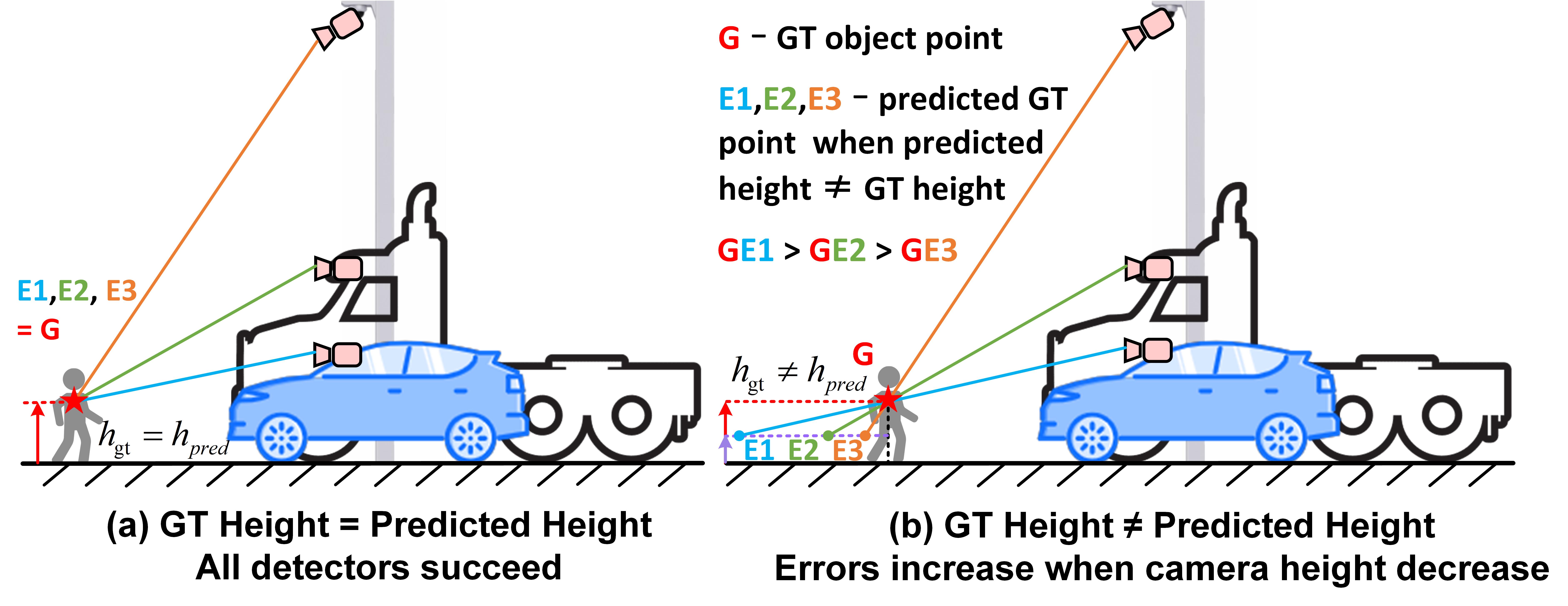
Figure 7: Distance error analysis caused by same height estimation error on different platform cameras.

Contributions. Theoretically, our proposed height-based pipeline entails: i) representation agnostic to distance, as visualized in Fig. 1, ii) friendly prediction owing to centralized distribution as displayed in Fig. 2, iii) robustness against extrinsic disturbance as illustrated in Fig. 3. Technically, we design a novel HeightNet and the projection module with less computational cost. Experimentally, experiments on various datasets and multiple depth-based detectors show the superiority of our method in both accuracy and latency.

5 Conclusion

We notice that in the domain of roadside perception, the depth difference between the foreground object and background quickly shrinks as the distance to the camera increases, this makes state-of-the-art methods that predict depth to facilitate vision-based 3D detection tasks sub-optimal. On the contrary, we discover that the per-pixel height does not change regardless of distance. To this end, we propose a simple yet effective framework, BEVHeight, to firstly predict the height and then project the 2D feature to 3D space to improve the detector. Through extensive experiments, BEVHeight surpasses BEVDepth baseline by a margin of 4.85% and 4.43% on DAIR-V2X-I and Rope3D benchmarks under the traditional clean settings, and by 26.88% on robust settings where external camera parameters changes. We hope our work can shed light on studying more effective feature representation on roadside perception.

Appendix A Appendix

A.1 Broader Impacts

Our work aims to develop a vision-based 3D object detection approach for roadside perception. The proposed method may produce inaccurate predictions, leading to incorrect decision-making for cooperative autonomous vehicles and potential traffic accidents. Furthermore, we propose a new perspective of leveraging height estimation to solve PV-BEV transformation, facilitating a high-performance and robust vision-centric BEV perception framework. Although considerable progress has been made with our proposed height net and height-based 2D-3D projection module, we believe it is worth further exploring how to combine height and depth estimations to extend to autonomous driving scenarios.

A.2 Dynamic Discretization

The height discretization can be performed with uniform discretization (UD) with a fixed bin size, spacing-increasing discretization (SID) [6] with increasing bin sizes in logspace, linear-increasing discretization (LID) [32]and our proposed dynamic-increasing discretization (DID) with adjustable bin sizes. The above four height discretization techniques are visualized in Fig. 8. Following DID strategy, the distribution of height bins can be dynamically adjusted with different hyper-parameter $\alpha$.

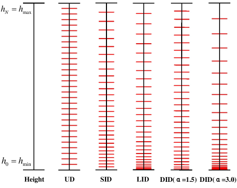
Figure 8: Height Discretization Methods. Height $h_{i}$ is discretized over a height range $[h_{min},h_{max}]$ into $N$ discrete bins. From left to right, these are uniform discretization (UD), spacing-increasing discretization (SID), linear-increasing discretization (LID) and the adjustable dynamic-increasing discretization(DID). For the dynamic-increasing discretization (DID) strategy, height bins with large $\alpha$ are more densely distributed when approaching the $h_{min}$ than the small hyper-parameter $\alpha$ conditions.

A.3 Results on V2X-Sim Dataset

To certify the effectiveness of our method in multi-view scenarios, we conduct experiments on V2X-Sim [17] simulation dataset that contains four surround roadside cameras. As shown in Tab. 9, our BEVHeight surpass the BEVDepth by more than 10.88%, 21.15% on vehicle and cyclist respectively, which verifies the effectiveness of our method.

Table 9: Comparison on the V2X-Sim Detection Benchmark.

Method	$\text{Vehicle}_{(IoU=0.5)}$			$\text{Cyclist}_{(IoU=0.25)}$
	Easy	Mod.	Hard	Easy	Mod.	Hard
BEVDepth [16]	81.99	81.39	81.31	45.95	45.93	45.90
BEVHeight	92.80	92.27	92.15	67.24	67.08	67.00

A.4 Effectiveness on multi depth-based Detectors

We extend our modules on BEVDepth[16] and BEVDet [10] on DAIR-V2X-I[39] and present the results here. Replacing the depth-based projection in BEVDepth[16], our method achieves a performance increase of 2.19%, 5.87%, 4.61% on vehicle, pedestrian and cyclist. Similarly, our approach surpasses the origin BEVDet by 8.56%, 5.35%, 8.60% respectively.

Table 10: Ablation studies on different depth-based methods. Here, we conduct the evaluation on DAIR-V2X-I val set, and report the results of three types of objects, vehicle (veh.), pedestrian (ped.) and cyclist (cyc.).

Method	VT	$\text{Veh.}_{(IoU=0.5)}$			$\text{Ped.}_{(IoU=0.25)}$			$\text{Cyc.}_{(IoU=0.25)}$
		Easy	Mod.	Hard	Easy	Mod.	Hard	Easy	Mod.	Hard
BEVDepth[16]	D	75.50	63.58	63.67	34.95	33.42	33.27	55.67	55.47	55.34
	H	77.78	65.77	65.85	41.22	39.29	39.46	60.23	60.08	60.54
BEVDet [10]	D	59.59	51.92	51.81	12.61	12.43	12.37	34.91	34.32	34.21
	H	69.42	60.48	59.68	18.11	17.81	17.74	44.69	42.92	42.34
VT denotes view transformation, D,H represents depth-based and height-based ones.

A.5 More Results on DAIR-V2X-I Dataset

Tab. 11 shows the experimental results of deploying our proposed approach on the DAIR-V2X-I[39] val set. Under the same configurations (e.g., backbone and BEV resolution), our model outperforms the BEVDepth[16] baselines by a large marge, which demonstrates the admirable performance of our approach.

Table 11: Comparison on the DAIR-V2X-I Detection Benchmark. Here, we report the results of three types of objects: Vehicle, Pedestrian and Cyclist. Each object is categorized into three settings according to the difficulty defined in  [39]. Our BEVHeight manages to surpass the BEVDepth baseeline over a margin of 2% - 6% under the same configurations.

Method	Scale of Detector		AP3D
			$\text{Vehicle}_{(IoU=0.5)}$			$\text{Pedestrian}_{(IoU=0.25)}$			$\text{Cyclist}_{(IoU=0.25)}$
	Backbone	BEV	Easy	Middle	Hard	Easy	Middle	Hard	Easy	Middle	Hard
BEVDepth[16]	R50	128x128	73.05	61.32	61.19	22.10	21.57	21.11	42.85	42.26	42.09
BEVDepth[16]	R101	128x128	74.81	62.44	62.31	24.49	23.33	23.17	44.93	44.02	43.84
BEVDepth[16]	R101	256x256	75.50	63.58	63.67	34.95	33.42	33.27	55.67	55.47	55.34
BEVHeight	R50	128x128	76.61	64.71	64.76	27.34	26.09	26.33	49.68	48.84	48.58
BEVHeight	R101	128x128	76.93	64.97	65.03	28.53	27.15	27.48	51.39	50.83	50.44
BEVHeight	R101	256x256	77.78	65.77	65.85	41.22	39.29	39.46	60.23	60.08	60.54

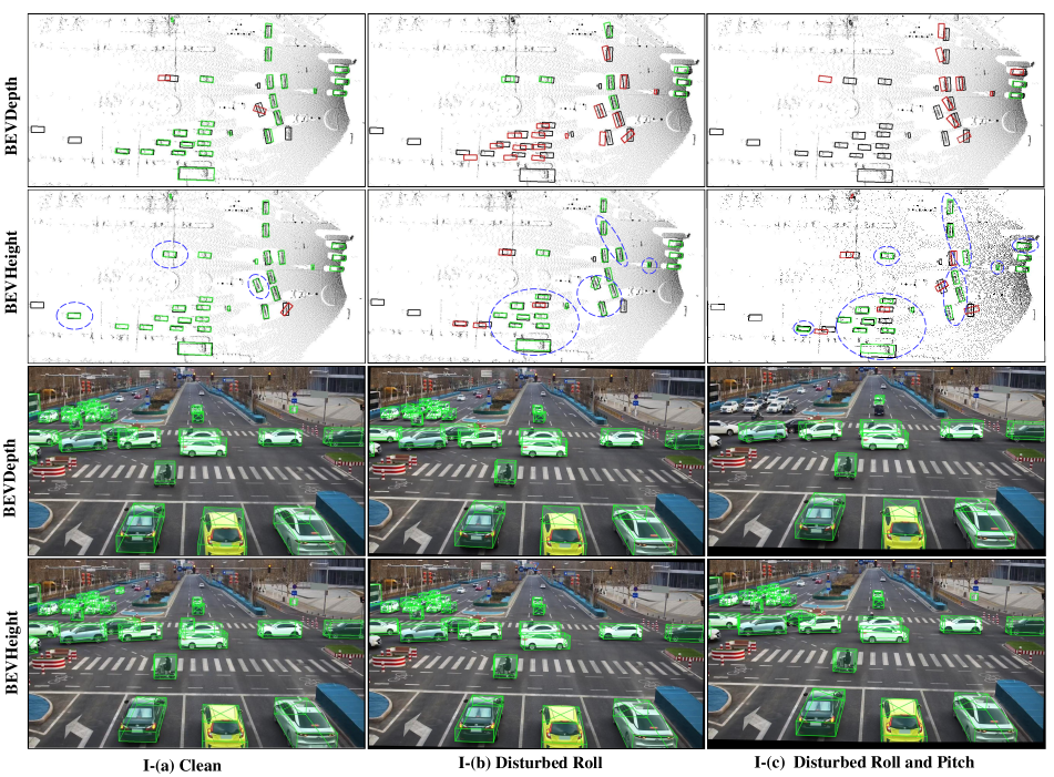
Figure 9: Visualization Results of BEVDepth and our proposed BEVHeight under the extrinsic disturbance. We use boxes in red to represent false positives, green boxes for truth positives, and black for the ground truth. The truth positives are defined as the predictions with IoU>0.5 for vehicle and IoU>0.25 for pedestrian and cyclist. I/II-(a) Clean means the original image without any processing; I/II-(b) Disturbed Roll denotes camera rotate 1 degree along roll direction; I/II-(c) Disturbed Roll and Pitch represents camera rotate 1 degree along roll and pitch directions simultaneously. We use blue dashed ovals to highlight the pronounced improvements in predictions.

Figure 10: Visualization Results of BEVDepth and our proposed BEVHeight under the extrinsic disturbance in another scene.

A.6 More Visualizations

In Fig. 9 and Fig. 10, we show more visualization results on the DAIR-V2X-I [39] dataset. As can be seen from the samples in I/II-(a) clean, our BEVHeight manage to detect objects in middle and long-distances. As for the extrinsic disturbance cases in I/II-(b) and I/II-(c), our method can still guarantee the detection accuracy in terms of cars, pedestrian and cyclist. It can be concluded that our method can significantly improve the accuracy in middle and long-distances and the robustness to extrinsic disturbance.

References

- [1] Garrick Brazil and Xiaoming Liu. M3d-rpn: Monocular 3d region proposal network for object detection. In Proceedings of the IEEE International Conference on Computer Vision, pages 9287–9296, 2019.
- [2] Garrick Brazil, Gerard Pons-Moll, Xiaoming Liu, and Bernt Schiele. Kinematic 3d object detection in monocular video. In European Conference on Computer Vision, pages 135–152. Springer, 2020.
- [3] Holger Caesar, Varun Bankiti, Alex H Lang, Sourabh Vora, Venice Erin Liong, Qiang Xu, Anush Krishnan, Yu Pan, Giancarlo Baldan, and Oscar Beijbom. nuscenes: A multimodal dataset for autonomous driving. In Proceedings of the IEEE/CVF conference on computer vision and pattern recognition, pages 11621–11631, 2020.
- [4] Shaoyu Chen, Xinggang Wang, Tianheng Cheng, Q. Zhang, Chang Huang, and Wenyu Liu. Polar parametrization for vision-based surround-view 3d detection. ArXiv, abs/2206.10965, 2022.
- [5] Jiaxun Cui, Hang Qiu, Dian Chen, Peter Stone, and Yuke Zhu. Coopernaut: End-to-end driving with cooperative perception for networked vehicles. In Proceedings of the IEEE/CVF Conference on Computer Vision and Pattern Recognition, pages 17252–17262, 2022.
- [6] Huan Fu, Mingming Gong, Chaohui Wang, Kayhan Batmanghelich, and Dacheng Tao. Deep ordinal regression network for monocular depth estimation. In Proceedings of the IEEE/CVF Conference on Computer Vision and Pattern Recognition, 2018.
- [7] Andreas Geiger, Philip Lenz, and Raquel Urtasun. Are we ready for autonomous driving? the kitti vision benchmark suite. In Proceedings of the IEEE/CVF Conference on Computer Vision and Pattern Recognition, pages 3354–3361, 2012.
- [8] Kaiming He, Xiangyu Zhang, Shaoqing Ren, and Jian Sun. Deep residual learning for image recognition. In Proceedings of the IEEE Conference on Computer Vision and Pattern Recognition, pages 770–778, 2016.
- [9] Junjie Huang and Guan Huang. Bevdet4d: Exploit temporal cues in multi-camera 3d object detection. arXiv preprint arXiv:2203.17054, 2022.
- [10] Junjie Huang, Guan Huang, Zheng Zhu, and Dalong Du. Bevdet: High-performance multi-camera 3d object detection in bird-eye-view. arXiv preprint arXiv:2112.11790, 2021.
- [11] Kuan-Chih Huang, Tsung-Han Wu, Hung-Ting Su, and Winston H Hsu. Monodtr: Monocular 3d object detection with depth-aware transformer. In Proceedings of the IEEE/CVF Conference on Computer Vision and Pattern Recognition, pages 4012–4021, 2022.
- [12] Lei Huang and Wenzhun Huang. Rd-yolo: An effective and efficient object detector for roadside perception system. Sensors, 22(21):8097, 2022.
- [13] Yanqin Jiang, Li Zhang, Zhenwei Miao, Xiatian Zhu, Jin Gao, Weiming Hu, and Yu-Gang Jiang. Polarformer: Multi-camera 3d object detection with polar transformers. arXiv preprint arXiv:2206.15398, 2022.
- [14] Alex H Lang, Sourabh Vora, Holger Caesar, Lubing Zhou, Jiong Yang, and Oscar Beijbom. Pointpillars: Fast encoders for object detection from point clouds. In Proceedings of the IEEE/CVF conference on computer vision and pattern recognition, pages 12697–12705, 2019.
- [15] Yinhao Li, Han Bao, Zheng Ge, Jinrong Yang, Jianjian Sun, and Zeming Li. Bevstereo: Enhancing depth estimation in multi-view 3d object detection with dynamic temporal stereo. arXiv preprint arXiv:2209.10248, 2022.
- [16] Yinhao Li, Zheng Ge, Guanyi Yu, Jinrong Yang, Zengran Wang, Yukang Shi, Jianjian Sun, and Zeming Li. Bevdepth: Acquisition of reliable depth for multi-view 3d object detection. arXiv preprint arXiv:2206.10092, 2022.
- [17] Yiming Li, Dekun Ma, Ziyan An, Zixun Wang, Yiqi Zhong, Siheng Chen, and Chen Feng. V2x-sim: Multi-agent collaborative perception dataset and benchmark for autonomous driving. IEEE Robotics and Automation Letters, 7(4):10914–10921, 2022.
- [18] Zhiqi Li, Wenhai Wang, Hongyang Li, Enze Xie, Chonghao Sima, Tong Lu, Qiao Yu, and Jifeng Dai. Bevformer: Learning bird’s-eye-view representation from multi-camera images via spatiotemporal transformers. arXiv preprint arXiv:2203.17270, 2022.
- [19] Yingfei Liu, Tiancai Wang, Xiangyu Zhang, and Jian Sun. Petr: Position embedding transformation for multi-view 3d object detection. arXiv preprint arXiv:2203.05625, 2022.
- [20] Yingfei Liu, Junjie Yan, Fan Jia, Shuailin Li, Qi Gao, Tiancai Wang, Xiangyu Zhang, and Jian Sun. Petrv2: A unified framework for 3d perception from multi-camera images. arXiv preprint arXiv:2206.01256, 2022.
- [21] Ilya Loshchilov and Frank Hutter. Decoupled weight decay regularization. arXiv preprint arXiv:1711.05101, 2017.
- [22] Xinzhu Ma, Yinmin Zhang, Dan Xu, Dongzhan Zhou, Shuai Yi, Haojie Li, and Wanli Ouyang. Delving into localization errors for monocular 3d object detection. In Proceedings of the IEEE/CVF Conference on Computer Vision and Pattern Recognition, pages 4721–4730, 2021.
- [23] Jinhyung Park, Chenfeng Xu, Shijia Yang, Kurt Keutzer, Kris Kitani, Masayoshi Tomizuka, and Wei Zhan. Time will tell: New outlooks and a baseline for temporal multi-view 3d object detection. arXiv preprint arXiv:2210.02443, 2022.
- [24] Jonah Philion and Sanja Fidler. Lift, splat, shoot: Encoding images from arbitrary camera rigs by implicitly unprojecting to 3d. In European Conference on Computer Vision, pages 194–210. Springer, 2020.
- [25] Cody Reading, Ali Harakeh, Julia Chae, and Steven L Waslander. Categorical depth distribution network for monocular 3d object detection. In Proceedings of the IEEE/CVF Conference on Computer Vision and Pattern Recognition, pages 8555–8564, 2021.
- [26] Danila Rukhovich, Anna Vorontsova, and Anton Konushin. Imvoxelnet: Image to voxels projection for monocular and multi-view general-purpose 3d object detection. In Proceedings of the IEEE/CVF Winter Conference on Applications of Computer Vision, pages 2397–2406, 2022.
- [27] Avishkar Saha, Oscar Alejandro Mendez Maldonado, Chris Russell, and R. Bowden. Translating images into maps. 2022 International Conference on Robotics and Automation (ICRA), pages 9200–9206, 2022.
- [28] Andrea Simonelli, Samuel Rota Bulo, Lorenzo Porzi, Manuel López-Antequera, and Peter Kontschieder. Disentangling monocular 3d object detection. In Proceedings of the IEEE/CVF International Conference on Computer Vision, pages 1991–1999, 2019.
- [29] Vishwanath A Sindagi, Yin Zhou, and Oncel Tuzel. Mvx-net: Multimodal voxelnet for 3d object detection. In 2019 International Conference on Robotics and Automation (ICRA), pages 7276–7282. IEEE, 2019.
- [30] Zhiying Song, Fuxi Wen, Hailiang Zhang, and Jun Li. An efficient and robust object-level cooperative perception framework for connected and automated driving. arXiv preprint arXiv:2210.06289, 2022.
- [31] Pei Sun, Henrik Kretzschmar, Xerxes Dotiwalla, Aurelien Chouard, Vijaysai Patnaik, Paul Tsui, James Guo, Yin Zhou, Yuning Chai, Benjamin Caine, et al. Scalability in perception for autonomous driving: Waymo open dataset. In Proceedings of the IEEE/CVF conference on computer vision and pattern recognition, pages 2446–2454, 2020.
- [32] Yunlei Tang, Sebastian Dorn, and Chiragkumar Savani. Center3d: Center-based monocular 3d object detection with joint depth understanding. arXiv: Computer Vision and Pattern Recognition, 2020.
- [33] Ching-Yu Tseng, Yi-Rong Chen, Hsin-Ying Lee, Tsung-Han Wu, Wen-Chin Chen, and Winston Hsu. Crossdtr: Cross-view and depth-guided transformers for 3d object detection. arXiv preprint arXiv:2209.13507, 2022.
- [34] Yue Wang, Vitor Campagnolo Guizilini, Tianyuan Zhang, Yilun Wang, Hang Zhao, and Justin Solomon. Detr3d: 3d object detection from multi-view images via 3d-to-2d queries. In Conference on Robot Learning, pages 180–191. PMLR, 2022.
- [35] Zengran Wang, Chen Min, Zheng Ge, Yinhao Li, Zeming Li, Hongyu Yang, and Di Huang. Sts: Surround-view temporal stereo for multi-view 3d detection. arXiv preprint arXiv:2208.10145, 2022.
- [36] Runsheng Xu, Hao Xiang, Zhengzhong Tu, Xin Xia, Ming-Hsuan Yang, and Jiaqi Ma. V2x-vit: Vehicle-to-everything cooperative perception with vision transformer. arXiv preprint arXiv:2203.10638, 2022.
- [37] Yan Yan, Yuxing Mao, and Bo Li. Second: Sparsely embedded convolutional detection. Sensors, 18(10):3337, 2018.
- [38] Xiaoqing Ye, Mao Shu, Hanyu Li, Yifeng Shi, Yingying Li, Guangjie Wang, Xiao Tan, and Errui Ding. Rope3d: The roadside perception dataset for autonomous driving and monocular 3d object detection task. In Proceedings of the IEEE/CVF Conference on Computer Vision and Pattern Recognition, pages 21341–21350, 2022.
- [39] Haibao Yu, Yizhen Luo, Mao Shu, Yiyi Huo, Zebang Yang, Yifeng Shi, Zhenglong Guo, Hanyu Li, Xing Hu, Jirui Yuan, et al. Dair-v2x: A large-scale dataset for vehicle-infrastructure cooperative 3d object detection. In Proceedings of the IEEE/CVF Conference on Computer Vision and Pattern Recognition, pages 21361–21370, 2022.
- [40] Kaicheng Yu, Tang Tao, Hongwei Xie, Zhiwei Lin, Zhongwei Wu, Zhongyu Xia, Tingting Liang, Haiyang Sun, Jiong Deng, Dayang Hao, et al. Benchmarking the robustness of lidar-camera fusion for 3d object detection. arXiv preprint arXiv:2205.14951, 2022.
- [41] Renrui Zhang, Han Qiu, Tai Wang, Xuanzhuo Xu, Ziyu Guo, Yu Qiao, Peng Gao, and Hongsheng Li. Monodetr: Depth-aware transformer for monocular 3d object detection. arXiv preprint arXiv:2203.13310, 2022.
- [42] Yunpeng Zhang, Jiwen Lu, and Jie Zhou. Objects are different: Flexible monocular 3d object detection. In Proceedings of the IEEE/CVF Conference on Computer Vision and Pattern Recognition, pages 3289–3298, 2021.
- [43] Benjin Zhu, Zhengkai Jiang, Xiangxin Zhou, Zeming Li, and Gang Yu. Class-balanced grouping and sampling for point cloud 3d object detection. arXiv preprint arXiv:1908.09492, 2019.
- [44] Xizhou Zhu, Han Hu, Stephen Lin, and Jifeng Dai. Deformable convnets v2: More deformable, better results. In Proceedings of the IEEE Conference on Computer Vision and Pattern Recognition, 2018.