Forecasting Intraday Power Output by a Set of PV Systems using Recurrent Neural Networks and Physical Covariates

Abstract

Accurate intraday forecasts of the power output by PhotoVoltaic (PV) systems are critical to improve the operation of energy distribution grids. We describe a neural autoregressive model which aims at performing such intraday forecasts. We build upon a physical, deterministic PV performance model, the output of which being used as covariates in the context of the neural model. In addition, our application data relates to a geographically distributed set of PV systems. We address all PV sites with a single neural model, which embeds the information about the PV site in specific covariates. We use a scale-free approach which does rely on explicit modelling of seasonal effects. Our proposal repurposes a model initially used in the retail sector, and discloses a novel truncated Gaussian output distribution. An ablation study and a comparison to alternative architectures from the literature shows that the components in the best performing proposed model variant work synergistically to reach a skill score of 15.72% with respect to the physical model, used as a baseline.

1 Introduction

Grids of PV systems have become an inevitable component in the modern and future energy distribution systems. However, due to weather conditions, the magnitude of PV power production is fluctuating, while the supply to consumers requires to be adapted to the demand at each point in time. Distribution system operators (DSOs) have increasing and specific requirements for PV power forecasts. Indeed, fluctuating renewables could cause operational issues (e.g. grid congestion), which call for active grid operation. In this context, fine-grained forecasts of PV power expected during the day to come are critical in view to facilitate operations. Also, many forecasting models issue point forecasts, but hardly characterize the uncertainty attached to their forecasts, when such information can be critical for a DSO in order to quantify and mitigate risks in the context of a trading strategy.

PV power production can be forecasted using a deterministic PV performance model [1]. It models the internals of a PV system, from the solar irradiance received to the electrical power produced using a set of physical equations (referred to by the shorthand term physical model in the remainder of this paper). Therefore, for each time step for which PV power has to be predicted, it needs a solar irradiance forecast, provided by a Numerical Weather Prediction (NWP) service, as inputs. The underlying hypothesis is that solar irradiance is fairly smooth over limited regional areas, and the production curve specific to a PV system will be mainly influenced by how it converts this solar energy to PV power according to its specifications. In [2], authors of the present paper introduced a model which performs intraday probabilistic forecasts of PV power production. It combines the physical model referred to above with a model based on Long-Short-Term Memory (LSTM) cells [3]. This kind of combination of a model based on a set of physical equations to a statistical model is sometimes coined as hybrid-physical in the solar energy literature [4]. For training and evaluation, it uses real data provided by Electris, a DSO in Luxembourg. Results show that this new model improves the baseline performance, while coping with local effects such as PV system shading. The former paper rather targets solar energy specialists, with little details unvealed about how the Machine Learning model acting as cornerstone to the approach has been designed and trained. The present paper aims at filling this gap, by providing entirely new material focusing on this complementary view. Specifically, the purpose of the present paper is to focus on neural time series forecasting aspects in the context of this application.

The specific contributions of the present work mainly focus on the design of a model architecture and a training procedure which meets the operational needs expressed by the DSO. The contributions of our applicative paper are:

• Repurposing an existing LSTM-based model [5], by casting the hybrid-physical approach in terms of statistical model covariates,

• Using PV system specifications as covariates in a univariate model,

• Designing a novel truncated Gaussian output component, which we plug in to the LSTM-based model.

In Section 2, we give a structured survey of the related work which positions the addressed applicative problem, and motivates which existing work could be reused or repurposed to suit our needs. After describing our model proposal in Section 3, we provide a thorough experimental evaluation in Section 4. Several variants of our model proposal are compared to alternative models from the literature, and an ablation study allows to emphasize the specific contribution of each of its components. Finally we recall some qualitative results to underline how local effects, tainting the PV performance model, are mitigated using our approach.

2 Related Work

In Section 2.1, we review seminal PV power forecasting methods. Then in Section 2.2, we survey time series forecasting as addressed in the literature on Machine Learning (ML), from the perspective of their repurposing potential to the PV power forecasting application. Finally, Section 2.3 focuses on the peculiarities in terms of forecasting structure and validation which come with ML approaches applied to time series forecasting.

2.1 PV Power Forecasting

Most approaches in PV power forecasting model the conversion chain of solar irradiance to electrical power in a PV system. Thus they follow a two-step approach: first, forecasting the solar irradiance, then converting this irradiance to PV power forecasts [6, 1]. The most common way to forecast solar irradiance relies on NWP systems such as the European Centre for Medium-Range Weather Forecasts (ECWMF) Ensemble Prediction System [7]. Everyday, it issues hourly regional forecasts for a range of meteorological variables (including solar irradiance) on the 10 days to come, thus including the intraday range. Intraday may be defined as up to 6h forecast horizons in the literature [4]. In this paper, for experimental simplicity, we deviate from this definition by considering intraday as the next 24h, starting at midnight of the same day. The PV power data described in Section 4.1 is collected each day at 6:00 CET by Electris, and twilight time is generally before 22:00 CET in Luxembourg. As we exclude night time slots from the metrics presented in Section 4.2, our intraday definition is roughly equivalent to that used in the context of the Nord Pool power exchange market. In view to improve NWP system outputs, or to avoid having to rely on such systems, solar irradiance can also be forecasted using statistical methods and ML models. The simplest include persistence models, which are often adjusted using clear sky models [8]. [9] also review various ML techniques which have been employed to this purpose, e.g., AutoRegressive (AR) models, Feed-Forward Networks (FFN) and k-Nearest Neighbors. In this range of contributions, [10] address the intraday hourly prediction of solar irradiance using an ensemble of FFN models. Specifically, they implement rolling forecasts by specializing each model to a current time and a prediction horizon.

PV power forecasting is reviewed in detail by [4]. In this domain, several approaches aim at modelling directly the series of PV power values, without having to rely on solar irradiance forecasts. [11] propose short-term forecasts ($<$30mn) which exploit cross-correlation of PV measurements in a grid of PV systems. They hypothesize that clouds casting over a given PV system have lagged influence on other systems downwind. They optimize associated time lag and cloud motion vector. [12] also consider a spatially distributed set of PV panels. They directly use PV power values, without converting proxy information such as solar irradiance or cloud density. Similarly to [11], they focus on correlations among stations to help accounting for intermittency due to clouds.

[13] present AR approaches to PV power forecasting. They focus on forecasting one and two hours ahead, where NWP models tend to under-perform. Several models are compared, among which are persistence, linear models such as AutoRegressive Integrated Moving Average (ARIMA) [14], and FFN. They found out that FFN perform the best, with improvements brought by the optimization of FFN parameters, input selection and structure using a Genetic Algorithm.

2.2 ML approaches for time series forecasting

Among other related work, Section 2.1 surveyed some contributions which involved ML methods in view to forecast solar irradiance and PV power production. In this section, we generalize this view, by surveying recent work in time series forecasting at large. Methods in this section were generally not applied to the applicative context considered in the present paper, but could be repurposed a priori. Besides neural and ARIMA models, seminal ways to forecast time series include the Croston method, which is an exponential smoothing model dedicated to intermittent demand forecasting [15]. It is notably used as baseline method in [5], along with the Innovation State-Space Model (ISSM) [16].

Modern, so-called deep neural network architectures, such as the Long-Short-Term Memory (LSTM) [3] and the Gated Recurrent Unit (GRU) [17], exploit the sequential structure of data. Even though recurrent models such as the LSTM would appear as outdated, they are still popular in the recent literature thanks to improvements to training and inference procedures carried by modern toolboxes such as Tensorflow [18] or MXNet [19], as well as the encoder-decoder mechanism, in which a context sequence is encoded and conditions the prediction of the target sequence. It has been initially codified for the GRU, and transferred to the LSTM, leading to continued usage in recent contributions [20, 5]. These models contrast with the seminal Feed-Forward Network (FFN), in which all layers are fully connected to previous and next layers, up to the activation layer [21].

Salinas et al. propose DeepAR, which implements flexible forecasting for univariate time series [5]. Formally, it defines a context interval (a chunk of past values) and a forecasting interval (the set of values to be forecasted), and the model is optimized end-to-end w.r.t. the whole forecasting range. This contrasts with linear models such as ARIMA, which are optimized for one time step ahead forecasts. Also, instead of point forecasts, DeepAR predicts model parameters, which can be used to compute sample paths and empirical quantiles, then potentially used by the DSO to adjust its trading strategy in the context of this paper. In this case, a family of probability distributions has to be chosen so as to fit the time series at hand. The model was initially aimed at retail business applications, but it can be adapted to other types of data just by changing the family of the output probability distribution. It is based on the LSTM model architecture. The model supports the adjunction of covariates, i.e., time series which are available for both context and forecasting intervals at inference time. By repeating the same value for the whole intervals, static covariates are also supported.

In retail applications, input data may have highly variable magnitude (e.g., depending on item popularity or time in the year). The authors observe an approximate power law between item magnitude and frequency (i.e., values are less likely as they get large, and reciprocally). They claim that grouping items to learn group-specific models or performing group-specific normalizations, as previously done in the solar and PV power forecasting literature [13, 10] are not good strategies in such case. They propose a simple alternative scheme, where samples are scaled by a factor computed using the context interval.

A convolutional encoder is tested by Wen et al. in the context of their multi-horizon quantile forecaster [22]. Instead of forecasting probabilistic model parameters, this model directly forecasts quantiles in a non-parametric fashion. However, it suffers from the quantile crossing problem: forecasted values may have ranks inconsistent with the quantile they are attached too. [23] is another alternative to DeepAR. Similarly to [22], it does not rely on probability distribution outputs, and implements conditional quantile functions using regression splines instead. Spline parameters are fit using a neural network directly minimizing the Continuous Ranked Probability Score (CRPS) [24], which is then used as a loss function. This results in a more flexible output distribution, and an alternative to other flexible schemes (e.g. mixture of distributions in the context of [5]). However, it currently lacks a publicly available implementation.

Multivariate forecasting consists in modelling and forecasting multiple time series simultaneously, by contrast to univariate forecasting. The seminal way to achieve this, is with the Vector AutoRegression (VAR) model, which is an extension of the linear autoregressive model to multiple variables [25]. As this model has hard time dealing with many variables (e.g., items in the retail domain), neural network-based models such as DeepVAR were designed as an alternative [26]. It can be thought of as a multivariate extension to [5]. DeepVAR models interaction between time series, e.g., as resulting from causality or combined effects. It uses a Copula model, which models interactions between time series, and elegantly copes with time series of varying magnitude, alleviating the need for an explicit scaling mechanism. A single multivariate state variable underlying a LSTM model is used for all time series. They also define a low-rank parametrization, which opens the possibility to deal with a very large number of time series.

Some prior work involved deep learning in the context of PV power forecasting. For example, [27] consider one hour ahead forecasts (instead of intraday as aimed at in this paper). They used a single LSTM layer without the encoder-decoder mechanism, limited to point forecasts. Data for two PV sites is used for the experiments, with roughly the same power magnitude for both sites (approx. 3.5kW). Models are trained for each site separately. Alternatively, in this paper we address all sites with a single model in a scale free approach, dealing with an arbitrary number of sites with little to no model size overhead. Finally, the locations associated to the datasets are subject to a dry climate, which is simpler to predict [13]. Our application testbed is a temperate area, subject to frequent and abrupt changes on a daily basis, therefore much more challenging to predict. [28] also address PV power forecasting, by decorrelating scale free forecasts using LSTM, from seasonal effects modelled separately using time correlation features and partial daily pattern prediction. However, they focus on forecasts aggregated at a daily scale, when we consider hourly data in this paper. In addition, our approach is end-to-end, with seasonal effects modelled as time covariates, as allowed by the DeepAR model [5].

[29] present a regional PV power forecasting system, with hourly resolution up to 72h ahead. Their approach combines clustering and numerical optimization, and it is compared to regression methods such as ElasticNet [30], SARIMAX [31], or Random Forests [31]. Their approach is not autoregressive, rather they directly predict future PV power from solar irradiance and temperature forecasts obtained from a proprietary system which refines NWP forecasts according to local conditions. Alternatively, our approach tries to combine the benefits of using physical model forecasts (fed periodically by a NWP system) as covariates in an autoregressive model of the PV power time series. We observe that this effectively implements the hybrid-physical approach, which combines the output of a physical model to a machine learning model [4]. In an early work, Cao and Lin [32] used NWP covariates in the context of a neural network to perform next hour and aggregated daily solar irradiance forecasting. More recently, several models allow to combine continuous covariates to each time slot in a forecasting interval [22, 5, 33, 34]. The model which we describe in Section 3, and the experiments in Section 4, involve models from this family.

2.3 Forecast structure and validation

Figure 1 distinguishes regular forecasts from rolling forecasts, which are the two main strategies to consider for extracting fixed sized blocks from time series [35]. For simplicity, the figure considers hourly forecasts and 24-hour context and forecasting intervals, but the definition is straightforward to generalize. In brief, two consecutive regular forecasts are offset by the size of the forecasting interval, when rolling forecasts are offset by the frequency of the time series (hourly, in Figure 1). In other words, with 24-hour forecasting and context intervals, regular forecasts happen on the same time every day, whereas rolling forecasts are issued every hour for the whole forecasting interval. In this process, forecasts beyond the next hour are refreshed every hour.

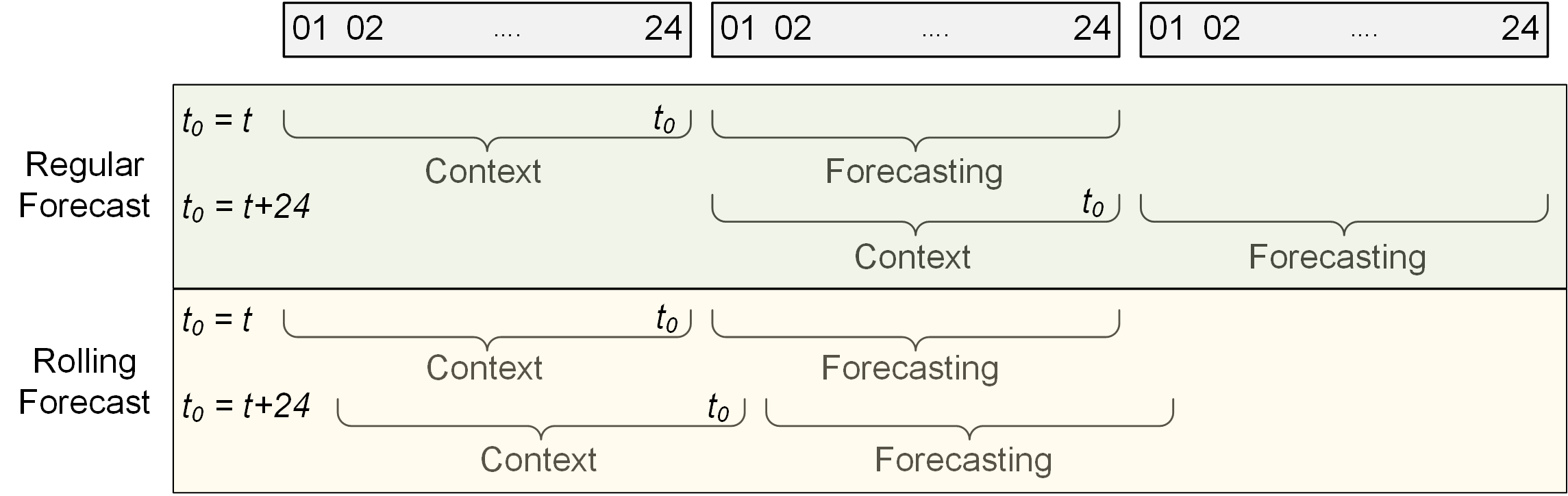
Figure 1: Distinction between regular and rolling forecasts. $t_{0}$ denotes the present time step in the context of a given data sample.

Works such as [29] consider regular forecasts, as the forecast time is tied to availability of NWP data. As the physical covariates we use in our our work are also tied to forecasts issued from a NWP service, and the data we use in our experiments in Section 4 is only collected daily by the DSO, regular forecasts are a requirement in our work too. Alternatively, [10] address rolling forecasts by having a distinct model for each possible starting time in the day. Let us note that some models (e.g., [5]) allow to encode seasonal information on the predicted time steps (e.g. hour in day, day in week) as covariates (referred to as time covariates later on). Therefore, they can be used indistinctively with regular and rolling forecasts, provided an adapted training set is available. Also, contrasting to [28], this means that modelling periodicity and seasonality explicitly is not needed, as the model then directly combines this additional input to time series data.

[36] discuss the problem of cross-validation, and more generally validation, in the context of time series forecasting. Original formulations of cross-validation methods often assume that data items are independent. They cannot be used out of the box with time series, as the sequential structure of the latter invalidates the underlying hypotheses. They recognize that the seminal way to validate models with time series is to train a model using the first $t_{0}$ values, and validate using the last $T-t_{0}$ values. However, this way is hardly compatible with cross-validation schemes, and yields weak test error estimations. In virtue of the bias-variance tradeoff [37], this issue has moderate impact on models with strong bias such as linear models. However, over-parametrized models, such as most neural models presented in Section 2.2 (e.g. [5, 26, 23, 22]) can be significantly affected, and exhibit a strong tendency to overfit. For mitigation, [36] recommend blocked cross-validation, in which time series segments of size $\tau<<T$ are used for independent training and validation for model selection and test error computation. As we also use deep learning as a building block in our approach, we carefully consider these recommendations in our experimental design (see Section 4).

3 Model Description

The survey of related works in Section 2 led us to choose DeepAR [5] as a framework to develop our implementation. We adapted the official implementation of the model [38] to suit our needs. Another model which offers the relevant flexibility as well as a public implementation is the model by Wen et al. [22]. We will compare to this model in our experimental section.

Alternatively, PV sites could have been considered as dimensions in a multivariate forecasting problem, thus possibly forecasting all sites at a given time at once using DeepVAR [26]. However, its limitation to static covariates prevents us from implementing the projected approach, which uses forecasts from the physical model as covariates as means to build upon them. Also, it is unclear how new PV sites, as well as missing values, which are pretty common as PV sites may witness independent breakdowns and interruptions of measurements or data communication (see Section 4.3 for a quantitative account), can be handled with such multivariate modelling. Alternatively, we choose to model the PV site using covariates in the context of a univariate model. We will test the value of these covariates in our ablation study in Section 4.

3.1 DeepAR model

In the remainder of the paper, for clarity of the derivations, scalar variables are represented in normal font, vector variables in bold font, and matrix variables in capital bold font. This section 3.1 essentially paraphrases [5], but ensures the present paper is self-contained, while introducing the necessary formalism in general terms.

Let us assume we have a data set of $N$ univariate time series, each with fixed size $T$. Each observed time series in $\{\mathbb{z}_{n}\}_{n\in 1,\dots,N}$ may relate to an item in store in the retail context, or to a distinct PV system in the context addressed in this paper. $t_{0}\in[1,\dots,T]$ denotes the present time, i.e. the latest time point for which we assume $z_{n,t}$ is known when issuing the forecast. $[1,\dots,t_{0}]$ is then the context interval, and $[t_{0}+1,\dots,T]$ is the forecasting interval. Let us note that each $t\in[1,\dots,T]$ is merely associated to the position of values within each sample $\mathbb{z}_{n}$; this is not inconsistent with the fact that $t$, in the context of two different samples $n$ and $n^{\prime}$, may be tied with different absolute points in time, e.g. referring to two different days if chunking the data as described in Section 4.3. The goal of the model is then to forecast $\mathbb{z}_{n,t_{0}+1:T}=[z_{n,t_{0}+1},\dots,z_{n,T}]$ with the knowledge of $\mathbb{z}_{n,0:t_{0}}=[z_{n,0},\dots,z_{n,t_{0}}]$. We also consider a set of covariates $\mathbb{X}_{n,1:T}=[\mathbb{x}_{n,1},\dots,\mathbb{x}_{n,T}]$ which are known for $t\in[1,\dots,T]$, even at time $t_{0}$.

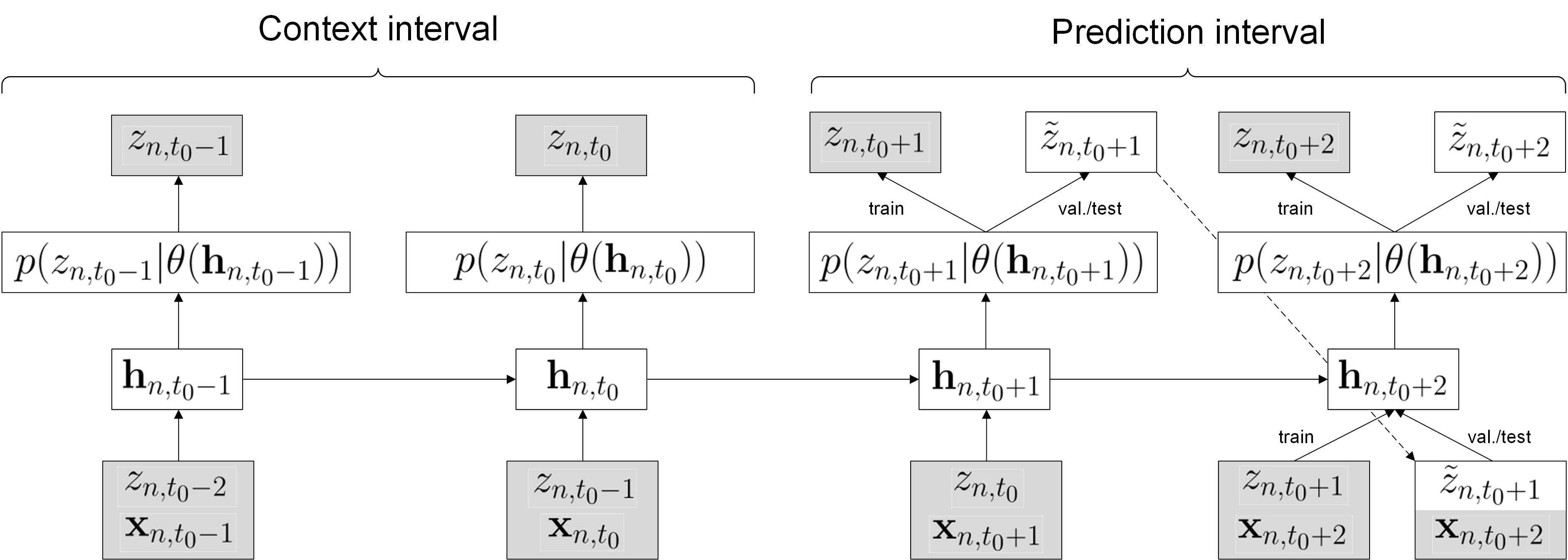
Figure 2: Illustration of the DeepAR model. Observed variables are represented as shaded boxes, and latent variables as blank boxes. For the context interval, $z$ variables are always known. For the forecasting interval, the model behaves differently at training and test time. At test time, $\tilde{z}$ variables are sampled according to $p$, forming sample paths. Plain lines represent dependencies between random variables, and the dashed line highlights the reinjected sample.

In this context, the model is defined by the following product of likelihood factors, also summarized in Figure 2:

$$Q_{\Theta} =\prod_{n=1}^{N}\prod_{t=t_{0}+1}^{T}{q_{\Theta}(z_{n,t}|\mathbb{z}_{n,1:t-1},\mathbb{X}_{n,1:T})}$$

$$=\prod_{n=1}^{N}\prod_{t=t_{0}+1}^{T}{p(z_{n,t}|\theta(\mathbb{h}_{n,t},\Theta))}$$ (1)

The model is both autoregressive and recurrent, as state variable:

$$\mathbb{h}_{n,t}=\Theta(\mathbb{h}_{n,t-1},z_{n,t-1},\mathbb{x}_{n,t})$$ (2)

is obtained from LSTM model $\Theta$ in which the state variable and observation of the previous time step are both reinjected. The model also depends on parametrized function $\theta$, which learns the mapping between the state variable $\mathbb{h}$ and parameters of the probability distribution $p$.

In effect, as seen in Figure 2, at training time, $\mathbb{z}_{n}$ is known for all $t\in[1\dots T]$, even the forecasting interval. The $z_{n,t}$ boxes on top of the diagram serve to compute losses then backpropagated to the model. However at test time actual observations are not available for the forecasting interval, so we sample $\tilde{z}_{n,t}\sim p$, and inject them as proxy observations. Doing so yields sample paths, which can be repeated and serve to compute empirical quantiles in the forecasting interval, instead of simple point estimates. In this paper, when point estimates $\hat{z}_{n,t}$ are needed, we take them as the empirical median of a set of sample paths. In Figure 2, we can see that the LSTM encodes the context interval into $\mathbb{h}$, which is then decoded for the forecasting interval. The same LSTM model $\Theta$ is used for encoding and decoding.

The negative log of expression (1) is used as the loss function for training all parameters in the model in an end-to-end fashion. The form of function $\theta$ depends on the probabilistic model in expression (1): for example, if $p$ is chosen as a Gaussian, appropriate functions would be:

$$\theta_{\mu}(\mathbb{h}_{n,t}) =\mathbb{w}_{\mu}\mathbb{h}_{n,t}+b_{\mu}$$

$$\theta_{\sigma}(\mathbb{h}_{n,t}) =\log(1+\exp(\mathbb{w}_{\sigma}\mathbb{h}_{n,t}+b_{\sigma}))$$ (3)

We note that the softplus function in (3) ensures $\sigma$ is mapped as a positive real number. Among possible probabilistic models and mapping functions, the official DeepAR implementation [38], used in the experiments for this paper, features Gaussian, Student, negative binomial, and mixture distributions. The mixture distribution composes several distributions from the same nature using mixture weights, which have their dedicated $\theta$ function.

3.2 Positive Gaussian likelihood model

As PV power measurements are bound to be non-negative real numbers, a contribution of this paper is to allow for the Gaussian distribution to be truncated from below at 0 (the upper limit remaining $+\infty$), referred to as the positive Gaussian distribution in the remainder of this paper. Formally this yields:

$$p(z_{n,t}|\theta_{\mu},\theta_{\sigma})=\frac{1}{\sigma\sqrt{2\pi}}\frac{\exp{(-\frac{1}{2}\frac{(z_{n,t}-\theta_{\mu})^{2}}{{\theta_{\sigma}}^{2}})}}{1-\Phi(-\frac{\theta_{\mu}}{\theta_{\sigma}})}$$ (4)

With $\Phi$ the cumulative distribution function of the standard Gaussian (i.e., with mean 0 and standard deviation 1). Besides adapting the loss function (see Equation (1)) to this new probability distribution function, the same $\theta_{\sigma}$ function as the Gaussian distribution can be used. To make sure the range of $\theta_{\mu}$ is also positive, for the positive Gaussian we use:

$$\theta_{\mu}(\mathbb{h}_{n,t})=\log(1+\exp(\mathbb{w}_{\mu}\mathbb{h}_{n,t}+b_{\mu}))$$

From an application of the Smirnov transformation [39] to the case at hand, samples from a positive Gaussian distribution can be obtained as:

$$\tilde{z}=\Phi^{-1}\Biggl{(}\Phi\bigl{(}-\frac{\theta_{\mu}}{\theta_{\sigma}}\bigr{)}+\tilde{u}\biggl{(}1-\Phi\bigl{(}-\frac{\theta_{\mu}}{\theta_{\sigma}}\bigr{)}\biggr{)}\Biggr{)}\theta_{\sigma}+\theta_{\mu}$$ (5)

where $\tilde{u}$ is a uniform sample in $[0,1]$.

4 Experiments

4.1 Data

Section 3 presented the forecasting model underlying our experiments in general terms, but here we recall that we focus on a specific application and its peculiarities: forecasting the power output of a set of PV systems.

The variable to forecast ($z$ in Section 3) is the average power output of a PV system during the hour to come in Watts. As hypothesized in Section 2.3, it is thus a hourly time series. For our experiments, we used data recorded by 119 PV systems located in Luxembourg between 01/01/2020 and 31/12/2021. They are dispatched in a relatively small (4 $\times$ 4 km) area. These PV systems are managed by Electris, a DSO in Luxembourg which collaborated with the authors of this paper in the context of a funded research project. Besides PV power measurements, each time step is associated to intraday, day-ahead, and 2 days ahead forecasts by the physical model described in [1]. We add these tier forecasts to the set of covariates used by the model ($\mathbb{X}$ in Section 3) along with time covariates mentioned in Section 2.3, as they will be available beforehand for the forecasting interval.

The model also supports the adjunction of static covariates, which are constant for a given sample. Relating to Section 3, we note that this simply amounts to set associated $\mathbb{x}_{n,1:T}$ to a constant. In the context of the present work, we consider a system ID categorical feature, which is simply the system ID converted to a categorical feature with 119 modalities. We also consider system description continuous features. Among the set of descriptors provided by system vendors and characteristics of their setup, we retain the following features as they are expected to influence PV power curves and magnitude: the exposition of the system (in degrees), its inclination (in degrees), its nominal power (in Watts) and its calibration factor (unitless, tied to the system on-site setup). As the DeepAR implementation expects normally distributed features, we standardize features so that they have zero mean and unit standard deviation.

As the nomimal power of our PV systems varies over a large range (from 1.4kW to 247kW), a scaling scheme is necessary to properly handle measured values. As mentioned in Section 2, we address this as implemented in DeepAR by dividing all measurements in a given sample by $\frac{1}{t_{0}}\sum_{1}^{t_{0}}{|z_{t}|}$. Also, as physical model outputs are expected to be distributed similarly to their associated measurements, they are normalized likewise.

4.2 Loss function and metrics

The sum of negative log-likelihoods of observations $z_{n,t}$ (on top of Figure 2) is used as a loss function to fit all model parameters $\{\mathbb{w}_{\mu},\mathbb{w}_{\sigma},\Theta\}$ in an end-to-end fashion. As commonly done in the literature (see Section 2.2), we use a fixed size for the context and forecasting intervals in our experiments. As we are interested in intraday regular forecasts (see Section 2.3), with hourly data this means that the forecasting interval has size 24. Being tied to the ECMWF NWP service, the physical model forecasts for the 3 days to come are computed each day early in the morning, but before the sunrise, so while PV power is still obviously zero. For simplicity, we thus choose midnight as the reference time in day for the regular forecasts (i.e., $t_{0}$ in Section 3). In this context, 24h, 48h and 72h physical covariates associated to predicted time step $t_{0}+h$ will have been issued at time steps $t_{0}$, $t_{0}-24$ and $t_{0}-48$, respectively.

As the maximal horizon of the collected NWP forecasts is 72h, and we previously set the intraday forecasting interval as 24h, as a rule of thumb we used 48h as the context interval so that a training sample covers 72h. In practice, preliminary tests showed that using a larger context interval would not bring visible improvements, and using a multiple of the forecasting interval size facilitates the creation of train and test data sets.

To measure model performance, we consider metrics based on RMSE (Root-Mean-Square Error) and MAE (Mean Absolute Error). The former are common in energy utility companies, notably as they penalize large errors [40], and the latter is consistent with our model, as forecasts are obtained by taking the median of sample paths [41]. We define normalized versions of these metrics as:

$$\text{nRMSE}(\hat{\mathbb{Z}},\mathbb{Z}) =\sqrt{\sum_{n=1}^{N}{\frac{1}{N}\frac{\frac{1}{T-t_{0}}\sum_{t_{0}+1}^{T}(\hat{z}_{nt}-z_{nt})^{2}}{P_{n}^{2}}}}$$ (6)

$$\text{nMAE}(\hat{\mathbb{Z}},\mathbb{Z}) =\sum_{n=1}^{N}{\frac{1}{N}\frac{\frac{1}{T-t_{0}}\sum_{t_{0}+1}^{T}|\hat{z}_{nt}-z_{nt}|}{P_{n}}}$$ (7)

with $P_{n}$ the nominal power of PV system $n$, $\hat{\mathbb{Z}}=\{\hat{z}_{nt}\}$ the estimated point forecast, and $\mathbb{Z}=\{z_{nt}\}$ the observed power. The normalization in Equations (6) and (7) allows to measure the performance of a point estimate forecast in such way that PV systems with larger nominal power do not dominate the error metric. This is a field requirement, as PV systems have private owners, who have to be treated equally, irrespective of the nominal power of their system. In practice, nMAE can be interpreted as a percentage of the PV system nominal power. For the sake of consistency with our model, we focus primarily on this metric, while also reporting nRMSE in Section 4.6. To evaluate the performance of a proposed system w.r.t. a reference, the skill score is derived from nMAE as:

$$\text{Skill score}=1-\frac{\text{nMAE}(\hat{\mathbb{Z}},\mathbb{Z})}{\text{nMAE}(\hat{\mathbb{Z}}_{\text{ref}},\mathbb{Z})}$$ (8)

As presented in Section 3, the models trained in the context of this work output prediction quantiles. We use the median as the point estimate forecast; in addition, we compute the CRPS metric [24], commonly used in related work [23, 5, 29], which rates the quality of prediction quantiles as a whole:

$$\text{CRPS}(F^{-1},\mathbb{Z}) =\frac{1}{N(T-t_{0})}\sum_{n=1}^{N}\sum_{t=t_{0}+1}^{T}\int_{0}^{1}{2\Lambda_{\alpha}(F^{-1}(\alpha),z_{nt})d\alpha}$$ (9)

$$\Lambda_{\alpha}(F^{-1}(\alpha),z_{nt}) =(\alpha-\mathcal{I}_{[z_{nt}<F^{-1}(\alpha)]})(z_{nt}-F^{-1}(\alpha))$$

with $F^{-1}$ the quantile function of the predictor (which returns the quantile level in Watts associated to a probability $\alpha\in]0,1[$), $\Lambda_{\alpha}$ the quantile loss, and $\mathcal{I}_{[\text{c}]}$ the indicator function associated to logical clause $c$. As discussed in Section 3, the quantile function is estimated empirically using a set of sample paths $\{\hat{\mathbb{z}}_{n}\}$. CRPS of course penalizes when observations are far from the median output by the model, but the penalty is increased if this difference is large while the model is excessively confident, as reflected, for example, by a narrow 90% prediction interval (i.e., the interval between the 5% and the 95% quantiles). In other words, this allows to penalize models which are excessively confident, and somehow reward models which are able to better estimate the expected accuracy of their point forecast. In our experiments, we use 100 paths per sample, which can be used as input to return empirical quantiles.

PV power is naturally zero at night time. Therefore, including these time steps in metric computation is likely to bias nMAE and CRPS towards 0. To prevent this, we exclude time steps associated to a solar zenith angle greater than $85^{o}$ [42] in Equation (6), (7) and (9).

4.3 Validation scheme

Following recommendations by [36], we create training samples by cutting the data set in fixed size 72h segments, with $t_{0}$ in each segment being midnight 24h before the end of the segment. Assuming we extracted the segment at the beginning of the available data, we then shift the offset 24h forward, so that the next segment includes the previous forecasting interval in its context interval (see, e.g., top of Figure 1). As we treat all PV systems as independent time series, this results in $O(CD)$ series, with $C$ the number of PV systems and $D$ the number of values $t_{0}$ can take in the original time series according to the segmentation method defined above.

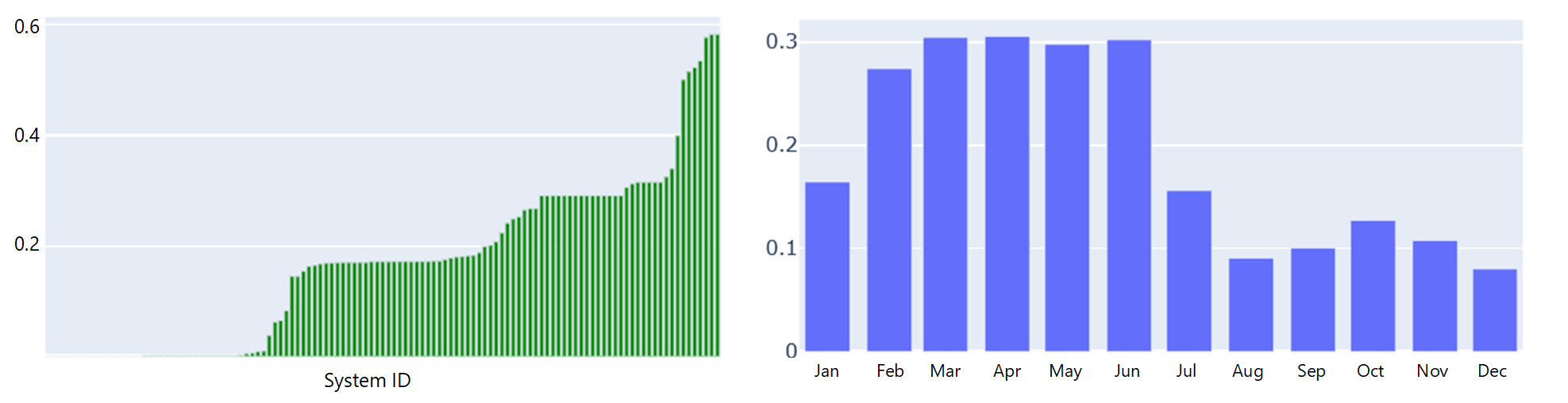
Figure 3: l.h.s.: Proportion of missing values per system. r.h.s.: Proportion of missing data per associated month.

Our number of PV systems and temporal collection bounds would yield 86989 samples. However, PV systems may exhibit missing or erroneous measurements due to several reasons (e.g., power outage, bad manipulation, faulty sensor). Figure 3 summarizes how missing values are distributed in the data set. The l.h.s. of Figure 3 shows that missing values are not uniformly distributed across PV systems. Approximately one third has no missing value, another third has a bit less than 20% of missing values, and the last third between 25% and 50%. The under-representation of this last third can be problematic. The r.h.s. of Figure 3 shows that these missing values are not evenly distributed in time: this indicates that a group of systems may have been offline for a contiguous time frame during late winter and spring. Actually, most missing values are linked to systems started later than the others in year 2020. The associated periods are therefore under-represented, but we note that any month has at most 30% missing data. In the remainder, we consider that this bias remains in a range which makes uniform sampling w.r.t. time acceptable for building training batches. In order to facilitate processing, and as samples cuts are aligned with day frames, we detect and exclude days matching one of the following patterns: more than two consecutive missing values, measurements blocked to a constant value, visual inspection for aberrant values. This results in 67666 valid day frames.

The PV systems are distributed in a relatively small area in Luxembourg: therefore, it is expected that forecasting intervals for different systems but same absolute time attached to $t_{0}$ will be highly correlated. In order to validate this intuition, we computed all $D$ intraday correlation matrices between systems in our data set. Specifically, we defined intraday time steps (excluding nightly time steps) as observations and PV systems as variables, resulting in $D\frac{C(C-1)}{2}$ distinct correlation values. We observe that the median of the distribution of these correlation values is 0.95, which confirms a very high correlation between systems for a given day. As a consequence, sampling uniformly training, validation and test sets in the $O(CD)$ series would result in data leakage, i.e., the model will be able to overfit without harming test error as identical samples (up to scale) will be scattered in training, validation and test sets. Let us note an unexpected positive benefit of this strong intraday correlation: the under-representation of some systems is then much less problematic. The only remaining issue would pertain to estimating the parameters associated to the static categorical modalities of these systems, if using system ID static covariates. We hypothesise that at least 50% of represented day frames is sufficient to perform this estimation.

To prevent the data leakage problem, we first group the samples by the absolute time attached to their respective $t_{0}$, and sample 60% of the $D$ time steps as the training set. We use a static temporal pattern, in order to ensure that each month and season is represented fairly evenly. Validation and test sets are uniformly sampled as half of the remaining 40% irrespective of the PV system, which is not an issue as the goal of validation error is to be an estimate of the test error, provided parameters are not explicitly fitted on the former. The validation set is used to implement early stopping, and select the model before it starts to overfit. The test set serves to compute the metrics described in Section 4.2. To choose the cut between validation and test, and ensure validation error is a fair proxy of the test error, we resample cuts until the validation and test nMAE between ground truth and intraday physical model forecasts (which are considered as constant and known in advance, and are the most relevant baseline to compare to) are equal up to a small threshold. Using the cutting procedure defined so far, we obtain 40670 training, 13498 validation and 13498 test samples.

4.4 Hyper-parameters

The models were trained using the Adam optimizer with learning rate $10^{-3}$, batch size 64, for 200 epochs. Samples are reshuffled at the beginning of each epoch. In the end, we implement a form of early stopping, by selecting the model with best validation nMAE. DeepAR uses 2 LSTM layers by default, we stick to this parametrization. Two free parameters remain then: the LSTM hidden layer size, and the number of components when a mixture distribution output is used. Figure 4 shows the results of a hyper-parameter search of these parameters using the positive Gaussian distribution as mixture components, as it is the distribution used in the model yielding the best results in Table 1. Median results from 6 independently trained models are displayed in the graphs, along with $\pm 1$ standard deviation error bars. We first use 100 as an initial guess of the hidden layer size, and vary the number of components used by model 1 (see Table 1, and Figure 4a). Except with only one component, the performance is good for all number of components, and best for 5 components. Then, using 5 components, we test hidden layer sizes between 20 and 500. Results are significantly better with size 40 (Figure 4b). Finally, we try to refine the number of components using hidden layer size 40, and excluding models with only one component as this setting was visibly irrelevant. Using 5 or 6 components stands out (Figure 4c); to give a bonus to parsimony, we retain 5 components for the remainder of the experiments.

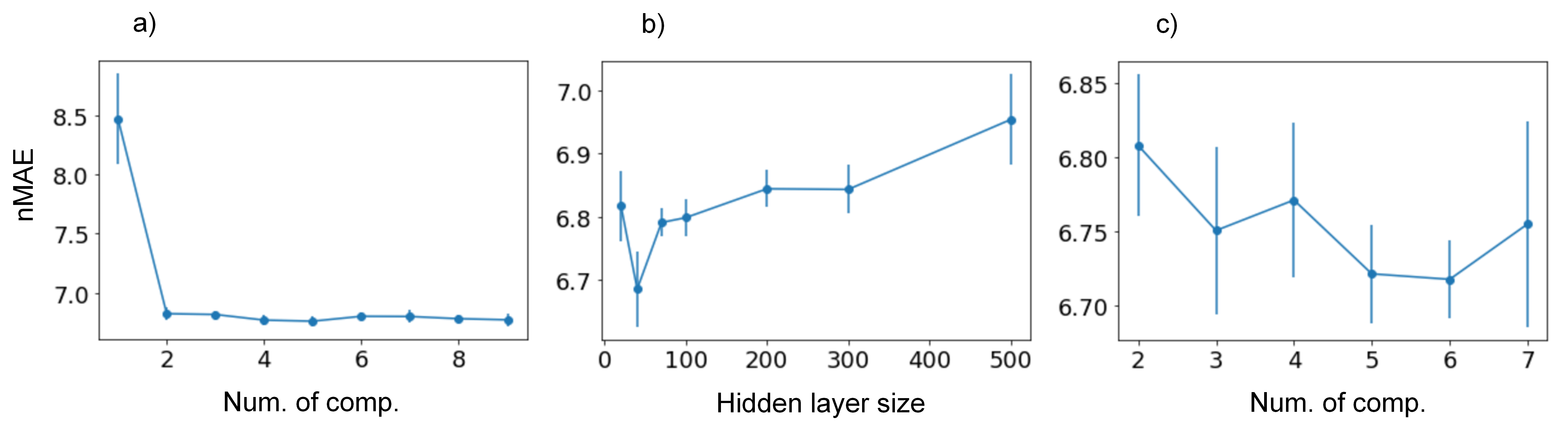
Figure 4: a) nMAE results for variable numbers of positive Gaussian components with hidden layer size 100. b) nMAE results for variable hidden layer sizes with 5 components. c) Refinement of the number of components with hidden layer size 40.

4.5 Ablation study

Our best model configuration (model 1 in Table 1) uses the positive Gaussian distribution combined to the physical model forecasts and the PV system ID as covariates. We first tested replacing the positive Gaussian distribution with the standard Gaussian (model 2) and Student distributions (model 3). We also considered continuous PV system description covariates, instead of the categorical system ID (model 4). The advantage of continuous PV system description covariates is to open the possibility to include new systems without having to learn the model again, which can be highly valuable in production systems. We also test using no PV system covariates at all (model 5), and using only one positive Gaussian component instead of a mixture (model 6). We also consider not using physical model covariates (model 7). This can be of practical interest, as access to ECMWF solar irradiance forecasts, used by the physical model as inputs, is free for research purpose, but requires a subscription for industrial applications. Finally, we tested alternative models: MQCNN [22] (model 8) and FFN [21] (model 9). Physical and system ID covariates were used when possible (with MQCNN, thus comparing to model 1), and ignored otherwise (with FFN, thus rather comparing to model 7).

4.6 Results and interpretation

Results are given in Table 1. In [2], skill scores are computed using a 24h persistence model, adjusted according to the clear sky PV power for the day under consideration. This is a common baseline in the solar energy domain [13]. In this paper, we rather consider that the physical model is the baseline against which our results have to be evaluated. So we use 24h physical model covariates as $\hat{\mathbb{Z}}_{\text{ref}}$ in Equation (8) for computing skill scores presented in Table 1. This is a stronger baseline for skill score computation, as it was shown to significantly outperform persistence forecasts [1]. In this experimental section, this means that a model with a skill score lower than 0 is not able to beat the covariates it is given among its inputs.

ID	Description	nRMSE (%)	nMAE (%)	Skill (%)	CRPS (-)
Baseline
-	Physical model	11.396	7.958	-	-
Models
1	Best model	$\mathbb{10.808(\pm 0.082)}$	$\mathbb{6.707(\pm 0.069)}$	15.72	$\mathbb{4.816(\pm 0.048)}$
2	w/ Gaussian	$10.950(\pm 0.031)$	$6.844(\pm 0.070)$	14.00	$4.897(\pm 0.048)$
3	w/ Student	$10.928(\pm 0.082)$	$6.841(\pm 0.047)$	14.04	$4.916(\pm 0.039)$
4	wo/ system ID	$11.127(\pm 0.102)$	$6.966(\pm 0.049)$	12.47	$5.007(\pm 0.038)$
5	wo/ system	$11.461(\pm 0.100)$	$7.292(\pm 0.067)$	8.37	$5.278(\pm 0.050)$
	wo/ mixture,
6	wo/ system	$11.547(\pm 0.042)$	$7.711(\pm 0.017)$	3.10	$5.676(\pm 0.024)$
7	wo/ physical	$14.203(\pm 0.106)$	$9.333(\pm 0.053)$	-17.28	$6.577(\pm 0.032)$
8	MQCNN [22]	$11.040(\pm 0.101)$	$7.249(\pm 0.031)$	8.91	$5.259(\pm 0.024)$
	FFN [21]
	wo/ system,
9	wo/ physical	$14.687(\pm 0.069)$	$10.087(\pm 0.033)$	-26.75	$7.522(\pm 0.037)$

Table 1: nRMSE, nMAE and CRPS test metrics for the range of compared models. The results of the best performing model are bold-faced. Median results and standard deviations are estimated from 6 models trained independently. w/ and wo/ stand for with and without, respectively.

First focusing on the nMAE metric through skill scores, we see that using the positive Gaussian component has a small but significant influence, with skill scores improved by 1.72 and 1.68 points with respect to the Gaussian and Student components, respectively. The performance of model 4 using continuous PV system description features also yields solid performance, with 2.95 points score degradation compared to model 1. We note that the relatively better performance brought by using the system ID as a covariate provides anecdotal evidence supporting the hypothesis formulated in Section 4.3 regarding the imbalance of systems representation in the dataset. The first significant performance gap comes with model 5, which ignores all PV system covariates. Its score is 4.10 points lower than model 4. Then, as could be anticipated from Section 4.4 on hyper-parameters optimization, using a single positive Gaussian component degrades the performance of model 5 by 5.27 additional points. Finally, the largest gap is observed when ignoring the physical model covariates, while keeping the same configuration as model 1 otherwise, with a negative skill score of -17.28%. This shows that the neural model alone is not able to compete with the physical model, and implicitly validates the relevance of the hybrid-physical approach, which aims at building upon physical models with machine learning techniques [4].

Eventually, using MQCNN yields a positive skill score, but degraded by 6.81 points with respect to model 1. Also, using FFN degrades the results of model 7, its closest variant in our ablation study in terms of available input data, by 9.47 points. This validates our design based on DeepAR and our positive Gaussian component.

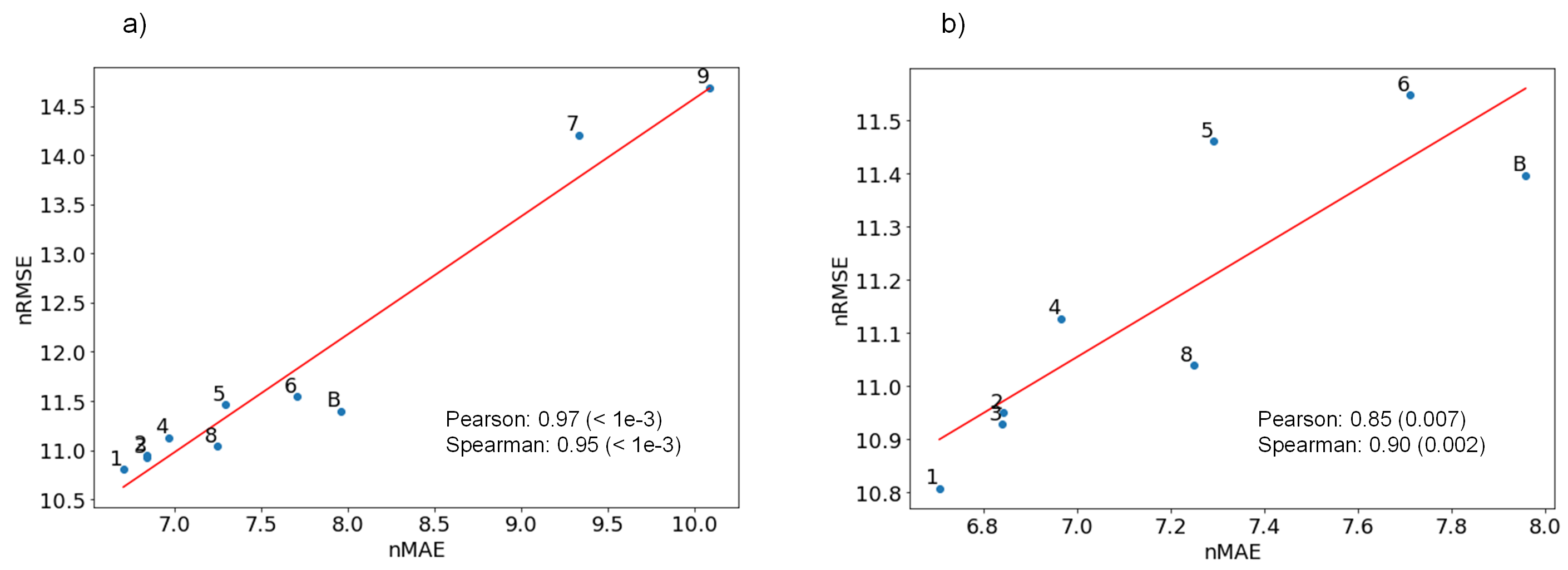
Figure 5: Illustration of the relationship between nMAE and nRMSE metrics (a), also magnified after excluding outlying models 7 and 9 from the representation (b). B stands for the baseline physical model. Red lines are the result of a linear regression of the points in the graph, reported along with Pearson and Spearman correlation coefficients.

Figure 5 illustrates the relationships between nMAE and nRMSE. First we see that the two models which do not use physical model covariates are outlying (Figure 5a), and thus have an important leverage on any correlation analysis. Excluding them indeed has a significant effect on the regression line and computed coefficients (Figure 5b), even if the correlation remains high and significant. Models below the regression line tend to have their nRMSE lower than would be expected according to their nMAE. All models using the system ID (1, 2, 3 and 8) are in this situation, as well as the physical model baseline. This means that in some production context which would favor nRMSE as prime metric, using the system ID as a covariate is preferable. As a side note, we also computed the analysis shown in Figure 5 between nMAE and CRPS metrics; all correlation coefficients were then highly significant and beyond 0.96, even when excluding outlying models 7 and 9. This means that in our experiments, nMAE and CRPS were almost perfectly correlated. Reporting specifically about CRPS would therefore not bring significant added value.

As alternative designs, we considered using unscaled physical model covariates (i.e. not scaling them along with $\mathbb{z}$ values as described in Section 4.1), and using the weighted sampling scheme described in [5], which samples training examples with frequency proportional to the magnitude of $\mathbb{z}$ values. We did not report results with these alternative designs as they brought systematic degradation to the performance. We also tried to use both types of system description covariates (i.e., system ID and continuous description features) simultaneously, but this led to a slight degradation compared to the respective model using only the system ID covariate. This is expected, as the system ID alone already encodes system diversity. In addition, as we will see in the next section, continuous system description features may reflect the system setup in a biased way, which could explain for the slight degradation in performance observed in Table 1.

5 Discussion and qualitative examples

We first emphasize that the contributions highlighted in the introduction are distributed throughout the paper, not only in terms of theoretical contributions in Section 3, which are arguably modest, as we position our work as an application, but also in our analysis of the related work, notably positioning hybrid-physical approaches as a special case in the context of neural-network based time series forecasting in Section 2.2. We also highlight practical contributions on data preprocessing, training and validation procedures in Sections 2.2 and 4.3 which will enable the transfer of the work to the DSO.

In the previous section we evaluated our proposed models using global metrics. In this section, we aim at providing more detailed insight into our results by analyzing model performance at the system level. The displayed examples were obtained using the best performing model (i.e. model 1 in Table 1). First we compute per-sample nMAE metrics for the test set, group them according to their associated system ID, and rank the systems according to the difference between model 1 and the physical model nMAE. In other words, the higher a system is in this ranking, the model 1 outperforms the physical model for this system. For all but 1 system over 119, model 1 performs better than the baseline. We first consider the worst case system 68.

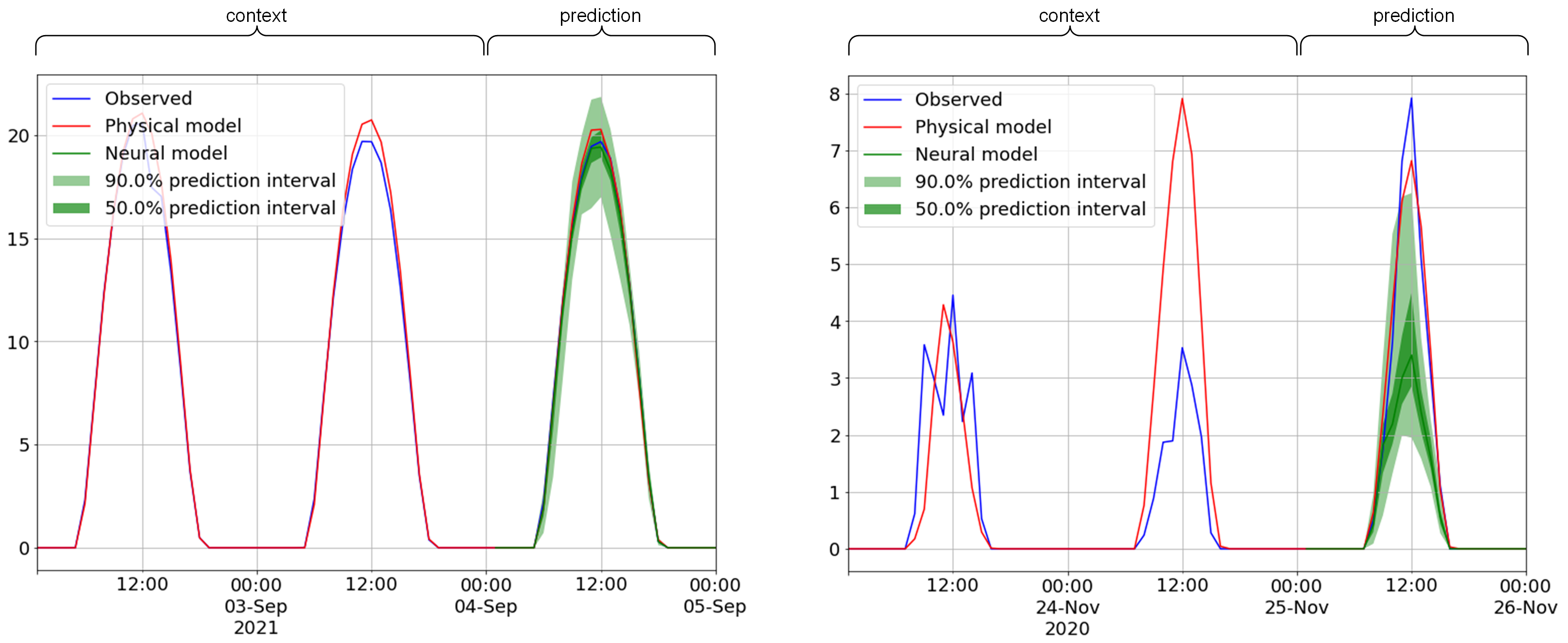
Figure 6: Two test samples associated to system 68. Prediction intervals are displayed using green shades. The observations and 24h physical model forecasts of the context interval are prepended.

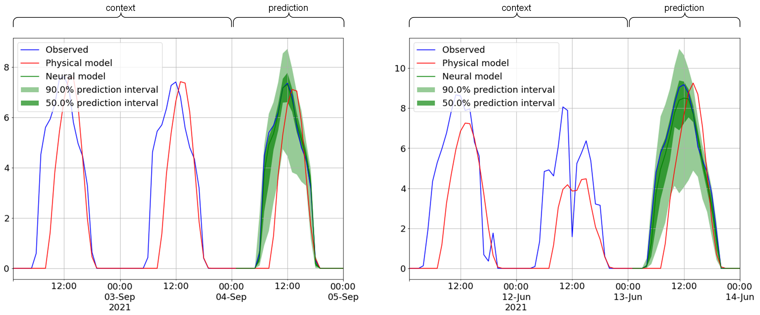
Figure 7: Two test samples associated to system 44. Prediction intervals are displayed using green shades. The observations and 24h physical model forecasts of the context interval are prepended.

On the l.h.s. of Figure 6, we display the sample of this system among the lowest nMAE with the DeepAR model. This is a typical clear day example, where the prediction is fairly easy for the neural model. We note that for this instance, forecasts stick more closely to the observations curve than the baseline. The prediction intervals are naturally tight, reflecting the high confidence of the neural model in this case. On the r.h.s. of Figure 6, for the same system, we display a sample for which the difference between the two models is among the largest. In this case, DeepAR is not able to keep up with the sudden peak of PV power. The 24h physical model covariate somehow informed on this peak, but this information was not used by model 1, which acted conservatively regarding the observations in the context interval.

In Figure 7, we consider samples from system 44. This system is the third best of our ranking, and has been identified as problematic for the physical model because of a double-pitched roof, not reflected by the system description features [2]. On both sides of Figure 7, the systematic shift of the PV performance model is clearly visible. We also see that model 1 is able to completely ignore this shift, and come up with sensible forecasts. The figure also shows how the prediction intervals are tighter when the PV production is stable through days (l.h.s.), and broader when the weather seems more unstable (r.h.s.).

6 Conclusion

Eventually, we are able to improve power forecasts obtained from an already strong physical PV performance model. With an ablation study and model comparisons, our experiments highlight the best working configuration, which uses the PV performance model forecasts as covariates, a mixture of positive Gaussians as output distribution, and a static categorical covariate reflecting the associated system ID. The positive Gaussian output allows to deal effectively with the bell-shaped data profile typical of solar energy applications, and the system ID feature allows to model local effects which went previously unnoticed with the physical PV performance model alone.

In future work, we plan to refine and explore novel neural model designs. For example, quantile regression methods more recent than [22] will be explored. Also, we will further investigate how to deal with novel systems being added to the grid without having to retrain the full model. We saw that using system description features is an effective fallback, but these features do not account for local effects such as a double-pitched roof, so they remain suboptimal. We will also consider longer forecasting intervals (e.g. day-ahead and 2 days ahead).

Despite visible success, models trained for this work tended to overfit, and relied critically on early stopping. This is mostly due to our measures taken to prevent data leakage: when segmenting 2 years of data at the day scale, despite all our measures, training and test sets are unlikely to be identically distributed. We addressed this problem in the most straightforward and conservative way, but it seems related to the domain shift problem characterized by the domain adaptation literature [43]. Adapting contributions from this area to the peculiarities of our application is left for future work.

6.1 Acknowledgements

This research was funded by the Luxembourg National Research Fund (FNR) in the framework of the FNR BRIDGES Project CombiCast with grant number
(BRIDGES18/IS/12705349/Combi-Cast). Furthermore, the authors would like to thank our partner Electris (a brand of Hoffmann Frères Energie et Bois s.à r.l.), for their trust, the very supportive partnership throughout the whole project duration, and their contribution to the common project, financially as well as in terms of manpower and data.

6.2 Data Availability

The datasets analysed during the current study are not publicly available due to being the property of Electris. A sample may be provided by contacting the corresponding author on reasonable request, without any guarantees.

6.3 Declarations

6.3.1 Conflicts of interest

All authors declare that they have no conflicts of interest.

References

- \bibcommenthead
- [1] Koster, D., Minette, F., Braun, C. & O’Nagy, O. Short-term and regionalized photovoltaic power forecasting, enhanced by reference systems, on the example of Luxembourg. Renewable Energy 132, 455–470 (2019).
- [2] Koster, D., Fiorelli, D., Bruneau, P. & Braun, C. Single-Site Forecasts for 130 Photovoltaic Systems at Distribution System Operator Level, Using a Hybrid-Physical Approach, to Improve Grid-Integration and Enable Future Smart-Grid Operation. Solar RRL n/a, 2200652 (2022).
- [3] Hochreiter, S. & Schmidhuber, J. Long short-term memory. Neural Computation 9, 1735–1780 (1997).
- [4] Antonanzas, J. et al. Review of photovoltaic power forecasting. Solar Energy 136, 78–111 (2016).
- [5] Salinas, D., Flunkert, V., Gasthaus, J. & Januschowski, T. DeepAR: Probabilistic forecasting with autoregressive recurrent networks. International Journal of Forecasting 36, 1181–1191 (2020).
- [6] Blaga, R. et al. A current perspective on the accuracy of incoming solar energy forecasting. Progress in energy and combustion science 70, 119–144 (2019).
- [7] Molteni, F., Buizza, R., Palmer, T. N. & Petroliagis, T. The ECMWF Ensemble Prediction System: Methodology and validation. Quarterly Journal of the Royal Meteorological Society 122, 73–119 (1996).
- [8] Yang, D. Choice of clear-sky model in solar forecasting. Journal of Renewable and Sustainable Energy 12, 026101 (2020).
- [9] Inman, R. H., Pedro, H. T. C. & Coimbra, C. F. M. Solar forecasting methods for renewable energy integration. Progress in Energy and Combustion Science 39, 535–576 (2013).
- [10] Bruneau, P. & Boudet, L. Huang, T., Zeng, Z., Li, C. & Leung, C.-S. (eds) Bayesian Variable Selection in Neural Networks for Short-Term Meteorological Prediction. (eds Huang, T., Zeng, Z., Li, C. & Leung, C.-S.) International Conference on Neural Information Processing, 289–296 (Springer Berlin Heidelberg, 2012).
- [11] Elsinga, B. & van Sark, W. Short-term peer-to-peer solar forecasting in a network of photovoltaic systems. Applied Energy 206, 1464–1483 (2017).
- [12] Lonij, V. P. A., Brooks, A. E., Cronin, A. D., Leuthold, M. & Koch, K. Intra-hour forecasts of solar power production using measurements from a network of irradiance sensors. Solar Energy 97, 58–66 (2013).
- [13] Pedro, H. T. C. & Coimbra, C. F. M. Assessment of forecasting techniques for solar power production with no exogenous inputs. Solar Energy 86, 2017–2028 (2012).
- [14] Hyndman, R. J. & Khandakar, Y. Automatic Time Series Forecasting: The forecast Package for R. Journal of Statistical Software 27, 1–22 (2008).
- [15] Shenstone, L. & Hyndman, R. J. Stochastic models underlying Croston’s method for intermittent demand forecasting. Journal of Forecasting 24, 389–402 (2005).
- [16] Seeger, M. W., Salinas, D. & Flunkert, V. Lee, D. D., Sugiyama, M., Luxburg, U. v., Guyon, I. & Garnett, R. (eds) Bayesian Intermittent Demand Forecasting for Large Inventories. (eds Lee, D. D., Sugiyama, M., Luxburg, U. v., Guyon, I. & Garnett, R.) Advances in Neural Information Processing Systems, Vol. 29 (2016).
- [17] Cho, K., Van Merriënboer, B., Bahdanau, D. & Bengio, Y. Wu, D., Carpuat, M., Carreras, X. & Vecchi, E. M. (eds) On the properties of neural machine translation: Encoder-decoder approaches. (eds Wu, D., Carpuat, M., Carreras, X. & Vecchi, E. M.) Workshop on Syntax, Semantics and Structure in Statistical Translation, 103–111 (2014).
- [18] Abadi, M. et al. TensorFlow: Large-scale machine learning on heterogeneous systems (2015). URL https://www.tensorflow.org/.
- [19] Chen, T. et al. MXNet: A Flexible and efficient machine learning library for heterogeneous distributed systems (2015). https://arxiv.org/abs/1512.01274.
- [20] Shi, X. et al. Cortes, C., Lawrence, N. D., Lee, D. D., Sugiyama, M. & Garnett, R. (eds) Convolutional LSTM Network: A Machine Learning Approach for Precipitation Nowcasting. (eds Cortes, C., Lawrence, N. D., Lee, D. D., Sugiyama, M. & Garnett, R.) Advances in Neural Information Processing Systems, Vol. 28 (2015).
- [21] Bebis, G. & Georgiopoulos, M. Feed-forward neural networks. IEEE Potentials 13, 27–31 (1994).
- [22] Wen, R., Torkkola, K., Narayanaswamy, B. & Madeka, D. Anava, O., Khaleghi, A., Kuznetsov, V. & Yang, S. (eds) A Multi-Horizon Quantile Recurrent Forecaster. (eds Anava, O., Khaleghi, A., Kuznetsov, V. & Yang, S.) NIPS Time Series Workshop (2018).
- [23] Gasthaus, J. et al. Chaudhuri, K. & Sugiyama, M. (eds) Probabilistic Forecasting with Spline Quantile Function RNNs. (eds Chaudhuri, K. & Sugiyama, M.) International Conference on Artificial Intelligence and Statistics, 1901–1910 (2019).
- [24] Gneiting, T., Raftery, A. E., Westveld, A. H. & Goldman, T. Calibrated Probabilistic Forecasting Using Ensemble Model Output Statistics and Minimum CRPS Estimation. Monthly Weather Review 133, 1098–1118 (2005).
- [25] Stock, J. H. & Watson, M. W. in Dynamic factor models, factor-augmented vector autoregressions, and structural vector autoregressions in macroeconomics (eds Taylor, J. B. & Uhlig, H.) Handbook of macroeconomics Ch. 2, 415–525 (Elsevier, 2016).
- [26] Salinas, D., Bohlke-Schneider, M., Callot, L., Medico, R. & Gasthaus, J. High-dimensional multivariate forecasting with low-rank Gaussian Copula Processes. Advances in Neural Information Processing Systems 32 (2019).
- [27] Abdel-Nasser, M. & Mahmoud, K. Accurate photovoltaic power forecasting models using deep LSTM-RNN. Neural Computing and Applications 31, 2727–2740 (2019).
- [28] Wang, F. et al. A day-ahead PV power forecasting method based on LSTM-RNN model and time correlation modification under partial daily pattern prediction framework. Energy Conversion and Management 212, 112766 (2020).
- [29] Thaker, J. & Höller, R. A Comparative Study of Time Series Forecasting of Solar Energy Based on Irradiance Classification. Energies 15, 2837 (2022).
- [30] Zou, H. & Hastie, T. Regularization and variable selection via the elastic net. Journal of Royal Statistical Society 67, 301–320 (2005).
- [31] Suhartono, S., Rahayu, S., Prastyo, D. & Wijayanti, D. Hybrid model for forecasting time series with trend, seasonal and calendar variation pattern. Journal of Physics: Conference Series 67, 012160 (2017).
- [32] Cao, J. & Lin, X. Study of hourly and daily solar irradiation forecast using diagonal recurrent wavelet neural networks. Energy Conversion and Management 49, 1396–1406 (2008).
- [33] Rasul, K., Seward, C., Schuster, I. & Vollgraf, R. Meila, M. & Zhang, T. (eds) Autoregressive Denoising Diffusion Models for Multivariate Probabilistic Time Series Forecasting. (eds Meila, M. & Zhang, T.) ICML, 8857–8868 (2021).
- [34] Park, Y. et al. Ruiz, F. J. R., Dy, J. G. & Meent, J.-W. v. d. (eds) Learning Quantile Functions without Quantile Crossing for Distribution-free Time Series Forecasting. (eds Ruiz, F. J. R., Dy, J. G. & Meent, J.-W. v. d.) International Conference on Artificial Intelligence and Statistics, 8127–8150 (2022).
- [35] Benidis, K. et al. Deep Learning for Time Series Forecasting: Tutorial and Literature Survey. ACM Computing Surveys 55, 1–36 (2023).
- [36] Bergmeir, C. & Benítez, J. M. On the use of cross-validation for time series predictor evaluation. Information Sciences 191, 192–213 (2012).
- [37] Geman, S., Bienenstock, E. & Doursat, R. Neural Networks and the Bias/Variance Dilemma. Neural Computation 4, 1–58 (1992).
- [38] Alexandrov, A. et al. GluonTS: Probabilistic and Neural Time Series Modeling in Python. Journal of Machine Learning Research 21, 1–6 (2020). URL http://jmlr.org/papers/v21/19-820.html.
- [39] Devroye, L. Nonuniform Random Variate Generation. Handbooks in Operations Research and Management Science 13, 83–121 (2006).
- [40] Lorenz, E. et al. Comparison of global horizontal irradiance forecasts based on numerical weather prediction models with different spatio-temporal resolutions. Progress in Photovoltaics 24, 1626–1640 (2016).
- [41] Yang, D. & Kleissl, J. Summarizing ensemble NWP forecasts for grid operators: Consistency, elicitability, and economic value. International Journal of Forecasting (2022).
- [42] Lauret, P., Voyant, C., Soubdhan, T., David, M. & Poggi, P. A benchmarking of machine learning techniques for solar radiation forecasting in an insular context. Solar Energy 112, 446–457 (2015).
- [43] Redko, I., Morvant, E., Habrard, A., Sebban, M. & Bennani, Y. Advances in domain adaptation theory (Elsevier, London, 2019).