On the convergence analysis of the decentralized projected gradient descent

Abstract.

In this work, we are concerned with the decentralized optimization problem:

$$\min_{x\in\Omega}~{}f(x)=\frac{1}{n}\sum_{i=1}^{n}f_{i}(x),$$

where $\Omega\subset\mathbb{R}^{d}$ is a convex domain and each $f_{i}:\Omega\rightarrow\mathbb{R}$ is a local cost only known to agent $i$. A fundamental algorithm is the decentralized projected gradient method (DPG) given by

$$x_{i}(t+1)=\mathcal{P}_{\Omega}\Big{[}\sum^{n}_{j=1}w_{ij}x_{j}(t)-\alpha(t)\nabla f_{i}(x_{i}(t))\Big{]}$$

where $\mathcal{P}_{\Omega}$ is the projection operator to $\Omega$ and $\{w_{ij}\}_{1\leq i,j\leq n}$ are communication weight among the agents. While this method has been widely used in the literatures, its sharp convergence property has not been established well so far, except for the special case $\Omega=\mathbb{R}^{n}$. This work establishes new convergence estimates of DPG when the aggregate cost $f$ is strongly convex and each function $f_{i}$ is smooth. If the stepsize is given by constant $\alpha(t)\equiv\alpha>0$ and suitably small, we prove that each $x_{i}(t)$ converges to an $O(\sqrt{\alpha})$-neighborhood of the optimal point. In addition, we take a one-dimensional example $f_{i}$ and prove that the point $x_{i}(t)$ converges to an $O(\alpha)$-neighborhood of the optimal point. Also, we obtain convergence estimates for decreasing stepsizes. Numerical experiments are also provided to support the convergence results.

1. Introduction

Let us consider a multi-agent system with $n$ agents that form a connected network and cooperatively solve the following constrained optimization problem:

$$\min_{x\in\Omega}f(x)=\frac{1}{n}\sum^{n}_{i=1}f_{i}(x),$$ (1.1)

where $f_{i}:\Omega\rightarrow\mathbb{R}$ is a local cost function only known to agent $i\in\mathcal{V}=\{1,2,\cdots,m\}$, and $\Omega\subset\mathbb{R}^{d}$ denotes a common convex closed set. This problem arises in many applications like engineering problems [6, 8], signal processing [3, 24] and machine learning problems [4, 12, 25]. We consider the decentralized projected gradient (DPG) algorithm [20, 26] given by

$$x_{i}(t+1)=\mathcal{P}_{\Omega}\bigg{[}\sum^{n}_{j=1}w_{ij}x_{j}(t)-\alpha(t)\nabla f_{i}({x}_{i}(t))\bigg{]},$$ (1.2)

where $P_{\Omega}$ denotes the projection of a vector $y\in\mathbb{R}^{d}$ onto the domain $\Omega$:

$$\mathcal{P}_{\Omega}[y]=\arg\min_{x\in\Omega}\|x-y\|.$$

The nonnegative weight scalars $w_{ij}$ are related to the communication pattern among agents in (1.1) (see section 2 for the detail). This algorithm is studied for various settings containing stochastic distributed optimization [2, 19, 22, 26], event-triggered communication [15, 17], and online problems [1, 7, 14]. In addition, the algorithm has been widely used as a backbone for developing various algorithms such as the decentralized TD learning for the multi-agent reinforcement learning [10] and distributed model predictive control [16]. Despite of its wide applications, the convergence property of the algorithm (1.2) has not been established well due to the difficulty of handling the projection operator $P_{\Omega}$ in the convergence analysis.

When $\Omega=\mathbb{R}^{n}$, the algorithm (1.2) becomes the unconstrained decentralized gradient descent as given by

$$x_{i}(t+1)=\sum^{n}_{j=1}w_{ij}x_{j}(t)-\alpha(t)\nabla f_{i}({x}_{i}(t)).$$ (1.3)

The convergence estimates of (1.3) have been established well in the previous works [20, 21, 27, 9]. For a constant stepsize, Nedić-Ozdaglar [20] showed that the sequence converges to an $O(\alpha)$-neighborhood of the optimal set. In the earlier works [20, 21], the convergence results were established under the assumption that the gradient $\nabla f_{i}$ has a uniform bound for $1\leq i\leq n$. Also, the sequence converges to the optimal set for suitable decreasing stepsize. In the recent work, [27], the convergence result was established for local cost functions with Lipschitz continuous gradient instead of the uniform boundedness assumption on the gradient. It was shown that the sequence with constant stepsize $\alpha(t)\equiv\alpha>0$ (smaller than a specific value) converges to an $O(\alpha)$-neighborhood of the optimal point exponentially fast if the global cost function is strongly convex. This result was extended [9] to the case with decreasing stepsize of the form $\alpha(t)=c/(t+w)^{\alpha}$ for $0<\alpha\leq 1$.

We mention that, if $\Omega\neq\mathbb{R}^{n}$, the convergence analysis for (1.2) becomes more challenging due to the projection operator. In the original works [26, 11, 18], the convergence results of (1.2) were established under the assumption that the gradient $\nabla f_{i}$ has a uniform bound for $1\leq i\leq n$. The work [18] obtained the convergence rate $O(1/\sqrt{t})$ when the stepsize is chosen as $\alpha(t)=c/t$ for a suitable range of $c>0$.

The uniform boundedness of the gradient assumption was replaced by the $L$-smoothness property in the work [17]. For the algorithm (1.2) with constant stepsize $\alpha>0$, the authors showed that there exists a uniform bound $D>0$ of the gradients $\|\nabla f_{i}(x_{t})\|$ for all $t\geq 0$ and $1\leq i\leq n$. In addition, the following convergence estimate was obtained:

$$\begin{split}\|x_{i}(t+1)-x_{*}\|&\leq(1-c\alpha)^{t+1}\|\bar{x}_{0}-x_{*}\|+\beta^{t+1}\|x_{0}\|+\frac{2\alpha D}{1-\beta}\\ &\quad+\sum_{i=0}^{t}(1-c\alpha)^{t-i}\Big{(}\alpha L\gamma_{i}+\frac{\alpha D}{\sqrt{n}}\Big{)},\end{split}$$ (1.4)

where $x_{*}$ denotes an optimizer of (1.1) and $\gamma_{i}=\beta^{i}\|x_{0}\|+\frac{2\alpha D}{1-\beta}$. The above mentioned results are summarized in Table 1.

We remark that the right hand side of (1.4) involves the following term

$$\sum_{i=0}^{t}(1-c\alpha)^{t-i}\frac{\alpha D}{\sqrt{n}}=\frac{D}{c\sqrt{n}}\Big{[}1-(1-c\alpha)^{t+1}\Big{]},$$

which converges to $\frac{D}{c\sqrt{n}}$ as the number of iterations $t$ goes to infinity. This limit is independent of the stepsize $\alpha>0$. Therefore, the right hand side of above estimate (1.4) in the limit $t\rightarrow\infty$ involves the term $\frac{D}{c\sqrt{n}}$. However, this convergence estimate is not as strong as the estimate for (1.3) by the work in [27] which showed that the sequence of (1.3) with constant stepsize $\alpha(t)\equiv\alpha>0$ (below a certain threshold) converges exponentially fast to an $O(\alpha)$-neighborhood of the optimal point. Having these results, it is natural to pose the following question:

Question: Does the algorithm (1.2) with constant stepsize $\alpha>0$ converges to the optimizer $x_{*}$ up to an $O(\alpha^{c})$ error for some $c>0$?

It is worth mentioning that this fundamental question is still open and has not been resolved as of now. In this work, we show that the convergence property of this question holds with $c=1/2$ if the total cost function $f$ is $\mu$ strongly convex and each local cost function $f_{i}$ is $L_{i}$ smooth. In addition, we exhibit a concrete example where the property holds with $c=1$.

To explain the difficulty in the convergence analysis of (1.2) compared to the case $\Omega=\mathbb{R}^{n}$, we note that averaging (1.3) gives

$$\bar{x}(t+1)=\bar{x}(t)-\frac{\alpha(t)}{n}\sum_{i=1}^{n}\nabla f_{i}(x_{i}(t)),$$ (1.5)

where $\bar{x}(t)=\frac{1}{n}\sum_{i=1}^{n}x_{i}(t)$. Then, if the stepsize is set to $\alpha\leq\frac{2}{\mu+L}$, one can obtain the following inequality:

$$\begin{split}\|\bar{x}(t+1)-x_{*}\|&\leq\Big{(}1-\frac{\mu L}{\mu+L}\alpha\Big{)}\|\bar{x}(t)-x_{*}\|+\frac{L\alpha}{n}\sum_{i=1}^{n}\|x_{i}(t)-\bar{x}(t)\|,\end{split}$$

when $f$ is $\mu$-strongly convex and each $f_{i}$ is $L$-smooth. This inequality is a major ingredient in the convergence estimate of (1.3) in the work [27, 9], but the identity (1.5) no longer holds for (1.2) due to the projection. Instead, we proceed to obtain a sequential estimate of the quantity

$$\sum_{i=1}^{N}\|x_{i}(t)-x_{*}\|^{2},$$

which enables us to offset the projection operator efficiently using the contraction property of the projection operator (see Section 4 for the detail). As a result, we obtain a convergence result up to an error $O(\sqrt{\alpha})$. We point out that our result is obtained for (1.2) with the projection operator to an arbitrary convex set $\Omega\subset\mathbb{R}^{d}$ which is possibly unbounded.

	Cost	Smooth	Learning rate	Regret	Rate
[26]	C	$\|\nabla f_{i}\|_{{\infty}}<\infty$	$\sum_{t=1}^{\infty}\alpha(t)=\infty$ $\sum_{t=1}^{\infty}\alpha(t)^{2}<\infty$	$\|x_{i}(t)-x_{*}\|$	$o(1)$
[11]	C	$\|\nabla f_{i}\|_{{\infty}}<\infty$	$\alpha(t)=\frac{c}{t^{\alpha}}$	$\min_{1\leq k\leq n}$ $f(x_{k}(t))-f_{*}$	$O(\frac{1}{n^{\alpha}})$ if $0<\alpha<\frac{1}{2}$ $O(\frac{\log n}{\sqrt{n}})$ if $\alpha=\frac{1}{2}$ $O(\frac{1}{n^{1-\alpha}})$ if $\frac{1}{2}<\alpha<1$
[18]	SC	$\|\nabla f_{i}\|_{{\infty}}<\infty$	$\alpha(t)=c/t$	$\|x_{i}(t)-x_{*}\|$	$O(1/\sqrt{t})$
[17]	SC	L-smooth	$\alpha(t)\equiv\alpha$	$\|x_{i}(t)-x_{*}\|$	$O(e^{-ct})+O(\sqrt{\alpha})+O(\frac{D}{\sqrt{n}})$
This work	SC	L-smooth	$\alpha(t)\equiv\alpha$	$\|\bar{x}(t)-x_{*}\|$	$O(e^{-ct})+O(\sqrt{\alpha})$
This work	Specific example	L-smooth	$\alpha(t)\equiv\alpha$	$\|\bar{x}(t)-x_{*}\|$	$O(e^{-ct})+O({\alpha})$
This work	SC	L-smooth	$\alpha(t)=\frac{c}{t^{\alpha}}$	$\|\bar{x}(t)-x_{*}\|$	$O(\frac{1}{t^{\alpha/2}})$ if $0<\alpha<1$ $O(\frac{1}{t^{\mu_{0}}})$ if $\alpha=1$

Table 1. Convergene results for DPG. Here C and SC mean that convex and $\mu$-strongly convex, respectively.

The rest of this paper is organized as follows. In Section 2 we introduce some assumptions and state our main results. In Section 3, we recall some preliminary results and give some useful estimatest that we will use throughout the paper. Section 4 is devoted to obtaining sequential estimates for the algorithm. Based on these sequential estimates, we establish the uniform boundedness of the sequence in Section 5. Then we obtain consensus estimates in Section 6 and prove the main convergence results in Section 7. In Section 8, we derive an optimal convergence result for a specific example in dimension one. Finally, we perform numerical experiments to support the main theorems in Section 9.

2. Assumptions and main results

In this section, we state the assumptions on the total and local cost functions in (1.1) and communication patterns among agents. Then we give the main results of this paper. We are interested in (1.1) when the local cost functions and the total cost functions satisfy the following strong convexity and smoothness assumption.

Assumption 1.

For each $i\in\{1,\cdots n\}$, the local cost function $f_{i}$ is $L_{i}$-smooth for some $L_{i}>0$, i.e., for any $x,y\in\Omega$ we have

$$\|\nabla f_{i}(x)-\nabla f_{i}(y)\|\leq L_{i}\|x-y\|\quad\forall~{}x,y\in\Omega.$$

We set $L=\max_{1\leq i\leq n}L_{i}$. Then the total cost function $f(\cdot)=\frac{1}{n}\sum^{n}_{i=1}f_{i}(\cdot)$ is $L$-smooth.

Throughout the paper, we use $\|\cdot\|$ to denote the euclidean norm.

Assumption 2.

The total cost function $f(\cdot)=\frac{1}{n}\sum^{n}_{i=1}f_{i}(\cdot)$ is $\mu$-strongly convex for some $\mu>0$, i.e., for any $x,y\in\Omega$, we have

$$f(y)\geq f(x)+(y-x)\nabla f(x)+\frac{\mu}{2}\|y-x\|^{2}.$$

Under this assumption, the function $f$ has a unique optimizier $x_{*}\in\Omega$. In decentralized optimization, a local agent informs its own information to other agents relying on shared communication networks which are characterized by an undirected graph $\mathcal{G}=(\mathcal{V},\mathcal{E})$, where each node in $\mathcal{V}$ represents an agent, and each edge $\{i,j\}\in\mathcal{E}$ means that $i$ can send messages to $j$. The graph $\mathcal{G}$ is assumed to satisfy the following assumption.

Assumption 3.

The communication graph $\mathcal{G}$ is fixed and connected.

We define the mixing matrix $W=[w_{ij}]_{1\leq i,j\leq n}$ as follows. The nonnegative weight $w_{ij}$ is given for each communication link $\{i,j\}\in\mathcal{E},$ where $w_{ij}\neq 0$ if $\{i,j\}\in\mathcal{E}$ and $w_{ij}=0$ if $\{i,j\}\notin\mathcal{E}$. In this paper, we make the following assumption on the mixing matrix $W$.

Assumption 4.

The mixing matrix $W=\{w_{ij}\}_{1\leq i,j\leq n}$ is symmetric and doubly stochastic. The network is strongly connected and the weight matrix $W$ satisfies $\textrm{null}(I-W)=\textrm{span}\{1_{n}\}$.

Without loss of generality, we arrange the eigenvalues of $W$ to satisfy

$$1=|\lambda_{1}(W)|>|\lambda_{2}(W)|\geq\cdots\geq|\lambda_{n}(W)|\geq 0.$$

It is well-known that we have $\beta:=|\lambda_{2}(W)|<1$ under Assumption 4. Furthermore, we have the following lemma.

Lemma 2.1.

Suppose that the mixing matrix $W$ satisfies the Assumption 4. Then, for any $x=(x_{1},\cdots,x_{n})\in\mathbb{R}^{d\cdot n}$ we have

$$\sum_{i=1}^{n}\Big{\|}\sum_{j=1}^{n}w_{ij}(x_{j}-\bar{x})\Big{\|}^{2}\leq\beta^{2}\sum_{i=1}^{n}\|x_{i}-\bar{x}\|^{2},$$

where $\bar{x}=\frac{1}{n}\sum^{n}_{i=1}x_{i}$.

Proof.

We refer to Lemma 1 in [23]. ∎

2.1. Main Results

In centralized optimization, it is enough to show that the sequence generated by (1.5) converges to the optimal solution of (1.1) since the central coordinate control all agents simultaneously. On the other hand, in decentralized optimization, each agent makes its own sequence and only informs its own information to its neighbor agents. Therefore, we also need to show that each sequence generated by (1.2) converges to the same point, in which case we say the consensus is achieved. Then we reveal this point converges to the optimal point. Before stating the results, we introduce some constants used to state and prove the results. Let $D:=\max_{1\leq i\leq n}\|\nabla f_{i}(x_{*})\|$. We fix a variable $\delta>0$ such that $(1+\delta)\beta^{2}<1$ and let $\tilde{\beta}:=(1+\delta)\beta^{2}$. Also, we set the following constants

$$c_{1}:=3L^{2}\bigg{(}1+\frac{1}{\delta}\bigg{)},\ c_{2}:=3nD^{2}\bigg{(}1+\frac{1}{\delta}\bigg{)},\ c_{3}:=c_{1}+L^{2},\ c_{4}:=\frac{4L^{2}}{\mu}$$ (2.1)

and denote $\mathbf{x}(t)$, $\bar{\mathbf{x}}(t)$ and $\mathbf{x}_{*}\in\mathbb{R}^{d\cdot n}$ by

$$\begin{split}\mathbf{x}(t)=[x_{1}(t),x_{2}(t)\cdots,x_{n}(t)]^{T},\ \bar{\mathbf{x}}(t)=[\bar{x}(t),\cdots\bar{x}(t)]^{T},\ \mathbf{x}_{*}=[x_{*},\cdots,x_{*}]^{T}.\end{split}$$

where $\bar{x}(t)=\frac{1}{n}\sum^{n}_{i=1}x_{i}(t)$. We note that

$$\|\mathbf{x}(t)-\mathbf{\bar{x}}(t)\|^{2}=\sum^{n}_{i=1}\|x_{i}(t)-\bar{x}(t)\|^{2}\ \text{and}\ \|\mathbf{x}(t)-\mathbf{x}_{*}\|^{2}=n\|\bar{x}(t)-x_{*}\|^{2}.$$

In addition, since $\frac{1}{n}\sum^{n}_{i=1}x_{i}(t)-\bar{x}(t)=0$, it follows directly that for all $t\geq 0$,

$$\|\mathbf{x}(t)-\mathbf{x}_{*}\|^{2}=\|\mathbf{x}(t)-\bar{\mathbf{x}}(t)\|^{2}+\|\bar{\mathbf{x}}(t)-\mathbf{x}_{*}\|^{2}.$$ (2.2)

Now we introduce our results on the projected decentralized gradient descent (1.2). The first result provides the conditions for the uniform boundedness of the sequence $\{x_{i}(t)\}_{t\geq 0}$ in the sense that $\|\mathbf{x}(t)-\mathbf{\bar{x}}(t)\|^{2}$ is uniformly bounded for all $t\geq 0$.

Theorem 2.1.

Suppose that Assumptions 1,3,4 hold. Also, assume that one of the following statements holds true:

1. $\Omega$ is bounded.

2. Each cost $f_{i}$ is convex and the stepsize is constant, i.e., $\alpha(t)\equiv\alpha$, satisfying $\alpha\leq\frac{1+\lambda_{n}(W)}{L}$.

3. Assumption 2 holds. Also the stepsize $\{\alpha(t)\}_{t\geq 0}$ is non-increasing and $\alpha(0)$ satisfies

   $$\alpha(0)<\min\bigg{\{}Z,\frac{\mu}{4c_{1}},\frac{2}{L+\mu}\bigg{\}}.$$

   Here we have set the positive constant $Z$ by

   $$Z:=\frac{1}{2c_{3}}\Big{[}-\Big{(}c_{4}+\frac{\mu}{4}\Big{)}+\sqrt{\Big{(}c_{4}+\frac{\mu}{4}\Big{)}^{2}+4c_{3}(1-\tilde{\beta})}\Big{]}.$$

Then there exists a constant $R>0$ such that

$$\|\mathbf{x}(t)-\mathbf{\bar{x}}(t)\|^{2}\leq R$$

holds for all $t\geq 0$.

The following assumption formulates the above uniform boundedness property:

Assumption 5.

There exists a constant $R>0$ such that

$$\|\mathbf{x}(t)-\mathbf{\bar{x}}(t)\|^{2}\leq R$$

holds for all $t\geq 0$.

Although the result of this assumption is proved in Theorem 2.1, we proposed this assumption because the result may hold for larger ranges of $\alpha(t)$ than that guaranteed by Theorem 2.1. Proving a sharper range of $\alpha(t)$ for the uniform boundedness property would be an interesting future work.

Now we state the consensus and convergence results for (1.2) both for the constant stepsize and decreasing stepsize. We first introduce the following consensus results based on the estimates for the consensus error $\|\mathbf{x}(t)-\mathbf{\bar{x}}(t)\|^{2}$.

Theorem 2.2.

Suppose that Assumptions 1-5 hold. If $\{\alpha(t)\}_{t\geq 0}$ satisfies $\alpha(0)\leq\frac{2}{L+\mu}$, then we have

$$\|\mathbf{x}(t)-\bar{\mathbf{x}}(t)\|^{2}\leq\beta^{t}\|\mathbf{x}(0)-\bar{\mathbf{x}}(0)\|^{2}+\frac{J\alpha(t)^{2}}{(1-\beta)^{2}}.$$

Here for constant stepsize, i.e. $\alpha(t)\equiv\alpha$, we set

$$J:=3(L^{2}R^{2}+nD^{2}).$$

For a decreasing stepsize, we set

$$J:=3(L^{2}R^{2}+nD^{2})\cdot\sup_{s\geq 0}\frac{\alpha(0)^{2}\beta^{s}+\alpha([s/2])^{2}}{\alpha(s)^{2}}.$$

Theorem 2.2 demonstrates that the consensus is reached exponentially up to an $O(\alpha(t))$ error. Next we state the convergence results for the sequence $\{\bar{x}(t)\}_{t\geq 0}$ towards the optimal point. Before stating the results, we introduce the following constants $G_{1}$ and $G_{2}$:

$$\begin{split}G_{1}&=2R\Big{(}\tilde{c}_{3}\alpha(0)^{2}+\tilde{c}_{4}\alpha(0)+\beta\Big{)}\\ G_{2}&=\Big{[}(\tilde{c}_{3}\alpha(0)^{2}+\tilde{c}_{4}\alpha(0)+\beta)\frac{2J^{2}}{(1-\beta)^{2}}+\tilde{c}_{1}R+\tilde{c}_{2}\Big{]},\end{split}$$

where

$$\tilde{c}_{1}:=\frac{3L^{2}}{1-\beta},\ \tilde{c}_{2}:=\frac{3nD^{2}}{1-\beta},\ \tilde{c}_{3}:=\tilde{c}_{1}+L^{2},\ \tilde{c}_{4}:=\frac{4L^{2}}{\mu}.$$

These constants are obtained by setting $\delta=(1-\beta)/\beta$ in the constants of (2.1). The following convergence result holds when the stepsize is given by a constant.

Theorem 2.3.

Suppose that Assumptions 1-5 hold. If the stepsize is given by a constant $\alpha>0$ such that $\alpha\leq\frac{2}{L+\mu}$, then we have

$$\|\bar{\mathbf{x}}(t)-\mathbf{x}_{*}\|^{2}\leq\Big{(}1-\frac{\mu\alpha}{2}\Big{)}^{t}\|\bar{\mathbf{x}}(0)-\mathbf{x}_{*}\|^{2}+\frac{2G_{2}}{\mu}\alpha+\frac{2}{\mu\alpha}\left(\left(1-\frac{\mu\alpha}{2}\right)^{t-1}+\beta^{\frac{t-1}{2}}\right).$$

Theorem 2.3 implies the sequence generated by (1.2) converges to an $O(\sqrt{\alpha})$-neighborhood of the optimal point exponentially fast. We recall from [27] that the sequence of the algorithm (1.2) on the whole space $\mathbb{R}^{d}$ converges to an $O(\alpha)$-neighborhood of $x_{*}$. This naturally leads us to pose the following question.

Question: Is the convergence error $O(\sqrt{\alpha})$ in Theorem 2.3 optimal? or can we improve the convergence error to $O(\alpha)$?

We give a partial answer to this question in Section 8. Precisely, we find a one-dimensional example such that the algorithm (1.2) converges to an $O(\alpha)$ neighborhood of the optimal point.

In the below, we provide the convergence results when the stepsize is given by the decreasing stepsize $\alpha(t)=v/(t+w)^{p}$ for $0<p\leq 1$.

Theorem 2.4.

Suppose that Assumptions 1-5 hold. Let $p\in(0,1)$ and assume that $\alpha(t)=\frac{v}{(t+w)^{p}}$ with $v,w>0$ satisfying

$$\alpha(0)=\frac{v}{w^{p}}\leq\frac{2}{L+\mu}.$$

Then we have

$$\|\bar{\mathbf{x}}(t)-\mathbf{x}_{*}\|^{2}\leq\frac{2eQ\Big{(}\rho G_{1}+G_{2}\Big{)}v}{\mu}([t/2]+w-1)^{-p}+\mathcal{R}_{1}(t)+\mathcal{R}_{2}(t),$$

where $Q=\Big{(}\frac{w+1}{w}\Big{)}^{2p}$, $\rho=\sup_{t\geq 0}\beta^{t}/\alpha(t)^{2}$ and

$$\begin{split}\mathcal{R}_{1}(t)&=e^{-\sum^{t-1}_{s=0}\frac{\mu v}{2(s+w)^{p}}}\|\bar{\mathbf{x}}(0)-\mathbf{x}_{*}\|^{2},\\ \mathcal{R}_{2}(t)&=Q\Big{(}\rho G_{1}+G_{2}\Big{)}v^{2}e^{-\frac{\mu vt}{4(t+w)^{p}}}\sum^{[t/2]-1}_{s=1}\frac{1}{(s+w)^{2p}}.\end{split}$$

In the above result, we easily see that for any fixed $N>0$, there exists a constant $C_{N}>0$ independent of $t\geq 0$ such that

$$\mathcal{R}_{1}(t)+\mathcal{R}_{2}(t)\leq C_{N}t^{-N}.$$

Theorem 2.5.

Suppose that Assumptions 1-5 hold. Let $\alpha(t)=\frac{v}{(t+w)}$ with $v,w>0$ satisfying

$$\alpha(0)=\frac{v}{w}\leq\frac{2}{L+\mu}.$$

Also, choose $v>0$ such that $\mu v/2>1$. Then we have

$$\|\bar{\mathbf{x}}(t)-\mathbf{x}_{*}\|^{2}\leq\left(\frac{w}{t+w}\right)^{\mu v/2}\|\bar{\mathbf{x}}(0)-\mathbf{x}_{*}\|^{2}+\mathcal{R}_{3}(t),$$

where $Q=\Big{(}\frac{w+1}{w}\Big{)}^{2}$, $\rho=\sup_{t\geq 0}\beta^{t}/\alpha(t)^{2}$ and

$$\mathcal{R}_{3}(t)=\frac{Q}{(\mu v/2)-1}\Big{(}\frac{w+1}{w}\Big{)}^{\mu v/2}\frac{\Big{(}\rho G_{1}+G_{2}\Big{)}v^{2}}{(t+w-1)}.$$

3. Preliminary results

In this section, we prepare several estimates which will be used to derive two sequential estimates in the next section. We first study the projection operator $\mathcal{P}_{\Omega}$ in (1.2) defined by

$$\mathcal{P}_{\Omega}[x]=\arg\min_{y\in\Omega}\|y-x\|.$$

This projection operator has the following property:

Lemma 3.1.

Let $\Omega\subset\mathbb{R}^{d}$ be convex and closed.

1. For any $x,y\in\mathbb{R}^{d}$, we have

   $$\|\mathcal{P}_{\Omega}[x]-\mathcal{P}_{\Omega}[y]\|\leq\|x-y\|.$$ (3.1)

2. For any $x\in\mathbb{R}^{d}$ and $y\in\Omega$, we have

   $$\|\mathcal{P}_{\Omega}[x]-y\|\leq\|x-y\|.$$ (3.2)

Proof.

We refer to Theorem 1.5.5 in [13] for the proof of estimate (3.1). Taking $y\in\Omega$ in (3.1) leads to the estimate (3.2). ∎

The following lemma will be used to obtain the sequential estimates in Section 4.

Lemma 3.2.

Let $\Omega\subset\mathbb{R}^{d}$ be convex and closed. Then, for any $x_{1},\cdots,x_{n}\in\mathbb{R}^{d}$, we have

$$\sum^{n}_{i=1}\Bigg{\|}\mathcal{P}_{\Omega}[x_{i}]-\frac{1}{n}\sum^{n}_{j=1}\mathcal{P}_{\Omega}[x_{j}]\Bigg{\|}^{2}\leq\sum^{n}_{i=1}\left\|x_{i}-\frac{1}{n}\sum^{n}_{j=1}x_{j}\right\|^{2}.$$

Proof.

For given $\{a_{i}\}_{i=1}^{n}\subset\mathbb{R}^{d}$, consider the function $F:\mathbb{R}^{d}\rightarrow\mathbb{R}$ defined by

$$F(x)=\sum_{i=1}^{n}\|a_{i}-x\|^{2},$$

This function is minimized when $x=\frac{1}{n}\sum_{i=1}^{n}a_{i}$, and using this we find

$$\sum^{n}_{i=1}\Bigg{\|}\mathcal{P}_{\Omega}[x_{i}]-\frac{1}{n}\sum^{n}_{j=1}\mathcal{P}_{\Omega}[x_{j}]\Bigg{\|}^{2}\leq\sum^{n}_{i=1}\Bigg{\|}\mathcal{P}_{\Omega}[x_{i}]-\mathcal{P}_{\Omega}\bigg{[}\frac{1}{n}\sum^{n}_{j=1}x_{j}\bigg{]}\Bigg{\|}^{2}.$$

Combining this with (3.1), we get the desired inequality. ∎

Lemma 3.3.

Suppose that Assumptions 1 and 2 hold. If $\alpha(t)\leq\frac{2}{L+\mu}$ for all $t\geq 0$, then we have

$$\left\|\bar{x}(t)-x_{*}-\frac{\alpha(t)}{n}\sum^{n}_{i=1}(\nabla f_{i}(\bar{x}(t))-\nabla f_{i}(x_{*}))\right\|^{2}\leq\bigg{(}1-\frac{\mu\alpha(t)}{2}\bigg{)}^{2}\|\bar{x}(t)-x_{*}\|^{2}.$$ (3.3)

Proof.

We expand the left hand side in (3.3) as

$$\|\bar{x}(t)-x_{*}\|^{2}-2\alpha(t)\Big{\langle}\bar{x}(t)-x_{*},\nabla f(\bar{x}(t))-\nabla f(x_{*})\Big{\rangle}+\alpha(t)^{2}\left\|\nabla f(\bar{x}(t))-\nabla f(x_{*})\right\|^{2},$$ (3.4)

where $f(x)=\frac{1}{n}\sum^{n}_{i=1}f_{i}(x).$ Note that $f$ is $L$-smooth and $\mu$-strongly convex by Assumptions 1 and 2, and so we have the following inequality (see e.g., [5, Lemma 3.11]):

$$\Big{\langle}\bar{x}(t)-x_{*},~{}\nabla f(\bar{x}(t))-\nabla f(x_{*})\Big{\rangle}\geq\frac{L\mu}{L+\mu}\|\bar{x}(t)-x_{*}\|^{2}+\frac{1}{L+\mu}\|\nabla f(\bar{x}(t))-\nabla f(x_{*})\|^{2}.$$

Putting the above inequality in (3.4), we get

$$\left\|\bar{x}(t)-x_{*}-\frac{\alpha(t)}{n}\sum^{n}_{i=1}(\nabla f_{i}(\bar{x}(t))-\nabla f_{i}(x_{*}))\right\|^{2}$$

$$\leq\bigg{(}1-\frac{2L\mu\alpha(t)}{L+\mu}\bigg{)}\|\bar{x}(t)-x_{*}\|^{2}+\alpha(t)\bigg{(}\alpha(t)-\frac{2}{L+\mu}\bigg{)}\|\nabla f(\bar{x}(t))-\nabla f(x_{*})\|^{2}.$$

Using the assumption $\alpha(t)\leq\frac{2}{L+\mu}$ and $2L\geq L+\mu$, we then have

$$\begin{split}\left\|\bar{x}(t)-x_{*}-\frac{\alpha(t)}{n}\sum^{n}_{i=1}(\nabla f_{i}(\bar{x}(t))-\nabla f_{i}(x_{*}))\right\|^{2}&\leq\bigg{(}1-\frac{2L\mu\alpha(t)}{L+\mu}\bigg{)}\|\bar{x}(t)-x_{*}\|^{2}\\ &\leq\bigg{(}1-\frac{\mu\alpha(t)}{2}\bigg{)}^{2}\|\bar{x}(t)-x_{*}\|^{2}.\end{split}$$

The proof is done. ∎

Lemma 3.4.

Suppose that Assumption 1 holds. For $(x_{1},\cdots,x_{n})\in\mathbb{R}^{dn}$ and $\bar{x}=\frac{1}{n}\sum_{k=1}^{n}x_{k}$ we have

$$\sum^{n}_{i=1}\|\nabla f_{i}({x}_{i})-\nabla f_{i}(\bar{x})\|^{2}\leq L^{2}\|\mathbf{x}-\bar{\mathbf{x}}\|^{2}$$ (3.5)

and

$$\sum_{i=1}^{n}\Big{\|}\nabla f_{i}({x}_{i})-\frac{1}{n}\sum_{l=1}^{n}\nabla f_{l}({x}_{l})\Big{\|}^{2}\leq 3L^{2}\|\mathbf{x}-\bar{\mathbf{x}}\|^{2}+3L^{2}\|\bar{\mathbf{x}}-\mathbf{x}_{*}\|^{2}+3nD^{2}.$$ (3.6)

Proof.

By Assumption 1, we have

$$\sum^{n}_{i=1}\|\nabla f_{i}({x}_{i})-\nabla f_{i}(\bar{x})\|^{2}\leq L^{2}\sum^{n}_{i=1}\|{x}_{i}-\bar{x}\|^{2},$$

which directly implies (3.5). Next, we prove (3.6). Note that for any $a=(a_{1},\cdots,a_{n})\in\mathbb{R}^{n}$, we have

$$\begin{split}\sum^{n}_{i=1}\left\|a_{i}-\frac{1}{n}\sum^{n}_{l=1}a_{l}\right\|^{2}&=\sum^{n}_{i=1}\left(\|a_{i}\|^{2}-2\left\langle a_{i},\frac{1}{n}\sum^{n}_{l=1}a_{l}\right\rangle+\frac{1}{n^{2}}\left\|\sum^{n}_{l=1}a_{l}\right\|^{2}\right)\\ &=\sum^{n}_{i=1}\|a_{i}\|^{2}+\left(\frac{1}{n^{2}}-\frac{2}{n}\right)\left\|\sum^{n}_{l=1}a_{l}\right\|^{2}\\ &\leq\sum^{n}_{i=1}\|a_{i}\|^{2}.\end{split}$$

Using this, it follows that

$$\begin{split}\sum_{i=1}^{n}\left\|\nabla f_{i}({x}_{i})-\frac{1}{n}\sum_{l=1}^{n}\nabla f_{l}({x}_{l})\right\|^{2}&\leq\sum^{n}_{i=1}\|\nabla f_{i}({x}_{i}(t))\|^{2}.\end{split}$$

By the triangle inequality, one has

$$\|\nabla f_{i}({x}_{i})\|^{2} \leq 3\|\nabla f_{i}({x}_{i})-\nabla f_{i}(\bar{x})\|^{2}+3\|\nabla f_{i}(\bar{x})-\nabla f_{i}(x_{*})\|^{2}+3\|\nabla f_{i}(x_{*})\|^{2}.$$

This, together with (3.5) and Assumption 1, gives

$$\sum^{n}_{i=1}\|\nabla f_{i}({x}_{i})\|^{2}\leq 3L^{2}\|\mathbf{x}-\bar{\mathbf{x}}\|^{2}+3L^{2}\|\bar{\mathbf{x}}-\mathbf{x}_{*}\|^{2}+3nD^{2}.$$

Combining this with (3.7) gives the desired estimate. ∎

Lemma 3.5.

Suppose that Assumptions 1 and 2 hold. If the diminishing sequence $\{\alpha(t)\}_{t\geq 0}$ satisfy $\alpha(0)\leq\frac{2}{L+\mu}$, then the sequence $\{x_{i}(t)\}_{t\geq 0}$ generating by (1.2) for all $1\leq i\leq n$ satisfies the following inequality

$$\begin{split}&n\left\|\bar{x}(t)-x_{*}-\alpha(t)\left(\frac{1}{n}\sum^{n}_{i=1}\nabla f_{i}({x}_{i}(t))-\nabla f(x_{*})\right)\right\|^{2}\\ &\quad\leq\bigg{(}1-\frac{\mu\alpha(t)}{2}\bigg{)}\|\bar{\mathbf{x}}(t)-\mathbf{x}_{*}\|^{2}+\bigg{(}L^{2}\alpha(t)^{2}+\frac{4L^{2}\alpha(t)}{\mu}\bigg{)}\|\mathbf{x}(t)-\bar{\mathbf{x}}(t)\|^{2}.\end{split}$$ (3.7)

Proof.

By Young’s inequality, for any $x$ and $y$ in $\mathbb{R}^{n}$ we have

$$\|x+y\|^{2}\leq(1+\eta)\|x\|^{2}+\Big{(}1+\frac{1}{\eta}\Big{)}\|y\|^{2}$$ (3.8)

for all $\eta>0$. For notational convenience, we let $H(t)=\frac{1}{n}\sum^{n}_{i=1}\nabla f_{i}({x}_{i}(t))$. Using (3.8), we obtain the following inequality:

$$\quad\left\|\bar{x}(t)-x_{*}-\alpha(t)\left(H(t)-\nabla f(x_{*})\right)\right\|^{2}$$

$$=\left\|\bar{x}(t)-x_{*}-\alpha(t)\left(\nabla f(\bar{x}(t))-\nabla f(x_{*})\right)+\alpha(t)\left(\nabla f(\bar{x}(t))-H(t)\right)\right\|^{2}$$

$$\leq(1+\eta)\left\|\bar{x}(t)-x_{*}-\alpha(t)\left(\nabla f(\bar{x}(t))-\nabla f(x_{*})\right)\right\|^{2}$$

$$\quad\quad\qquad\qquad\qquad+\left(1+\frac{1}{\eta}\right)\alpha(t)^{2}\left\|\nabla f(\bar{x}(t))-H(t)\right\|^{2}.$$

Now we estimate the right hand side of the last inequality. By Lemma 3.3, it follows that

$$(1+\eta)\left\|\bar{x}(t)-x_{*}-\alpha(t)\left(\nabla f(\bar{x}(t))-\nabla f(x_{*})\right)\right\|^{2}\leq(1+\eta)\bigg{(}1-\frac{\mu\alpha(t)}{2}\bigg{)}^{2}\|\bar{x}(t)-x_{*}\|^{2}.$$ (3.9)

Note that by the Cauchy-Schwarz inequality, we get

$$\begin{split}\left\|\nabla f(\bar{x}(t))-H(t)\right\|^{2}&=\frac{1}{n^{2}}\left\|\sum^{n}_{i=1}\left(\nabla f_{i}(\bar{x}(t))-\nabla f_{i}({x}_{i}(t))\right)\right\|^{2}\\ &\leq\frac{1}{n}\sum^{n}_{i=1}\left\|\nabla f_{i}(\bar{x}(t))-\nabla f_{i}({x}_{i}(t))\right\|^{2}.\end{split}$$

Using this inequality and Lemma 3.4, we obtain

$$\begin{split}\left(1+\frac{1}{\eta}\right)\alpha(t)^{2}\left\|\nabla f(\bar{x}(t))-H(t)\right\|^{2}&\leq\left(1+\frac{1}{\eta}\right)\frac{\alpha(t)^{2}}{n}\sum^{n}_{i=1}\|\nabla f_{i}(\bar{x}(t))-\nabla f_{i}({x}_{i}(t))\|^{2}\\ &\leq\left(1+\frac{1}{\eta}\right)\frac{L^{2}\alpha(t)^{2}}{n}\sum_{i=1}^{n}\|\bar{x}(t)-x_{i}(t)\|^{2}.\end{split}$$ (3.10)

Now setting $\eta=\frac{\mu\alpha(t)}{4}$ and combining (3.9) and (3.10), we have

$$n\left\|\bar{x}(t)-x_{*}-\frac{\alpha(t)}{n}\sum^{n}_{l=1}\left(\nabla f_{l}({x}_{l}(t))-\nabla f_{l}(x_{*})\right)\right\|^{2}$$

$$\leq n\bigg{(}\bigg{(}1+\frac{\mu\alpha(t)}{4}\bigg{)}\bigg{(}1-\frac{\mu\alpha(t)}{2}\bigg{)}^{2}\|\bar{x}(t)-x_{*}\|^{2}+\bigg{(}1+\frac{4}{\mu\alpha(t)}\bigg{)}\frac{L^{2}\alpha(t)^{2}}{n}\sum^{n}_{i=1}\|\bar{x}(t)-x_{i}(t)\|^{2}\bigg{)}$$

$$=\bigg{(}1+\frac{\mu\alpha(t)}{4}\bigg{)}\bigg{(}1-\frac{\mu\alpha(t)}{2}\bigg{)}^{2}\|\bar{\mathbf{x}}(t)-\mathbf{x}_{*}\|^{2}+\bigg{(}1+\frac{4}{\mu\alpha(t)}\bigg{)}L^{2}\alpha(t)^{2}\|\mathbf{x}(t)-\bar{\mathbf{x}}(t)\|^{2}.$$

Here we used

$$n\|\bar{x}(t)-x_{*}\|^{2}=\|\bar{\mathbf{x}}(t)-\mathbf{x}_{*}\|^{2}\ \text{and}\ \sum^{n}_{i=1}\|\bar{x}(t)-x_{i}(t)\|^{2}=\|\mathbf{x}(t)-\mathbf{\bar{x}}(t)\|^{2}$$

for the last equality. Using $\alpha(t)\leq\frac{2}{\mu}$ we have

$$\begin{split}\Big{(}1+\frac{\mu\alpha(t)}{4}\Big{)}\Big{(}1-\mu\alpha(t)+\frac{\mu^{2}\alpha(t)^{2}}{4}\Big{)}&=1-\frac{3}{4}\mu\alpha(t)+\frac{\mu^{3}}{16}\alpha(t)^{3}\\ &=1-\frac{\mu\alpha(t)}{2}-\Big{(}\frac{\mu\alpha(t)}{4}-\frac{\mu^{3}\alpha(t)^{3}}{16}\Big{)}\\ &\leq 1-\frac{\mu\alpha(t)}{2}.\end{split}$$

Using this, we obtain the desired estimate. The proof is done. ∎

4. Sequential estimates

In this section, we establish sequential estimates which will be used importantly to derive the convergence results of the algorithm (1.2). As discussed in the end of Section 1, the projection operator makes it difficult to average the equation (1.2) to obtain (1.5). To get around this difficulty, we estimate the quantity $\|\mathbf{x}(t+1)-\mathbf{x}_{*}\|^{2}$ instead of $\|\bar{\mathbf{x}}(t+1)-\mathbf{x}_{*}\|$ to analyze the sequence of (1.2).

Precisely, we aim to establish an estimate of $\|\mathbf{x}(t+1)-\mathbf{x}_{*}\|^{2}$ in terms of $\|\mathbf{x}(t)-\bar{\mathbf{x}}(t)\|^{2}$ and $\|\bar{\mathbf{x}}(t)-\mathbf{x}_{*}\|^{2}$ by applying the contraction property of the projection operator. We start this section by deriving an estimate of $\|\mathbf{x}(t)-\bar{\mathbf{x}}(t)\|^{2}$. For the reader’s convenience, we recall the constant $c_{1}$ and $c_{2}$ as

$$c_{1}:=3L^{2}\bigg{(}1+\frac{1}{\delta}\bigg{)},\ c_{2}:=3nD^{2}\bigg{(}1+\frac{1}{\delta}\bigg{)}.$$

Proposition 4.1.

Suppose that Assumptions 1-4 hold. If $\{\alpha(t)\}_{t\geq 0}$ satisfies $\alpha(0)\leq\frac{2}{L+\mu}$, then the sequence $\{x_{i}(t)\}_{t\geq 0}$ generated by (1.2) for all $1\leq i\leq n$ satisfies the following inequality.

$$\begin{split}\|\mathbf{x}(t+1)-\bar{\mathbf{x}}(t+1)\|^{2}\leq(c_{1}\alpha(t)^{2}+\tilde{\beta})\|\mathbf{x}(t)-\bar{\mathbf{x}}(t)\|^{2}+c_{1}\alpha(t)^{2}\|\bar{\mathbf{x}}(t)-\mathbf{x}_{*}\|^{2}+c_{2}\alpha(t)^{2}.\end{split}$$

Proof.

For the reader’s convenience, we recall the algorithm (1.2) as

$$x_{i}(t+1)=\mathcal{P}_{\Omega}\bigg{[}\sum^{n}_{j=1}w_{ij}x_{j}(t)-\alpha(t)\nabla f_{i}({x}_{i}(t))\bigg{]},$$

and note that $\|\mathbf{x}(t+1)-\bar{\mathbf{x}}(t+1)\|^{2}=\sum^{n}_{i=1}\|x_{i}(t+1)-\bar{x}(t+1)\|^{2}$ by definition. Using this equality, we derive the following estimate.

$$\sum^{n}_{i=1}\|x_{i}(t+1)-\bar{x}(t+1)\|^{2}$$

$$=\sum^{n}_{i=1}\left\|\mathcal{P}_{\Omega}\bigg{[}\sum^{n}_{j=1}w_{ij}x_{j}(t)-\alpha(t)\nabla f_{i}({x}_{i}(t))\bigg{]}-\frac{1}{n}\sum^{n}_{k=1}\mathcal{P}_{\Omega}\bigg{[}\sum^{n}_{j=1}w_{kj}x_{j}(t)-\alpha(t)\nabla f_{i}({x}_{k}(t))\bigg{]}\right\|^{2}$$

$$\leq\sum^{n}_{i=1}\left\|\sum^{n}_{j=1}w_{ij}\left(x_{j}(t)-\bar{x}(t)\right)-\alpha(t)\nabla f_{i}({x}_{i}(t))+\frac{\alpha(t)}{n}\sum^{n}_{l=1}\nabla f_{l}({x}_{l}(t))\right\|^{2}$$

$$\leq\sum^{n}_{i=1}(1+\delta)\left\|\sum^{n}_{j=1}w_{ij}\left(x_{j}(t)-\bar{x}(t)\right)\right\|^{2}$$

$$\qquad\qquad\qquad\qquad\qquad\qquad+\sum^{n}_{i=1}\left(1+\frac{1}{\delta}\right)\alpha(t)^{2}\left\|\nabla f_{i}({x}_{i}(t))+\frac{1}{n}\sum^{n}_{l=1}\nabla f_{l}({x}_{l}(t))\right\|^{2}.$$

Here we used Lemma 3.2 for the first inequality and Young’s inequality for the last inequality for $\delta>0$. We can further write the right hand side of the last inequality as

$$\begin{split}&(1+\delta)\left\|W(\mathbf{x}(t)-\bar{\mathbf{x}}(t))\right\|^{2}+\sum^{n}_{i=1}\left(1+\frac{1}{\delta}\right)\alpha(t)^{2}\left\|\nabla f_{i}({x}_{i}(t))+\frac{1}{n}\sum^{n}_{l=1}\nabla f_{l}({x}_{l}(t))\right\|^{2}\\ &\leq(1+\delta)\beta^{2}\|\mathbf{x}(t)-\bar{\mathbf{x}}(t)\|^{2}+\sum^{n}_{i=1}\left(1+\frac{1}{\delta}\right)\alpha(t)^{2}\left\|\nabla f_{i}({x}_{i}(t))+\frac{1}{n}\sum^{n}_{l=1}\nabla f_{l}({x}_{l}(t))\right\|^{2}.\end{split}$$ (4.1)

Here we applied Lemma 2.1 to the last inequality. Combining Lemma 3.4 with (4.1), we obtain the desired estimate. The proof is done. ∎

Next, we give an estimate of the quantity $\|\mathbf{x}(t)-\mathbf{x}_{*}\|^{2}$. Before starting the statement, we recall the constants $c_{3}$ and $c_{4}$:

$$c_{3}:=c_{1}+L^{2},\ c_{4}:=\frac{4L^{2}}{\mu}.$$

Using the relation (2.2), we state the following propostion.

Proposition 4.2.

Suppose that Assumptions 1-4 hold. If the diminishing sequence $\{\alpha(t)\}_{t\geq 0}$ satisfy $\alpha(0)\leq\frac{2}{L+\mu}$, then the sequence $\{x_{i}(t)\}_{t\geq 0}$ generated by (1.2) for all $1\leq i\leq n$ satisfes the following inequality.

$$\begin{split}&\|\mathbf{x}(t+1)-\bar{\mathbf{x}}(t+1)\|^{2}+\|\bar{\mathbf{x}}(t+1)-\mathbf{x}_{*}\|^{2}\\ &\leq\left(c_{3}\alpha(t)^{2}+c_{4}\alpha(t)+\tilde{\beta}\right)\|\mathbf{x}(t)-\bar{\mathbf{x}}(t)\|^{2}+\bigg{(}1-\frac{\mu}{2}\alpha(t)+c_{1}\alpha(t)^{2}\bigg{)}\|\bar{\mathbf{x}}(t)-\mathbf{x}_{*}\|^{2}+c_{2}\alpha(t)^{2}.\end{split}$$

Proof.

Note that since $x_{*}=\arg\min_{x\in\Omega}f(x)$, it follows that $x_{*}=\mathcal{P}_{\Omega}\left[x_{*}-\alpha(t)\nabla f(x_{*})\right]$. By the algorithm (1.2) and using (3.1) we deduce

$$\begin{split}\|x_{i}(t+1)-x_{*}\|^{2}&=\bigg{\|}\mathcal{P}_{\Omega}\bigg{[}\sum^{n}_{j=1}w_{ij}x_{j}(t)-\alpha(t)\nabla f_{i}({x}_{i}(t))\bigg{]}-\mathcal{P}_{\Omega}\left[x_{*}-\alpha(t)\nabla f(x_{*})\right]\bigg{\|}^{2}\\ &\leq\bigg{\|}\sum^{n}_{j=1}w_{ij}x_{j}(t)-x_{*}-\alpha(t)\left(\nabla f_{i}({x}_{i}(t))-\nabla f(x_{*})\right)\bigg{\|}^{2}.\end{split}$$

Summing up the above inequality from $i=1$ to $n$, we have

$$\sum^{n}_{i=1}\|x_{i}(t+1)-x_{*}\|^{2}\leq\sum^{n}_{i=1}\bigg{\|}\sum^{n}_{j=1}w_{ij}x_{j}(t)-x_{*}-\alpha(t)\left(\nabla f_{i}({x}_{i}(t))-\nabla f(x_{*})\right)\bigg{\|}^{2}.$$ (4.2)

We find the following identity of the right hand side of (4.2):

$$\begin{split}&\quad\sum^{n}_{i=1}\bigg{\|}\sum^{n}_{j=1}w_{ij}x_{j}(t)-x_{*}-\alpha(t)\left(\nabla f_{i}({x}_{i}(t))-\nabla f(x_{*})\right)\bigg{\|}^{2}\\ &=\sum^{n}_{i=1}\bigg{\|}\bar{x}(t)-x_{*}-\frac{\alpha(t)}{n}\sum^{n}_{l=1}\left(\nabla f_{l}({x}_{l}(t))-\nabla f(x_{*})\right)\\ &\quad\quad+\sum^{n}_{j=1}w_{ij}\Big{(}x_{j}(t)-\bar{x}(t)\Big{)}-\alpha(t)\Big{(}\nabla f_{i}({x}_{i}(t))-\frac{1}{n}\sum^{n}_{l=1}\nabla f_{l}({x}_{l}(t))\Big{)}\bigg{\|}^{2}\\ &=\sum^{n}_{i=1}\left\|\bar{x}(t)-x_{*}-\frac{\alpha(t)}{n}\sum^{n}_{l=1}\left(\nabla f_{l}({x}_{l}(t))-\nabla f(x_{*})\right)\right\|^{2}\\ &\quad+\sum^{n}_{i=1}\bigg{\|}\sum^{n}_{j=1}w_{ij}\Big{(}x_{j}(t)-\bar{x}(t)\Big{)}-\alpha(t)\Big{(}\nabla f_{i}({x}_{i}(t))-\frac{1}{n}\sum^{n}_{l=1}\nabla f_{l}({x}_{l}(t))\Big{)}\bigg{)}\bigg{\|}^{2}.\end{split}$$ (4.3)

Here we used

$$\sum^{n}_{i=1}\left(\sum^{n}_{j=1}w_{ij}x_{j}(t)-\bar{x}(t)-\alpha(t)\Big{(}\nabla f_{i}({x}_{i}(t))-\frac{1}{n}\sum^{n}_{l=1}\nabla f_{l}({x}_{l}(t))\Big{)}\right)=0$$

for the second equality.

Now we estimate the second term of the right hand side of the last equality in (4.3). By the proof of Proposition 4.1, we have

$$\sum^{n}_{i=1}\bigg{\|}\sum^{n}_{j=1}w_{ij}\Big{(}x_{j}(t)-\bar{x}(t)\Big{)}-\alpha(t)\Big{(}\nabla f_{i}({x}_{i}(t))-\frac{1}{n}\sum^{n}_{l=1}\nabla f_{l}(x_{l}(t))\Big{)}\bigg{\|}^{2}$$

$$\leq(c_{1}\alpha(t)^{2}+\tilde{\beta})\|\mathbf{x}(t)-\bar{\mathbf{x}}(t)\|^{2}+c_{1}\alpha(t)^{2}\|\bar{\mathbf{x}}(t)-\mathbf{x}_{*}\|^{2}+c_{2}\alpha(t)^{2}.$$

By Lemma 3.5, the first term of the right hand side of the last equality in (4.3) is bouned by

$$\bigg{(}1-\frac{\mu\alpha(t)}{2}\bigg{)}\|\bar{\mathbf{x}}(t)-\mathbf{x}_{*}\|^{2}+\bigg{(}L^{2}\alpha(t)^{2}+\frac{4L^{2}\alpha(t)}{\mu}\bigg{)}\|\bar{\mathbf{x}}(t)-\mathbf{x}(t)\|^{2}.$$

Putting the above two estimates in the last term of (4.3), we get

$$\sum^{n}_{i=1}\|x_{i}(t+1)-x_{*}\|^{2} =\|\mathbf{x}(t+1)-\bar{\mathbf{x}}(t+1)\|^{2}+\|\bar{\mathbf{x}}(t+1)-\mathbf{x}_{*}\|^{2}.$$

$$\leq\bigg{(}\Big{(}c_{1}+L^{2}\Big{)}\alpha(t)^{2}+\frac{4L^{2}\alpha(t)}{\mu}+\tilde{\beta}\bigg{)}\|\mathbf{x}(t)-\bar{\mathbf{x}}(t)\|^{2}$$

$$\qquad\qquad+\bigg{(}1-\frac{\mu\alpha(t)}{2}+c_{1}\alpha(t)^{2}\bigg{)}\|\bar{\mathbf{x}}(t)-\mathbf{x}_{*}\|^{2}+c_{2}\alpha(t)^{2}.$$

The proof is done. ∎

5. Uniform boundedness of the sequence

In this section, we prove the uniform boundedness of the sequence $\{x_{i}(t)\}_{t\geq 0}$ stated in Theorem 2.1. We note that the uniform boundedness of the sequence is trivial for the first case where $\Omega$ is assumed to be bounded. Next we prove the theorem for the second case.

Proof of Theorem 2.1 for case 2.

Consider the following functional $E_{\alpha}:(\mathbb{R}^{d})^{n}\rightarrow\mathbb{R}$ defined as

$$E_{\alpha}(x)=\frac{1}{2}\Big{(}\sum_{k=1}^{n}\|x_{k}\|^{2}-\sum_{k=1}^{n}\sum_{j=1}^{n}w_{kj}\langle x_{k},x_{j}\rangle\Big{)}+\alpha\sum_{k=1}^{n}f_{k}(x_{k}).$$

Then

$$x(t+1)=P_{\Omega^{n}}\Big{(}x(t)-\nabla E_{\alpha}(x(t))\Big{)}.$$

The function $E_{\alpha}$ is convex and smooth with constant $1-\lambda_{n}(W)+\alpha L$, where $\lambda_{n}(W)$ is the smallest eigenvalue of $W$ (refer to [27]). Then, we may use the general result for the projected gradient descent (see e.g., [5]) to conclude that the sequence $\{x(t)\}_{t\geq 0}$ is uniformly bounded if

$$1\leq\frac{2}{1-\lambda_{n}(W)+\alpha L},$$

which is equivalent to $\alpha\leq\frac{1+\lambda_{n}(W)}{L}$. ∎

To hanlde the third case of Theorem 2.1, we set

$$A(t)=\|\mathbf{x}(t)-\bar{\mathbf{x}}(t)\|^{2},\quad B(t)=\|\bar{\mathbf{x}}(t)-\mathbf{x}_{*}\|^{2},\quad C(t)=\|\mathbf{x}(t)-\mathbf{x}_{*}\|^{2}.$$ (5.1)

Using (2.2), it follows that $C(t)=A(t)+B(t)$. In the following lemma, we find a sequential inequality fo the sequence $\{C(t)\}_{t\in\mathbb{N}_{0}}$ and find the uniform boundedness of $\{C(t)\}_{t\geq 0}$, which also implies the uniform boundedness of $\{A(t)\}_{t\geq 0}$ and $\{B(t)\}_{t\geq 0}$. It contains the proof of Theorem 2.1 for case 3.

Lemma 5.1.

Suppose that Assumptions 1-4 hold and the stepsize $\{\alpha(t)\}_{t\geq 0}$ is nonincreasing and satisfies

$$\alpha(0)\leq\min\bigg{\{}Z,\frac{\mu}{4c_{1}},\frac{2}{L+\mu}\bigg{\}}$$ (5.2)

where

$$Z:=\frac{1}{2c_{3}}\left[-\Big{(}c_{4}+\frac{\mu}{4}\Big{)}+\sqrt{\Big{(}c_{4}+\frac{\mu}{4}\Big{)}^{2}+4c_{3}(1-\tilde{\beta})}\right].$$

Suppose also that $\tilde{\beta}:=(1+\delta)\beta^{2}<1$. Then the sequence $\{x_{i}(t)\}_{t\in\mathbb{N}_{0}}$ generated by (1.2) satisfies the following statements.

1. We have

   $$C(t+1)\leq\Big{(}1-\frac{\mu}{4}\alpha(t)\Big{)}C(t)+c_{2}\alpha(t)^{2}.$$ (5.3)

2. There exists $R>0$ such that

   $$C(t)\leq R,\ \text{for all $t\in\mathbb{N}$.}$$

   In fact, we may set $R=\max\left\{\frac{4c_{2}\alpha(0)}{\mu},C(0)\right\}$

Proof.

We first prove (5.3). By Proposition 4.2, we have the following estimate

$$C(t)\leq(c_{3}\alpha(t)^{2}+c_{4}\alpha(t)+\tilde{\beta})A(t)+\bigg{(}1-\frac{\mu}{2}\alpha(t)+c_{1}\alpha(t)^{2}\bigg{)}B(t)+c_{2}\alpha(t)^{2}.$$

Note that since $\alpha(0)\leq\frac{\mu}{4c_{1}}$ by (5.2), it follows that $\mu/2-c_{1}\alpha(0)\geq\frac{\mu}{4}$. Suppose that the following inequality hold.

$$1-\frac{\mu}{2}\alpha(t)+c_{1}\alpha(t)^{2}<1-\frac{\mu}{4}\alpha(t),$$ (5.4)

$$c_{3}\alpha(t)^{2}+c_{4}\alpha(t)+\tilde{\beta}<1-\frac{\mu}{4}\alpha(t).$$ (5.5)

Then we obtain (5.3) as follows.

$$\begin{split}C(t+1)&\leq(c_{3}\alpha(t)^{2}+c_{4}\alpha(t)+\tilde{\beta})A(t)+\bigg{(}1-\frac{\mu}{2}\alpha(t)+c_{1}\alpha(t)^{2}\bigg{)}B(t)+c_{2}\alpha(t)^{2}\\ &\leq\bigg{(}1-\frac{\mu}{4}\alpha(t)\bigg{)}C(t)+c_{2}\alpha(t)^{2}.\end{split}$$

Now we show that (5.4) and (5.5) hold under the assumption (5.2). Since $\{\alpha(t)\}_{t\geq 0}$ is diminishing sequence and $\alpha(0)\leq\frac{\mu}{4c_{1}}$, we obtain (5.4) as follows:

$$1-\frac{\mu}{2}\alpha(t)+c_{1}\alpha(t)^{2} =1-\left(\frac{\mu}{2}-c_{1}\alpha(t)\right)\alpha(t)\leq 1-\frac{\mu}{4}\alpha(t).$$

To obtain (5.5), we note that (5.5) is equivalent to

$$c_{3}\alpha(t)^{2}+\Big{(}c_{4}+\frac{\mu}{4}\Big{)}\alpha(t)+\tilde{\beta}-1\leq 0.$$ (5.6)

Therefore, the following inequality is a sufficient condition for (5.6):

$$\alpha(t)\leq\alpha(0)\leq Z:=\frac{1}{2c_{3}}\left[-\Big{(}c_{4}+\frac{\mu}{4}\Big{)}+\sqrt{\Big{(}c_{4}+\frac{\mu}{4}\Big{)}^{2}+4c_{3}(1-\tilde{\beta})}\right].$$

Since $\tilde{\beta}<1$, we have $Z>0$. This proves the first estimate of the lemma.

In order to show the second estimate, we argue by induction. Fix a value $R>0$ and assume that $C(t)\leq R$ for some $t\in\mathbb{N}_{0}$. Then, it follows from (5.3) that

$$\begin{split}C(t+1)&\leq(1-\frac{\mu}{4}\alpha(t))R+c_{2}\alpha(t)^{2}=R-(\frac{\mu}{4}R-c_{2}\alpha(t))\alpha(t).\end{split}$$

If we set

$$R=\frac{4c_{2}\alpha(0)}{\mu},$$

then we have

$$\frac{\mu}{4}R-c_{2}\alpha(t)\geq\frac{\mu}{4}R-c_{2}\alpha(0)=0.$$

This implies $C(t+1)\leq R$. Therefore we have $C(t)\leq R$ for any $t\geq 0$. The proof is done. ∎

6. Consensus estimates

In this section, we establish the consensus result of Theorem 2.2 by using Proposition 4.1 and 4.2 in Section 4.

Proof of Theorem 2.2.

Let $\delta=\frac{1}{\beta}-1$ so that $\tilde{\beta}=\beta<1$. Then, the estimate of Proposition 4.1 reads as

$$\begin{split}\|\mathbf{x}(t+1)-\bar{\mathbf{x}}(t+1)\|^{2}&\leq(\tilde{c}_{1}\alpha(t)^{2}+\beta)\|\mathbf{x}(t)-\bar{\mathbf{x}}(t)\|^{2}+\tilde{c}_{1}\alpha(t)^{2}\|\bar{\mathbf{x}}(t)-\mathbf{x}_{*}\|^{2}+\tilde{c}_{2}\alpha(t)^{2}.\end{split}$$

Since $\|\mathbf{x}(t)-\bar{\mathbf{x}}(t)\|^{2}<R$, it follows that

$$\begin{split}\|\mathbf{x}(t+1)-\bar{\mathbf{x}}(t+1)\|^{2}&\leq\beta\|\mathbf{x}(t)-\bar{\mathbf{x}}(t)\|^{2}+\frac{3\alpha(t)^{2}}{1-\beta}(L^{2}R^{2}+nD^{2})\\ &\leq\beta^{t+1}\|\mathbf{x}(0)-\bar{\mathbf{x}}(0)\|^{2}+\frac{3}{1-\beta}(L^{2}R^{2}+nD^{2})\sum^{t}_{s=0}\alpha(s)^{2}\beta^{t-s}.\end{split}$$ (6.1)

For a decreasing stepsize, we have

$$\begin{split}\sum^{t}_{s=0}\alpha(s)^{2}\beta^{t-s}&=\sum^{[t/2]-1}_{s=0}\alpha(s)^{2}\beta^{t-s}+\sum^{t}_{s=[t/2]}\alpha(s)^{2}\beta^{t-s}\\ &\leq\alpha(0)^{2}\frac{\beta^{t}}{1-\beta}+\alpha([t/2])^{2}\frac{1}{1-\beta}.\end{split}$$ (6.2)

Inserting this inequality to (6.1), we have

$$\|\mathbf{x}(t+1)-\bar{\mathbf{x}}(t+1)\|^{2}\leq\beta^{t+1}\|\mathbf{x}(0)-\bar{\mathbf{x}}(0)\|^{2}+\frac{J\alpha(t)^{2}}{(1-\beta)^{2}},$$

where

$$J=3(L^{2}R^{2}+nD^{2})\cdot\sup_{s\geq 0}\frac{\alpha(0)^{2}\beta^{s}+\alpha([s/2])^{2}}{\alpha(s)^{2}}.$$

For a constant stepszie $\alpha(t)\equiv\alpha$, we can estimate (6.1) as

$$\begin{split}\|\mathbf{x}(t+1)-\bar{\mathbf{x}}(t+1)\|^{2}&\leq\beta^{t+1}\|\mathbf{x}(0)-\bar{\mathbf{x}}(0)\|^{2}+\frac{3\alpha^{2}}{1-\beta}(L^{2}R^{2}+nD^{2})\sum^{t}_{s=0}\beta^{t-s}\\ &\leq\beta^{t+1}\|\mathbf{x}(0)-\bar{\mathbf{x}}(0)\|^{2}+\frac{3\alpha^{2}}{(1-\beta)^{2}}(L^{2}R^{2}+nD^{2})\\ &=\beta^{t+1}\|\mathbf{x}(0)-\bar{\mathbf{x}}(0)\|^{2}+\frac{J\alpha^{2}}{(1-\beta)^{2}},\end{split}$$

where $J=3(L^{2}R^{2}+nD^{2})$. The proof is done. ∎

7. Convergence results

In this section, we prove the convergence results, Theorems 2.3, 2.4 and 2.5 using the estimates in Section 4 and the following lemma.

Lemma 7.1.

Let $p\in(0,1]$ and $q>0$. Take $C_{1}>0$ and $w\geq 1$ such that $C_{1}/w^{p}<1.$ Suppose that the sequence $\{H(t)\}_{t\geq 0}$ satisfies

$$H(t)\leq\bigg{(}1-\frac{C_{1}}{(t+w-1)^{p}}\bigg{)}H(t-1)+\frac{C_{2}}{(t+w-1)^{p+q}}\quad\text{for all $t\geq 1$}.$$

Set $Q=\Big{(}\frac{w+1}{w}\Big{)}^{p+q}$. Then $H(t)$ satisfies the following bound.

Case 1. If $p<1$, then we have

$$H(t)\leq\delta\cdot([t/2]+w-1)^{-q}+\mathcal{R}(t),$$

where $\delta=\frac{QC_{2}}{C_{1}}e^{\frac{C_{1}}{w^{p}}}$ and

$$\mathcal{R}(t)=e^{-\sum^{t-1}_{s=0}\frac{C_{1}}{(s+w)^{p}}}H(0)+QC_{2}e^{-\frac{C_{1}t}{2(t+w)^{p}}}\sum_{s=1}^{[t/2]-1}\frac{1}{(s+w)^{p+q}}.$$

Here the second term on the right hand side is assumed to be zero for $1\leq t\leq 3$.

Case 2. If $p=1$, then we have

$$H(t)\leq\Big{(}\frac{w}{t+w}\Big{)}^{C_{1}}H(0)+\mathcal{R}(t),$$

where

$$\mathcal{R}(t)=\left\{\begin{array}[]{ll}\frac{w^{C_{1}-q}}{q-C_{1}}\cdot\frac{QC_{2}}{(t+w)^{C_{1}}}&\textrm{if}~{}q>C_{1}\\ \log\left(\frac{t+w}{w}\right)\cdot\frac{QC_{2}}{(t+w)^{C_{1}}}&\textrm{if}~{}q=C_{1}\\ \frac{1}{C_{1}-q}\cdot\left(\frac{w+1}{w}\right)^{C_{1}}\cdot\frac{QC_{2}}{(t+w+1)^{q}}&\textrm{if}~{}q<C_{1}.\end{array}\right.$$

Proof of Theorems 2.3, 2.4 and 2.5.

Using the notation (5.1), we can rewrite Theorem 2.2 and Proposition 4.2 as

$$A(t)\leq\beta^{t}A(0)+\frac{J\alpha(t)^{2}}{(1-\beta)^{2}}$$ (7.1)

and

$$\begin{split}&A(t+1)+B(t+1)\\ &\leq(c_{3}\alpha(t)^{2}+c_{4}\alpha(t)+\tilde{\beta})A(t)+\bigg{(}1-\frac{\mu}{2}\alpha(t)+c_{1}\alpha(t)^{2}\bigg{)}B(t)+c_{2}\alpha(t)^{2}.\end{split}$$ (7.2)

Combining (7.1) and (7.2), we get

$$\begin{split}B(t+1)&\leq A(t+1)+B(t+1)\\ &\leq\left(1-\frac{\mu}{2}\alpha(t)\right)B(t)+(c_{3}\alpha(t)^{2}+c_{4}\alpha(t)+\tilde{\beta})A(0)\beta^{t}\\ &\quad+\left((c_{3}\alpha(t)^{2}+c_{4}\alpha(t)+\tilde{\beta})\frac{J}{(1-\beta)^{2}}+c_{1}B(t)+c_{2}\right)\alpha(t)^{2}.\end{split}$$

Since $A(t)+B(t)<R$ and $\alpha(t)\leq\alpha(0)$, it follows that

$$B(t+1)\leq\left(1-\frac{\mu}{2}\alpha(t)\right)B(t)+G_{1}\beta^{t}+G_{2}\alpha(t)^{2},$$ (7.3)

where

$$\begin{split}G_{1}&=(c_{3}\alpha(0)^{2}+c_{4}\alpha(0)+\beta)R,\\ G_{2}&=(c_{3}\alpha(t)^{2}+c_{4}\alpha(t)+\tilde{\beta})\frac{J}{(1-\beta)^{2}}+c_{1}R+c_{2}.\end{split}$$

Case $\alpha(t)\equiv\alpha$. To estimate the sequence $B(t)$ we consider the following two sequences $\{q_{1}(t)\}_{t\geq 0}$ and $\{q_{2}(t)\}_{t\geq 0}$ satisfying

$$\begin{split}q_{1}(t+1)&=\Big{(}1-\frac{\mu}{2}\alpha\Big{)}q_{1}(t)+G_{1}\beta^{t},\quad q_{1}(0)=0,\\ q_{2}(t+1)&=\Big{(}1-\frac{\mu}{2}\alpha\Big{)}q_{2}(t)+G_{2}\alpha^{2},\quad q_{2}(0)=B(0).\end{split}$$ (7.4)

It then easily follows that $B(t)\leq q_{1}(t)+q_{2}(t)$ for all $t\geq 0$. Similarly as in (6.2), we have

$$\begin{split}q_{1}(t)&=\sum_{s=0}^{t-1}G_{1}\beta^{s}\Big{(}1-\frac{\mu\alpha}{2}\Big{)}^{t-1-s}\leq\frac{2}{\mu\alpha}\left(\left(1-\frac{\mu\alpha}{2}\right)^{t-1}+\beta^{\frac{t-1}{2}}\right)\end{split}$$

Note that

$$\sum^{t-1}_{s=0}\left(1-\frac{\mu\alpha}{2}\right)^{t-1-s}\leq\frac{2}{\mu\alpha}.$$

Using this, we estimate $q_{2}(t)$ as

$$q_{2}(t)\leq\Big{(}1-\frac{\mu\alpha}{2}\Big{)}^{t}q_{2}(0)+\frac{2G_{2}}{\mu}\alpha.$$

Combining the above estimates, we obtain

$$B(t)\leq\Big{(}1-\frac{\mu\alpha}{2}\Big{)}^{t}B(0)+\frac{2G_{2}}{\mu}\alpha+\frac{2}{\mu\alpha}\left(\left(1-\frac{\mu\alpha}{2}\right)^{t-1}+\beta^{\frac{t-1}{2}}\right)$$

We next consider decreasing stepsize $\alpha(t)=\frac{v}{(t+w)^{p}}$, where $0<p\leq 1$. For decreasing stepsize, we set

$$\rho:=\sup_{t\geq 0}\frac{\beta^{t}}{\alpha(t)^{2}}.$$

Then it follows that

$$B(t+1)\leq\Big{(}1-\frac{\mu}{2}\alpha(t)\Big{)}B(t)+\Big{(}\rho G_{1}+G_{2}\Big{)}\alpha(t)^{2},$$

which verifies the result of Theorem 2.3.

Case $\alpha(t)=\frac{v}{(t+w)^{p}}$. The estimate (7.3) reads as

$$B(t+1)\leq\Big{(}1-\frac{\mu v}{2(t+w)^{p}}\Big{)}B(t)+\Big{(}\rho G_{1}+G_{2}\Big{)}\frac{v^{2}}{(t+w)^{2p}}.$$

By applying Lemma 7.1, we have

$$B(t)\leq\frac{4Q\Big{(}\rho G_{1}+G_{2}\Big{)}v}{\mu}([t/2]+w-1)^{-p}+\mathcal{R}_{1}(t)+\mathcal{R}_{2}(t),$$

where

$$\begin{split}\mathcal{R}_{1}(t)&=e^{-\sum^{t-1}_{s=0}\frac{\mu v}{2(s+w)^{p}}}B(0)\\ \mathcal{R}_{2}(t)&=Q\Big{(}\rho G_{1}+G_{2}\Big{)}v^{2}e^{-\frac{\mu vt}{4(t+w)^{p}}}\sum^{[t/2]-1}_{s=1}\frac{1}{(s+w)^{2p}}\end{split}$$

with constant $Q=\Big{(}\frac{w+1}{w}\Big{)}^{2p}$. The proof of Theorem 2.4 is done.

Case $\alpha(t)=\frac{v}{t+w}$. The estimate (7.3) gives

$$B(t+1)\leq\Big{(}1-\frac{\mu v}{2(t+w)}\Big{)}B(t)+\Big{(}\rho G_{1}+G_{2}\Big{)}\frac{v^{2}}{(t+w)^{2}}.$$

Choose $v>0$ so that $C_{1}=\mu v/2>1$. Then we use Lemma 7.1 to derive the following estimate

$$B(t)\leq\Big{(}\frac{w}{t+w}\Big{)}^{C_{1}}B(0)+\frac{1}{C_{1}-1}\Big{(}\frac{w+1}{w}\Big{)}^{C_{1}}\frac{Q\Big{(}\rho G_{1}+G_{2}\Big{)}v^{2}}{(t+w-1)},$$

where $Q=\Big{(}\frac{w+1}{w}\Big{)}^{2}$. It proves Theorem 2.5. ∎

8. Improved convergence estimate for one dimensional example

In this section, we show that the convergence result of Theorem 2.3 can be improved for one dimensional example. Recall the following estimate in Theorem 2.3:

$$\|\bar{\mathbf{x}}(t)-\mathbf{x}_{*}\|^{2}\leq\Big{(}1-\frac{\mu\alpha}{2}\Big{)}^{t}\|\bar{\mathbf{x}}(0)-\mathbf{x}_{*}\|^{2}+\frac{2G_{2}}{\mu}\alpha+\frac{2}{\mu\alpha}\left(\left(1-\frac{\mu\alpha}{2}\right)^{t-1}+\beta^{\frac{t-1}{2}}\right).$$

This implies that the sequence $\{\bar{x}(t)\}_{t\geq 0}$ converges to an $O(\sqrt{\alpha})$-neighborhood of the optimal point. However, if $\Omega=\mathbb{R}^{n}$, it is known by the work [27] that the sequence converges to an $O(\alpha)$-neighborhood of the optimal point. Hence, it is natural to ask the following question: While our approach for Theorem 2.3 has led to convergence to an $O(\sqrt{\alpha})$-neighborhood, can we improve empirical performance up to an $O(\alpha)$-neighborhood? We answer this question by constructing a specific example. Let us consider the functions $g_{1},g_{2}:[0,\infty)\rightarrow\mathbb{R}$ defined by

$$g_{1}(x)=5x^{2}\quad\textrm{and}\quad g_{2}(x)=-3x^{2},\quad x\in[1,\infty]$$ (8.1)

and the mixing matrix $\tilde{W}$ defined by

$$\tilde{W}=\begin{pmatrix}2/3&1/3\\ 1/3&2/3\end{pmatrix}$$ (8.2)

satisfying Assumption 4. We note that the total cost function $g=(g_{1}+g_{2})/2$ has the optimal point at $x=1$. Then we can represent the projected decentralized gradient descent algorithm with a constant stepsize $\alpha$ explicitly as follows:

$$\begin{split}x_{1}(t+1)&=\max\Big{[}\frac{2}{3}x_{1}(t)+\frac{1}{3}x_{2}(t)-10\alpha x_{1}(t),~{}1\Big{]},\\ x_{2}(t+1)&=\max\Big{[}\frac{1}{3}x_{1}(t)+\frac{2}{3}x_{2}(t)+6\alpha x_{2}(t),~{}1\Big{]}.\end{split}$$ (8.3)

We first establish that the state $(x_{1}(t),x_{2}(t))$ generated by the algorithm (8.3) will be confined to a certain region after a finite number of iterations. The proof for the following lemma will be provided at the end of this section.

Lemma 8.1.

Let $g_{1}(x)$, $g_{2}(x)$ and the mixing matrix $\tilde{W}$ be defined by (8.1) and (8.2) and let $\mathbf{x}(t)=(x_{1}(t),x_{2}(t))$ be the state at $t\geq 0$ generated by (8.3). Then for any initial state $\mathbf{x}(0)=(x_{1}(0),x_{2}(0))$ and $\alpha\in(0,1/45)$, there exists $t_{0}\leq\log\|\mathbf{x}(0)\|_{2}/\log(1/\lambda_{+})-1$ such that $x_{1}(t_{0}+1)=1$ and $x_{2}(t_{0}+1)\leq 1+30\alpha$, where $\lambda_{+}\in(0,1)$ is defined as

$$\lambda_{+}=\frac{2}{3}-2\alpha+\sqrt{\frac{1}{9}+64\alpha^{2}}.$$

Now, we demonstrate that the state $(x_{1}(t),x_{2}(t))$ generated by the algorithm (8.3) converges to an $O(\alpha)$ neighborhood of the optimal point $(1,1)$.

Theorem 8.1.

Let $g_{1}(x)$, $g_{2}(x)$ and the mixing matrix $\tilde{W}$ be defined by (8.1) and (8.2) and let $\mathbf{x}(t)=(x_{1}(t),x_{2}(t))$ be the state at $t\geq 0$ generated by (8.3). Then for any initial state $\mathbf{x}(0)=(x_{1}(0),x_{2}(0))$ and $\alpha\in(0,1/45)$, the state $\mathbf{x}(t)$ converges exponentially fast to the point $(1,1/(1-18\alpha))$ which belongs to an $O(\alpha)$ neighborhood of the optimal point $(1,1)$.

Proof.

By Lemma (8.1), we can choose $t_{0}$ satisfying $x_{1}(t_{0}+1)=1$ and $x_{2}(t_{0}+1)\leq 1+30\alpha$. Note that if $\alpha<1/45$ then $1/(1-18\alpha)<1+30\alpha$. Since $x_{1}(t_{0}+1)=1$ and $x_{2}(t_{0}+1)<1+30\alpha$, it follows that

$$\frac{2}{3}+\frac{1}{3}x_{2}(t_{0}+1)-10\alpha<1,$$

which implies $x_{1}(t_{0}+2)=1$. We have

$$\begin{split}x_{2}(t_{0}+2)&=\frac{1}{3}x_{1}(t_{0}+1)+\frac{2}{3}x_{2}(t_{0}+1)+6\alpha x_{2}(t_{0}+1)\\ &=\frac{1}{3}x_{1}(t_{0}+1)+\frac{2+18\alpha}{3}x_{2}(t_{0}+1).\end{split}$$ (8.4)

We can further write (8.4) as

$$x_{2}(t_{0}+2)-\frac{1}{1-18\alpha}=\frac{2+18\alpha}{3}\left[x_{2}(t_{0}+1)-\frac{1}{1-18\alpha}\right].$$ (8.5)

Since $(2+18\alpha)/3<1$, it follows that $x_{2}(t_{0}+2)<x_{2}(t_{0}+1)<1+30\alpha$ for $x_{2}(t_{0}+1)>\frac{1}{1-18\alpha}$, and $1\leq x_{2}(t_{0}+2)\leq\frac{1}{1-18\alpha}$ for $1\leq x_{2}(t_{0}+1)\leq\frac{1}{1-18\alpha}$. We can conclude that $x_{1}(t)=1$ and $x_{2}(t)<1+30\alpha$ for all $t\geq t_{0}+1$. In addition, (8.5) implies that $x_{2}(t)$ converges to $1/(1-18\alpha)$. The proof is done. ∎

The above result will be also verified by numerical test in the next section. This result suggests that the sequence $\{\bar{x}(t)\}$ converges to an $O(\alpha)$-neighborhood of the optimal point which is a stronger result than the convergence result to an $O(\sqrt{\alpha})$-neighborhood of Theorem 2.3. We guess that the result of Theorem 8.1 could be extended to more general examples.

Before ending this section, we give a proof of Lemma 8.1.

Proof of Lemma 8.1.

Notice that if $x_{1}(t+1)>1$ and $x_{2}(t+1)>1$, it should hold that

$$\begin{pmatrix}x_{1}(t+1)\\ x_{2}(t+1)\end{pmatrix}=\begin{pmatrix}\frac{2}{3}-10\alpha&\frac{1}{3}\\ \frac{1}{3}&\frac{2}{3}+6\alpha\end{pmatrix}\begin{pmatrix}x_{1}(t)\\ x_{2}(t)\end{pmatrix}.$$ (8.6)

The eigenvalues of the matrix in the right hand side of (8.6) are

$$\lambda_{\pm}=\frac{2}{3}-2\alpha\pm\sqrt{\frac{1}{9}+64\alpha^{2}}$$

which are positive and less than $1$ for $\alpha\in(0,1/45)$. Therefore

$$\|(x_{1}(t+1),x_{2}(t+1))\|_{2}\leq\lambda_{+}\|(x_{1}(t),x_{2}(t))\|_{2},$$

and so

$$\|(x_{1}(t),x_{2}(t))\|_{2}\leq\lambda_{+}^{t}\|(x_{1}(0),x_{2}(0))\|_{2}.$$

Thus we can find a smallest integer $t_{0}\leq\log\|\mathbf{x}(0)\|_{2}/\log(1/\lambda_{+})-1$ such that $x_{1}(t_{0}+1)=1$. By (8.3), it follows that

$$\frac{2}{3}x_{1}(t_{0})+\frac{1}{3}x_{2}(t_{0})-10\alpha x_{1}(t_{0})\leq 1.$$

This leads to

$$\begin{split}\frac{1}{3}x_{2}(t_{0})&\leq 1-\Big{(}\frac{2}{3}-10\alpha\Big{)}x_{1}(t_{0})\\ &\leq 1-\Big{(}\frac{2}{3}-10\alpha\Big{)}=\frac{1}{3}+10\alpha,\end{split}$$

which implies that $x_{2}(t_{0})\leq 1+30\alpha$. Now we want to show that $x_{2}(t_{0}+1)\leq 1+30\alpha$. Note that

$$\begin{split}\frac{1}{3}x_{1}(t_{0})+\Big{(}\frac{2}{3}+6\alpha\Big{)}x_{2}(t_{0})&\leq\frac{1}{3}\Big{(}\frac{3-x_{2}(t_{0})}{2-30\alpha}\Big{)}+\Big{(}\frac{2}{3}+6\alpha\Big{)}x_{2}(t_{0})\\ &=\frac{1}{2-30\alpha}+\Big{(}\frac{2}{3}+6\alpha-\frac{1}{6-90\alpha}\Big{)}x_{2}(t_{0}).\end{split}$$

Here we used $x_{1}(t_{0})\leq(3-x_{2}(t_{0}))/(2-30\alpha)$ from (8) for the first inequality. Inserting this into (8.3) we find

$$\begin{split}x_{2}(t_{0}+1)&=\max\left[\frac{1}{3}x_{1}(t_{0})+\Big{(}\frac{2}{3}+6\alpha\Big{)}x_{2}(t_{0}),1\right]\\ &=\max\left[\frac{1}{2-30\alpha}+\Big{(}\frac{2}{3}+6\alpha-\frac{1}{6-90\alpha}\Big{)}x_{2}(t_{0}),1\right].\end{split}$$

Combining this with $x_{2}(t_{0})\leq 1+30\alpha$, we get

$$\begin{split}x_{2}(t_{0}+1)&\leq\max\left[\frac{1}{2-30\alpha}+\Big{(}\frac{2}{3}+6\alpha-\frac{1}{6-90\alpha}\Big{)}(1+30\alpha),1\right]\\ &\leq 1+30\alpha.\end{split}$$

Here the second inequality follows by observing the first component in the max operator equivalent form

$$1\leq(1-22\alpha+180\alpha^{2})(1+30\alpha).$$

This can be rewritten as

$$0\leq\alpha(1-45\alpha)(1-15\alpha),$$

which holds true for $\alpha\in(0,1/45)$. ∎

9. Simulations

In this section, we conduct numerical experiments for the projected distributed gradient descent algorithm (1.2) supporting the convergence results of this paper, both for the constant and decreasing stepsize cases.

9.1. Regression problem

We consider the following constrained decentralized least squares problem, with $n$ agents

$$\min_{x\in\Omega}\sum^{n}_{i=1}\|q_{i}-p_{i}^{T}x\|^{2}$$

where $\Omega=\{x\in\mathbb{R}^{d}|\|x\|\leq 3\}$. Here the variable $p_{i}\in\mathbb{R}^{d\times p}$ is randomly chosen from the uniform distribution on $[0,1]$ and the variable $q_{i}\in\mathbb{R}^{p}$ is generated according to the linear regression model $q_{i}=p_{i}^{T}\tilde{x}+\varepsilon_{i}$ where $\tilde{x}\in\mathbb{R}^{d}$ is the true weight vector and $\varepsilon_{i}$’s are jointly Gaussian and zero mean. In this case, the projection operator $\mathcal{P}_{\Omega}$ is defined by

$$\mathcal{P}_{\Omega}[x]=\left\{\begin{array}[]{ll}\frac{3}{\|x\|}x\ \text{if $\|x\|>3$},&\\ x,\ \text{otherwise}.&\end{array}\right.$$

We initialized the points $x_{i}(0)$ as independent random variables generated from a standard Gaussian distribution and then apply the projection operator. In this simulation, we set the problem dimensions and the number of agents as $d=5$, $p=2$, and $n=50$. We use a connected graph constructed based on the Watts and Strogatz model where each node has four out-neighbors. Then we consider the relative convergence error $R_{1}(t)$ and the relative consensus error $R_{2}(t)$ which are defined as follows:

$$R_{1}(t)=\frac{\|\bar{x}(t)-x_{*}\|}{\|\bar{x}(0)-x_{*}\|},\quad R_{2}(t)=\frac{\sum^{n}_{i=1}\|x_{i}(t)-\bar{x}(t)\|}{\sum^{n}_{i=1}\|x_{i}(0)-\bar{x}(0)\|}.$$

We first consider the following constant stepsizes:

$$\alpha_{1}(t)\equiv\frac{4}{\mu+L},\ \alpha_{2}(t)\equiv\frac{3}{\mu+L},\ \alpha_{3}(t)\equiv\frac{1}{\mu+L},\ \alpha_{4}(t)\equiv\frac{1}{2(\mu+L)}.$$

We measure the relative convergence error $R_{1}(t)$ and the relative convergence error $R_{2}(t)$ for each constant stepsize and presented in Figure 1.

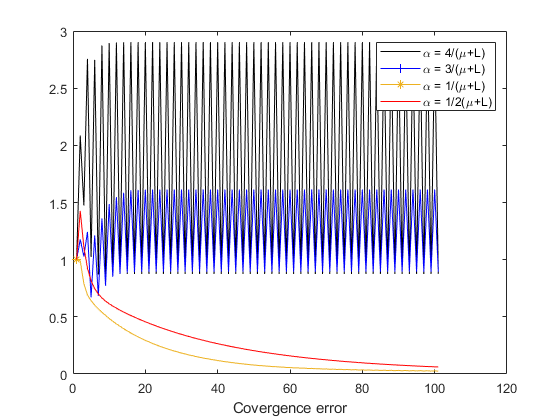
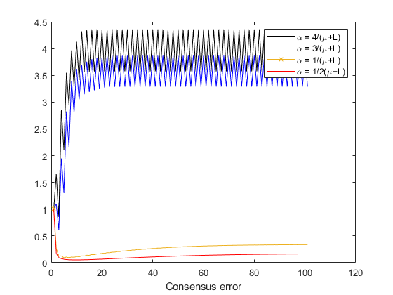
Figure 1. The left figure corresponds to the value $R_{1}(t)$ and the right figure corresponds to the value $R_{2}(t)$.

From Figure 1, we observe that the black and blue lines in the plot represent cases where the conditions in Theorems 2.2 and 2.3 are violated, while the other lines satisfy the conditions. Although both the black and blue lines do not converge to zero, they still appear to be bounded and oscillate within a certain range. On the other hand, for the other lines, both $R_{1}(t)$ and $R_{2}(t)$ properly converge to a small neighborhood of zero.

Next, we consider the decreasing stepsize $\alpha(t)=0.5/(t+w)^{p}$ with $w$ satisfying $w^{p}=L+\mu$ for $p\in\{0.25,0.5,0.75,1\}$. The graphs of $R_{1}(t)$ and $R_{2}(t)$ are presented in Figure 2. The numerical result shows that the values of $R_{1}(t)$ and $R_{2}(t)$ converge to zero as expected in Theorem 2.4 and Theorem 2.5.

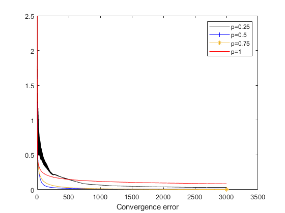
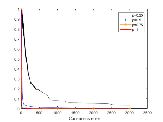
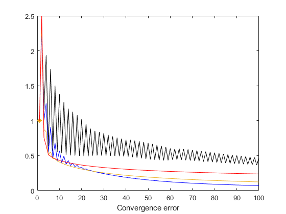
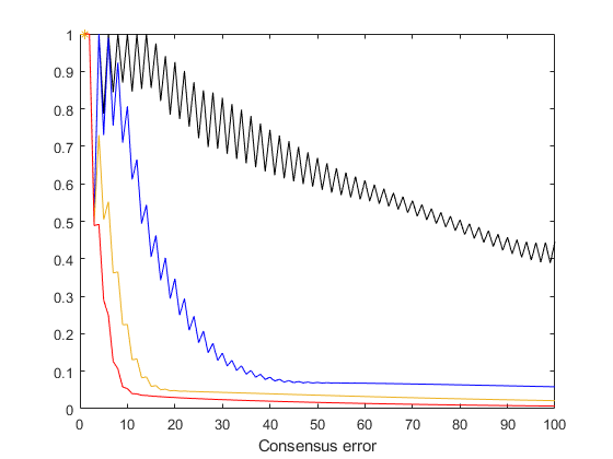
Figure 2. The values for $R_{1}(t)$ are listed in the first column and those for $R_{2}(t)$ are listed in the second columns. Each figure in the second row displays the first 100 iterations for each of the corresponding figures in the first row.

9.2. The example in Section 8

Here we provide a numerical test for the example considered in Section 8. Namely, we test the convergence property of the algorithm (8.3). To verify the result of Theorem 8.1, we consider the sequence $(x_{1}(t),x_{2}(t))$ of (8.3) and the following measure

$$R(t)=(x_{1}(t)-1)^{2}+\Big{(}x_{2}(t)-\frac{1}{1-18\alpha}\Big{)}^{2}\quad\textrm{for}~{}t\geq 0.$$ (9.1)

We test with the stepsizes $\{1/200,1/100,1/46,1/43\}$ and the initial values given as

$$(x_{1}(0),x_{2}(0))\in\{(5,10),(100,5)\}.$$ (9.2)

The graph of the normalized measure $R(t)/R(0)$ is provided in Figure 3. The result shows that the algorithm (8.3) converges to the value $(1,1/(1-18\alpha))$ for the stepsizes $\{1/200,1/100,1/46\}$ as expected by Theorem 8.1. Meanwhile, the algorithm (8.3) diverges for the stepsize $\alpha=1/43$ which is not supported in the interval $(0,1/45)$ guaranteed by Theorem 8.1. These results verify the sharpness of the result of Theorem 8.1.

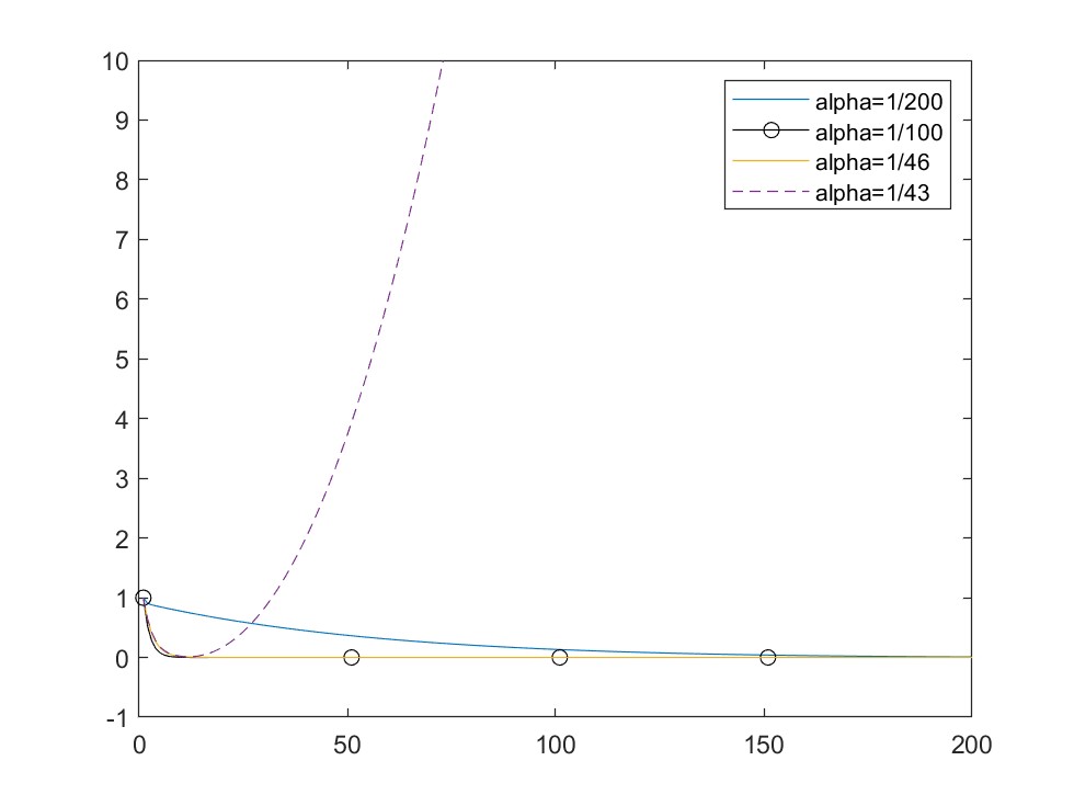
Figure 3. The left and right graphs represent the value $R(t)/R(0)$ for the initial values $(x_{1}(0),x_{2}(0))=(5,10)$ and $(100,5)$ respectively.

Conclusion. In this paper, we established new convergence estimates for the decentrlized projected gradient method. The result guarantees that the algorithm with stepsize $\alpha(t)\equiv\alpha>0$ converges to an $O(\sqrt{\alpha})$-neighborhood of the optimization, provided that $\alpha$ is less than a threshold. We also proved that this result can be improved to the convergence to an $O(\alpha)$-neighborhood for a specific example in dimension one. It remains an open question to extend the $O(\alpha)$ convergence result for general cases.

References

• [1] M. Akbari, B. Gharesifard, T. Linder, Distributed online convex optimization on time-varying directed graphs. IEEE Transactions on Control of Network Systems, 4(3), 417–428 (2015).
• [2] M. Assran, N. Loizou, N. Ballas, and M. Rabbat, Stochastic gradient push for distributed deep learning, in Proc. 36th Int. Conf. Mach. Learn., 2019, pp. 344–353.
• [3] S. Boyd, A. Ghosh, B. Prabhakar, and D. Shah, Randomized gossip algorithms, IEEE/ACM Transactions on Networking (TON), 14, no. SI, pp. 2508–2530, 2006.
• [4] L. Bottou, F. E. Curtis, and J. Nocedal, Optimization methods for large-scale machine learning, SIAM Review, vol. 60, no. 2, pp. 223–-311, 2018.
• [5] S. Bubeck, Convex optimization: Algorithms and complexity. Foundations and Trends R in Machine Learning, 8(3-4):231–357, 2015.
• [6] F. Bullo, J. Cortes, and S. Martinez, Distributed Control of Robotic Networks: A Mathematical Approach to Motion Coordination Algorithms, Princeton Series in Applied Mathematics (2009).
• [7] X. Cao, T. Basar (change s), Decentralized online convex optimization based on signs of relative states. (English summary) Automatica J. IFAC 129 (2021), Paper No. 109676, 13 pp.
• [8] Y. Cao, W. Yu, W. Ren, G. Chen, An overview of recent progress in the study of distributed multiagent coordination. IEEE Trans. Ind. Inform. 9(1), 427–-438 (2013)
• [9] W. Choi, J. Kim, On the convergence of decentralized gradient descent with diminishing stepsize, revisited, arXiv:2203.09079.
• [10] T. Doan, S. Maguluri, and J. Romberg, Finite-time analysis of distributed TD(0) with linear function approximation on multi-agent reinforcement learning, in Proc. Int. Conf. Mach. Learn., 2019, pp. 1626–1635.
• [11] I.-A. Chen et al., Fast distributed first-order methods, Master’s thesis, Massachusetts Institute of Technology, 2012.
• [12] P. A. Forero, A. Cano, and G. B. Giannakis, Consensus-based distributed support vector machines, Journal of Machine Learning Research, vol. 11, pp. 1663–-1707, 2010.
• [13] F. Facchinei and J.-S. Pang, Finite-Dimensional Variational Inequalities and Complementarity Problems. New York: Springer-Verlag, 2003
• [14] S. Hosseini, A. Chapman, M. Mesbahi, Online distributed convex optimization on dynamic networks. IEEE Trans. Automat. Control 61 (2016), no. 11, 3545–3550.
• [15] Y. Kajiyama, N. Hayashi, and S. Takai, Distributed subgradient method with edge-based event-triggered communication, IEEE Trans. Autom. Control, vol. 63, no. 7, pp. 2248–2255, Jul. 2018.
• [16] B. Jin, H. Li, W. Yan, M. Cao, Distributed model predictive control and optimization for linear systems with global constraints and time-varying communication, IEEE Trans. Automat. Control 66 (7) (2021) 3393–3400
• [17] C. Liu, H. Li, Y. Shi, and D. Xu, Distributed event-triggered gradient method for constrained convex optimization, IEEE Trans. Autom. Control, vol. 65, no. 2, pp. 778–785, Feb. 2020.
• [18] S. Liu, Z. Qiu, L. Xie, Convergence rate analysis of distributed optimization with projected subgradient algorithm. Automatica J. IFAC 83 (2017), 162–169.
• [19] A. Koloskova, N. Loizou, S. Boreiri, M. Jaggi, and S. Sebastian, A unified theory of decentralized SGD with changing topology and local updates. In International Conference on Machine Learning, 2020.
• [20] A. Nedić and A. Ozdaglar, Distributed subgradient methods for multi-agent optimization, IEEE Trans. Autom. Control 54 (2009), pp. 48–61.
• [21] A. Nedić and A. Olshevsky, Distributed optimization over time-varying directed graphs, IEEE Trans. Autom. Control 60 (2015), pp. 601–615.
• [22] A. Nedić, A. Olshevsky, Stochastic gradient-push for strongly convex functions on time-varying directed graphs. IEEE Trans. Automat. Control 61 (2016), no. 12, 3936–3947.
• [23] S. Pu and A. Nedić, Distributed stochastic gradient tracking methods, Math. Program, pp. 1–49, 2018
• [24] Q. Ling and Z. Tian, Decentralized sparse signal recovery for compressive sleeping wireless sensor networks, IEEE Trans. Signal Process., 58 (2010), pp. 3816–3827.
• [25] H. Raja and W. U. Bajwa, Cloud K-SVD: A collaborative dictionary learning algorithm for big, distributed data, IEEE Transactions on Signal Processing, vol. 64, no. 1, pp. 173–-188, Jan. 2016.
• [26] S. S. Ram, A. Nedić, and V. V. Veeravalli, Distributed Stochastic Subgradient Projection Algorithms for Convex Optimization, Journal of Optimization Theory and Applications, 147, no. 3, pp. 516–-545, 2010.
• [27] K. Yuan, Q. Ling, W. Yin, On the convergence of decentralized gradient descent. SIAM J. Optim., 26 (3), 1835–1854.