Entanglement quantification via nonlocality

Abstract

Nonlocality, manifested by the violation of Bell inequalities, indicates quantum entanglement in the underlying system. A natural question that arises is how much entanglement is required for a given nonlocal behavior. In this paper, we explore this question by quantifying entanglement using a family of generalized Clauser-Horne-Shimony-Holt-type Bell inequalities. We focus on two entanglement measures, entanglement of formation and one-way distillable entanglement, which are related to entanglement dilution and distillation, respectively. We also study the interplay among nonlocality, entanglement, and measurement incompatibility. The result reveals that the relationship between entanglement and measurement incompatibility is not simply a trade-off under a fixed nonlocal behavior. In addition, we consider two realistic scenarios non-maximally entangled states and Werner states and apply our entanglement quantification results. By optimizing the Bell inequality for entanglement estimation, we derive analytical results for the entanglement of formation.

I Introduction

In the early development of quantum mechanics, Einstein, Podolsky and Rosen noticed that the new physical theory leads to a “spooky action” between separate observables that is beyond any possible classical correlation [1]. Later, Bell formalizes such a quantum correlation via an experimentally feasible test that is now named after him [2]. In one of the simplest settings, the Clauser-Horne-Shimony-Holt (CHSH) Bell test [3], two distant experimentalists, Alice and Bob, each has a measurement device and share a pair of particles. While they may not know their devices and physical system a priori, they can each take random measurements and later evaluate the Bell expression,

$$S=\sum_{a,b,x,y}ab(-1)^{xy}p(a,b|x,y)=\sum_{x,y}(-1)^{xy}\mathbb{E}(ab|x,y),$$ (1)

where $x,y\in\{0,1\}$ represent their random choices of measurement settings and $a,b\in\{+1,-1\}$ denote their measurement results, as shown in Fig. 1. If Alice and Bob observe a value of $S>2$, then they cannot explain the observed correlation using any physical theory that follows local realism. This phenomenon is called Bell nonlocality. To demonstrate such a nonlocal behavior, the physical systems must exhibit a non-classical feature, wherein quantum theory, entanglement is such an ingredient [4]. The CHSH expression has a maximal value of $2\sqrt{2}$, which requires the maximally entangled state in a pair of qubits, $\ket{\Phi^{+}}=(\ket{00}+\ket{11})/\sqrt{2}$ [5]. We also term this state the Bell state.

Figure 1: A diagram of the CHSH Bell test. Two space-like separated users, Alice and Bob, share an unknown quantum state and own untrusted devices. In each round of the CHSH Bell test, Alice applies the measurement determined by the random input $x\in\{0,1\}$ and outputs her measurement result, $a\in\{\pm 1\}$. The measurement process is similar on Bob’s side, with input $y$ and output $b$. As the round of tests accumulated, the CHSH Bell value $S$ in Eq. (1) can be evaluated.

Entanglement characterizes a joint physical state among multiple parties that cannot be generated through local operations and classical communication (LOCC) [6, 7]. Beyond its role in understanding quantum foundations, entanglement is a useful resource in a variety of quantum information processing tasks, including quantum communication [8], quantum computation [9], and quantum metrology [10]. With a resource-theoretic perspective, a large class of information processing operations can be interpreted as entanglement conversion processes under LOCC, wherein one may quantify the participation of entanglement using appropriate measures [11, 12, 13, 14]. Therefore, the fundamental question is to detect and quantify entanglement in a system. While state tomography fully reconstructs the information of a quantum state and hence the entanglement properties [15, 16, 17], as detection loss and environmental noise are inevitable in practice, the tomography results may suffer from a precision problem. Notably, the measurement devices may not even be trusted in extreme adversarial scenarios.

Fortunately, quantum nonlocality provides a way to bypass the problem. Note that in the Bell test, one does not need to characterize the quantum devices a priori, and thus, the indication of entanglement from Bell nonlocality is a device-independent conclusion [18, 19]. This observation leads to the question of what the minimum amount of entanglement is necessary for a given nonlocal behavior. In other words, Bell tests can serve as a device-independent entanglement quantification tool. In the literature, there are already endeavors into the question [20, 21, 22]. The quantitative results provide us with tools for devising novel quantum information processing tasks. A notable investigation is the analysis of device-independent quantum key distribution [23, 18, 19]. With the link among nonlocality, entanglement, and secure communication, we can quantify the key privacy solely from Bell nonlocality [24, 25, 26].

Despite the physical intuition for entanglement quantification via Bell nonlocality, the quantitative relation between entanglement and nonlocality can be subtle [27]. Above all, while the notion of Bell nonlocality arises from the observation of correlations, entanglement is defined by the opposite of a restricted state preparation process. In fact, the Bell nonlocality is a stronger notion than entanglement. Though a nonlocal behavior necessarily requires the presence of entanglement, not all entangled states can unveil a nonlocal correlation [28]. The conceptual difference even leads to some counter-intuitive results, where a series of works aimed at characterizing their exact relation, such as the discussions on the Peres conjecture — whether Bell nonlocality is equivalent to distillability of entanglement [29, 30].

In addition, there are different entanglement measures that enjoy distinct operational meanings. As entanglement is not a reversible theory, these measures are generally not identical with each other [31]. An interesting yet vague question is whether different entanglement measures from nonlocal behavior can be the same.

In this work, we systematically study entanglement quantification via a family of generalized CHSH-type Bell inequalities. We treat the measurement devices as black boxes. Different implementations can lead to the same observed nonlocal behavior. As depicted in Fig. 2, a nonlocal behavior necessarily needs both entanglement and incompatible local measurements. In other words, a system with separable states or compatible local measurements definitely fails to observe nonlocality. One may expect a trade-off relationship between state entanglement and measurement incompatibility for a given nonlocal behavior. Hence, we explore the interplay among entanglement, nonlocality, and measurement incompatibility with different entanglement measures.

Figure 2: The interplay among nonlocality, entanglement, and measurement incompatibility. A nonlocal behavior necessarily indicates both entanglement and incompatible local measurements. A system with separable states or compatible local measurements fails in exhibiting nonlocality. Intuitively, under a given nonlocal behavior, one may expect a trade-off relationship between entanglement and measurement incompatibility. In this work, we start from the entanglement quantification via nonlocality, from which we realize that the relation between entanglement and measurement incompatibility is subtler than a simple trade-off. We study the interplay among nonlocality, entanglement, and measurement incompatibility in detail.

The rest of the paper is organized as follows. In Sec. II, we review the necessary concepts in nonlocality and entanglement theories. In Sec. III, we present the general framework for estimating entanglement in the underlying system using the set of generalized CHSH-type Bell inequalities. Then, we consider two special entanglement measures, the entanglement of formation and the one-way distillable entanglement. In Sec. IV, we utilize the entanglement quantification results and investigate the interplay among nonlocality, entanglement, and measurement incompatibility. From a practical perspective, in Sec. V, we also simulate statistics that arise from pure entangled states and Werner states and examine the performance of our results.

II Preliminary

II.1 General CHSH-type Bell tests

In this work, we consider the family of generalized CHSH-type Bell tests. Under quantum mechanics, the Bell expression is given by [27]

$$\begin{split}S&=\Tr[\rho_{AB}\left(\alpha\hat{A_{0}}\otimes\hat{B_{0}}+\alpha\hat{A}_{0}\otimes\hat{B}_{1}+\hat{A}_{1}\otimes\hat{B}_{0}-\hat{A}_{1}\otimes\hat{B}_{1}\right)]\\ &=\Tr(\rho_{AB}\hat{S}_{\alpha}),\end{split}$$ (2)

where $\rho_{AB}$ is the underlying bipartite quantum state, $\hat{A}_{x}$ and $\hat{B}_{y}$ are the observables measured by Alice and Bob, according to their measurement choices, $x,y\in\{0,1\}$, respectively. The family of Bell expressions is parameterized by $\alpha\geq 1$, which tilts the contributions of $\hat{A}_{0}\otimes(\hat{B}_{0}+\hat{B}_{1})$ and $\hat{A}_{1}\otimes(\hat{B}_{0}-\hat{B}_{1})$ to the Bell value. When $\alpha=1$, Eq. (2) degenerates to the original CHSH expression defined by Eq. (1) [3]. For simplicity, we call the expression under the fixed parameter of $\alpha$ as $\alpha$-CHSH expression and $\hat{S}_{\alpha}$ the $\alpha$-CHSH operator. If the underlying quantum state is separable or the local measurement observables are compatible, the $\alpha$-CHSH expression is upper bounded by $S(\alpha)\leq 2\alpha$, which commits a local hidden variable model to reproduce the correlation. Observation of a larger value, termed Bell inequality violation, necessarily implies the existence of entanglement and measurement incompatibility between the local measurement observables. In quantum theory, the largest value of $\alpha$-CHSH expression is $2\sqrt{\alpha^{2}+1}$.

In the study of Bell nonlocality, we do not put prior trust in the underlying physical systems. In particular, we do not assume a bounded system dimension. Nevertheless, the simplicity of CHSH-type Bell expressions allows us to apply Jordan’s lemma to effectively reduce the system to a mixture of qubit pairs [19]. We shall explain how to apply this result when we come to the part of main results.

II.2 Entanglement measures

As our discussion is effectively restricted to a pair of qubits, we shall focus on a few entanglement measures that enjoy a closed form in such a case. We consider $\rho_{AB}$ as a pair of qubits here. The first measure we consider is the entanglement of formation, $E_{\mathrm{F}}(\rho_{AB})$ [14]. Operationally, this measure provides a computable bound on the entanglement cost, which quantifies the optimal state conversion rate of diluting maximally entangled states into the desired states of $\rho_{AB}$ under LOCC [14]. In the case of two-qubit states, we can calculate the entanglement of formation with the following expression,

$$E_{\mathrm{F}}(\rho_{AB})=h\left(\frac{1+\sqrt{1-C^{2}(\rho_{AB})}}{2}\right),$$ (3)

where $h(p)=-p\log p-(1-p)\log(1-p)$ is the binary entropy function, and $C(\rho_{AB})$ is the concurrence of $\rho_{AB}$, a useful entanglement monotone [32, 33]. Given a general two-qubit quantum state, $\rho_{AB}$, its concurrence is analytically given by

$$C(\rho_{AB})=\max\{0,\lambda_{1}-\lambda_{2}-\lambda_{3}-\lambda_{4}\},$$ (4)

where values $\lambda_{i}$ are the decreasingly ordered square roots of the eigenvalues of the matrix

$$X(\rho_{AB})=\sqrt{\rho_{AB}}(\sigma_{y}\otimes\sigma_{y})\rho_{AB}^{*}(\sigma_{y}\otimes\sigma_{y})\sqrt{\rho_{AB}}.$$ (5)

Here, the density matrix of $\rho_{AB}$ is written on the computational basis of $\{\ket{00},\ket{01},\ket{10},\ket{11}\}$, where $\ket{0}$ and $\ket{1}$ are the eigenstates of $\sigma_{z}$, and $\rho_{AB}^{*}$ is the complex conjugate of $\rho_{AB}$.

As opposed to the entanglement dilution process, the entanglement distillation process defines another entanglement measure, the distillable entanglement [14]. In this process, given sufficiently many copies of a given state, $\rho_{AB}$, the distillable entanglement is the maximal state conversion rate of distilling maximally entangled states under LOCC. While the calculation of this measure for a general state remains an open question, a well-studied lower bound is the one-way distillable entanglement, where classical communication is restricted to a one-way procedure between the two users. This measure can be calculated by the negative conditional entropy,

$$E_{D}^{\rightarrow}(\rho_{AB})=-H(A|B)_{\rho},$$ (6)

where $H(A|B)_{\rho}=H(\rho_{AB})-H(\rho_{B})$. When the underlying state is clear from the context, we shall omit the subscript for simplicity.

We remark that the above results of entanglement measures are defined via dilution and distillation processes with infinitely many independent and identical (i.i.d.) copies of the quantum state under study or, in the i.i.d. asymptotic limit. In this work, we shall focus on the entanglement quantification via Bell nonlocality in this limit. That is, we treat both the amount of entanglement and the Bell value as expected values.

III Device-independent entanglement quantification

III.1 Entanglement quantification via optimization

In this section, we formulate the problem of entanglement quantification via Bell nonlocality. Using the nomenclature in quantum cryptography, we also term it device-independent entanglement quantification. After specifying a particular entanglement measure, $E$, we ask the minimal amount of entanglement in the initial quantum system that supports the observed Bell expression value,

$$\begin{split}E_{\rm est}&=\min_{\rho_{AB},\hat{A}_{0},\hat{A}_{1},\hat{B}_{0},\hat{B}_{1}}E(\rho_{AB}),\\ \text{s.t.}\quad S&=\Tr\left(\rho_{AB}\hat{S}_{\alpha}\right),\\ \rho_{AB}&\geq 0,\\ \Tr(\rho_{AB})&=1.\end{split}$$ (7)

Here, we denote the estimated entanglement measure of $E$ from Bell nonlocality as $E_{\rm est}$. As clarified above, $\hat{S}_{\alpha}$ is the $\alpha$-CHSH operator, an operator function of the measurement observables.

The optimization problem is difficult to solve directly. First, it involves multiple variables, including the underlying state and the measurement observables. Second, we do not have empirical knowledge of the system dimension. In Eq. (7), the dimension of $\rho_{AB}$ is unknown. Thus we cannot solve this optimization problem. To get around these issues, we degenerate its solution into several steps, as shown in Fig. 3.

Figure 3: Steps for estimating entanglement via CHSH-type Bell inequalities. Step 1: The original entanglement estimation problem is formulated as Eq. (7). The only constraint is the observed Bell value, $S$. Step 2: Using a duality argument, we consider the optimization problem in Eq. (8), which can be interpreted as maximizing the Bell value for a given quantum state, $\rho_{AB}$. The arguments in the optimal solution are regarded as the “optimal measurements” that lead to the maximal Bell value for the state. Step 3: By applying Jordan’s lemma, we can view the measurement process as resulting from a convex combination of pairs of qubits. Step 4: We can further restrict the qubit pairs to Bell-diagonal states in solving the optimization problem. We show that in the CHSH Bell test, any two-qubit state can be transformed to a Bell-diagonal state through LOCC without changing the $\alpha$-CHSH Bell value.

In the first step, we use duality arguments and transform Eq. (7). Note that the objective function in Eq. (7), $E_{\rm est}:=f(S)$, is continuous and monotonously increasing in its argument $S$, hence having a well-defined inverse function. Consider the following problem,

$$\begin{split}S^{*}&=\max_{\rho_{AB},\hat{A}_{0},\hat{A}_{1},\hat{B}_{0},\hat{B}_{1}}\Tr\left(\rho_{AB}\hat{S}_{\alpha}\right),\\ \text{s.t.}\quad E(\rho_{AB})&=E_{\rm est},\\ \rho_{AB}&\geq 0,\\ \Tr(\rho_{AB})&=1,\end{split}$$ (8)

where the objective function in Eq. (8) comes from the inverse function of the original optimization problem, $S^{*}:=f^{-1}(E_{\rm est})$. In solving Eq. (8), as the objective function is bilinear in $\rho_{AB}$ and Bell operator $\hat{S}_{\alpha}$, the optimization equals the maximization over the two arguments individually, $S^{*}=\max_{\rho_{AB}}\max_{\hat{A}_{0},\hat{A}_{1},\hat{B}_{0},\hat{B}_{1}}\Tr\left(\rho_{AB}\hat{S}_{\alpha}\right)$. For the inner optimization, denote $S^{*}(\rho_{AB})=\max_{\hat{A}_{0},\hat{A}_{1},\hat{B}_{0},\hat{B}_{1}}\Tr\left(\rho_{AB}\hat{S}_{\alpha}\right)$, which can be seen as the maximal $\alpha$-CHSH Bell value that can be obtained with $\rho_{AB}$. Then, we may equivalently solve Eq. (7) with the following optimization,

$$\begin{split}E_{\rm est}&=\min_{\rho_{AB}}E(\rho_{AB}),\\ \text{s.t.}\quad S^{*}(\rho_{AB})&=S,\\ \rho_{AB}&\geq 0,\\ \Tr(\rho_{AB})&=1.\end{split}$$ (9)

For simplicity, we call the measurements that yield the maximal $\alpha$-CHSH Bell value for $\rho_{AB}$ the “optimal measurements”.

Definition 1.

The optimal measurements of state $\rho_{AB}$ are the observables that maximize the $\alpha$-CHSH expression in Eq. (2) for $\rho_{AB}$, i.e., $\operatorname{argmax}_{\hat{A}_{0},\hat{A}_{1},\hat{B}_{0},\hat{B}_{1}}\Tr\left(\rho_{AB}\hat{S}_{\alpha}\right)$.

To bypass the dimension problem, we utilize Jordan’s lemma. We leave the detailed analysis in Appendix A.1. Here, we briefly state the indication of Jordan’s lemma in our work. In the CHSH-type Bell test, we can effectively view the measurement process as first performing local operations to transform the underlying quantum state into an ensemble of qubit pairs, $\{p^{\mu},\rho_{AB}^{\mu}\}$, with $p^{\mu}$ a probability distribution, and then measuring each pair of qubits with associate qubit observables. The measurement on each pair of qubits corresponds to a Bell value, $S^{\mu}$, and the observed Bell value is the average of these values, $S=\sum_{\mu}p^{\mu}S^{\mu}$. Guaranteed by the convexity property of an entanglement measurement, we can lower-bound the amount of entanglement in the initial system by studying the average amount of entanglement in the ensemble of qubit-pairs, $\sum_{\mu}p^{\mu}E(\rho_{AB}^{\mu})$. In this way, we can essentially focus on quantifying entanglement in a pair of qubits.

By further utilizing the non-increasing property under LOCC of an entanglement measure and choosing proper local computational bases, we may further restrict the pair of qubits to a diagonal state on the Bell-state basis,

$$\rho_{\lambda}=\lambda_{1}\outerproduct{\Phi^{+}}{\Phi^{+}}+\lambda_{2}\outerproduct{\Phi^{-}}{\Phi^{-}}+\lambda_{3}\outerproduct{\Psi^{+}}{\Psi^{+}}+\lambda_{4}\outerproduct{\Psi^{-}}{\Psi^{-}},$$ (10)

with $\ket{\Phi^{\pm}}=(\ket{00}\pm\ket{11})/\sqrt{2},\ket{\Psi^{\pm}}=(\ket{01}\pm\ket{10})/\sqrt{2}$. We term such a state a Bell-diagonal state with respect to the computational basis. Without loss of generality, we assume $\lambda_{1}\geq\lambda_{2}\geq\lambda_{3}\geq\lambda_{4}$, since we can relabel the eigenvalues corresponding to the Bell-basis states with local unitary operations.

Lemma 1.

In a CHSH Bell test, under a fixed computational basis, a two-qubit state, $\rho_{AB}$, can be transformed into a Bell-diagonal state, $\rho_{\lambda}$, through LOCC, with the $\alpha$-CHSH Bell value unchanged.

The lemma indicates that an observed Bell value can always be interpreted as arising from a Bell-diagonal state. Furthermore, the operations in the lemma are restricted to LOCC and state mixing. Since these operations do not increase entanglement, we can hence restrict our analysis of lower-bounding entanglement to the set of Bell-diagonal states. The LOCC transformation in this result was first constructed in Ref. [34] (see Lemma 3 therein). Here, we verify the unchanged $\alpha$-CHSH Bell value through the LOCC transformation. We present proof of the lemma in Appendix A.2.

With the above simplifications, we have the following lemma in solving the problem in Eq. (9).

Lemma 2.

The maximal value of the $\alpha$-CHSH expression in Eq. (2) for a Bell-diagonal state shown in Eq. (10), $\rho_{\lambda}$, is given by

$$S=2\sqrt{\alpha^{2}(\lambda_{1}+\lambda_{2}-\lambda_{3}-\lambda_{4})^{2}+(\lambda_{1}-\lambda_{2}+\lambda_{3}-\lambda_{4})^{2}},$$ (11)

where $\lambda_{i}$ is the $i$-th largest eigenvalue of $\rho_{\lambda}$.

We give the proof of Lemma 2 in Appendix A.2. For two projective measurements, their incompatibility is defined as the largest inner product of their eigenvectors. For qubit observables, this definition is equivalent to the commutator. In proving Lemma 2, a notable issue is that the optimal measurements may not be the most incompatible measurements. Up to a minus sign before the observables, the optimal measurements of the Bell-diagonal state in Eq. (10) are as follows,

$$\begin{split}\hat{A}_{0}&=\sigma_{z},\\ \hat{A}_{1}&=\sigma_{x},\\ \hat{B}_{0}&=\cos\theta\sigma_{z}+\sin\theta\sigma_{x},\\ \hat{B}_{1}&=\cos\theta\sigma_{z}-\sin\theta\sigma_{x},\end{split}$$ (12)

where $\theta$ fully determines the amount of imcompatibility of the local observables, with $\tan\theta=(\lambda_{1}-\lambda_{2}+\lambda_{3}-\lambda_{4})/[\alpha(\lambda_{1}+\lambda_{2}-\lambda_{3}-\lambda_{4})]$ determined by the Bell-diagonal state and parameter $\alpha$. While the observables on Alice’s side are maximally incompatible with each other, the commutator of the observables on Bob’s side is given by $[\hat{B}_{0},\hat{B}_{1}]=\sin 2\theta[\sigma_{x},\sigma_{z}]$. For example, when the considered state is the maximally entangled state with $\lambda_{1}=1,\lambda_{2}=\lambda_{3}=\lambda_{4}=0$ and $\alpha=1$, which corresponds to the original CHSH expression, the optimal measurements coincide with the most incompatible measurements. For more cases where $\sin 2\theta$ is strictly smaller than $1$, $\hat{B}_{0}$ and $\hat{B}_{1}$ are not maximally incompatible.

Observation 1.

The observables that yield the largest $\alpha$-CHSH Bell value for a quantum state are not the most incompatible ones in general.

Notwithstanding, a subtle issue is that we do not have access to the underlying probability distribution in the qubit-pair ensemble, $p^{\mu}$, or the underlying Bell value for each pair of qubits. As we only know the average Bell value over the ensemble, we need to be careful of convexity issues. Suppose the solution to Eq. (7) with the restriction of a pair of qubits takes the form $E_{\rm est}=E_{\rm est}(S)$. When extending the result to possibly an ensemble of qubit pairs, if $E_{\rm est}(S)$ is not convex in $S$, then

$$E_{\rm est}\left(\sum_{\mu}p^{\mu}S^{\mu}\right)\leq\sum_{\mu}p^{\mu}E_{\rm est}\left(S^{\mu}\right)\leq\sum_{\mu}p^{\mu}E\left(\rho_{AB}^{\mu}\right)\leq E(\rho_{AB}),$$ (13)

which holds for any probability distribution $p^{\mu}$. Hence, we can directly lower-bound the amount of entanglement in the underlying state by $E_{\rm est}(S)$, where $S=\sum_{\mu}p^{\mu}S^{\mu}$ represents the observed Bell value. Yet if the function $E_{\rm est}(S)$ is concave, then the first inequality above no longer holds valid. Consequently, we need to take a convex closure of the function $E_{\rm est}$ to estimate the amount of entanglement from a quantum state with an unknown dimension.

Following the above discussions, we study the entanglement measures of entanglement of formation and one-way distillable entanglement, which are essentially given by concurrence and conditional entropy of entanglement, respectively.

III.2 Concurrence and entanglement of formation

In this subsection, we take concurrence $C(\cdot)$ as the objective entanglement measure in Eq. (7). For this measure, we have an analytical estimation result.

Theorem 1.

Suppose the underlying quantum state is a pair of qubits. For a given tilted CHSH expression in Eq. (2) parametrized by $\alpha$, if the Bell expression value is $S$, then the amount of concurrence in the underlying state can be lower-bounded,

$$C(\rho_{AB})\geq\sqrt{\frac{S^{2}}{4}-\alpha^{2}}.$$ (14)

The equality can be saturated when measuring a Bell-diagonal state in Eq. (10) with eigenvalues

$$\begin{gathered}\lambda_{1}=\frac{1}{2}+\frac{1}{2}\sqrt{\frac{S^{2}}{4}-\alpha^{2}},\\ \lambda_{2}=\frac{1}{2}-\frac{1}{2}\sqrt{\frac{S^{2}}{4}-\alpha^{2}},\\ \lambda_{3}=\lambda_{4}=0,\end{gathered}$$ (15)

using measurements in Eq. (12) with $\theta=\arctan(\frac{1}{\alpha}\sqrt{\frac{S^{2}}{4}-\alpha^{2}})$.

We leave the detailed derivation in Appendix B.

Observation 2.

Given a $\alpha$-CHSH Bell value, the measurements that require the minimum entanglement are not the most incompatible measurements in general.

As the entanglement of formation can be expressed by concurrence in a closed form for a pair of qubits, this entanglement measure is directly lower-bounded,

$$E_{\rm F}(\rho_{AB})\geq h\left(\frac{1}{2}+\frac{1}{2}\sqrt{1+\alpha^{2}-\frac{S^{2}}{4}}\right).$$ (16)

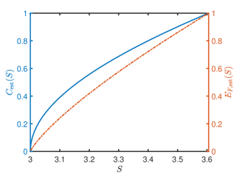
Figure 4: Diagram of concurrence and entanglement formation estimation results when the CHSH-type expression in Eq. (2) takes $\alpha=1.5$ and input states are two-qubit states. We plot the estimated values of concurrence and entanglement of formation with the blue solid line and the red dashed line, respectively. The estimations are both concave in $S\in(3,2\sqrt{3.25}]$ and range from $0$ to $1$.

In Fig. 4, we depict the entanglement estimation result when $\alpha=1.5$ for a pair of qubits input. As can be seen from the curves, the functions that give the estimated amount of entanglement are concave in the Bell value. As we discussed above, we should take a convex closure for the measures when extending the results to general states with an unknown dimension. Therefore, the final estimation is given by

$$C(\rho_{AB}),E_{\rm F}(\rho_{AB})\geq\frac{S-2\alpha}{2\sqrt{1+\alpha^{2}}-2\alpha}.$$ (17)

III.3 Negative conditional entropy and one-way distillable entanglement

In this subsection, we estimate the one-way distillable entanglement, $E_{D}^{\rightarrow}(\rho_{AB})$, depicted by the negative conditional entropy, $-H(A|B)$, via Bell nonlocality. For the set of Bell-diagonal states on the qubit-pair systems, since the reduced density matrix of a subsystem is a maximally mixed state, $H(B)=1$, the conditional von Neumann entropy of the state is reduced to $H(A|B)=H(AB)-H(B)=H(AB)-1$. Using the notation in Eq. (10), the term of joint von Neumann entropy can be expressed by

$$H(AB)=H(\vec{\lambda})=-\sum_{i=1}^{4}\lambda_{i}\log\lambda_{i}.$$ (18)

Thus, the lower bound of one-way distillable entanglement for a pair of qubits becomes the following optimization problem,

$$\begin{split}E_{D\rm,est}^{\rightarrow}&=\underset{\lambda_{i},i=1,2,3,4}{\text{min}}1+\sum_{i=1}^{4}\lambda_{i}\log\lambda_{i},\\ \text{s.t.}\quad S&=2\sqrt{\alpha^{2}(\lambda_{1}+\lambda_{2}-\lambda_{3}-\lambda_{4})^{2}+(\lambda_{1}-\lambda_{2}+\lambda_{3}-\lambda_{4})^{2}},\\ \lambda_{1}&\geq\lambda_{2}\geq\lambda_{3}\geq\lambda_{4},\\ 1&=\sum_{i=1}^{4}\lambda_{i},\lambda_{i}\geq 0\;,i=1,2,3,4.\end{split}$$ (19)

As this is a convex optimization problem, we can solve it efficiently via off-the-shelf numerical toolboxes. We present numerical results for some values of $\alpha$ in Fig. 5. Given any $\alpha>1$, the estimation value $E_{D\rm,est}^{\rightarrow}(S)$ is a convex function on $S\in(2\alpha,2\sqrt{1+\alpha^{2}}]$. Following Eq. (13), the solution can be directly lifted as the lower bound on one-way distillable entanglement for a general state.

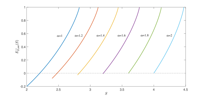
Figure 5: Diagram of one-way distillable entanglement estimation results. The estimation is depicted by CHSH-type Bell expressions with several discretely increasing $\alpha$. For each value of $\alpha$, the estimation result, $E_{D\rm,est}^{\rightarrow}(S)$, depicted over the valid interval $S\in(2\alpha,2\sqrt{1+\alpha^{2}}]$ is convex. When $\alpha$ increases, $E_{D\rm,est}^{\rightarrow}(S)$ at $S=2\alpha$ for each $\alpha$ increases and converges to $0$. Since $E_{D,\rm est}^{\rightarrow}(S)$ is convex in $S$, the estimation results hold valid without assuming the system dimension.

IV Interplay among entanglement, measurement incompatibility, and nonlocality

Besides entanglement, another key ingredient behind nonlocality is measurement incompatibility. Both entanglement and measurement compatibility can be regarded as quantum resources to unveil non-classical physical phenomena. Hence a natural intuition is that for a given Bell value, there is a trade-off relation between entanglement and measurement incompatibility, where more incompatible measurement may compensate an underlying system with less entanglement and vice versa. However, as we have discussed for the notion of optimal measurements, the observables that yield the largest Bell value for a quantum state may not correspond to the maximally incompatible ones. Particularly, as shown in Theorem 1, for the case of the least amount of entanglement for a nonlocal behavior, the observables are generally not maximally incompatible. In this section, we make a detailed investigation into the relation between entanglement and measurement incompatibility under a given Bell nonlocal behavior.

To simplify the discussion, we restrict our analysis with the following assumptions: (1) the underlying system is a pair of qubits, and (2) the measurement operators are qubit observables. Note that in the fully device-independent scenario without any a priori assumption, the measurement result is a mixture of basic scenarios in this form, which can be shown by Jordan’s lemma. In a sense, the situation we look at represents a typical setting for the question. To characterize a nonlocal behavior, we use the value of a particular $\alpha$-CHSH Bell expression.

We quantify the least amount of entanglement that is necessary for a given Bell value,

$$\begin{split}E_{\mathrm{est}}&=\min_{\rho_{AB}}E(\rho_{AB}),\\ \text{s.t.}\quad\Tr\left(\rho_{AB}\hat{S}_{\alpha}\right)&=S,\\ \hat{A}_{0}&=\sigma_{z},\\ \hat{A}_{1}&=\sigma_{x},\\ \hat{B}_{0}&=\cos\theta\sigma_{z}+\sin\theta\sigma_{x},\\ \hat{B}_{1}&=\cos\theta\sigma_{z}-\sin\theta\sigma_{x},\\ \rho_{AB}&\geq 0,\\ \rho_{AB}&\in\mathcal{D}(\mathcal{H}_{2}\otimes\mathcal{H}_{2}),\\ \Tr(\rho_{AB})&=1.\end{split}$$ (20)

where $E$ represents a chosen entanglement measure. We still denote the solution to the optimization as $E_{\mathrm{est}}$, while it now represents the least amount of entanglement that is necessary for the nonlocal behavior under the given measurement incompatibility. In this optimization, we assume that the measurement incompatibility is parameterized by one parameter, $\theta$. On Alice’s side, the two local observables are fixed to be maximally incompatible with each other. On Bob’s side, when $\theta=0$ and $\pi/2$, the two local observables commute. When $\theta=\pi/4$, the local observables enjoy the maximal incompatibility, which is the other extreme. In the following discussions, we restrict the parameter to be $\theta\in[0,\pi/4]$, as other cases can be obtained via symmetry. As there are two nonlocal parties in the Bell nonlocality setting, one may investigate measurement incompatibility with possibly other scenarios. We choose this scenario since that, for any given quantum state, one may encounter its optimal measurements by varying $\theta$. In fact, if the measurements in Eq. (20) become optimal for $\rho_{AB}$, the solution to Eq. (20) coincides with the solution to Eq. (9) under the system dimension constraint. In this way, the solution to Eq. (20) should reach the tight lower bound of device-independent entanglement estimation in a proper measurement setting.

IV.1 Original CHSH ($\alpha=1$)

To observe the interplay among entanglement, measurement incompatibility, and nonlocality, we numerically solve the optimization problem in Eq. (20) by taking concurrence and one-way distillable entanglement as an entanglement measure and varying $\theta\in[0,\pi/4]$ and $S$ discretely from the $\alpha$-CHSH Bell values.

In Fig. 6, we choose the original CHSH Bell expression and present the numerical results when taking the concurrence as the entanglement measure. For a nonlocal behavior, where $S\in(2,2\sqrt{2}]$, we denote $\theta=\theta_{C}^{*}$ when the estimated concurrence reaches its minimum, $C_{\rm est}(S,\theta)=\sqrt{S^{2}/4-1}$. As we have derived in Theorem 1, $\theta_{C}^{*}=\arctan\sqrt{S^{2}/4-1}$. When the amount of measurement incompatibility between the local observables is smaller than that of this point, which corresponds to $\theta<\theta_{C}^{*}$, there is a trade-off relation between concurrence and measurement incompatibility, where less entanglement is required for the given Bell value as the amount of measurement incompatibility increases. However, when $\theta>\theta_{C}^{*}$, as the underlying state enjoys more entanglement of concurrence, larger measurement incompatibility is also required for the observed Bell value. As $S$ increases from $2$ to $2\sqrt{2}$, the range of feasible values of $(\theta,C_{\mathrm{est}})$ shrinks as $S$ grows. When $S=2\sqrt{2}$, the underlying state is maximally entangled and the local measurement observables are the most incompatible ones, and the range of possible values of $(\theta,C_{\mathrm{est}})$ degenerates to the point of $(\pi/4,1)$. This result coincides with the self-testing finding [35], where the only feasible experimental setting for the maximum CHSH Bell value enjoys the above properties.

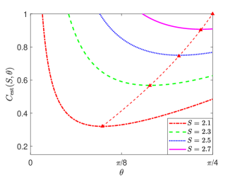
Figure 6: Illustration of the interplay among Bell nonlocality, measurement incompatibility, and concurrence. In this figure, we consider the original CHSH Bell expression and parameterize the measurement observables as in Eq. (12), where incompatibility is quantified through $\theta$. We focus on the interval of $\theta\in[0,\pi/4]$, and the results elsewhere can be obtained using symmetry. For a given value of $S$, when $\theta<\theta_{C}^{*}=\arctan\sqrt{S^{2}/4-1}$, there is a trade-off relation between entanglement and measurement incompatibility, where less entanglement of concurrence is required for the nonlocal behavior when the measurements become more incompatible and vice versa. Afterward, more entanglement is required for the given Bell value as $\theta$ increases. As $S$ increases, the range of possible values of $(\theta,C_{\mathrm{est}})$ shrinks and $\theta_{C}^{*}$ gets close to $\pi/4$.

In Fig. 7, we present the numerical results when taking the one-way distillable entanglement as the entanglement measure. Under a fixed Bell value, there is a strict trade-off relation between entanglement and measurement incompatibility. The more incompatible the measurement observables are, the less entanglement is necessary for the nonlocal behavior, and vice versa. In addition, the range for the trade-off shrinks with a larger Bell violation value. In the extreme of the largest Bell violation value, $S=2\sqrt{2}$, the setting should involve both the maximally entangled state and measurement observables that are maximally incompatible, in accordance with the self-testing result. One thing to note is that the estimated negative conditional entropy reaches its minimum exactly when $\theta=\pi/4$ for all $S\in(2,2\sqrt{2}]$, which holds no longer valid in $\alpha$-CHSH inequality when $\alpha>1$.

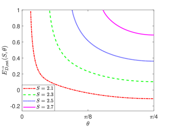
Figure 7: Illustration of the interplay among Bell nonlocality, measurement incompatibility, and one-way distillable entanglement. In this figure, we consider the original CHSH Bell expression and parameterize the measurement observables as in Eq. (12). As $S$ increases, the range of possible values of $(\theta,E_{D,{\rm est}}^{\rightarrow})$ shrinks. For a given Bell value, less entanglement is required when $\theta$ increases in the valid region.

IV.2 General CHSH-type ($\alpha>1$)

Besides the original CHSH Bell expression, we also study the relation among entanglement, measurement incompatibility, and nonlocality for general $\alpha$-CHSH expressions. Fixing parameter $\alpha>1$, for any Bell value $S\in(2\alpha,2\sqrt{1+\alpha^{2}}]$, denote the range of plausible values of parameter $\theta$ by $\theta_{\min}\leq\theta\leq\theta_{\max}$. In Fig. 8, we investigate the issue under parameter $\alpha=1.2$. For both the concurrence of entanglement and one-way distillable entanglement, when $\theta$ increases from $\theta_{\min}$ to $\theta_{\max}$, the corresponding amount of estimated entanglement first monotonically decreases from $1$, which corresponds to the maximally entangled state. In this region, there is a trade-off relation between entanglement and measurement incompatibility under the given Bell value. After reaching its minimum at $\theta=\theta^{*}_{E}$, a point that is related to the particular entanglement measure under study, more entanglement is required as the local measurement observables become more incompatible. One thing worth noting is that under the same $S$, the values of $\theta_{\min}$ and $\theta_{\max}$ are the same for both entanglement measures we now study. As $S$ grows, the supported range of incompatibility and entanglement shrinks, which converges to the single point of $\theta=\arctan(1/\alpha)$ and $E_{\rm est}=1$ when $S$ approaches its maximum $2\sqrt{1+\alpha^{2}}$. Namely, the maximum value of the $\alpha$-CHSH expression requires a pair of non-maximally incompatible measurements on one side. This result also coincides with the self-testing findings [27]. Another indication is that to yield a large $\alpha$-CHSH Bell value with $\alpha>1$, the measurement observables on one side cannot be too incompatible, where they lie outside the feasible region of the experimental settings.

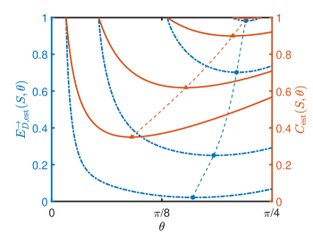
Figure 8: Illustration of the interplay among Bell nonlocality, measurement incompatibility, and entanglement. In this figure, we consider the $\alpha$-CHSH Bell expression with $\alpha=1.2$. The blue curves depict the results of one-way distillable entanglement, and the red curves depict the results of concurrence. For both entanglement measures, given a Bell value, the least required amount of entanglement first monotonically decreases as $\theta$ increases. After $\theta$ is larger than a threshold value that depends on the entanglement measure, $\theta_{E}^{*}$, more entanglement is required as the measurements become more incompatible. The ranges of possible values of $\theta\in[\theta_{\min},\theta_{\max}]$ are the same for the two entanglement measures. When $S<2.2\sqrt{2}$, $\theta_{\max}=\pi/4$. When $S\geq 2.2\sqrt{2}$, $\theta_{\max}$ is smaller than $\pi/4$. The supported range shrinks as $S$ increases. When $S$ reaches its maximum, $S=2\sqrt{1.2^{2}+1}$, the range degenerates to the point of $\theta=\arctan 1/1.2$. In this case, the underlying state can only be a maximally entangled state, corresponding to $E_{\rm est}=1$.

For concurrence, we can derive the critical points analytically. Given $\alpha$-CHSH Bell value $S$, when $\theta=\theta^{*}_{C}=\arctan(\frac{1}{\alpha}\sqrt{\frac{S^{2}}{4}-\alpha^{2}})$, the system requires the least amount of concurrence, $C_{\mathrm{est}}=\sqrt{\frac{S^{2}}{4}-\alpha^{2}}$, which can be derived from Theorem 1. When $\theta>\theta_{C}^{*}$, we find there is a region of $\theta$ where the least amount of concurrence behaves differently from that of one-way distillable entanglement. That is, though more concurrence is required in the underlying system as $\theta$ grows, the system may yield less distillable entanglement. In other words, the manifestation of entanglement properties through nonlocality highly depends on the particular entanglement measure under study.

The value of $\theta_{\max}$ and the value of corresponding $E_{\mathrm{est}}$ are related to the parameter, $\alpha$. A notable issue is that under particular value of $\alpha$ and Bell value $S$, $E_{\mathrm{est}}$ at $\theta=\theta_{\max}$ can reach $1$. We find that when $1<\alpha<\sqrt{2}+1$, for $S<\sqrt{2}(\alpha+1)$, $\theta_{\max}=\pi/4$ and the corresponding least amount of entanglement, $E_{\rm est}$ is strictly smaller than $1$. For a larger Bell value, $S\geq\sqrt{2}(\alpha+1)$, $\theta_{\max}$ may be smaller than $\pi/4$, and $E_{\rm est}$ at $\theta=\theta_{\max}$ always reaches $E_{\rm est}=1$. For Bell expressions with $\alpha\geq\sqrt{2}+1$, as long as the Bell inequality is violated, $S>2\alpha$, we have $E_{\rm est}=1$ at $\theta=\theta_{\max}$. In Fig. 9, we illustrate the interplay relation when $\alpha=\sqrt{2}+1$. From this example, we can see that there can be two experimental settings that give rise to the same Bell value, where the underlying systems enjoy the same amount of entanglement, yet the incompatibility between the local measurements can be significantly different.

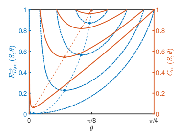
Figure 9: Illustration of the interplay among Bell nonlocality, measurement incompatibility, and entanglement. In this figure, $\alpha=\sqrt{2}+1$. The blue curves depict the results of one-way distillable entanglement, and the red curves depict the results of concurrence. The relation between entanglement and measurement incompatibility is similar to that in Fig. 8. Nevertheless, given any Bell value $S$ that is larger than $2\alpha$, which violates the $\alpha$-CHSH Bell inequality, the least amount of entanglement in the system at $\theta=\theta_{\max}$ is $1$, corresponding to the maximally entangled state. The feasible range of $\theta\in[\theta_{\min},\theta_{\max}]$ shrinks as $S$ grows and degenerates to the point of $\theta=\arctan(\sqrt{2}-1)$, where the Bell value reaches its maximum, $S=2\sqrt{2\sqrt{2}+4}$.

V Optimizing entanglement estimation in realistic settings

While the full probability distribution of a nonlocal behavior gives the complete description in a Bell test, for practical purposes, one often applies a Bell expression to characterize nonlocality. As a given Bell expression only reflects a facet of the nonlocal behavior, one may expect a better entanglement estimation result via some well-chosen Bell expressions. In this section, we aim to specify when a non-trivial choice of $\alpha$-CHSH expression leads to better estimation. From an experimental point of view, the investigations may benefit experimental designs of device-independent information processing tasks. For this purpose, we simulate the nonlocal correlations that arise from two sets of states: non-maximally pure entangled states and Werner states. The deliberate use of non-maximally entangled states has been proved beneficial for observing nonlocal correlations under lossy detectors [36]. The Werner states characterize the typical effect of transmission noise upon entanglement distribution through fiber links [37, 38].

With respect to the computation bases that define Pauli operators $\sigma_{z}$ on each local system, the measurements are parametrized as

$$\begin{split}\hat{A}_{0}&=\sigma_{z},\\ \hat{A}_{1}&=\cos\theta_{1}\sigma_{z}+\sin\theta_{1}\sigma_{x},\\ \hat{B}_{0}&=\cos\theta_{2}\sigma_{z}+\sin\theta_{2}\sigma_{x},\\ \hat{B}_{1}&=\cos\theta_{3}\sigma_{z}+\sin\theta_{3}\sigma_{x},\end{split}$$ (21)

for Alice and Bob, respectively.

V.1 Non-maximally entangled states

In the first simulation model, the underlying state is a non-maximally entangled state. We express the state on its Schmidt basis,

$$\ket{\phi_{AB}(\delta)}=\cos\delta\ket{00}+\sin\delta\ket{11}.$$ (22)

where parameter $\delta\in[0,\pi/2]$ fully determines the amount of entanglement in the system. We first present the estimation result through a concrete example. We specify the underlying system by $\delta=\pi/6$ and the measurements by $\theta_{1}=\pi/2,\theta_{2}=\pi/6$ and $\theta_{3}=-\pi/6$. As shown in Fig. 10, we estimate the amount of negative conditional entropy and concurrence with respect to the simulated statistics. The estimation results vary with respect to the value of $\alpha$. The curves show that the original CHSH expression, corresponding to $\alpha=1$, does not yield the best entanglement estimation result for the given statistics. One obtains the best estimation results with the value of $\alpha$ roughly in the range $[1.4,1.6]$ for both concurrence and negative conditional entropy.

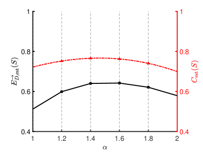
Figure 10: Entanglement estimation results for nonlocal correlations arising from non-maximally entangled states. The experimental setting is given by $\delta=\pi/6,\theta_{1}=\pi/2,\theta_{2}=\pi/6$ and $\theta_{3}=-\pi/6$. We depict the entanglement estimation results when using different $\alpha$-CHSH Bell expressions. We plot the estimated values of one-way distillable entanglement and concurrence with the black solid line and the red dashed line, respectively.

To see when better entanglement estimation is obtained with $\alpha>1$ for the family of non-maximally entangled states, we analytically derive the condition of the underlying system for the measure of concurrence. Using Eq. (17), we have the following result.

Theorem 2.

In a Bell test experiment, suppose the underlying state of the system takes the form of Eq. (22), and the observables take the form of Eq. (21). For concurrence estimation solely from the violation values of $\alpha$-CHSH Bell inequalities, if $\theta_{1},\theta_{2},\theta_{3}$ and $\delta$ satisfy

$$\sin 2\delta\sin\theta_{1}(\sin\theta_{2}-\sin\theta_{3})+\cos\theta_{2}(\sqrt{2}+1+\cos\theta_{1})+\cos\theta_{3}(\sqrt{2}+1-\cos\theta_{1})>2(1+\sqrt{2}),$$ (23)

then there exists $\alpha>1$, where a better estimation of $C_{\rm est}(S)$ can be obtained by using the $\alpha$-CHSH inequality parameterized by this value than by using the original CHSH inequality (corresponding to $\alpha=1$).

Theorem 2 analytically confirms the nonlocality depicted by the original CHSH Bell value does not always provide the concurrence estimation that approaches the real value most. When a fixed nonlocal behavior is given in a CHSH Bell test, when the non-maximally entangled state parameter $\delta$ in Eq. (22) and measurement parameters $\theta_{1},\theta_{2},\theta_{3}$ in Eq. (21) satisfy Eq. (23), it is feasible to take a CHSH-type Bell value with $\alpha>1$ to estimate concurrence of the state. We leave the proof of Theorem 2 in Appendix C.

Example. We take a special set of parameters in Eq. (23) for an example. Suppose $\theta_{1}=\pi/2$ and $\theta_{3}=-\theta_{2}$, which resemble the optimal measurements in Eq. (12) in form. Under this setting, we derive an explicit expression of $\alpha_{0}>1$, such that the estimation $C_{\rm est}(S)$ is optimal when taking $\alpha=\alpha_{0}$ in the CHSH inequality. When $0<\theta_{2}<\pi/4$, any non-maximally entangled state that satisfies

$$\sin 2\delta>(1+\sqrt{2})\frac{1-\cos\theta_{2}}{\sin\theta_{2}}$$ (24)

permits a better concurrence estimation characterizing with some $\alpha>1$. When the state and measurements satisfy the condition in Eq. (24), one obtains the optimally estimated concurrence when the parameter $\alpha$ equals

$$\alpha_{C}^{*}=\frac{1}{2}\left(T-\frac{1}{T}\right)>1,$$ (25)

where we denote $T=\frac{\sin 2\delta\sin\theta_{2}}{1-\cos\theta_{2}}$. The optimally estimated concurrence is then given by

$$C_{\rm est}|_{\alpha_{C}^{*}}=\frac{1-\cos\theta_{2}}{2}(T^{2}+1).$$ (26)

It is worth mentioning that if we have the additional assumption that the underlying state is a pair of qubits, we can analytically derive a more accurate estimation result of concurrence. We leave the detailed conclusions and examples in Appendix C.

V.2 Werner states

In the second simulation model, we consider the set of Werner states,

$$\rho_{\mathrm{W}}(p)=(1-p)\outerproduct{\Phi^{+}}{\Phi^{+}}+p\frac{I}{4},$$ (27)

where we write $\ket{\Phi^{+}}=(\ket{00}+\ket{11})/\sqrt{2}$. The Werner state is entangled when $p<2/3$. Similarly, for the family of Werner states, there are examples that a non-trivial choice of $\alpha$-CHSH expression gives a better estimation result. In Fig. 11, we present such an example. In the simulation, the underlying system is parameterized by $p=0.05$, and the measurements are parameterized by $\theta_{1}=\pi/2,\theta_{2}=\pi/6$ and $\theta_{3}=-\pi/6$. The optimal estimation of negative conditional entropy is obtained with the value of $\alpha$ roughly in the range of $[1.2,1.4]$, while the optimal estimation of concurrence is obtained when $\alpha\in[1,1.2]$. We derive an analytical result for the feasible region of state and measurement parameters that permits a better concurrence estimation for a non-trivial value of $\alpha>1$.

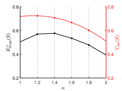
Figure 11: Entanglement estimation results for nonlocal correlations arising from Werner states. The experimental setting is given by $p=0.05,\theta_{1}=\pi/2,\theta_{2}=\pi/6$, and $\theta_{3}=-\pi/6$. We depict the entanglement estimation results using different $\alpha$-CHSH Bell expressions. We plot the estimated values of one-way distillable entanglement and concurrence with the black solid line and the red dashed line, respectively.

Theorem 3.

In a Bell test experiment, suppose the underlying state of the system takes the form of Eq. (27), and the observables take the form of Eq. (21). For concurrence estimation solely from the violation values of $\alpha$-CHSH Bell inequalities, if $\theta_{1},\theta_{2},\theta_{3}$ and $p$ satisfy

$$(1-p)[\sin\theta_{1}(\sin\theta_{2}-\sin\theta_{3})+\cos\theta_{2}(\sqrt{2}+1+\cos\theta_{1})+\cos\theta_{3}(\sqrt{2}+1-\cos\theta_{1})]>2(1+\sqrt{2}),$$ (28)

then there exists $\alpha>1$, where a better estimation of $C_{\rm est}(S)$ can be obtained by using the $\alpha$-CHSH inequality parameterized by this value than by using the original CHSH inequality (corresponding to $\alpha=1$).

Theorem 3 indicates that the nonlocality depicted by the original CHSH Bell value does not always provide the most accurate concurrence estimation of Werner states. In a Bell test experiment, for Werner states parameter $p$ in Eq. (27) and measurement parameters $\theta_{1},\theta_{2},\theta_{3}$ in Eq. (21) satisfy Eq. (28), it is helpful to take a CHSH-type Bell value with $\alpha>1$ to estimate concurrence of the Werner state. We leave the proof and discussion of Theorem 3 in Appendix C.

Example. As a special example, we take the measurements setting in Eq. (23) with $\theta_{1}=\pi/2,\theta_{3}=-\theta_{2}$, the same one as we use for the case study of non-maximally entangled states. For $0<\theta_{2}<\pi/4$, any Werner state in Eq. (27) with $p$ satisfying

$$p<1-\frac{1}{(\sqrt{2}-1)\sin\theta_{2}+\cos\theta_{2}}$$ (29)

promises a better estimation result of $C_{\rm est}$ by using an $\alpha$-CHSH expression with $\alpha>1$ in comparison with $\alpha=1$. The right hand side of Eq. (29) is upper bounded by $1-(\sqrt{2}+1)/(\sqrt{4+2\sqrt{2}})\doteq 0.0761$. That is, only a Werner state with $p\lesssim 0.0761$ is possible to yield the condition in Theorem 3. Denote $T=\frac{(1-p)\sin\theta_{2}}{1-(1-p)\cos\theta_{2}}$. Then for the underlying system of a Werner state and measurements satisfying Eq. (29), the concurrence estimation result reaches its optimal value with parameter $\alpha$

$$\alpha_{C}^{*}=\frac{1}{2}\left(T-\frac{1}{T}\right)>1,$$ (30)

and the estimation result is

$$C_{\rm est}|_{\alpha_{C}^{*}}=1-\frac{p(2-p)}{2[1-(1-p)\cos\theta_{2}]}.$$ (31)

Similarly, with an additional assumption on system dimension, we can obtain a more accurate concurrence estimation result. We leave the details in Appendix C.

VI Conclusions and discussion

In this work, we study entanglement quantification via nonlocality, where we consider several entanglement measures for a family of generalized CHSH-type expressions. This family of Bell expressions allows us to effectively reduce the dimension of an unknown system to a pair of qubits, leading to results for particular entanglement measures like concurrence, entanglement of formation, and one-way distillable entanglement. Under this framework, we also investigate the interplay among entanglement, measurement incompatibility, and nonlocality. While entanglement and measurement incompatibility are both necessary conditions for a nonlocal behavior, under a given nonlocal behavior, their interplay can be subtler than a simple trade-off relation. Given a Bell value, the measurements that require the minimum entanglement are not the most incompatible measurements in general. In addition, we also apply the entanglement quantification results in realistic scenarios. For non-maximally entangled states and Werner states, we analytically show that there exist state and measurements settings where a general CHSH Bell expression with $\alpha>1$ leads to better concurrence estimation of the underlying state than the original CHSH expression.

When quantifying entanglement from nonlocality, the estimation results highly depend on the specific entanglement measures. Before our work, there are similar investigations focusing on different entanglement measures [20, 22]. A natural question is hence how nonlocality reflects various entanglement properties. Particularly, novel results may arise from high-dimensional entanglement and Bell expressions with multiple inputs and outputs, such as the study of Peres conjecture.

In studying the interplay of entanglement and measurement incompatibility under a given nonlocal behavior, we make some additional assumptions on the measurement observables to ease the quantification of measurement incompatibility. In the sense of a fully device-independent discussion, one may consider other incompatibility measures, such as the robustness of measurement incompatibility [39]. Despite the freedom in measuring entanglement and measurement incompatibility, we believe our results unveil the subtlety of the interplay between these nonclassical notions, where more incompatible measurements may not compensate for the absence of entanglement and vice versa. From a resource-theoretic perspective, our results may indicate restrictions on the resource transformation between entanglement and measurement incompatibility in the sense of Bell nonlocality.

When applying our results to experiments, one may consider the practical issues in more detail. For instance, the problem of entanglement estimation via nonlocality can be generalized to the one-shot regime, where one considers dilution and distillation processes with a finite number of possibly non-i.i.d. quantum states. Notably, the results in Ref. [22] provide an approach to estimating one-shot one-way distillable entanglement via nonlocality, and the techniques in Ref. [40] may be applicable to the estimation of one-shot entanglement cost. We leave research in this direction for future works.

VII Acknowledgement

This work was supported by the National Natural Science Foundation of China Grant No. 12174216.

Y.Z. and X.Z. contributed equally to this work.

Appendix A Reductions of the original optimization problem

In Sec. III, we reduce the original optimization problem, including the essential steps of using Jordan’s lemma to bypass the dimension problem and reducing a general two-qubit state to the Bell-diagonal state. Here we explain the two steps in detail.

A.1 Jordan’s lemma

We apply Jordan’s lemma to bypass the system dimension problem. The description of Jordan’s lemma is given below, with the proof can be found in [34].

Lemma 3.

Suppose $\hat{A}_{0}$ and $\hat{A}_{1}$ are two Hermitian operators with eigenvalues $\pm 1$ that act on a Hilbert space with a finite or countable dimension, $\mathcal{H}$. Then there exists a direct-sum decomposition of the system, $\mathcal{H}=\bigoplus\mathcal{H}^{\mu}$, such that $\hat{A}_{0}=\bigoplus\hat{A}_{0}^{\mu}$, $\hat{A}_{1}=\bigoplus\hat{A}_{1}^{\mu}$, $\hat{A}_{0}^{\mu},\hat{A}_{1}^{\mu}\in\mathcal{L}(\mathcal{H}^{\mu})$, where the sub-systems satisfy $\operatorname{dim}\mathcal{H}^{\mu}\leq 2,\forall{\mu}$.

Without loss of generality, we can treat the two measurement observables on each side as projective ones with eigenvalues $\pm 1$. Jordan’s lemma guarantees that the two possible observables measured by Alice can be represented as

$$\hat{A}_{x}=\sum_{\mu}\hat{\Pi}^{\mu_{A}}\hat{A}_{x}\hat{\Pi}^{\mu_{A}}=\bigoplus_{\mu_{A}}\hat{A}_{x}^{\mu_{A}},$$ (32)

where $x\in\{0,1\}$, $\hat{\Pi}^{\mu_{A}}$ are projectors onto orthogonal subspaces with dimension no larger than $2$, and $\hat{A}_{x}^{\mu_{A}}$ are qubit observables with eigenvalues $\pm 1$. A similar representation applies to Bob’s measurement observables. Due to the direct-sum representation, one can regard the measurement process as first applying a block-dephasing operation to the underlying quantum system. Consequently, one can equivalently regard the measurement process as measuring the following state,

$$\bar{\rho}_{AB}=\sum_{\mu}(\hat{\Pi}^{\mu_{A}}\otimes\hat{\Pi}^{\mu_{B}})\rho_{AB}(\hat{\Pi}^{\mu_{A}}\otimes\hat{\Pi}^{\mu_{B}})=\bigoplus_{\mu}p^{\mu}\rho_{AB}^{\mu}.$$ (33)

Here we relabel the indices with $\mu\equiv\{\mu_{A},\mu_{B}\}$. As the block-dephasing operators act locally on each side, the measurement process does not increase entanglement in the system. Therefore, we can lower-bound the amount of entanglement in the initial system by studying the average amount of entanglement in the ensemble of qubit-pairs, $\{p^{\mu},\rho_{AB}^{\mu}\}$.

Consequently, the expected CHSH Bell value in a test is the linear combination of the Bell values for the qubit pairs, $S=\sum_{\mu}p^{\mu}S^{\mu}$. Note that an observer cannot access to the probability distribution, $p^{\mu}$, and the Bell values for each pair of qubits, $S^{\mu}$, but only the expected Bell value, $S$, hence the final device-independent entanglement quantification result should be a function of $S$. On the other hand, we shall first derive entanglement quantification results for each pair of qubits in the form of $E_{\rm est}(S^{\mu})$. It is thus essential to consider the convexity of the function, $E_{\rm est}$. If the function is not convex in its argument, i.e., $E_{\rm est}(\sum_{\mu}p^{\mu}S^{\mu})$ is not smaller than $\sum_{\mu}p^{\mu}E_{\rm est}(S^{\mu})$, one needs to take the convex closure of $E_{\rm est}$ to obtain a valid lower bound that holds for all possible configurations giving rise to the expected Bell value, $S$.

A.2 Restriction to Bell-diagonal states

Following the route in Fig. 3, the feasible region of the state variables in an entanglement quantification problem can be effectively restricted to the set of Bell-diagonal states on the two qubit systems. We present the following lemma.

Lemma 4.

Suppose the underlying system in a CHSH-type Bell test lies in a two-qubit state, $\rho_{AB}$. Then there exists an LOCC that transforms $\rho_{AB}$ into an ensemble of Bell states, $\rho_{\lambda}$, without changing the expected Bell value.

Proof.

In a CHSH-type Bell test, we transform an arbitrary pair of qubits $\rho_{AB}$ into a Bell-diagonal state $\rho_{\lambda}$ via three steps of LOCC. In each step, We verify that the $\alpha$-CHSH Bell values are equal for the states before and after the transformation with the same measurements.

Step 1: In a CHSH Bell test, Alice and Bob fix their local computational bases, or, the axes of the Bloch spheres on each side. As there are only two observables on each side, one can represent them on the $x-z$ plane of the Bloch sphere without loss of generality. Then Alice and Bob flip their measurement results simultaneously via classical communication with probability $1/2$. This operation can be interpreted as transforming $\rho_{AB}$ into the following state,

$$\rho_{1}=\frac{1}{2}[\rho_{AB}+(\sigma_{2}\otimes\sigma_{2})\rho_{AB}(\sigma_{2}\otimes\sigma_{2})].$$ (34)

To avoid confusion about the subscripts, we use the following convention to denote the Pauli operators in the Appendix,

$$\begin{split}\sigma_{x}&\equiv\sigma_{1},\\ \sigma_{y}&\equiv\sigma_{2},\\ \sigma_{z}&\equiv\sigma_{3}.\end{split}$$ (35)

Under the Bell basis determined by the local computational bases, $\{\ket{\Phi^{+}},\ket{\Psi^{-}},\ket{\Phi^{-}},\ket{\Psi^{+}}\}$, $\rho_{1}$ can be denoted as

$$\rho_{1}=\begin{bmatrix}\lambda_{\Phi^{+}}&l_{1}e^{i\phi_{1}}&0&0\\ l_{1}e^{-i\phi_{1}}&\lambda_{\Psi^{-}}&0&0\\ 0&0&\lambda_{\Psi^{+}}&l_{2}e^{i\phi_{2}}\\ 0&0&l_{2}e^{-i\phi_{2}}&\lambda_{\Phi^{-}}\end{bmatrix}.$$ (36)

It can be verified that the statistics of measuring $\sigma_{i}\otimes\sigma_{j}$ for $i,j=1,3$ are invariant under the operation of $\sigma_{2}\otimes\sigma_{2}$. Thus

$$\Tr[(\sigma_{2}\otimes\sigma_{2})\rho_{AB}(\sigma_{2}\otimes\sigma_{2})(\hat{A}_{x}\otimes\hat{B}_{y})]=\Tr[\rho_{AB}(\hat{A}_{x}\otimes\hat{B}_{y})]$$ (37)

for $\hat{A}_{x}$ and $\hat{B}_{y}$, $x,y=0,1$, which indicates that $\rho_{1}$ and $\rho_{AB}$ share the common Bell value.

Step 2: In this step, we apply LOCC to transform $\rho_{1}$ into a state where the off-diagonal terms on the Bell basis become imaginary numbers. For this purpose, Alice and Bob can each apply a local rotation around the $y$-axes of the Bloch spheres on their own systems,

$$R_{y}(\theta)=\cos{\frac{\theta}{2}}I+i\sin{\frac{\theta}{2}}\sigma_{2}=\left(\begin{smallmatrix}\cos{\frac{\theta}{2}}&\sin{\frac{\theta}{2}}\\ -\sin{\frac{\theta}{2}}&\cos{\frac{\theta}{2}}\end{smallmatrix}\right),$$ (38)

with its action on a general observable residing in the $x-z$ plane given by

$$R_{y}(\theta)(\cos\gamma\sigma_{1}+\sin\gamma\sigma_{3})=\cos(\gamma+\frac{\theta}{2})\sigma_{1}+\sin(\gamma+\frac{\theta}{2})\sigma_{3}.$$ (39)

After applying the operation, the resulting state becomes $\rho_{2}=[R_{y}(\alpha)\otimes R_{y}(\beta)]\rho_{1}[R_{y}(-\alpha)\otimes R_{y}(-\beta)]$, where the off-diagonal terms undergo the following transformations,

$$l_{1}e^{i\phi_{1}}\rightarrow\frac{1}{2}(\lambda_{\Phi^{+}}-\lambda_{\Psi^{-}})\sin(\alpha-\beta)+l_{1}\cos\phi_{1}\cos(\alpha-\beta)+l_{1}\sin\phi_{1}i,$$ (40)

$$l_{2}e^{i\phi_{2}}\rightarrow\frac{1}{2}(\lambda_{\Phi^{-}}-\lambda_{\Psi^{+}})\sin(\alpha+\beta)+l_{2}\cos\phi_{2}\cos(\alpha+\beta)+l_{2}\sin\phi_{2}i.$$ (41)

By choosing $\alpha$ and $\beta$ properly, the real parts in the off-diagonal terms of $\rho_{2}$ can be eliminated. Similarly, as in the Step 1, the measurement of $\sigma_{i}\otimes\sigma_{j}$ for $i,j=1,3$ remains invariant under local rotations around the $y$-axes, which indicates $\rho_{2}$ and $\rho_{1}$ give the same Bell value under the same measurements.

Step 3: Note that $\rho_{2}$ and $\rho_{2}^{*}$ give the same Bell value under the given measurements,

$$\Tr[\rho_{2}(\sigma_{i}\otimes\sigma_{j})]=\Tr[\rho_{2}^{*}(\sigma_{i}\otimes\sigma_{j})],i,j=1,3.$$ (42)

Hence without loss of generality, one can take the underlying state in the Bell test as $\rho_{\lambda}=(\rho_{2}+\rho_{2}^{*})/2$, which is a Bell-diagonal state. ∎

Based on the above simplification, we represent Eq. (9) under Bell-diagonal states, which leads to the following lemma.

Lemma 5.

The maximal value of the $\alpha$-CHSH expression in Eq. (2) for a Bell-diagonal state shown in Eq. (10), $\rho_{\lambda}$, is given by

$$S=2\sqrt{\alpha^{2}(\lambda_{1}+\lambda_{2}-\lambda_{3}-\lambda_{4})^{2}+(\lambda_{1}-\lambda_{2}+\lambda_{3}-\lambda_{4})^{2}},$$ (43)

where $\lambda_{i}$ is the $i$-th largest eigenvalue of $\rho_{\lambda}$.

Proof.

In an $\alpha$-CHSH Bell test, measurements corresponding to non-degenerate Pauli observables can be expressed as

$$\hat{A_{x}}=\vec{a}_{x}\cdot\vec{\sigma},$$ (44)

$$\hat{B_{y}}=\vec{b}_{y}\cdot\vec{\sigma},$$ (45)

where $\vec{\sigma}=(\sigma_{1},\sigma_{2},\sigma_{3})$ are three Pauli matrices, and $\vec{a}_{x}=(a_{x}^{1},a_{x}^{2},a_{x}^{3})$ and $\vec{b}_{y}=(b_{y}^{1},b_{y}^{2},b_{y}^{3})$ are unit vectors for $x,y=0,1$. A Bell-diagonal state shown in Eq. (10) can be expressed on the Hilbert-Schmidt basis as

$$\rho_{\lambda}=\frac{1}{4}\left(I+\sum_{i,j=1}^{3}T_{\lambda,ij}\sigma_{i}\otimes\sigma_{j}\right),$$ (46)

where

$$T_{\lambda}=\begin{bmatrix}(\lambda_{1}+\lambda_{3})-(\lambda_{2}+\lambda_{4})&0&0\\ 0&(\lambda_{3}+\lambda_{2})-(\lambda_{1}+\lambda_{4})&0\\ 0&0&(\lambda_{1}+\lambda_{2})-(\lambda_{3}+\lambda_{4})\end{bmatrix}$$ (47)

is a diagonal matrix. The $\alpha$-CHSH expression in Eq. (2) can be expressed in terms of $T_{\lambda}$ as

$$\Tr\left\{\alpha\rho_{\lambda}(\vec{a}_{0}\cdot\vec{\sigma})\otimes[(\vec{b}_{0}+\vec{b}_{1})\cdot\vec{\sigma}]+\rho_{\lambda}(\vec{a}_{1}\cdot\sigma)\otimes[(\vec{b}_{0}-\vec{b}_{1})\cdot\vec{\sigma}]\right\}$$ (48)

$$= \alpha[\vec{a}_{0}\cdot T_{\lambda}(\vec{b}_{0}+\vec{b}_{1})]+[\vec{a}_{1}\cdot T_{\lambda}(\vec{b}_{0}-\vec{b}_{1})].$$

Following the method in Ref. [41], we introduce a pair of normalized orthogonal vectors, $\vec{c}_{0}$ and $\vec{c}_{1}$,

$$\vec{b}_{0}+\vec{b}_{1}=2\cos\theta\vec{c}_{0},$$ (49)

$$\vec{b}_{0}-\vec{b}_{1}=2\sin\theta\vec{c}_{1}$$ (50)

where $\theta\in[0,\pi/2]$. This gives the maximal $\alpha$-CHSH Bell value,

$$S = =\max_{\vec{a}_{0},\vec{a}_{1},\vec{c}_{0},\vec{c}_{1},\theta}2\alpha\cos\theta(\vec{a}_{0}\cdot T_{\lambda}\vec{c}_{0})+2\sin\theta(\vec{a}_{1}\cdot T_{\lambda}\vec{c}_{1}).$$ (51)

The maximization of the Bell value is taken over parameters $\vec{a}_{x},\vec{b}_{y}$ for $x,y=0,1$, with the parameters $\lambda_{i}$ fixed. We obtain

$$S =\max_{\vec{c}_{0},\vec{c}_{1},\theta}2\alpha\cos\theta|T_{\lambda}\vec{c}_{0}|+2\sin\theta|T_{\lambda}\vec{c}_{1}|$$ (52)

$$=\max_{\vec{c}_{0},\vec{c}_{1}}2\sqrt{\alpha^{2}|T_{\lambda}\vec{c}_{0}|^{2}+|T_{\lambda}\vec{c}_{1}|^{2}},$$

where the first equality in Eq. (52) is saturated when $\vec{a}_{x}=T_{\lambda}\vec{c}_{x}/|T_{\lambda}\vec{c}_{x}|,x=0,1$, and the second inequality is saturated when $\tan\theta=|T_{\lambda}\vec{c}_{1}|/(\alpha|T_{\lambda}\vec{c}_{0}|)$. Since $\alpha>1$ and $\vec{c}_{0}$ and $\vec{c}_{1}$ are orthonormal vectors, the maximum of the second line in Eq. (52) is obtained when $|T_{\lambda}\vec{c}_{0}|$ and $|T_{\lambda}\vec{c}_{1}|$ equal to the absolute values of the largest and the second largest eigenvalues of $T_{\lambda}$, respectively. Without loss of generality, we assume $\lambda_{1}\geq\lambda_{2}\geq\lambda_{3}\geq\lambda_{4}$ in $\rho_{\lambda}$. This leads to the ordering of the absolute values of the elements of $T_{\lambda}$,

$$\begin{split}|T_{\lambda,33}|&=|(\lambda_{1}-\lambda_{4})+(\lambda_{2}-\lambda_{3})|\geq|(\lambda_{1}-\lambda_{4})-(\lambda_{2}-\lambda_{3})|=|T_{\lambda,11}|,\\ |T_{\lambda,11}|&=|(\lambda_{3}-\lambda_{4})+(\lambda_{1}-\lambda_{2})|\geq|(\lambda_{3}-\lambda_{4})-(\lambda_{1}-\lambda_{2})|=|T_{\lambda,22}|.\end{split}$$ (53)

Thus, the second line in Eq. (52) reaches its maximum when $|\vec{c}_{0}|=(0,0,1)^{T}$ and $|\vec{c}_{1}|=(1,0,0)^{T}$. Therefore, for any given Bell-diagonal state $\rho_{\lambda}$ in Eq. (10), the maximal $\alpha$-CHSH Bell value is

$$S=2\sqrt{\alpha^{2}(\lambda_{1}+\lambda_{2}-\lambda_{3}-\lambda_{4})^{2}+(\lambda_{1}-\lambda_{2}+\lambda_{3}-\lambda_{4})^{2}},$$ (54)

where measurements for $\rho_{\lambda}$ to achieve the maximal Bell value, i.e., optimal measurements, are given by

$$\begin{gathered}\hat{A}_{0}=\pm\sigma_{z},\\ \hat{A}_{1}=\pm\sigma_{x},\\ \hat{B}_{0}=\pm\cos\theta\sigma_{z}\pm\sin\theta\sigma_{x},\\ \hat{B}_{1}=\pm\cos\theta\sigma_{z}\mp\sin\theta\sigma_{x},\end{gathered}$$ (55)

or

$$\begin{gathered}\hat{A}_{0}=\pm\sigma_{z},\\ \hat{A}_{1}=\mp\sigma_{x},\\ \hat{B}_{0}=\pm\cos\theta\sigma_{z}\mp\sin\theta\sigma_{x},\\ \hat{B}_{1}=\pm\cos\theta\sigma_{z}\pm\sin\theta\sigma_{x},\end{gathered}$$ (56)

with $\tan\theta=(\lambda_{1}-\lambda_{2}+\lambda_{3}-\lambda_{4})/[\alpha(\lambda_{1}+\lambda_{2}-\lambda_{3}-\lambda_{4})]$. ∎

From the proof, we see that any Bell-diagonal state $\rho_{\lambda}$ in Eq. (10) reaches its maximal Bell value of Eq. (2) when measurements are taken in the form Eq. (55) or Eq. (56). In other words, measurements in Eq. (55) and Eq. (56) are the optimal measurements for $\rho_{\lambda}$ that yield the largest $\alpha$-CHSH Bell value. To solve the simplified entanglement estimation problem in Eq. (9) for Bell-diagonal states, we need to solve the optimal measurements first. Given a general pair of qubits $\rho_{AB}$, the maximal $\alpha$-CHSH Bell value $S$ for $\rho_{AB}$ is expressed as a function of $T_{ij}$,

$$S=[2(\alpha^{2}+1)(T_{11}^{2}+T_{13}^{2}+T_{31}^{2}+T_{33}^{2})+2(\alpha^{2}-1)\sqrt{(T_{11}^{2}-T_{13}^{2}+T_{31}^{2}-T_{33}^{2})^{2}+4(T_{11}+T_{13}+T_{31}+T_{33})^{2}}]^{1/2},$$ (57)

where $T_{ij}=\Tr[\rho_{AB}(\sigma_{i}\otimes\sigma_{j})]$ is the coefficient of $\rho_{AB}$ under Hilbert-Schmidt basis. When $\rho_{AB}$ is Bell-diagonal, Eq. (57) degenerates to Eq. (43).

Appendix B Proof of the lower bound of concurrence

In this section, we prove the analytical concurrence estimation result via the $\alpha$-CHSH Bell value. Here we restrict the underlying state as a pair of qubits.

Theorem 4.

Suppose the underlying quantum state is a pair of qubits. For a given $\alpha$-CHSH expression in Eq. (2) parametrized by $\alpha$, if the Bell value is $S$, then the amount of concurrence in the underlying state can be lower-bounded,

$$C(\rho_{AB})\geq\sqrt{\frac{S^{2}}{4}-\alpha^{2}}.$$ (58)

The equality can be saturated when measuring a Bell-diagonal state in Eq. (10) with eigenvalues

$$\begin{gathered}\lambda_{1}=\frac{1}{2}+\frac{1}{2}\sqrt{\frac{S^{2}}{4}-\alpha^{2}},\\ \lambda_{2}=\frac{1}{2}-\frac{1}{2}\sqrt{\frac{S^{2}}{4}-\alpha^{2}},\\ \lambda_{3}=\lambda_{4}=0,\end{gathered}$$ (59)

using measurements in Eq. (12) with $\theta=\arctan(\frac{1}{\alpha}\sqrt{\frac{S^{2}}{4}-\alpha^{2}})$.

Proof.

Given any Bell value $S\in(2\alpha,2\sqrt{1+\alpha^{2}}]$, we aim to determine the least amount of concurrence that is required to support the Bell value, $S$. We solve the simplified optimization problem in Eq. (9), restricting the underlying state as a Bell-diagonal state in Eq. (10) and taking the objective entanglement measure as $C(\cdot)$,

$$\begin{split}C_{\rm est}&=\underset{\lambda_{i},i=1,2,3,4}{\text{min}}\max\{0,2\lambda_{1}-1\},\\ \text{s.t.}\quad S&=2\sqrt{\alpha^{2}(\lambda_{1}+\lambda_{2}-\lambda_{3}-\lambda_{4})^{2}+(\lambda_{1}-\lambda_{2}+\lambda_{3}-\lambda_{4})^{2}},\\ \lambda_{1}&\geq\lambda_{2}\geq\lambda_{3}\geq\lambda_{4},\\ 1&=\sum_{i=1}^{4}\lambda_{i},\lambda_{i}\geq 0\;,i=1,2,3,4.\end{split}$$ (60)

We first reduce the number of variables to simplify the optimization in Eq. (60). Since the variables in Eq. (60) are not independent with each other, we express variables $\lambda_{1}$ and $\lambda_{4}$ as functions of variables $\lambda_{2}$ and $\lambda_{3}$,

$$\lambda_{\max}=\lambda_{1}=\frac{1}{2}-\frac{1}{\alpha^{2}+1}(\alpha^{2}\lambda_{2}+\lambda_{3})+\frac{1}{\alpha^{2}+1}\sqrt{\frac{S^{2}(\alpha^{2}+1)}{16}-\alpha^{2}(\lambda_{2}-\lambda_{3})^{2}},$$ (61)

$$\lambda_{\min}=\lambda_{4}=\frac{1}{2}-\frac{1}{\alpha^{2}+1}(\lambda_{2}+\alpha^{2}\lambda_{3})-\frac{1}{\alpha^{2}+1}\sqrt{\frac{S^{2}(\alpha^{2}+1)}{16}-\alpha^{2}(\lambda_{2}-\lambda_{3})^{2}}.$$ (62)

The non-negativity of $\lambda_{\min}$ in Eq. (62) restricts $\lambda_{2}$ and $\lambda_{3}$ outside an ellipse,

$$\left(\lambda_{2}-\frac{1}{2}\right)^{2}+\alpha^{2}\left(\lambda_{3}-\frac{1}{2}\right)^{2}\geq\frac{S^{2}}{16},$$ (63)

and the fact that $\lambda_{4}$ in Eq. (62) is the smallest among all $\lambda_{i}$ restricts $\lambda_{2}$ and $\lambda_{3}$ inside an ellipse,

$$\lambda_{2}^{2}+(4\alpha^{2}+1)\lambda_{3}+2\lambda_{2}\lambda_{3}-\lambda_{2}-(2\alpha^{2}+1)\lambda_{3}\leq\frac{S^{2}}{16}-\frac{\alpha^{2}+1}{4}.$$ (64)

With the above derivations, the optimization in Eq. (60) can be rewritten with independent variables $\lambda_{2}$ and $\lambda_{3}$ as

$$\begin{split}C_{\rm est}&=\underset{\lambda_{2},\lambda_{3}}{\text{min}}2\lambda_{1}-1,\\ \text{s.t.}\quad\lambda_{1}&=\frac{1}{2}-\frac{1}{\alpha^{2}+1}(\alpha^{2}\lambda_{2}+\lambda_{3})+\frac{1}{\alpha^{2}+1}\sqrt{\frac{S^{2}(\alpha^{2}+1)}{16}-\alpha^{2}(\lambda_{2}-\lambda_{3})^{2}},\\ 0&\leq(\lambda_{2}-\frac{1}{2})^{2}+\alpha^{2}(\lambda_{3}-\frac{1}{2})^{2}-\frac{S^{2}}{16},\\ 0&\geq\lambda_{2}^{2}+(4\alpha^{2}+1)\lambda_{3}+2\lambda_{2}\lambda_{3}-\lambda_{2}-(2\alpha^{2}+1)\lambda_{3}-(\frac{S^{2}}{16}-\frac{\alpha^{2}+1}{4}),\\ \lambda_{1}&\geq\lambda_{2}\geq\lambda_{3},\\ 0&\leq\lambda_{2},\lambda_{3},\lambda_{2}+\lambda_{3}\leq 1.\end{split}$$ (65)

The optimization in Eq. (65) can be solved analytically, with the global optimal value taken at

$$\begin{gathered}\lambda_{1}=\frac{1}{2}+\frac{1}{2}\sqrt{\frac{S^{2}}{4}-\alpha^{2}},\\ \lambda_{2}=\frac{1}{2}-\frac{1}{2}\sqrt{\frac{S^{2}}{4}-\alpha^{2}},\\ \lambda_{3}=\lambda_{4}=0.\end{gathered}$$ (66)

Therefore the estimated concurrence is lower-bounded,

$$C(\rho_{AB})\geq C_{\rm est}(S)=\sqrt{\frac{S^{2}}{4}-\alpha^{2}}.$$ (67)

The lower bound of Eq. (67) is saturated when the $\alpha$-CHSH Bell value $S$ is obtained by measuring the Bell-diagonal state $\rho_{\lambda}$ with the parameters in Eq. (66) under its optimal measurements. The optimal measurements are in Eq. (55) and Eq. (56) with $\theta=\arctan(\frac{1}{\alpha}\sqrt{\frac{S^{2}}{4}-\alpha^{2}})$. ∎

Appendix C Realistic settings in experiment

In this section, we analyze the realistic settings and analytically derive the condition where a better concurrence estimation can be derived with a tilted CHSH Bell expression. That is, by using the family of $\alpha$-CHSH expressions, a Bell expression with parameter $\alpha>1$ gives a better estimation result than $\alpha=1$. Considering the estimation function, $C_{\rm est}(S)$, as a function parameterized by $\alpha$, then our target is to determine the condition for the following inequalities,

$$\begin{gathered}\frac{\partial C_{\rm est}(S)}{\partial\alpha}|_{\alpha=1}>0,\\ C_{\rm est}(S)|_{\alpha=1}>0.\end{gathered}$$ (68)

The conclusions of Theorem 2 and Theorem 3 can be directly solved from Eq. (68) by substituting the corresponding estimation equation and the $\alpha$-CHSH Bell value.

For a better understanding of Theorem 2, we take $\theta_{1}=\pi/2$ in Eq. (23). With straightforward derivations, we find that when the measurement parameters, $\theta_{2}$ and $\theta_{3}$, satisfy

$$(\sqrt{2}+1)(\cos\theta_{2}+\cos\theta_{3})+(\sin\theta_{2}-\sin\theta_{3})>2(\sqrt{2}+1),$$ (69)

there exists a value of $\delta$ such that $\theta_{1}=\pi/2$, and $\theta_{2},\theta_{3}$ and $\delta$ satisfy the inequality in Eq. (23). In other words, when measurement parameters are set in Eq. (21) with $\theta_{1}=\pi/2$ and $\theta_{2},\theta_{3}$ follow Eq. (69), there exists a proper state, $\ket{\phi_{AB}(\delta)}$, such that concurrence estimation result $C_{\rm est}(S)$ of the $\ket{\phi_{AB}(\delta)}$ for some $\alpha>1$ is larger than that with $\alpha=1$. The conclusion from Eq. (69) also applies to Werner states.

Appendix D Semi-device-independent optimal entanglement estimation

In some scenarios, one may trust the functioning of the source, such as knowing the input states to be pairs of qubits, which can be seen as a semi-device-independent (semi-DI) scenario. With the additional information, one may obtain a better entanglement estimation result. In this section, we compare the performance of this semi-DI scenario with the fully DI scenario under a realistic setting. Suppose the underlying state is a non-maximally entangled state $\ket{\phi_{AB}(\delta)}$ in Eq. (22) with $\delta=0.6$, and the measurements are given by Eq. (21) with $\theta_{1}=\pi/2$ and $\theta_{2}=-\theta_{3}=\pi/2-1.2$. Under this setting, the fully DI and semi-DI concurrence estimation results are illustrated in Fig. 12. The semi-DI estimation, $C_{\rm est,semi-DI}(S)$, is strictly larger than the fully DI estimation, $C_{\rm est,DI}(S)$, for any value of $\alpha>1$. Besides, when $\alpha$ takes the value of $\alpha^{*}_{C}\doteq 2.3973$, $C_{\rm est,semi-DI}|_{\alpha^{*}_{C}}=\sin(1.2)\doteq 0.9320$ rigorously equals to the real system concurrence when $\delta=0.6$.

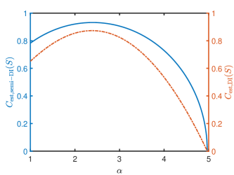
Figure 12: Illustration of the comparison between DI and semi-DI concurrence estimation results. The experimental setting is given by $\delta=0.6,\theta_{1}=\pi/2,\theta_{2}=-\theta_{3}=\pi/2-1.2$. For the estimation results varying in $\alpha>1$, we plot the estimated values from the settings of semi-DI and DI with the blue solid line and the red dashed line, respectively. The semi-DI concurrence estimation with confirmed knowledge of input dimensions is strictly larger than the DI concurrence estimation.

In addition, we also study the condition where a better concurrence estimation result using general $\alpha$-CHSH expressions is obtained under some $\alpha>1$. We present the following theorems for the state families of Werner states and non-maximally entangled states.

Theorem 5.

In a Bell test experiment where the input states are pairs of qubits, suppose the underlying state of the system takes the form of Eq. (22) and the observables take the form of Eq. (21). When $\theta_{1},\theta_{2},\theta_{3}$ and $\delta$ satisfy

$$(\cos\theta_{2}+\cos\theta_{3})[\sin 2\delta\sin\theta_{1}(\sin\theta_{2}-\sin\theta_{3})+(1+\cos\theta_{1})\cos\theta_{2}+(1-\cos\theta_{1})\cos\theta_{3}]>4,$$ (70)

there exists $\alpha>1$, where a better estimation of $C_{\rm est}(S)$ can be obtained by using the $\alpha$-CHSH inequality parameterized by this value than by using the original CHSH inequality (corresponding to $\alpha=1$).

The proof of Theorem 5 is similar to the proof of Theorem 2. Here, we alternatively apply the concurrence estimation result for pairs of qubits input, $C_{\rm est}(S)$ in Eq. (14), to the condition in Eq. (68). To better understand the theorem, we present an example with $\theta_{1}=\pi/2$ in Eq. (70). When

$$\begin{split}\theta_{2}+\theta_{3}&=\arccos(\frac{4}{1+\sqrt{2}k}-1),\\ -\frac{\pi}{4}-\arccos k&<\theta_{3}-\theta_{2}<-\frac{\pi}{4}+\arccos k,\end{split}$$ (71)

where $k\in[\sqrt{2}/2,1)$, there exists $\delta$ such that $\theta_{1}=\pi/2,\theta_{2},\theta_{3}$ and the $\delta$ satisfy Eq. (70). In other words, when measurement parameters are set in Eq. (21) with $\theta_{1}=\pi/2$ and $\theta_{2},\theta_{3}$ following Eq. (71), there exist non-maximally entangled states where a better semi-DI concurrence estimation result is obtained for some $\alpha>1$ in comparison with $\alpha=1$.

In Fig. 12, we observe that under a well-chosen value of $\alpha$, the semi-DI concurrence estimation coincides with the real value. In many semi-DI CHSH Bell tests, the existence of $\alpha$ that yields an accurate estimation of state concurrence is ubiquitous. Theorem 1 indicates that under the assumption of qubit inputs, the lower bound of concurrence in Eq. (14) can be saturated at any non-maximally entangled state $\ket{\phi_{AB}(\delta)}$, once the Bell value is obtained by the optimal measurements of the $\ket{\phi_{AB}(\delta)}$. In fact, earlier research indicates that the observables,

$$\begin{split}\hat{A}_{0}&=\pm\sigma_{z},\\ \hat{A}_{1}&=\sigma_{x},\\ \hat{B}_{0}&=\pm\cos\theta\sigma_{z}+\sin\theta\sigma_{x},\\ \hat{B}_{1}&=\pm\cos\theta\sigma_{z}-\sin\theta\sigma_{x},\end{split}$$ (72)

with $\tan\theta=\sin 2\delta/\alpha$, are the optimal measurements of $\ket{\phi_{AB}}$ with any fixed $\alpha$ [27] . The form of observables in Eq. (72) coincides with our initialization in Eq. (21) when $\theta_{1}=\pi/2,\theta_{2}+\theta_{3}=0,0<\theta_{2}<\pi/4$. In this case, any non-maximally entangled state $\ket{\phi_{AB}(\delta)}$ with $\delta$ satisfying $\sin 2\delta>\tan\theta_{2}$ reaches its optimal concurrence estimation when $\alpha$ takes the value of

$$\alpha^{*}_{C}=\frac{\sin 2\delta}{\tan\theta_{2}},$$ (73)

and the optimal semi-DI estimation value is

$$C_{\rm est}|_{\alpha^{*}_{C},\rm semi-DI}=C(\ket{\phi_{AB}}).$$ (74)

Theorem 6.

In a Bell test experiment where the input states are pairs of qubits, suppose the underlying state of the system takes the form of Eq. (27) and the observables take the form of Eq. (21). When $\theta_{1},\theta_{2},\theta_{3}$ and $p$ satisfy

$$(1-p)^{2}(\cos\theta_{2}+\cos\theta_{3})\cdot[\sin\theta_{1}(\sin\theta_{2}-\sin\theta_{3})+(1+\cos\theta_{1})\cos\theta_{2}+(1-\cos\theta_{1})\cos\theta_{3}]>4,$$ (75)

there exists $\alpha>1$, where a better estimation of $C_{\rm est}(S)$ can be obtained by using the $\alpha$-CHSH inequality parameterized by this value than by using the original CHSH inequality (corresponding to $\alpha=1$).

The proof of Theorem 6 is similar to the proof of Theorem 3. Theorem 6 is derived from the concurrence estimation result for pairs of qubits input, $C_{\rm est}(S)$ in Eq. (14), and the condition in Eq. (68). Here we take $\theta_{1}=\pi/2$ for convenience, when $\theta_{2}$ and $\theta_{3}$ satisfy Eq. (71) for $k\in[\sqrt{2}/2,1)$, there exists Werner states $\rho_{W}$ such that, the semi-DI concurrence estimation under the settings performs better when taking an $\alpha>1$ CHSH-type Bell expression compared with $\alpha=1$.

We further interpret Theorem 6 via a special example. In a semi-DI CHSH Bell test, if measurements in Eq. (21) are set with $\theta_{1}=\pi/2,\theta_{2}+\theta_{3}=0,0<\theta_{2}<\pi/4$, then any Werner state $\rho_{W}$ with parameter $p$,

$$p<1-\frac{1}{\sqrt{\sqrt{2}\cos\theta_{2}\cos(\theta_{2}-\pi/4)}},$$ (76)

promises a better concurrence estimation when taking an $\alpha>1$ CHSH-type Bell expression compared with $\alpha=1$. The right hand side (RHS) of Eq. (76) is no large than $0.0896$, which implies only Werner state with $p\lesssim 0.0896$ is possible to fit in the condition in Theorem 6. It is worth mentioning that for any $0<\theta_{2}<\pi/4$, the RHS of Eq. (76) is strictly larger than the RHS of Eq. (29). It allows a wide choice of Werner states to promise a better estimation when taking an $\alpha>1$ CHSH-type Bell expression compared with $\alpha=1$ in the semi-DI experiment. In a semi-DI system with the Werner state and measurements satisfying Eq. (76), the semi-DI concurrence estimation reaches the optimal when the CHSH Bell value is taken at $\alpha$ equals to

$$\alpha^{*}_{C}=\frac{(1-p)^{2}\cos\theta_{2}\sin\theta_{2}}{1-(1-p)^{2}\cos^{2}\theta_{2}}$$ (77)

and the optimal semi-DI estimation value is

$$C_{\rm est}|_{\alpha^{*}_{C},{\rm semi-DI}}=\frac{(1-p)\sin\theta_{2}}{\sqrt{1-(1-p)^{2}\cos^{2}\theta_{2}}}.$$ (78)

References

- Einstein et al. [1935] A. Einstein, B. Podolsky, and N. Rosen, Phys. Rev. 47, 777 (1935), URL https://link.aps.org/doi/10.1103/PhysRev.47.777.
- Bell [1964] J. S. Bell, Phys. Phys. Fiz. 1, 195 (1964), URL https://link.aps.org/doi/10.1103/PhysicsPhysiqueFizika.1.195.
- Clauser et al. [1969] J. F. Clauser, M. A. Horne, A. Shimony, and R. A. Holt, Phys. Rev. Lett. 23, 880 (1969), URL https://link.aps.org/doi/10.1103/PhysRevLett.23.880.
- Schrödinger [1935] E. Schrödinger, in Mathematical Proceedings of the Cambridge Philosophical Society (Cambridge University Press, 1935), vol. 31, pp. 555–563.
- Cirel’son [1980] B. S. Cirel’son, Letters in Mathematical Physics 4, 93 (1980), URL https://doi.org/10.1007/BF00417500.
- Gühne and Tóth [2009] O. Gühne and G. Tóth, Phys. Rep. 474, 1 (2009), URL https://www.sciencedirect.com/science/article/pii/S0370157309000623.
- Horodecki et al. [2009] R. Horodecki, P. Horodecki, M. Horodecki, and K. Horodecki, Rev. Mod. Phys. 81, 865 (2009), URL https://link.aps.org/doi/10.1103/RevModPhys.81.865.
- Curty et al. [2004] M. Curty, M. Lewenstein, and N. Lütkenhaus, Phys. Rev. Lett. 92, 217903 (2004), URL https://link.aps.org/doi/10.1103/PhysRevLett.92.217903.
- Jozsa and Linden [2003] R. Jozsa and N. Linden, Proc. Math. Phys. Eng. Sci. 459, 2011 (2003), URL https://royalsocietypublishing.org/doi/10.1098/rspa.2002.1097.
- Giovannetti et al. [2011] V. Giovannetti, S. Lloyd, and L. Maccone, Nat. Photonics 5, 222 (2011), URL https://www.nature.com/articles/nphoton.2011.35.
- Vedral et al. [1997] V. Vedral, M. B. Plenio, M. A. Rippin, and P. L. Knight, Phys. Rev. Lett. 78, 2275 (1997), URL https://link.aps.org/doi/10.1103/PhysRevLett.78.2275.
- Lo and Chau [1999] H.-K. Lo and H. F. Chau, Science 283, 2050 (1999), URL https://www.science.org/doi/10.1126/science.283.5410.2050.
- Shor and Preskill [2000] P. W. Shor and J. Preskill, Phys. Rev. Lett. 85, 441 (2000), URL https://link.aps.org/doi/10.1103/PhysRevLett.85.441.
- Bennett et al. [1996] C. H. Bennett, D. P. DiVincenzo, J. A. Smolin, and W. K. Wootters, Phys. Rev. A 54, 3824 (1996), URL https://link.aps.org/doi/10.1103/PhysRevA.54.3824.
- Raymer et al. [1994] M. G. Raymer, M. Beck, and D. McAlister, Phys. Rev. Lett. 72, 1137 (1994), URL https://link.aps.org/doi/10.1103/PhysRevLett.72.1137.
- Leonhardt [1996] U. Leonhardt, Phys. Rev. A 53, 2998 (1996), URL https://link.aps.org/doi/10.1103/PhysRevA.53.2998.
- Leonhardt [1997] U. Leonhardt, Measuring the quantum state of light, vol. 22 (Cambridge university press, 1997).
- Mayers and Yao [1998] D. Mayers and A. Yao, in Proceedings of the 39th Annual Symposium on Foundations of Computer Science (IEEE Computer Society, Washington, DC, USA, 1998), FOCS ’98, pp. 503–509, ISBN 0-8186-9172-7, URL http://dl.acm.org/citation.cfm?id=795664.796390.
- Acín et al. [2007] A. Acín, N. Brunner, N. Gisin, S. Massar, S. Pironio, and V. Scarani, Phys. Rev. Lett. 98, 230501 (2007), URL https://link.aps.org/doi/10.1103/PhysRevLett.98.230501.
- Moroder et al. [2013] T. Moroder, J.-D. Bancal, Y.-C. Liang, M. Hofmann, and O. Gühne, Phys. Rev. Lett. 111, 030501 (2013), URL https://link.aps.org/doi/10.1103/PhysRevLett.111.030501.
- Arnon-Friedman and Yuen [2017] R. Arnon-Friedman and H. Yuen, arXiv:1712.09368 (2017), URL https://arxiv.org/abs/1712.09368.
- Arnon-Friedman and Bancal [2019] R. Arnon-Friedman and J.-D. Bancal, New J. Phys. 21, 033010 (2019), URL https://iopscience.iop.org/article/10.1088/1367-2630/aafef6.
- Ekert [1992] A. K. Ekert, in Quantum Measurements in Optics (Springer, 1992), pp. 413–418.
- Arnon-Friedman et al. [2018] R. Arnon-Friedman, F. Dupuis, O. Fawzi, R. Renner, and T. Vidick, Nat. Commun. 9, 1 (2018), URL https://www.nature.com/articles/s41467-017-02307-4.
- Zhang et al. [2020] Y. Zhang, H. Fu, and E. Knill, Phys. Rev. Research 2, 013016 (2020), URL https://link.aps.org/doi/10.1103/PhysRevResearch.2.013016.
- Zhang et al. [2021] X. Zhang, P. Zeng, T. Ye, H.-K. Lo, and X. Ma, arXiv:2111.13855 (2021), URL https://arxiv.org/abs/2111.13855.
- Acín et al. [2012] A. Acín, S. Massar, and S. Pironio, Phys. Rev. Lett. 108, 100402 (2012), URL https://link.aps.org/doi/10.1103/PhysRevLett.108.100402.
- Werner [1989] R. F. Werner, Phys. Rev. A 40, 4277 (1989), URL https://link.aps.org/doi/10.1103/PhysRevA.40.4277.
- Peres [1999] A. Peres, Found. Phys. 29, 589 (1999), URL https://link.springer.com/article/10.1023/A:1018816310000.
- Vértesi and Brunner [2014] T. Vértesi and N. Brunner, Nat. Commun. 5, 1 (2014), URL https://www.nature.com/articles/ncomms6297.
- Lami and Regula [2021] L. Lami and B. Regula, arXiv:2111.02438 (2021), URL https://arxiv.org/abs/2111.02438.
- Hill and Wootters [1997] S. A. Hill and W. K. Wootters, Phys. Rev. Lett. 78, 5022 (1997), URL https://link.aps.org/doi/10.1103/PhysRevLett.78.5022.
- Rungta et al. [2001] P. Rungta, V. Bužek, C. M. Caves, M. Hillery, and G. J. Milburn, Phys. Rev. A 64, 042315 (2001), URL https://link.aps.org/doi/10.1103/PhysRevA.64.042315.
- Pironio et al. [2009] S. Pironio, A. Acín, N. Brunner, N. Gisin, S. Massar, and V. Scarani, New J. Phys. 11, 045021 (2009), URL https://doi.org/10.1088/1367-2630/11/4/045021.
- Bardyn et al. [2009] C.-E. Bardyn, T. C. H. Liew, S. Massar, M. McKague, and V. Scarani, Phys. Rev. A 80, 062327 (2009), URL https://link.aps.org/doi/10.1103/PhysRevA.80.062327.
- Eberhard [1993] P. H. Eberhard, Phys. Rev. A 47, R747 (1993), URL http://link.aps.org/doi/10.1103/PhysRevA.47.R747.
- Liu et al. [2018] Y. Liu, Q. Zhao, M.-H. Li, J.-Y. Guan, Y. Zhang, B. Bai, W. Zhang, W.-Z. Liu, C. Wu, X. Yuan, et al., Nature 562, 548 (2018), URL https://www.nature.com/articles/s41586-018-0559-3.
- Li et al. [2021] M.-H. Li, X. Zhang, W.-Z. Liu, S.-R. Zhao, B. Bai, Y. Liu, Q. Zhao, Y. Peng, J. Zhang, Y. Zhang, et al., Phys. Rev. Lett. 126, 050503 (2021), URL https://link.aps.org/doi/10.1103/PhysRevLett.126.050503.
- Designolle et al. [2019] S. Designolle, M. Farkas, and J. Kaniewski, New J. Phys. 21, 113053 (2019), URL https://iopscience.iop.org/article/10.1088/1367-2630/ab5020.
- Buscemi and Datta [2011] F. Buscemi and N. Datta, Phys. Rev. Lett. 106, 130503 (2011), URL https://link.aps.org/doi/10.1103/PhysRevLett.106.130503.
- Horodecki et al. [1995] R. Horodecki, P. Horodecki, and M. Horodecki, Phys. Lett. A 200, 340 (1995), ISSN 0375-9601, URL https://www.sciencedirect.com/science/article/pii/037596019500214N.