Photoionization from the ground and excited vibrational states of H${}_{2}^{+}$ and its deuterated isotopologues

Abstract

Photoionization cross sections and rate coefficients have been calculated for all bound vibrational levels of the 1s$\sigma_{\mathrm{g}}$ state of H${}_{2}^{+}$, HD⁺, and D${}_{2}^{+}$. The Born–Oppenheimer approximation is employed in our calculation of vibrationally–resolved photoionization cross sections. Vibrationally–resolved and local thermal equilibrium photoionization rate coefficients are presented for photon temperatures less than $50\,000$ K and are found to be several orders of magnitude larger than previous results in the literature. Analytic fits for the vibrationally–resolved and local thermal equilibrium photoionization rate coefficients are provided. Near threshold oscillations in the vibrationally–resolved photoionization are observed. A benchmark set of photoionization cross sections are presented. Fixed–nuclei photoionization cross sections are calculated using two–center true continuum wave functions and are verified by comparison with previous calculations and are found to be in excellent agreement in all cases. Data files for our set of benchmark cross sections, rate coefficients, and fitting parameters for H${}_{2}^{+}$, HD⁺, and D${}_{2}^{+}$ are available on Zenodo under an open-source Creative Commons Attribution license: https://doi.org/10.5281/zenodo.8304060 (catalog doi:10.5281/zenodo.8304060).

1 Introduction

Atomic and molecular hydrogen are abundant in the interstellar medium with H${}_{2}^{+}$ being formed by radiative association of protons and atomic hydrogen, and ionization of H₂ (Dalgarno, 1985; Mukherjee et al., 2006). Photoionization of H${}_{2}^{+}$:

$$\gamma(E_{\gamma})+\mathrm{H}_{2}^{+}(1s\sigma_{\mathrm{g}},v_{i})\longrightarrow 2\mathrm{H}^{+}+e^{-}(E_{k}),$$ (1)

is of interest in astrophysics and plasma physics (Langhoff, 1985; Galli & Palla, 1998; Heays et al., 2017), particularly for the cooling rates of astrophysical plasma (Wiersma et al., 2009), the composition of stellar and planetary atmospheres (Gruntman, 1996; Tseng et al., 2011), the production of protons in interstellar clouds and planetary atmospheres (Ford et al., 1975), and the ionized regions of planetary nebulae (Aleman & Gruenwald, 2004). Photoionization rate coefficients for H${}_{2}^{+}$ have been determined by Galli & Palla (1998) using the fixed–nuclei cross sections of Bates & Öpik (1968), which do not account for vibrational motion. In plasmas, H${}_{2}^{+}$ and its isotopologues exist in a distribution of vibrational levels, and hence photoionization cross sections resolved in the initial vibrational level are required. However, such data has not been calculated previously.

Photoionization has been well–studied within the fixed–nuclei approximation (Bates et al., 1953; Cohen & Fano, 1966; Bates & Öpik, 1968; Brosolo & Decleva, 1992; Brosolo et al., 1994; Colgan et al., 2003; Fojón et al., 2006; Fernández et al., 2007, 2009a; Della Picca et al., 2008, 2009; Fernández et al., 2009b; Della Picca et al., 2011; Haxton, 2013; Arkhipov et al., 2018). A simple approximation proposed by Cohen & Fano (1966) suggested that undulations that had been previously observed in photoionization cross sections of O₂ and N₂ could be explained by interference resulting from considering the two atoms as independent sources of photoelectrons. They also suggested that such undulation would be present in photoionization cross sections for H${}_{2}^{+}$, and also proposed that the integrated photoionization cross section for a diatomic molecule could be approximated by a corresponding hydrogen–like atomic cross section multiplied by a modulation factor,

$$\sigma^{(\mathrm{PI})}=\frac{\sigma_{\mathrm{H}}^{(\mathrm{PI})}(Z_{\mathrm{eff}})}{1+S}\left(1+\frac{\sin(k_{e}R)}{k_{e}R}\right),$$ (2)

where $k_{e}$ is the photoelectron momentum in atomic units, $R$ is the internuclear separation in atomic units, $S$ is the overlap integral between the 1s hydrogenic orbitals on each nuclei, and $\sigma_{\mathrm{H}}^{(\mathrm{PI})}(Z_{\mathrm{eff}})$ is the photoionization cross section for a hydrogen–like atom with an effective charge $Z_{\mathrm{eff}}$.

We present a comprehensive set of accurate benchmark fixed–nuclei photoionization cross sections and calculate photoionization cross sections for the ground and all excited vibrational levels of the 1s$\sigma_{\mathrm{g}}$ state of H${}_{2}^{+}$ and its deuterated isotopologues. Vibrationally–resolved and local thermal equilibrium (LTE) photoionization rate coefficients for H${}_{2}^{+}$, HD⁺, and D${}_{2}^{+}$ have been produced. In Section 2 we provide an overview of the H${}_{2}^{+}$ isotopologue target structure and the calculation of cross sections and rate coefficients for photoionization. A comprehensive set of benchmark fixed–nuclei photoionization cross sections are presented and compared with previous results in Section 3.1. In Section 3.2, photoionization cross sections for all bound vibrational levels of H${}_{2}^{+}$, HD⁺, and D${}_{2}^{+}$ are presented. Photoionization rate coefficients are presented in Section 3.4. Conclusions and future directions are formulated in Section 4. Atomic units are used unless stated otherwise.

2 Theory

In this section, we provide a brief discussion of the target structure of the H${}_{2}^{+}$ molecule and its isotopologues, and the formalism for calculating the photoionization cross sections and rate coefficients. Further details are provided in Appendix A.

The molecular target states within the Born–Oppenheimer approximation can be written in prolate spheroidal coordinates as

$$\Psi_{nv}(\bm{\rho},R)=\psi_{n}(\bm{\rho};R)\nu_{nv}(R)$$ (3)

where $n$ specifies the electronic state, $v$ is the vibrational quantum number, $\bm{\rho}$ are the electronic coordinates, $R$ is the internuclear separation, $\psi_{n}$ is the electronic wave function, and $\nu_{nv}$ is the vibrational wave function. Rotational motion is neglected in the current calculations.

Bound electronic states, Equation (A3), are obtained by diagonalizing the unseparated electronic Hamiltonian, Equation (A1), in a Sturmian basis for each orbital angular momentum projection $m$ (Zammit et al., 2017; Scarlett et al., 2021b). True continuum target states are calculated using the approach given by Singor et al. (2022). The quasi–angular wave functions are obtained by expanding the spheroidal harmonics in Equation (A15) as a series of spherical harmonics of the same $m$. The solution to the quasi–radial equation, Equation (A14), is started using a power series expansion and then propagated using an Adams–Moulton predictor–corrector algorithm. An asymptotic series is then used to normalize the wave function. Bound vibrational wave functions, Equation (A19), are generated by diagonalizing the vibrational Hamiltonian in a Sturmian basis (Scarlett et al., 2021b).

The cross section for photoionization of an H${}_{2}^{+}$ isotopologue in the initial state $\ket{\Psi_{n_{i}v_{i}}}=\ket{\psi_{n_{i}}}\!\ket{\nu_{n_{i}v_{i}}}$ by an unpolarized photon with energy $E_{\gamma}$ is, (the integral over $v_{f}$ denotes integration over the dissociative continuum for a given continuum electronic state)

$$\sigma_{n_{i}v_{i}}^{(\mathrm{PI})}(E_{\gamma}) =\sigma_{\mathrm{T}}\frac{\pi c^{3}E_{\gamma}}{2}\sum_{\lambda_{f}}\int\mathrm{d}v_{f}$$

$$\hskip 6.0pt\times\sum_{\kappa=-1}^{1}\left|\bra{\nu_{E_{f}v_{f}}}\!\braket{\psi_{E_{f}\lambda_{f}}}{d_{\kappa}}{\psi_{n_{i}}}\!\ket{\nu_{n_{i}v_{i}}}\right|^{2}.$$ (4)

Here, $\ket{\psi_{E_{f}\lambda_{f}}}$ denotes a continuum electronic state with energy $E_{f}=E_{i}+E_{\gamma}$ and pseudo–angular momentum $\lambda_{f}$, $\ket{\nu_{E_{f}v_{f}}}$ denotes a continuum vibrational level of the electronic state $\ket{\psi_{E_{f}\lambda_{f}}}$, $\ket{\nu_{n_{i}v_{i}}}$ denotes a bound vibrational level of the bound electronic state $\ket{\psi_{n_{i}}}$, $c$ is the speed of light $\approx 137$, $\sigma_{\mathrm{T}}=8\pi r_{0}/3\approx 6.652\times 10^{-25}$ cm² is the Thomson cross section, and $\braket{\Psi_{E_{f}v_{f}}}{d_{\kappa}}{\Psi_{n_{i}v_{i}}}$ is a dipole matrix element. The $\kappa=0$ component of the dipole matrix element corresponds to photon polarization parallel to the internuclear axis and the $\kappa=\pm 1$ components correspond to photon polarization perpendicular to the internuclear axis. The final vibrational levels $\ket{\nu_{E_{f}v_{f}}}$ are assumed to be degenerate and can be integrated over using closure. The photoionization cross section resolved in the initial vibrational level as a function of incident photon energy is then

$$\sigma_{n_{i}v_{i}}^{(\mathrm{PI})}(E_{\gamma})=\braket{\nu_{n_{i}v_{i}}}{\sigma_{n_{i}}^{(\mathrm{PI})}(E_{\gamma};R)}{\nu_{n_{i}v_{i}}},$$ (5)

which requires evaluating the electronic part of the photoionization cross section over a range of internuclear separations. The electronic part of the photoionization cross section is defined as

$$\sigma_{n_{i}}^{(\mathrm{PI})}(E_{\gamma};R)=\sigma_{\mathrm{T}}\frac{\pi c^{3}E_{\gamma}}{2}\sum_{\lambda_{f}}\sum_{\kappa=-1}^{1}\left|\braket{\psi_{E_{f}\lambda_{f}}}{d_{\kappa}}{\psi_{n_{i}}}\right|^{2}.$$ (6)

Explicit forms of the dipole matrix elements are given in appendix B.

The rate coefficient for photoionization from the initial state $\ket{\Psi_{n_{i}v_{i}}}$ (per unit time) is

$$\mathcal{R}^{(\mathrm{PI})}_{n_{i}v_{i}}(T_{\gamma})=\int_{E_{\mathrm{th}}}^{\infty}\!\mathrm{d}E_{\gamma}\,G_{\gamma}(E_{\gamma},T_{\gamma})c\sigma_{n_{i}v_{i}}^{(\mathrm{PI})}(E_{\gamma}),$$ (7)

where

$$G_{\gamma}(E_{\gamma},T_{\gamma})=\frac{8\pi E_{\gamma}^{2}}{h^{3}c^{3}}\frac{1}{\mathrm{e}^{E_{\gamma}/k_{\mathrm{B}}T_{\gamma}}-1}$$ (8)

is the number of photons per unit volume per spectral unit $E_{\gamma}$ in the interval between $E_{\gamma}$ and $E_{\gamma}+\mathrm{d}E_{\gamma}$, $E_{\mathrm{th}}$ is the ionization threshold energy, $h$ is Planck’s constant, $T_{\gamma}$ is the photon temperature, $k_{\mathrm{B}}$ is the Boltzmann constant, and all energies are in eV. The LTE photoionization rate coefficient is found by taking the thermal average of the vibrationally resolved rate coefficients,

$$\mathcal{R}_{\mathrm{LTE}}^{(\mathrm{PI})}(T_{\gamma})=\sum_{v_{i}=0}\frac{g_{n_{i}v_{i}}(\mathrm{H}_{2}^{+})\,\mathrm{e}^{-\varepsilon_{n_{i}v_{i}}/k_{\mathrm{B}}T_{\gamma}}}{\mathcal{Z}_{n_{i}}(T_{\gamma})}\,\mathcal{R}^{(\mathrm{PI})}_{n_{i}v_{i}}(T_{\gamma}),$$ (9)

where $\varepsilon_{n_{i}v_{i}}$ is the energy of the state $\ket{\Psi_{n_{i}v_{i}}}$, $g_{n_{i}v_{i}}(\mathrm{H}_{2}^{+})$ are statistic weights (Stancil, 1994), and

$$\mathcal{Z}_{n_{i}}(T_{\gamma})=\sum_{v_{i}=0}g_{n_{i}v_{i}}(\mathrm{H}_{2}^{+})\,\mathrm{e}^{-\varepsilon_{n_{i}v_{i}}/k_{\mathrm{B}}T_{\gamma}}$$ (10)

is the partition function for the ground electronic state. LTE photoionization cross sections can also be calculated:

$$\sigma_{n_{i}}^{(\text{LTE--PI})}(E_{\gamma},T_{\mathrm{gas}}) =\sum_{v_{i}=0}\frac{g_{n_{i}v_{i}}(\mathrm{H}_{2}^{+})\,\mathrm{e}^{-\varepsilon_{n_{i}v_{i}}/k_{\mathrm{B}}T_{\mathrm{gas}}}}{\mathcal{Z}_{n_{i}}(T_{\mathrm{gas}})}$$

$$\hskip 70.0pt\times\sigma^{(\mathrm{PI})}_{n_{i}v_{i}}(E_{\gamma}),$$ (11)

where $T_{\mathrm{gas}}$ is the temperature of the H${}_{2}^{+}$ gas.

3 Results & Discussion

In this section we present photoionization cross sections and rate coefficients for the ground and excited vibrational levels of H${}_{2}^{+}$, HD⁺, and D${}_{2}^{+}$ within the ground electronic, 1s$\sigma_{\mathrm{g}}$. Benchmark fixed–nuclei photoionization cross sections are presented and used to verify our results against previous calculations. The model presented by Cohen & Fano (1966) for the total cross section of H${}_{2}^{+}$ is tested. All cross sections are given in units of cm² and presented as functions of the incident photon energy in eV. To obtain fixed–nuclei cross sections that represent an average over nuclear motion, calculations should be performed at the mean internuclear separation of the ground state, $R=2.06$ $a_{0}$. However, to compare with previous theoretical results we performed calculations at an internuclear separation of $R=2$ $a_{0}$. Calculations are performed in both the length and velocity gauges and are found to produce identical results for all cross sections and incident photon energies considered. For clarity, only the velocity gauge results are presented. Cross sections for photoionization from all bound vibrational states of H${}_{2}^{+}$, HD⁺, and D${}_{2}^{+}$ are presented and isotopologue effects are investigated. Energy levels for all bound vibrational states for H${}_{2}^{+}$ and its deuterated isotopologues are presented in Table 1. Data files for our set of benchmark fixed–nuclei, vibrationally–resolved photoionization cross sections, and photoionization rate coefficients and fitting parameters for H${}_{2}^{+}$ and its deuterated isotopologues are available on Zenodo under an open-source Creative Commons Attribution license: https://doi.org/10.5281/zenodo.8304060 (catalog doi:10.5281/zenodo.8304060).

Table 1: Total Bound vibrational energy levels $\varepsilon_{nv}$ for H${}_{2}^{+}$ and its deuterated isotopologues. Energies are given in eV.

	Energy (eV)
$v~{}$	H${}_{2}^{+}$		HD+	D${}_{2}^{+}$
0	-16.2560	-16.2749	-16.2974
1	-15.9842	-16.0376	-16.1018
2	-15.7282	-15.8123	-15.9143
3	-15.4875	-15.5985	-15.7345
4	-15.2616	-15.3960	-15.5624
5	-15.0501	-15.2046	-15.3978
6	-14.8529	-15.0238	-15.2406
7	-14.6696	-14.8538	-15.0905
8	-14.5001	-14.6941	-14.9476
9	-14.3444	-14.5449	-14.8116
10	-14.2027	-14.4060	-14.6827
11	-14.0748	-14.2775	-14.5607
12	-13.9613	-14.1595	-14.4456
13	-13.8623	-14.0519	-14.3374
14	-13.7785	-13.9551	-14.2361
15	-13.7104	-13.8693	-14.1418
16	-13.6588	-13.7948	-14.0546
17	-13.6247	-13.7320	-13.9745
18	-13.6086	-13.6813	-13.9017
19	-13.6058	-13.6435	-13.8363
20	.	-13.6189	-13.7786
21	.	-13.6078	-13.7287
22	.	-13.6057	-13.6870
23	.	.	-13.6538
24	.	.	-13.6293
25	.	.	-13.6139
26	.	.	-13.6072
27	.	.	-13.6057

3.1 Fixed–Nuclei Photoionization

The total photoionization cross section for the 1s$\sigma_{\mathrm{g}}$ state of H${}_{2}^{+}$ is given by the solid line in Figure 1. This cross section is the sum of the photoionization cross sections for the molecule oriented with the internuclear axis parallel (dotted lines) and perpendicular (dot–dashed lines) to the photon polarization. Going forward we will refer to these cross sections as the parallel and perpendicular photoionization cross sections.

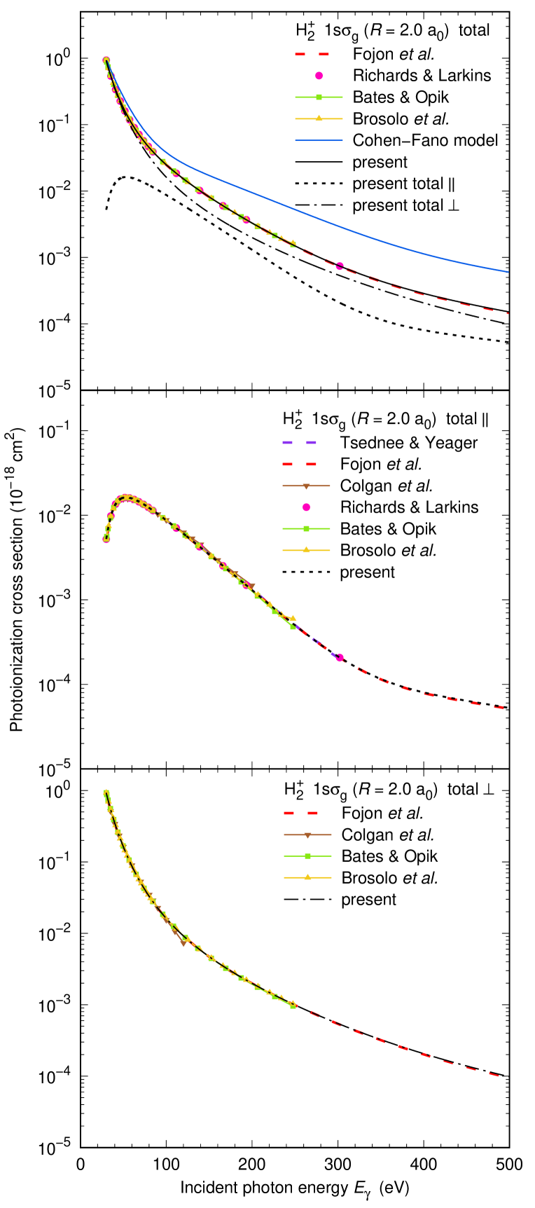
Figure 1: Total (solid black line), parallel (dotted black line), and perpendicular (dot–dashed black line) photoionization cross sections for the ground electronic state of H${}_{2}^{+}$. We compare with the results of Fojón et al. (2006), Richards & Larkins (1986), Bates & Öpik (1968), Brosolo et al. (1994), Colgan et al. (2003), Tsednee & Yeager (2018) and the Cohen & Fano (1966) model. The Cohen–Fano model cross section has been shifted and rescaled to match ours at threshold.

The perpendicular photoionization cross section is larger than the parallel photoionization cross section at all photon energies considered, the largest difference occurring near the ionization threshold. The parallel and perpendicular photoionization cross sections presented here contain contributions from the lowest five partial waves, i.e. $\lambda=1,3,5,7,9$. For the energy range considered here higher partial waves are not required as convergence is achieved by $\lambda=9$. Our cross sections are compared with those of Fojón et al. (2006), Richards & Larkins (1986), Bates & Öpik (1968), Brosolo et al. (1994), Colgan et al. (2003), and Tsednee & Yeager (2018). Excellent agreement is found in all cases. In addition, though not presented, perfect agreement is found between our cross section and those of Bates & Öpik (1968) for photoionization of the 2s$\sigma_{\mathrm{g}}$ state of H${}_{2}^{+}$.

In Figure 1 we also compare our total photoionization cross section with the model, Equation (2), proposed by Cohen & Fano (1966). The ground state photoionization cross section for He⁺ was used as the atomic cross section in the Cohen–Fano model. After shifting the model photoionization cross section to the correct threshold and rescaling it to match our photoionization cross section at the ionization threshold, we find that the Cohen–Fano model cross section has similar qualitative behavior at low energies but at high energies it does not decay as quickly as our photoionization cross section. This leads to significant differences in magnitude at higher incident photon energies, which is in agreement with the observations of Fojón et al. (2006). The Cohen–Fano model makes three assumptions: (i) ionization is effectively a one–electron process, (ii) the initial state wave function is well described within the Linear Combination of Atomic Orbitals approximation, and (iii) the ionized electron is well described by a plane wave or single–center spherical wave. In the case of H${}_{2}^{+}$ the first of these assumptions is valid, the validity of the second assumption depends on the size of the basis of atomic orbitals, and the third assumption is not satisfied. Hence, it is not surprising that our photoionzation cross section differs from the Cohen–Fano model photoionization cross section.

3.2 Vibrationally–Resolved Photoionization

Total, parallel, and perpendicular photoionization cross sections for all bound vibrational levels of the 1s$\sigma_{\mathrm{g}}$ state are shown in Figure 2. The total photoionization cross sections are typically dominated by perpendicular contributions. For $v\geq 4$, the cross sections near their respective thresholds increase significantly in magnitude as the vibrational level $v$ increases. The increase in the magnitude of the cross section as $v$ increases is also observed in electron scattering and photodissociation of H${}_{2}^{+}$ (Zammit et al., 2014; Scarlett et al., 2017; Zammit et al., 2017), and electron scattering from H₂ (Scarlett et al., 2021a). However, for $v\leq 3$ the near threshold cross section decreases as $v$ increases. This behaviour in the total cross section follows from the perpendicular photoionization cross sections. Oscillations in the cross sections just above the ionization threshold can also be seen. We believe these oscillations are physical as the only approximation used in these calculations is the Born–Oppenheimer approximation. Similar behaviour is also observed in electron scattering cross sections (Scarlett et al., 2021a). The ionization thresholds also shifts to lower energies as the initial vibrational level increases.

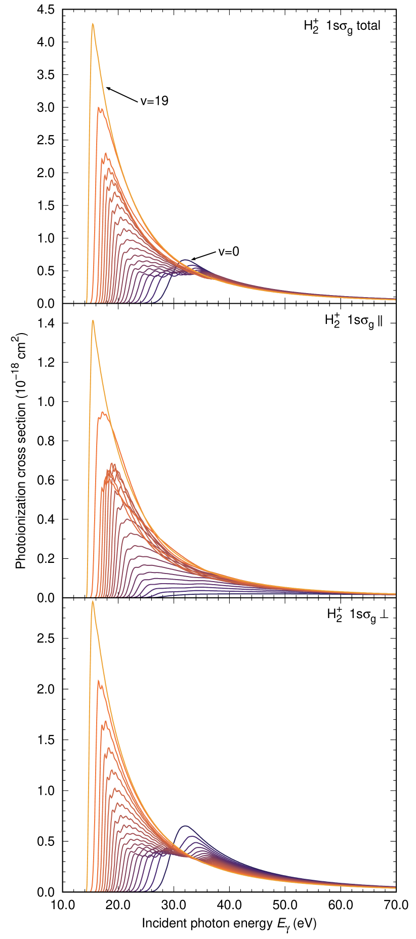
Figure 2: Total, parallel, and perpendicular photoionization cross sections for all bound vibrational levels of the 1s$\sigma_{\mathrm{g}}$ state of H${}_{2}^{+}$.

The origin of the oscillations present in the near threshold cross sections for photoionization from excited vibrational levels is investigated further in appendix C.

3.3 Isotopologue Effects

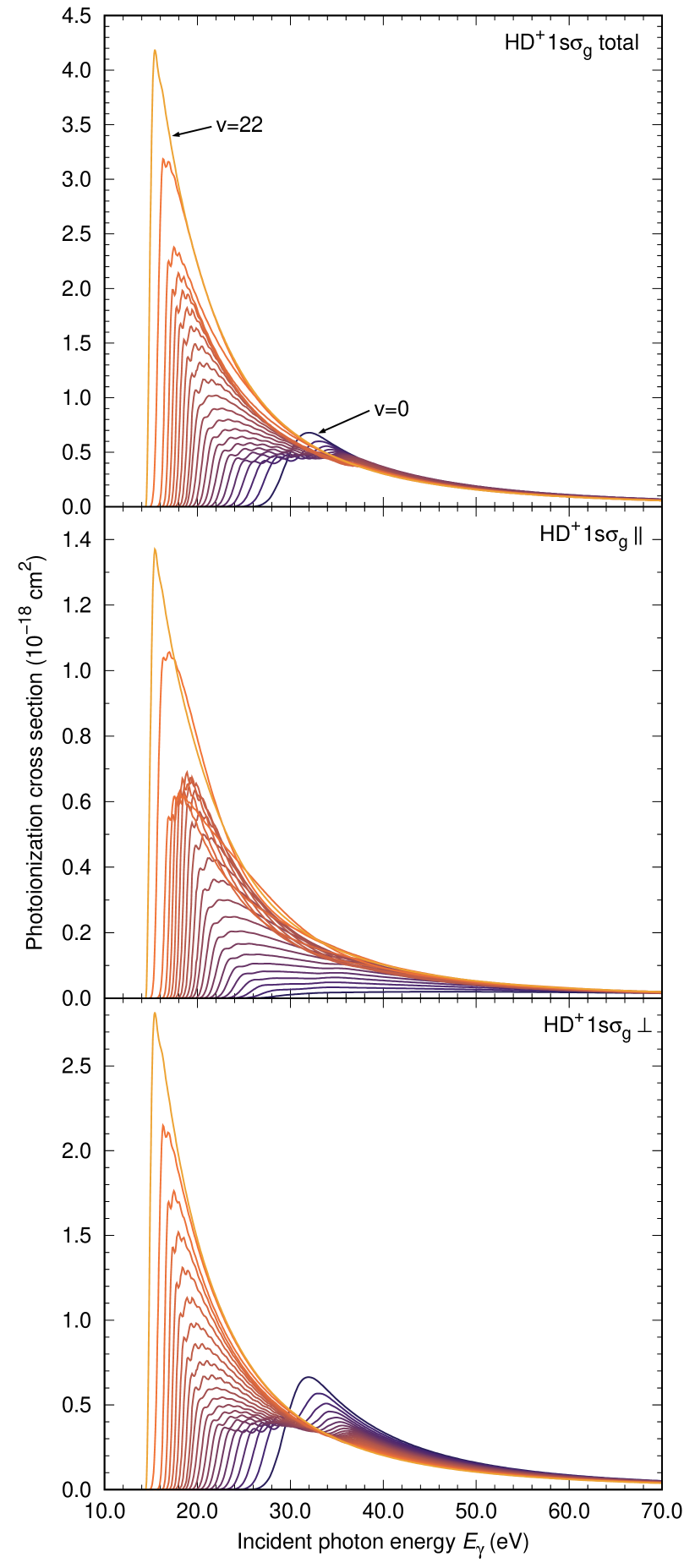
Figure 3: Same as Figure 2 but for HD⁺.

Figure 4: Same as Figure 2 but for D${}_{2}^{+}$.

In Figures 3 and 4 we present photoionization cross sections for all bound vibrational levels of the ground electronic state of HD⁺, and D${}_{2}^{+}$ respectively. These cross section exhibit the same behavior as the H${}_{2}^{+}$ cross sections, i.e. the cross section increasing in magnitude near the ionization threshold with increasing vibrational level and oscillations in the cross sections occurring near the ionization threshold for photoionization from excited vibrational levels.

The cross sections for photoionization from the ground vibrational level of H${}_{2}^{+}$ and its deuterated isotopologues are compared in Figure 5. There are only minor differences between the cross sections for each isotopologue, with the maximum value of the cross section increasing slightly and the ionization threshold shifting to a higher energy as the nuclear reduced mass of the isotopologue increases. This is due to the energy of the ground vibrational level decreasing as the nuclear reduced mass increases, which results in the ionization threshold shifting to a higher energy. The increase in the maximum value of the photoionization cross section for heavier isotoplogues is a result of the vibrational wave function being more densely concentrated in the region where the electronic part of the photoionization cross section is larger. At higher incident photon energies the photoionization cross sections for the different isotopologues are identical.

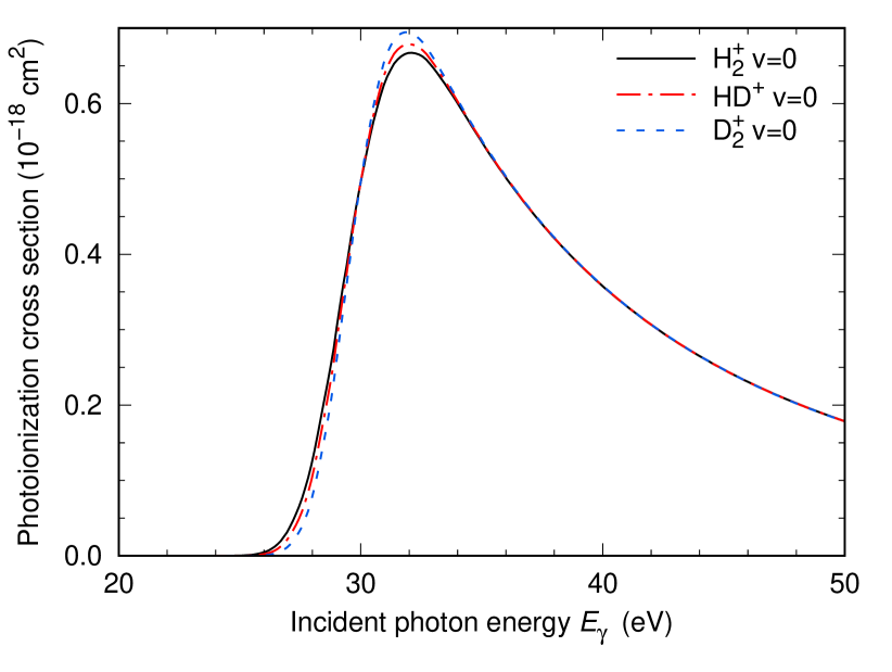
Figure 5: Total photoionization cross sections for the ground state of H${}_{2}^{+}$ and its deuterated isotopologues.

In Figure 6, LTE photoionization cross sections for H${}_{2}^{+}$ and its deuterated isotopologues are presented over a range of gas temperatures. These cross sections can be integrated with arbitrary spectral energy density distributions to obtain photoionization rate coefficients.

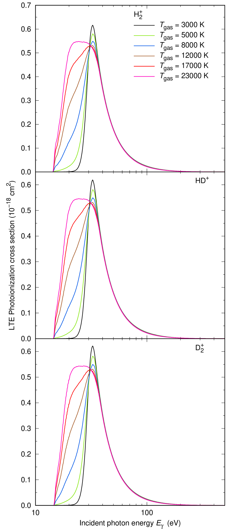
Figure 6: LTE photoionization cross sections for H${}_{2}^{+}$ and its deuterated isotopologues at gas temperatures of $3\,000$, $5\,000$, $8\,000$, $12\,000$, $17\,000$, and $23\,000$ K.

3.4 Photoionization Rate Coefficients

Vibrationally–resolved and LTE photoionization rate coefficients are given Figures 7–9, with analytic fits included for the LTE rate coefficients. As discussed in Section 3.3, there are practically no isotopologue effects present in the photoionization cross sections which results in the LTE photoionization rate coefficients for each isotopologue being very similar.

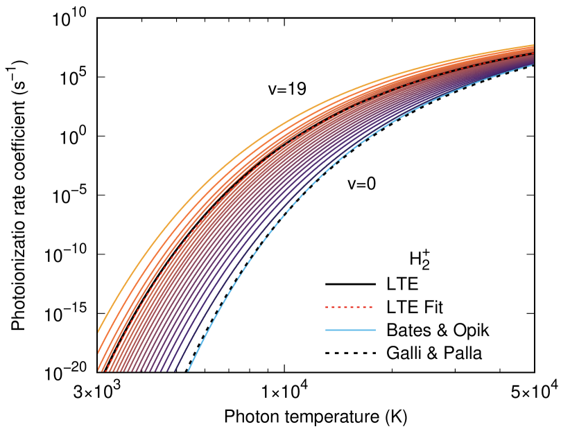
Figure 7: Vibrationally–resolved and LTE photoionization rate coefficients for H${}_{2}^{+}$ as a function of radiation temperature. The analytic fit of Galli & Palla (1998) and the rate coefficient we have calculated using the cross sections of Bates & Öpik (1968) are presented for comparison. The analytic fit function in Equation (12) is presented for the LTE photoionization rate coefficients.

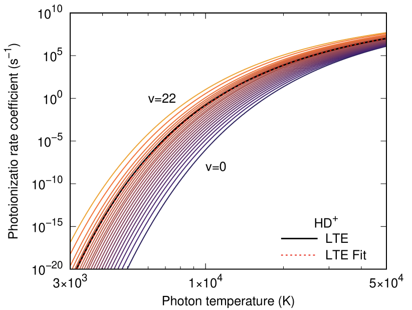
Figure 8: Same as Figure 7 but for HD⁺.

Figure 9: Same as Figure 7 but for D${}_{2}^{+}$.

The analytic model given by Galli & Palla (1998) was determined by fitting to a photoionization rate coefficient calculated using the fixed–nuclei cross sections of Bates & Öpik (1968). In Figure 7 we verify our rate coefficients by calculating a photoionzation rate coefficient using the results of Bates & Öpik (1968) and confirming that it agrees with the analytic fit of Galli & Palla (1998). The cross sections of Bates & Öpik (1968) are calculated within the fixed–nuclei approximation, which would approximate the $v=0$ photoionization cross section. Hence, photoionization rate coefficients calculated using the Bates & Öpik (1968) cross sections are similar to our $v=0$ rate coefficients with the difference being smallest at higher temperatures. Photoionization rate coefficients for excited vibrational levels, in Figure 7, are much larger than the rate coefficient for the ground vibrational level. This results in the LTE photoionization rate coefficient being several orders of magnitude larger than the currently used values of Galli & Palla (1998). The significant variance in the magnitude of the vibrationally–resolved rate coefficients is due to the ionization threshold for excited vibrational levels shifting to lower photon energies as seen in Figure 10. This leads to a larger overlap between the cross section and the spectral energy density distribution, Equation (8), resulting in a larger photoionization rate coefficient.

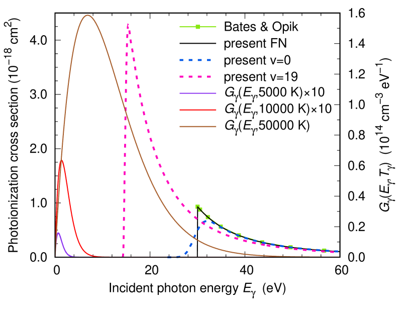
Figure 10: Present fixed–nuclei $R=2~{}a_{0}$, and vibrationally–resolved $v=0$ and $v=19$ photoionization cross sections superimposed with the spectral energy density distribution given by Equation (8). The fixed–nuclei photoionization cross sections of Bates & Öpik (1968) are presented for comparison. The spectral energy density distributions at $5\,000$ K and $10\,000$ K have been scaled by a factor of 10 for clarity.

We use the analytic fit function of Galli & Palla (1998),

$$\mathcal{R}^{(\mathrm{PI})}_{n_{i}v_{i}}(T_{\gamma})=A\,T_{\gamma}^{B}\,\mathrm{e}^{C/T_{\gamma}}$$ (12)

and determine fitting parameters $A$, $B$, and $C$ for the vibrationally–resolved and LTE photoionization rate coefficients for H${}_{2}^{+}$ and its deuterated isotopologues. Fitting parameters for the LTE photoionization rate coefficient for H${}_{2}^{+}$, HD⁺, and D${}_{2}^{+}$ are presented in Table 2, and were determined using standard non–linear least–squares curving fitting. Fitting parameters for the vibrationally–resolved rate coefficients are available on Zenodo under an open-source Creative Commons Attribution license: https://doi.org/10.5281/zenodo.8304060 (catalog doi:10.5281/zenodo.8304060).

Table 2: Fitting parameters in Equation 12 for the LTE photoionization rate coefficient for H${}_{2}^{+}$ and its deuterated isotopologues.

isotopologue	A (s-1 K-B)		B	C (K)
H${}_{2}^{+}$	113.13	1.42	-196236
HD+	134.22	1.41	-197978
D${}_{2}^{+}$	150.67	1.40	-199736

4 Conclusion

We have calculated cross sections and rate coefficients for photoionization from all bound vibrational states of H${}_{2}^{+}$, HD⁺, and D${}_{2}^{+}$ and presented a benchmark set of H${}_{2}^{+}$ fixed–nuclei photoionization cross sections. Vibrationally–resolved and LTE photoionization rate coefficients are calculated for H${}_{2}^{+}$ and its deuterated isotopologues. The present vibrationally–resolved photoionization rate coefficients are found to be several orders of magnitudes larger than the currently accepted values in the literature. Fitting parameters for an analytic model of the vibrationally–resolved and LTE photoionization rate coefficients have been provided for modeling the effects of photoionization of H${}_{2}^{+}$ and its isotopologues in astrophysical plasmas.

Our benchmark results are found to be in excellent agreement with available theoretical results in all cases. It was found that the Cohen–Fano model photoionization cross section can describe the overall shape of the H${}_{2}^{+}$ photoionization cross section, but does not reproduce the correct magnitude. Near threshold cross sections for photoionization from vibrationally excited levels of H${}_{2}^{+}$ and its isotopologues were found to contain oscillations. These oscillations were shown to be due to nodes in the vibrational wave functions. The magnitude of the vibrationally–resolved photoionization cross sections increases as the initial vibrational level increases, while the ionization threshold shifts to lower energies. No significant isotopologue effects were found in the cross sections. Data files for our set of benchmark cross sections, rate coefficients, and fitting parameters for H${}_{2}^{+}$, HD⁺, and D${}_{2}^{+}$ are available on Zenodo under an open-source Creative Commons Attribution license: https://doi.org/10.5281/zenodo.8304060 (catalog doi:10.5281/zenodo.8304060). Using the data supplied with this manuscript the reader can construct thermally–averaged photoionization cross sections, which can then be integrated with an arbitrary spectral energy density distribution to obtain photoionization rate coefficients.

Appendix A Molecular Target Structure

We start by applying the Born–Oppenheimer approximation which assumes that the electronic and nuclear parts of the target wave function are separable, Equation (3). The unseparated electronic Hamiltonian of H${}_{2}^{+}$ and its isotopologues in prolate spheroidal coordinates is given by

$$H=\frac{-1/2}{\left(\rho+\tfrac{R}{2}\right)^{2}-\left(\tfrac{R}{2}\eta\right)^{2}}\left\{\frac{\partial}{\partial\rho}\left[\rho(\rho+R)\frac{\partial}{\partial\rho}\right]+\frac{\partial}{\partial\eta}\left[(1-\eta^{2})\frac{\partial}{\partial\eta}\right]+\left[\frac{R^{2}/4}{\rho(\rho+R)}+\frac{1}{1-\eta^{2}}\right]\frac{\partial^{2}}{\partial\phi^{2}}+2(2\rho+R)\right\},$$ (A1)

where the quasi–radial and quasi–angular coordinates are

$$\qquad\rho=\frac{r_{1}+r_{1}}{2}-\frac{R}{2},\qquad\qquad\eta=\frac{r_{1}-r_{2}}{R}.$$ (A2)

Here $r_{1}$ and $r_{2}$ are the coordinates of the electron relative to the two nuclei, $R$ is the internuclear separation, $\phi$ is the usual azimuthal coordinate. Bound electronic states are obtained by diagonalizing the unseparated electronic Hamiltonian, Equation (A1), in a Sturmian basis $\{\varphi_{k\ell m}\}$, and are represented by

$$\psi_{n}^{m}(\rho,\eta,\phi;R)=\sum_{k=1}^{k_{\mathrm{max}}}\sum_{\ell=\left|m\right|}^{\ell_{\mathrm{max}}}C^{(n)}_{k\ell}\varphi_{k\ell m}(\rho,\eta,\phi),$$ (A3)

where

$$\varphi_{k\ell m}(\rho,\eta,\phi)=f_{k}^{m}(\rho)Y_{\ell}^{m}(\eta,\phi),$$ (A4)

$$f_{k}^{m}(\rho)=\sqrt{2\alpha_{m}\frac{(k-1)!}{(k+m-1)!}}(2\alpha_{m}\rho)^{m/2}\mathrm{e}^{-\alpha_{m}\rho}L_{k-1}^{m}(2\alpha_{m}\rho).$$ (A5)

Here, $L_{k-1}^{m}$ are the associated Laguerre polynomials, $Y_{\ell}^{m}$ are spherical harmonics, $\alpha_{m}$ is an exponential fall–off parameter, and $k$ is an index. These basis functions are orthogonal with respect to their coordinates:

$$\int_{0}^{\infty}\mathrm{d}\rho\,f_{k^{\prime}}^{m}(\rho)f_{k}^{m}(\rho)=\delta_{k^{\prime}k},$$ (A6)

$$\int_{0}^{2\pi}\!\mathrm{d}\phi\int_{-1}^{1}\!\mathrm{d}\eta\,Y_{\ell^{\prime}}^{m^{\prime}*}(\eta,\phi)Y_{\ell}^{m}(\eta,\phi)=\delta_{\ell^{\prime}\ell}\delta_{m^{\prime}m},$$ (A7)

but not the volume element in prolate spheroidal coordinates. The overlap between the basis functions, Equation (A4), with the volume element

$$\mathrm{d}V=\left[\left(\rho+\tfrac{R}{2}\right)^{2}-\left(\tfrac{R}{2}\eta\right)^{2}\right]\mathrm{d}\rho\mathrm{d}\eta\mathrm{d}\phi,$$ (A8)

is given by (Savage, 2018)

$$\braket{k^{\prime}\ell^{\prime}m^{\prime}}{k\ell m} =\int\mathrm{d}V\,\varphi^{*}_{k^{\prime}\ell^{\prime}m^{\prime}}(\rho,\eta,\phi)\varphi_{k\ell m}(\rho,\eta,\phi)$$

$$=\delta_{\ell^{\prime}\ell}\delta_{m^{\prime}m}b_{k^{\prime}k}^{m}-\delta_{k^{\prime}k}\tfrac{R^{2}}{6}C_{\ell^{\prime}020}^{\ell 0}C_{\ell m20}^{\ell^{\prime}m^{\prime}},$$ (A9)

where

$$b_{k^{\prime}k}^{m}=\begin{cases}(2\alpha_{m})^{-2}\sqrt{k(k+m)(k+1)(k+m+1)}&k^{\prime}=k+2,\\ -(2\alpha_{m})^{-2}\sqrt{k(k+m)}(4k+2m+2\alpha_{m}R)&k^{\prime}=k+1,\\ (2\alpha_{m})^{-2}(6k^{2}-6k+6km-3m+m^{2}+2)+\tfrac{2k-1+m}{2\alpha_{m}}+\tfrac{R^{2}}{6}&k^{\prime}=k,\\ -(2\alpha_{m})^{-2}\sqrt{(k-1)(k-1+m)}(4k-4+2m+2\alpha_{m}R)&k^{\prime}=k-1,\\ (2\alpha_{m})^{-2}\sqrt{(k-1)(k-1+m)(k-2)(k-2+m)}&k^{\prime}=k-2,\\ 0&$otherwise$,\end{cases}$$ (A10)

and $C_{\ell m\ell^{\prime}m^{\prime}}^{LM}$ is a Clebsh–Gordon Coefficient. The expansion coefficients, $C^{(n)}_{k\ell}$ in Equation (A3), and the bound state energy levels, $E$, are obtained by solving the generalized eigenvalue problem

$$\boldsymbol{H}\boldsymbol{C}=E\boldsymbol{B}\boldsymbol{C}.$$ (A11)

Here $\boldsymbol{H}$ is the Hamiltonian matrix with matrix elements given by

$$\braket{k^{\prime}\ell^{\prime}m^{\prime}}{H}{k\ell m}=\delta_{\ell^{\prime}\ell}\delta_{m^{\prime}m}\Bigg{[}h_{k^{\prime}k}^{\ell m}-\frac{m^{2}R}{8}\int_{0}^{\infty}\!\mathrm{d}\rho\,\frac{f_{k^{\prime}}^{m}(\rho)f_{k}^{m}(\rho)}{\rho+R}\Bigg{]},$$ (A12)

where

$$h_{k^{\prime}k}^{\ell m}=\begin{cases}-\tfrac{1}{8}\sqrt{k(k+m)(k+1)(k+1+m)}&k^{\prime}=k+2,\\ \tfrac{1}{4}\sqrt{k(k+m)}\left(\alpha_{m}R-\tfrac{4}{\alpha_{m}}\right)&k^{\prime}=k+1,\\ \tfrac{1}{4}\bigg{[}k^{2}-k+km-\tfrac{m}{2}+1+4R+2\ell(\ell+1)+(2k-1+m)\left(\alpha_{m}R+\tfrac{4}{\alpha_{m}}\right)\bigg{]}&k^{\prime}=k,\\ \tfrac{1}{4}\sqrt{(k-1)(k-1+m)}\left(\alpha_{m}R-\tfrac{4}{\alpha_{m}}\right)&k^{\prime}=k-1,\\ -\tfrac{1}{8}\sqrt{(k-1)(k-1+m)(k-2)(k-2+m)}&k^{\prime}=k-2,\\ 0&$otherwise$,\end{cases}$$ (A13)

and $\boldsymbol{B}$ is the overlap matrix with elements given by Equation (A), and $\boldsymbol{C}$ contains the expansion coefficients as its columns.

Electronic continuum states are calculated using the approach of Singor et al. (2022). The non–relativistic electronic Schrödinger equation for the molecular hydrogen ion is separable into quasi–radial and quasi–angular parts in prolate spheroidal coordinates and is given by

$$\Bigg{\{}\frac{\mathrm{d}}{\mathrm{d}\rho}\left[\rho(\rho+R)\frac{\mathrm{d}}{\mathrm{d}\rho}\right]-\frac{m^{2}R^{2}}{4\rho(\rho+R)}+2(2\rho+R)+2E\rho(\rho+R)-A_{\lambda}^{\left|m\right|}(E,R)\Bigg{\}}\Xi_{\lambda}^{\left|m\right|}(\rho;R) =0,$$ (A14)

$$\Bigg{\{}\frac{\mathrm{d}}{\mathrm{d}\eta}\left[(1-\eta^{2})\frac{\mathrm{d}}{\mathrm{d}\eta}\right]-\frac{m^{2}}{1-\eta^{2}}+\tfrac{1}{2}ER^{2}(1-\eta^{2})+A_{\lambda}^{\left|m\right|}(E,R)\Bigg{\}}\Upsilon_{\lambda}^{m}(\eta,\phi;R) =0,$$ (A15)

where $E$ is the energy eigenvalue, $A_{\lambda}^{\left|m\right|}(E,R)$ is the separation constant, $m$ is the projection of the orbital angular momentum onto the internuclear axis, and $\lambda$ is a pseudo–angular momentum used to label states. The pseudo–angular momentum $\lambda$ is related to the number of zeros $q$, of $\Upsilon_{\lambda}^{m}(\eta,\phi;R)$ in the interval $\eta\in(-1,1)$ by $\lambda=q+\left|m\right|$ and corresponds to the orbital angular momentum in the combined nuclei limit, i.e. $\lambda\to\ell$ as $R\to 0$. The quasi–angular wave functions are obtained by expanding the spheroidal harmonics in Equation (A15) as a series of spherical harmonics of the same $m$. The solution to the quasi–radial equation, Equation (A14), is started using a power series expansion and then propagated using an Adams–Moulton predictor–corrector algorithm. An asymptotic series is then used to normalize the wave function. The electronic continuum states of a H${}_{2}^{+}$ isotopologue can then be written as

$$\psi_{E\lambda}^{m}(\rho,\eta,\phi;R) =\Xi_{\lambda}^{\left|m\right|}(\rho;R)\Upsilon_{\lambda}^{m}(\eta,\phi;R),$$ (A16)

$$=\Xi_{\lambda}^{\left|m\right|}(\rho;R)\sum_{\ell=\left|m\right|}^{\ell_{\mathrm{max}}}\mathcal{C}_{\ell m}^{\lambda}(R)\,Y_{\ell}^{m}(\eta,\phi).$$ (A17)

The non–relativistic Born–Oppenheimer Schrödinger equation for the vibrational wave functions is

$$\left[-\frac{1}{2\mu}\frac{\mathrm{d}^{2}}{\mathrm{d}R^{2}}+\epsilon_{n}(R)-\varepsilon_{nv}\right]\nu_{nv}(R)=0,$$ (A18)

where $n$ specifies the electronic state, $\epsilon_{n}(R)$ is the potential energy curve for the electronic state $n$, $\mu$ is the nuclear reduced mass of the H${}_{2}^{+}$ isotopologue, and the centrifugal term is neglected in the current non–rotationally resolved calculations. Within the Born–Oppenheimer approximation the only difference between the isotopologues is the value of $\mu$. The values of the nuclear reduced mass for H${}_{2}^{+}$, HD⁺, and D${}_{2}^{+}$ are given in Table 3, along with the number of bound vibrational levels. Bound vibrational wave functions are found by expanding $\nu_{nv}(R)$ as

$$\nu_{nv}(R)=\sum_{k=1}^{k_{\mathrm{max}}}\tilde{C}_{knv}\,\phi_{k}(R),$$ (A19)

where

$$\phi_{k}(R)=\frac{\sqrt{\tilde{\alpha}}}{k}\,2\tilde{\alpha}R\,\mathrm{e}^{-\tilde{\alpha}R}\,L^{1}_{k-1}(2\tilde{\alpha}R).$$ (A20)

Here $\tilde{\alpha}$ is an exponential fall–off parameter, and $L^{1}_{k-1}$ are the associated Laguerre polynomials. The expansion coefficients $\tilde{C}_{knv}$ in Equation (A19) are obtained by diagonalizing the vibrational Hamiltonian in the basis $\{\phi_{k}\}$.

Table 3: Nuclear reduced masses in atomic units, and number of bound vibrational levels in the ground electronic state for H${}_{2}^{+}$ and its deuterated isotopologues, where $m_{\mathrm{e}}$ is the electron mass.

isotopologue	$\mu$ ($m_{\mathrm{e}}$)		number of bound
		vibrational levels
H${}_{2}^{+}$	918.076351	20
HD+	1223.899246	23
D${}_{2}^{+}$	1835.241507	28

Appendix B Dipole Matrix Elements

Matrix elements of the dipole operator can be given in the length $(\mathsf{L})$ or velocity $(\mathsf{V})$ gauge,

$$\braket{\psi_{E\lambda}^{m^{\prime}}}{d_{\kappa}}{\psi_{n}^{m}}=\braket{\psi_{E\lambda}^{m^{\prime}}}{\mathsf{L}_{\kappa}}{\psi_{n}^{m}}=\frac{\braket{\psi_{E\lambda}^{m^{\prime}}}{\mathsf{V}_{\kappa}}{\psi_{n}^{m}}}{E_{n}-E}.$$ (B1)

The length gauge dipole operator is

$$\mathsf{L}_{\kappa} =\mathcal{L}_{\kappa}(\rho)\sqrt{\tfrac{4\pi}{3}}\,Y_{1}^{\kappa}(\eta,\phi),$$ (B2)

$$\mathcal{L}_{\kappa}(\rho) =\begin{cases}\rho+\tfrac{R}{2}&\kappa=0,\\ \sqrt{\rho(\rho+R)}&\kappa=\pm 1,\end{cases}$$ (B3)

and the velocity gauge dipole operator is

$$\mathsf{V}_{\kappa} =\begin{cases}\dfrac{1}{\rho(\rho+R)+\frac{R^{2}}{4}(1-\eta^{2})}\left[\rho(\rho+R)\eta\dfrac{\partial}{\partial\rho}+(1-\eta^{2})\left(\rho+\frac{R}{2}\right)\dfrac{\partial}{\partial\eta}\right]&\kappa=0,\\[10.0pt] \dfrac{\mp\mathrm{e}^{\pm\mathrm{i}\phi}}{\sqrt{2}}\dfrac{\sqrt{\rho(\rho+R)}}{\rho(\rho+R)+\frac{R^{2}}{4}(1-\eta^{2})}\left[\sqrt{1-\eta^{2}}\left(\rho+\frac{R}{2}\right)\dfrac{\partial}{\partial\rho}\pm\mathrm{i}\dfrac{R^{2}}{4}\dfrac{\sqrt{1-\eta^{2}}}{\rho(\rho+R)}\dfrac{\partial}{\partial\phi}\right.\\ \hskip 140.0pt-\left.\left(\eta\sqrt{1-\eta^{2}}\dfrac{\partial}{\partial\eta}\mp\dfrac{\mathrm{i}}{\sqrt{1-\eta^{2}}}\dfrac{\partial}{\partial\phi}\right)\right]&\kappa=\pm 1.\end{cases}$$ (B4)

The components of the electronic length gauge dipole matrix elements are given by (Zammit et al., 2017)

$$\braket{\psi_{E\lambda}^{m^{\prime}}}{\mathsf{L}_{\kappa}}{\psi_{n}^{m}}=\sum_{\ell^{\prime}}\sum_{k\ell}\mathcal{C}_{\ell^{\prime}m^{\prime}}^{\lambda}C^{(n)}_{k\ell}\int_{0}^{\infty}\mathrm{d}\rho\,\,\Xi_{\lambda}^{\left|m^{\prime}\right|}(\rho)\,\mathcal{L}_{\kappa}(\rho)f_{k}^{m}(\rho)J_{1,\kappa}^{(\ell^{\prime}m^{\prime},\ell m)}(\rho),$$ (B5)

where $C_{k\ell m}$ are the expansion coefficients in Equation (A3) and $J_{1,\kappa}^{\ell^{\prime}m^{\prime},\ell m}(\rho)$ is the angular integral with the volume element,

$$J_{L,M}^{(\ell^{\prime}m^{\prime},\ell m)}(\rho)= \int_{0}^{2\pi}\int_{-1}^{1}\mathrm{d}\eta\mathrm{d}\phi\,Y_{\ell^{\prime}}^{m^{\prime}*}(\eta,\phi)\sqrt{\tfrac{4\pi}{2L+1}}Y_{L}^{M}(\eta,\phi)Y_{\ell}^{m}(\eta,\phi)\left[\rho(\rho+R)+\tfrac{R^{2}}{4}(1-\eta^{2})\right].$$ (B6)

The angular integral can be evaluated analytically

$$J_{1,0}^{(\ell^{\prime}m^{\prime},\ell m)}(\rho)= \left[\rho(\rho+R)+\tfrac{R^{2}}{10}\right]A_{m^{\prime}}^{\ell^{\prime}}{}_{0}^{1}{}_{m}^{\ell}-\tfrac{R^{2}}{10}A_{m^{\prime}}^{\ell^{\prime}}{}_{0}^{3}{}_{m}^{\ell},$$ (B7)

$$J_{1,\pm 1}^{(\ell^{\prime}m^{\prime},\ell m)}(\rho)= \left[\rho(\rho+R)+\tfrac{R^{2}}{5}\right]A_{m^{\prime}}^{\ell^{\prime}}{}_{\pm 1}^{1}{}_{m}^{\ell}-\tfrac{R^{2}}{5\sqrt{6}}A_{m^{\prime}}^{\ell^{\prime}}{}_{\pm 1}^{3}{}_{m}^{\ell},$$ (B8)

where

$$A_{m_{1}}^{\ell_{1}}{}_{m_{2}}^{\ell_{2}}{}_{m_{3}}^{\ell_{3}} =\int_{0}^{2\pi}\int_{-1}^{1}\!\mathrm{d}\eta\mathrm{d}\phi\,Y_{\ell_{1}}^{m_{1}*}(\eta,\phi)\sqrt{\tfrac{4\pi}{2\ell_{2}+1}}Y_{\ell_{2}}^{m_{2}}(\eta,\phi)Y_{\ell_{3}}^{m_{3}}(\eta,\phi)$$

$$=(-1)^{\ell_{2}}\,C_{\ell_{1}0\ell_{2}0}^{\ell_{3}0}\,C_{\ell_{3}m_{3}\ell_{2}m_{2}}^{\ell_{1}m_{1}}.$$ (B9)

In the velocity gauge the components of the electronic dipole operator are

$$\braket{\psi_{E\lambda}^{m^{\prime}}}{\mathsf{V}_{0}}{\psi_{n}^{m}} =\sum_{\ell^{\prime}}\sum_{k\ell}\mathcal{C}_{\ell^{\prime}m^{\prime}}^{\lambda}C^{(n)}_{k\ell}\,A_{m^{\prime}}^{\ell^{\prime}}{}_{0}^{1}{}_{m}^{\ell}\int_{0}^{\infty}\!\mathrm{d}\rho\,\,\Xi_{\lambda}^{\left|m^{\prime}\right|}(\rho)\!\left[\rho(\rho+R)\frac{\partial}{\partial\rho}+y_{\ell^{\prime}\ell}\left(\rho+\tfrac{R}{2}\right)\right]f_{k}^{m}(\rho),$$ (B10)

$$\braket{\psi_{E\lambda}^{m^{\prime}}}{\mathsf{V}_{\pm 1}}{\psi_{n}^{m}} =-\sum_{\ell^{\prime}}\sum_{k\ell}\mathcal{C}_{\ell^{\prime}m^{\prime}}^{\lambda}C^{(n)}_{k\ell}\,A_{m^{\prime}}^{\ell^{\prime}}{}_{\pm 1}^{1}{}_{m}^{\ell}\int_{0}^{\infty}\!\mathrm{d}\rho\,\,\Xi_{\lambda}^{\left|m^{\prime}\right|}(\rho)\sqrt{\rho(\rho+R)}\left[\left(\rho+\tfrac{R}{2}\right)\!\frac{\partial}{\partial\rho}+\frac{\left|m\right|R^{2}}{4\rho(\rho+R)}+y_{\ell^{\prime}\ell}\right]f_{k}^{m}(\rho),$$ (B11)

where

$$y_{\ell^{\prime}\ell} =\begin{cases}-\ell&\ell^{\prime}=\ell+1,\\ \ell+1&\ell^{\prime}=\ell-1.\end{cases}$$ (B12)

Appendix C Origin of the Oscillations in the Vibrationally Resolved Cross Sections

In Figure 11 the origin of these oscillations is investigated. The top panel of Figure 11 shows the $v=1$ photoionization cross section in the region of the oscillations, while the bottom panel shows the components of the integrand in Equation (5) used to calculate the cross section in the top panel. It can be seen that the overlap of the squared $v=1$ vibrational wave function with the electronic part of the photoionization cross section, Equation (6), increases as the incident photon energy increases until a node in the vibrational wave function is reached. When a node is reached the overall overlap between the wave function squared and the cross section decreases. Therefore the near threshold oscillations in the photoionization cross sections for vibrationally excited states is due to nodes in the excited vibrational wave functions.

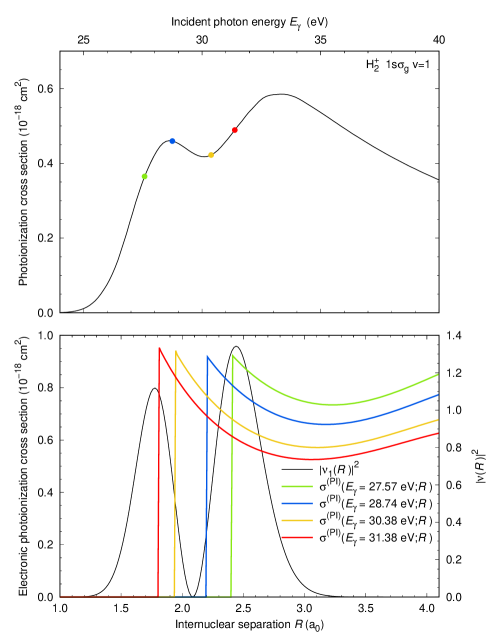
Figure 11: (Top) The near threshold $v=1$ photoionization cross section as a function of incident photon energy. (Bottom) Norm squared of the $v=1$ vibrational wave function and the electronic part of the photoionization cross section, Equation (6), as a function of internuclear separation $R$. The first non–zero point of the electronic part of the photoionisation cross section shifts to a lower value of $R$ as the incident photon energy increases. The corresponding points in the top panel are indicated with dots of the same color.

The shift of the ionization threshold to lower energies as $v$ increases can also be explained by the by the overlap between the electronic part of the photoionization cross section and the norm squared of the vibrational wave function. The vibrational wave function extends to larger internuclear separations as the vibrational level increases. It can been seen in Figure 11 at lower incident photon energies the first non–zero point of the electronic part of the photoionization cross section occurs at a larger internuclear separation. Therefore, higher vibrational levels have wave functions that overlap with the electronic part of the photoionization cross section at lower incident photon energies, this results in the shift of the ionization threshold to lower energies.

References

- Aleman & Gruenwald (2004) Aleman, I., & Gruenwald, R. 2004, The Astrophysical Journal, 607, 865
- Arkhipov et al. (2018) Arkhipov, D., Astashkevich, S., Mityureva, A., & Smirnov, V. 2018, Physics Letters A, 382, 1881
- Bates & Öpik (1968) Bates, D. R., & Öpik, U. 1968, Journal of Physics B: Atomic and Molecular Physics, 1, 543
- Bates et al. (1953) Bates, D. R., Öpik, U., & Poots, G. 1953, Proceedings of the Physical Society. Section A, 66, 1113
- Brosolo & Decleva (1992) Brosolo, M., & Decleva, P. 1992, Chemical Physics, 159, 185
- Brosolo et al. (1994) Brosolo, M., Decleva, P., & Lisini, A. 1994, Chemical Physics, 181, 85
- Cohen & Fano (1966) Cohen, H. D., & Fano, U. 1966, Phys. Rev., 150, 30
- Colgan et al. (2003) Colgan, J., Pindzola, M. S., & Robicheaux, F. 2003, Phys. Rev. A, 68, 063413
- Dalgarno (1985) Dalgarno, A. 1985, Molecular Astrophysics (Dordrecht: Springer Netherlands), 3–22
- Della Picca et al. (2011) Della Picca, R., Fainstein, P. D., & Dubois, A. 2011, Phys. Rev. A, 84, 033405
- Della Picca et al. (2008) Della Picca, R., Fainstein, P. D., Martiarena, M. L., & Dubois, A. 2008, Phys. Rev. A, 77, 022702
- Della Picca et al. (2009) Della Picca, R., Fainstein, P. D., Martiarena, M. L., Sisourat, N., & Dubois, A. 2009, Phys. Rev. A, 79, 032702
- Fernández et al. (2009a) Fernández, J., Fojón, O., & Martín, F. 2009a, Phys. Rev. A, 79, 023420
- Fernández et al. (2007) Fernández, J., Fojón, O., Palacios, A., & Martín, F. 2007, Phys. Rev. Lett., 98, 043005
- Fernández et al. (2009b) Fernández, J., Yip, F. L., Rescigno, T. N., McCurdy, C. W., & Martín, F. 2009b, Phys. Rev. A, 79, 043409
- Fojón et al. (2006) Fojón, O., Palacios, A., Fernández, J., Rivarola, R., & Martín, F. 2006, Physics Letters A, 350, 371
- Ford et al. (1975) Ford, A. L., Docken, K. K., & Dalgarno, A. 1975, The Astrophysical Journal, 195, 819
- Galli & Palla (1998) Galli, D., & Palla, F. 1998, A&A, 335, 403
- Gruntman (1996) Gruntman, M. 1996, Journal of Geophysical Research: Space Physics, 101, 15555
- Haxton (2013) Haxton, D. J. 2013, Phys. Rev. A, 88, 013415
- Heays et al. (2017) Heays, A. N., Bosman, A. D., & van Dishoeck, E. F. 2017, Astronomy and Astrophysics, 602, A105
- Langhoff (1985) Langhoff, P. W. 1985, Molecular Photoionization Processes of Astrophysical and Aeronomical Interest (Dordrecht: Springer Netherlands), 551–573
- Mukherjee et al. (2006) Mukherjee, P., Fritzsche, S., & Fricke, B. 2006, Physics Letters A, 360, 287
- Richards & Larkins (1986) Richards, J. A., & Larkins, F. P. 1986, Journal of Physics B: Atomic and Molecular Physics, 19, 1945
- Savage (2018) Savage, J. S. 2018, PhD thesis, Curtin University
- Scarlett et al. (2021a) Scarlett, L. H., Fursa, D. V., Knol, J., Zammit, M. C., & Bray, I. 2021a, Phys. Rev. A, 103, L020801
- Scarlett et al. (2021b) Scarlett, L. H., Savage, J. S., Fursa, D. V., et al. 2021b, Phys. Rev. A, 103, 032802
- Scarlett et al. (2017) Scarlett, L. H., Zammit, M. C., Fursa, D. V., & Bray, I. 2017, Phys. Rev. A, 96, 022706
- Singor et al. (2022) Singor, A., Savage, J. S., Bray, I., Schneider, B. I., & Fursa, D. V. 2022, Computer Physics Communications, 108514
- Stancil (1994) Stancil, P. C. 1994, ApJ, 430, 360
- Tsednee & Yeager (2018) Tsednee, T., & Yeager, D. L. 2018, The European Physical Journal D, 72, 56
- Tseng et al. (2011) Tseng, W.-L., Johnson, R. E., Thomsen, M. F., Cassidy, T. A., & Elrod, M. K. 2011, Journal of Geophysical Research: Space Physics, 116
- Wiersma et al. (2009) Wiersma, R. P. C., Schaye, J., & Smith, B. D. 2009, Monthly Notices of the Royal Astronomical Society, 393, 99
- Zammit et al. (2014) Zammit, M. C., Fursa, D. V., & Bray, I. 2014, Phys. Rev. A, 90, 022711
- Zammit et al. (2017) Zammit, M. C., Savage, J. S., Colgan, J., et al. 2017, The Astrophysical Journal, 851, 64