Higher-order topological heat conduction on a lattice for detection of corner states

Abstract

A heat conduction equation on a lattice composed of nodes and bonds is formulated assuming the Fourier law and the energy conservation law. Based on this equation, we propose a higher-order topological heat conduction model on the breathing kagome lattice. We show that the temperature measurement at a corner node can detect the corner state which causes rapid heat conduction toward the heat bath, and that several-nodes measurement can determine the precise energy of the corner states.

I Introduction

The bulk-edge correspondence, which was originally proposed for the quantum Hall effect Hatsugai (1993a, b), plays a central role nowadays in various symmetry-protected topological (SPT) phases Kane and Mele (2005a, b); Qi et al. (2008); Hasan and Kane (2010); Qi and Zhang (2011). Recent developments have revealed the universality of the bulk-edge correspondence, including classical and/or nonequilibrium systems such as photonic crystals Raghu and Haldane (2008); Haldane and Raghu (2008); Wang et al. (2009); Ozawa et al. (2019); Kivshar (2019), phononic systems Prodan and Prodan (2009); Savin et al. (2010); Kane and Lubensky (2013); Kariyado and Hatsugai (2015); Süsstrunk and Huber (2015); Chien et al. (2018); Yoshida and Hatsugai (2019), electrical circuits Albert et al. (2015); Lee et al. (2018); Helbig et al. (2020); Yoshida et al. (2020), hydrodynamics Delplace et al. (2017); Sone and Ashida (2019), etc.

Recently, inspired by the heat conduction in anti-PT symmetric systems Li et al. (2019), heat conduction on a one-dimensional lattice which corresponds to a coarse discretization of the diffusion equation was theoretically proposed in Ref. Yoshida and Hatsugai (2021). Incorporating alternating thermal diffusivities similar to the Su-Schrieffer-Heeger (SSH) model Su et al. (1979), they showed Yoshida and Hatsugai (2021) that edge states have a significant impact on heat conduction next to the heat bath. Such an effect has been experimentally observed in Refs. Qi et al. (2022); Hu et al. (2022), indeed. It was also pointed out that the heat conduction on a lattice is reflected by the continuum diffusion equation with a similar SSH-like structure Makino et al. (2022). This implies the usefulness of the heat conduction phenomena for experimental realization of SPT phases.

On the other hand, as new types of boundary states due to topological origin, the higher-order topological insulators (HOTI) Slager et al. (2015); Hashimoto and Kimura (2016); Kunst et al. (2017); Benalcazar et al. (2017a, b); Hashimoto et al. (2017); Kunst et al. (2018); Schindler et al. (2018); Ezawa (2018) have been attracting much current interest. The boundary states called corner states, hinge states, etc., inherent in the HOTI have been observed in various systems such as electrical circuits Imhof et al. (2018), sonic crystals Zhang et al. (2019), and photonic crystals Ota et al. (2019).

In this paper, we propose a higher-order topological heat conduction system for experimental detection of corner states. We demonstrate that the corner states cause rapid heat conduction at corners next to heat bath, and temperature measurement of several nodes enables to determine the precise energy of the corner states. This is due to the localization properties of the corner states.

This paper is organized as follows. In the next section, we formulate a generic heat conduction on a lattice based on the Fourier law and the energy conservation. In Sec. III, we apply it to the heat conduction on the breathing kagome lattice, which is one of the typical models of the HOTI Ezawa (2018). In Sec. III.2.1, we show that the measurement of the temperature only at a single corner is enough to detect the corner state. We also propose more precise measurement of the energy of the corner states using several nodes around the corner in Sec. III.2.2. In Sec. III.3, the effect of the Stefan-Boltzmann thermal radiation was estimated. In the Appendix, we argue the relationship between the lattice heat equation and the continuum heat equation, using the one-dimensional model with a SSH-like structure.

II Heat conduction on a lattice

Let us consider heat conduction on lattice systems composed of nodes which are connected by bonds, as illustrated in Fig. 1.

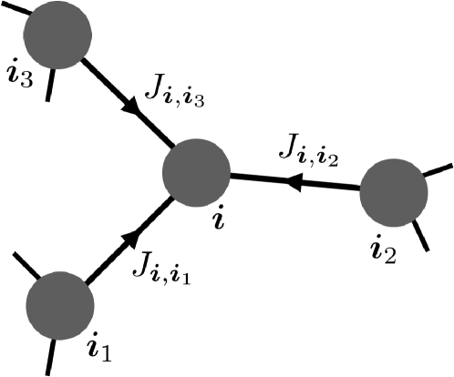
Figure 1: Nodes specified by $\bm{i}=(i_{1},i_{2})$, and bonds between them.

We assume that the node at $\bm{i}$ has volume $V_{\bm{i}}$ and surface area $S_{\bm{i}}$ characterized by the specific heat capacity $c_{\bm{i}}$ and density $\rho_{\bm{i}}$, whereas the bond between $\bm{i}$ and $\bm{i}^{\prime}$ has the area of cross section $A_{\bm{i},\bm{i}^{\prime}}$ and the length $L_{\bm{i},\bm{i}^{\prime}}$ with the thermal conductivity $k_{\bm{i},\bm{i}^{\prime}}$. We assume that the heat current flowing along the bond from $\bm{i}^{\prime}$ and $\bm{i}$ is given by the Fourier law,

$$J_{\bm{i},\bm{i}^{\prime}}=-K_{\bm{i},\bm{i}^{\prime}}(T_{\bm{i}}-T_{\bm{i}^{\prime}}),$$ (1)

where $T_{\bm{i}}$ is the temperature of nodes at $\bm{i}$ and $K_{\bm{i},\bm{i}^{\prime}}$ is the thermal conductance given, using the thermal conductivity $k_{\bm{i},\bm{i}^{\prime}}$, by

$$K_{\bm{i},\bm{i}^{\prime}}=k_{\bm{i},\bm{i}^{\prime}}\frac{A_{\bm{i},\bm{i}^{\prime}}}{L_{\bm{i},\bm{i}^{\prime}}}.$$ (2)

At each node $\bm{i}$ with the heat capacity $c_{\bm{i}}\rho_{\bm{i}}V_{\bm{i}}$, we require the continuity equation,

$$c_{\bm{i}}\rho_{\bm{i}}V_{\bm{i}}\partial_{t}T_{\bm{i}}=\sum_{n}J_{\bm{i},\bm{i}_{n}}+{\color[rgb]{0,0,0}q_{\bm{i}}},$$ (3)

where $n$ of $\bm{i}_{n}$ labels all the bonds connected with the node $\bm{i}$ (see Fig. 1), and $q_{\bm{i}}$ denotes some source term of heat. In this paper, we consider effects of the thermal radiation obeying the Stefan-Boltzmann law, ${\color[rgb]{0,0,0}q_{\bm{i}}}=\varepsilon\sigma S_{\bm{i}}(T_{0}^{4}-T_{\bm{i}}^{4})$, where $T_{0}$ is the temperature of the heat bath, $\sigma$ is the Stefan-Boltzmann constant, and $\varepsilon$ is emissivity $0\leq\varepsilon\leq 1$. Here, we assume that the thermal radiation occurs at the nodes only. Together with the Fourier law, the continuity equation can be written as

$$\partial_{t}T_{\bm{i}} =-\sum_{n}D_{{\bm{i}},{\bm{i}}_{n}}(T_{{\bm{i}}}-T_{{\bm{i}}_{n}})+\sigma_{\bm{i}}(T_{0}^{4}-T_{\bm{i}}^{4})$$

$$\equiv-\sum_{\bm{j}}{\cal H}_{\bm{i}\bm{j}}T_{\bm{j}}+\sigma_{\bm{i}}(T_{0}^{4}-T_{\bm{i}}^{4}),$$ (4)

where

$$D_{\bm{i},\bm{i}^{\prime}} \equiv\frac{k_{\bm{i},{\bm{i}}^{\prime}}}{c_{\bm{i}}\rho_{\bm{i}}}\frac{A_{\bm{i},{\bm{i}}^{\prime}}}{V_{\bm{i}}L_{\bm{i},{\bm{i}}^{\prime}}},$$

$$\sigma_{\bm{i}} \equiv\frac{\varepsilon\sigma}{c_{\bm{i}}\rho_{\bm{i}}}\frac{S_{\bm{i}}}{V_{\bm{i}}}.$$ (5)

Equation (4) with (5) is the heat conduction equation on a lattice we study in this paper. In Eq. (5), $k_{\bm{i},{\bm{i}}_{n}}/(c_{\bm{i}}\rho_{\bm{i}})$ seems the conventional thermal diffusivity. However, note that the thermal conductivity $k_{\bm{i},\bm{i}^{\prime}}$ is that of the bonds, whereas the heat capacity is $c_{\bm{i}}\rho_{\bm{i}}$ that of the nodes. Moreover, the thermal conductance $D_{\bm{i},\bm{i}^{\prime}}$ depends on the geometrical structure of the lattice system. Therefore, in the diffusion on the lattice, diffusion constants should be regarded just as effective parameters, which may be obtained by suitable renormalization from the continuum heat conduction equation. We exemplify this fact in the Appendix, comparing the heat equation in one dimension discretized by fine meshes and coarse meshes.

As an experimental implementation, we assume that initially all nodes have the same temperature as the heat bath $T_{0}$, and that at time $t=0$, some nodes are heated up to $T_{0}+\delta T$, which causes the heat conduction on a lattice. In such an experiment, it may be convenient to introduce the notation

$$T_{\bm{i}}=\delta T(\phi_{\bm{i}}+\phi_{0}),\quad(0\leq\phi_{\bm{i}}\leq 1),$$ (6)

where $\phi_{0}=T_{0}/\delta T$. Then Eq. (4) can be written as

$$\partial_{t}\phi_{\bm{i}} =-\sum_{\bm{j}}{\cal H}_{\bm{i}\bm{j}}\phi_{\bm{j}}+\alpha_{\bm{i}}\left[\phi_{0}^{4}-(\phi_{\bm{i}}+\phi_{0})^{4}\right],$$ (7)

where

$$\alpha_{\bm{i}}=\sigma_{\bm{i}}\delta T^{3}.$$ (8)

In the next section, we will mainly consider the model without thermal radiation, $\sigma=0$, since it will turn out that this effect is very limited, as shown in Sec. III.3. In this case, it may be convenient to introduce the eigenvalue equation:

$$\sum_{\bm{j}}{\cal H}_{\bm{i}\bm{j}}\phi_{\bm{j}n}=\phi_{\bm{i}n}\varepsilon_{n}.$$ (9)

For simplicity, let us introduce the vector-notation $\bm{\phi}_{n}$ which is a vector whose components are $\phi_{\bm{i}n}$. When $\sigma=0$, the time evolution of the local temperature $\phi_{\bm{i}}(t)$ starting from the initial temperature distribution $\phi_{\bm{i}}(0)$, which is also denoted as a vector $\bm{\phi}(t)$ or $\bm{\phi}(0)$, is simply obtained as

$$\bm{\phi}(t) =e^{-{\cal H}t}\bm{\phi}(0)=\sum_{n}e^{-\varepsilon_{n}t}\bm{\phi}_{n}\bm{\phi}_{n}^{T}\bm{\phi}(0),$$ (10)

where $\bm{\phi}_{n}^{T}\bm{\phi}(0)=\sum_{\bm{j}}\phi_{\bm{j}n}\phi_{\bm{j}}(0)$.

III Heat conduction on the breathing kagome lattice

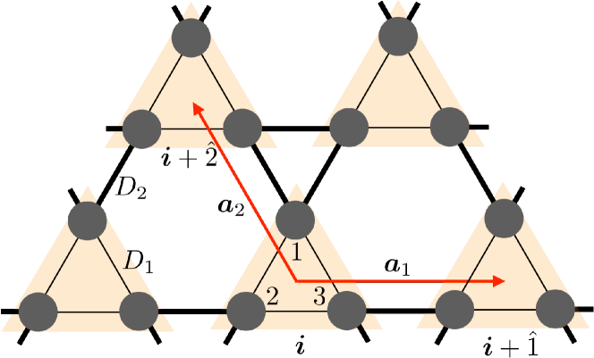
Figure 2: Nodes and bonds forming the kagome lattice. The orange triangle indicates the unit cell, and the red arrows are primitive translation vectors.

The breathing kagome lattice is one of the well-known examples of the HOTI Ezawa (2018) (See also Ref. Kheirkhah et al. (2022), which examined corner states of the kagome lattice in proximity to superconductors). Therefore, for the detection of the corner states, let us consider heat conduction on the breathing kagome lattice illustrated in Fig. 2, where we have defined the unit cell composed by three nodes specified by $a=1,2,3$. The primitive translation vectors are $\bm{a}_{1}$ and $\bm{a}_{2}$, and, in addition, $\bm{a}_{3}\equiv-(\bm{a}_{1}+\bm{a}_{2})$ is introduced, for convenience. These vectors have the same length $|\bm{a}_{j}|\equiv a$. We assume that all nodes are identical, whereas the bonds have two kinds of geometrical forms characterized by $A_{j}/L_{j}$ $(j=1,2)$, or two kinds of thermal conductivities, $k_{j}$ $(j=1,2)$, both of which yield two kinds of thermal diffusion constants $D_{j}$ ($j=1,2$). It follows from Eqs. (7) and (5) that the heat equation on the breathing kagome lattice is given by

$$\partial_{t}\phi_{a,\bm{i}}(t) =\sum_{b(\neq a)}\left[D_{1}(\phi_{b,\bm{i}}-\phi_{a,\bm{i}})-D_{2}(\phi_{a,\bm{i}}-\phi_{b,\bm{i}-\epsilon^{abc}\bm{a}_{c}})\right]$$

$$+\alpha(\phi_{0}^{4}-\phi_{a,\bm{i}}^{4}),$$ (11)

where

$$D_{j} \equiv\left\{\begin{array}[]{ll}\displaystyle\frac{k}{c\rho}\frac{A_{j}}{VL_{j}}\equiv\frac{d}{l_{j}^{2}}&\\ \mbox{or }&\quad(j=1,2),\\ \displaystyle\frac{k_{j}}{c\rho}\frac{A}{VL}\equiv\frac{d_{j}}{l^{2}}&\\ \end{array}\right.$$ (15)

$$\alpha =\frac{\varepsilon\sigma}{c\rho}\frac{S}{V}\delta T^{3}.$$ (16)

In this equation, we assume that $d$ or $d_{j}$ with some suitable renormalization denotes the conventional thermal diffusivity for the continuum system, and the parameter $l_{j}$ with the dimension of length characterizes the length scale of the present lattice system. Since we treat the nodes and bonds as simple points and lines, ignoring their geometric shapes, the model includes only the lattice constant $a$ which has the dimension of length. In what follows, we introduce the parametrization

$$D_{1}\equiv\frac{d_{1}}{a^{2}},\quad D_{2}\equiv\frac{d_{2}}{a^{2}},\quad(D_{1}=\delta D_{2})$$ (17)

using the lattice constant $a$ of the kagome lattice. Here, the parameter $\delta$ characterizes the topological phases of the breathing kagome lattice. Let us also define a typical time scale

$$\tau=\frac{1}{D}=\frac{a^{2}}{d},$$ (18)

where $D\equiv\min(D_{1},D_{2})$ and $d\equiv\min(d_{1},d_{2})$.

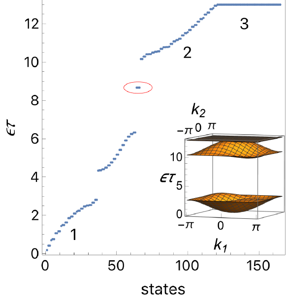
Figure 3: Spectrum of $\cal H$ in Eq. (9) for the breathing kagome lattice system (11) at $\delta=0.3$ of equilateral triangle with 10 unit cells per side. The threefold degenerate states encircled are corner states, other bands specified by numbers one, two, and three are the bulk bands, and the band with no number is due to the edge states. The inset shows the bulk spectrum.

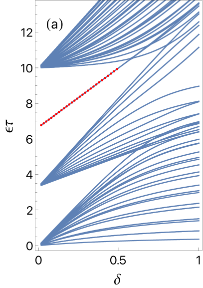
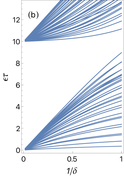
Figure 4: The spectrum of the same equilateral triangle system of Fig. 3 as a function of (a) $\delta$ and (b) $1/\delta$, where $\delta$ is defined in Eq. (17). The red dots indicate the corner states.

III.1 Spectrum of a finite system

This model show three bands, lowest and middle dispersive bands with a gap as well as a flat band at the top of the middle band (inset of Fig. 3). To investigate the corner states, let us consider the system of the triangle shape surrounded by heat bath, including $N$ nodes. For example, $N$ is given by $N=55\times 3=165$ for the triangle with ten unit cells per side. Figure 3 shows the spectrum for $\delta=0.3$ in the HOTI phase, where $\delta$ is defined in Eq. (17). We can see two dispersive bulk bands and a flat band, as well as threefold degenerate corner states and edge states in between the gap of dispersive bands one and two. We show in Fig. 4, the spectrum of $\cal H$ as a function of $\delta$. Since this model belongs to HOTI phase for $0<\delta<1/2$, it exhibits the corner states in this range Ezawa (2018). Even for $1/2<\delta<1$, there exist corner states, but embedded in the bulk upper band. For $1<\delta$, the model belongs to a trivial phase without corner states as shown in Fig. 4(b). Not only corner states but also edge states can be seen in Fig. 4(a), which are missing in the trivial regime in Fig. 4 (b).

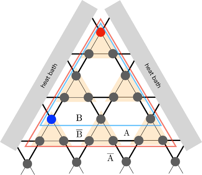
Figure 5: Top corner. The red and blue nodes are the nodes used for single-node measurement in Sec. III.2.1. The nodes surrounded by red (A) and blue (B) triangles are used for deriving effective Hamiltonians. Regions A and B include 18 and 12 nodes, respectively, in Sec. III.2.2.

III.2 Toward the detection of the corner states

Toward experimental detection of the corner states in the heat conduction system, we first consider the temperature measurement at one corner node Yoshida and Hatsugai (2021), which indeed reveals the existence of the corner states. Next, we discuss an improved way to determine the corner states by using data of temperature of several nodes around a corner which provides more accurate energy of the corner state. This may be called an effective Hamiltonian approach. For simplicity, we consider the case of $\alpha=0$.

III.2.1 Heat conduction at a corner

Assume that all the nodes are at the room temperature, $\phi_{\bm{i}}=0$. Let us give temperature $\phi_{\rm c}=1$ only at the corner node highlighted in red in Fig. 5 at time $t=0$, and measure how the given temperature decreases Yoshida and Hatsugai (2021). The result is shown in Fig. 6(a), in which one can see a clear distinction between the topological phase (solid curve) and trivial phase (dashed curve) in a short time regime. In particular, the heat conduction at the corner node is dominated in the topological phase by the corner state up to $t\sim\tau$. In passing, we point out that away from the corner but on the boundary highlighted by blue in Fig. 5, edge states can also be observed, as shown in Fig. 6(b). Indeed, the solid curve in the topological phase has clear difference from the dashed curve in the trivial phase. Its curvature also suggests the dispersive band for the edge states. For comparison, we show in Figs. 6(c) and 6(d) the temperature profiles on the lattice for the corner state and edge state, respectively.

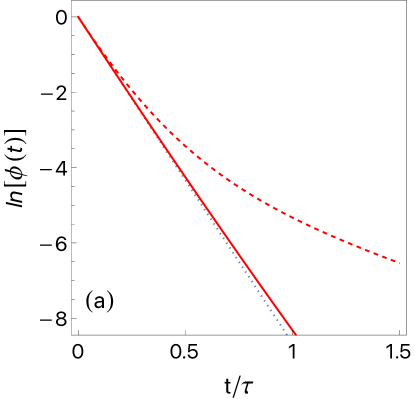
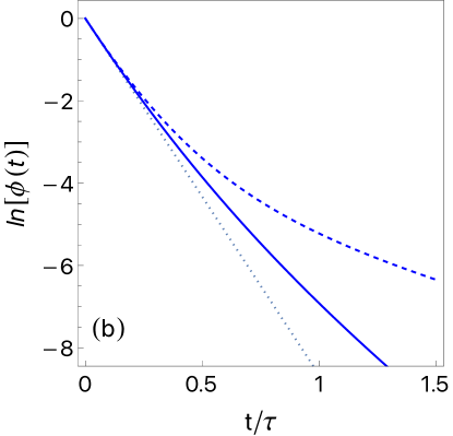
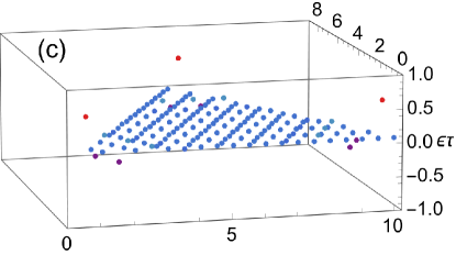
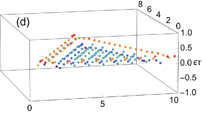
Figure 6: Single-node temperature as a function of $t/\tau$. (a) and (b) are the corner node and edge node highlighted in red and blue in Fig. 5, respectively. Full curves and dashed curves are the cases $\delta=0.3$ and $\delta=1/0.3$, respectively, which belong to the topological and trivial phases. Thin dotted lines are $-\varepsilon_{\rm c}t$, where $\varepsilon_{\rm c}$ is the energy of the corner states $\varepsilon_{\rm c}\tau=2(D_{1}+D_{2})/D$. (c) and (d) show the examples of the temperature profiles on the lattice for the corner states (No. 66) and edge states (No. 37, the lowest of the edge band), respectively, in the topological phase.

III.2.2 Effective Hamiltonian approach

So far we have shown that only one-node measurement of temperature is enough to detect the corner state in the heat conduction system. However, more precise determination of the energy of the corner state is achieved if one measures the temperature at more than one node Yoshida and Hatsugai (2021). To this end, let us prepare several initial distributions distinguished by index $p$. As in Eq. (9), we introduce the vector notation $\bm{\phi}_{p}$ whose components are $\phi_{\bm{i}p}(0)$. We assume that they are independent in the sense

$$\bm{\phi}_{p}^{T}\bm{\phi}_{q}=\delta_{pq}.$$ (19)

Since the local temperature $\phi_{\bm{i}}(t)$ depends on the initial distribution $\bm{\phi}_{p}$, let us denote $\phi_{\bm{i}p}(t)$, for which we also use the vector notation $\bm{\phi}_{p}(t)$. Then, the time evolution (10) is written as

$$\bm{\phi}_{p}(t)=\sum_{n}e^{-\varepsilon_{n}t}\bm{\phi}_{n}\bm{\phi}^{T}_{n}\bm{\phi}_{p}.$$ (20)

Taking the inner product with $\bm{\phi}_{q}$, we have Yoshida and Hatsugai (2021)

$${\cal T}_{pq}\equiv\bm{\phi}_{q}^{T}\bm{\phi}_{p}(t)=\bm{\phi}_{q}^{T}e^{-{\cal H}t}\bm{\phi}_{p}\equiv e^{-{\cal H}_{qp}t}.$$ (21)

The left hand side can be measured experimentally, whereas the right hand side tells how to compute the energy of the Hamiltonian $\cal H$. Namely, let $E_{n}$ be eigenvalues of the matrix $\cal T$. Then, the eigenvalues of $\cal H$ are given by $\varepsilon_{n}=-(\log E_{n})/t$. For a finite system with $N$ nodes, if we prepare $N$ independent initial temperature distributions and measure the temperature at all $N$ nodes, we can reproduce the exact energies shown in Fig. 3, as carried out in Yoshida and Hatsugai (2021).

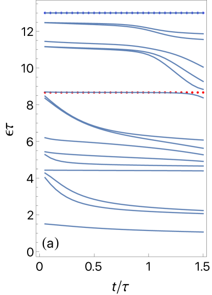
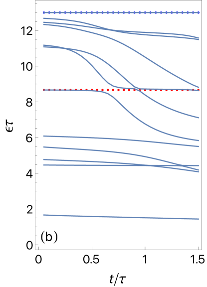
Figure 7: Spectra of effective Hamiltonian with restricted degrees of freedom as functions of time. (a) and (b) correspond to region A and B in Fig. 5. Red and blue dots denote the exact energy of the corner state and the flat band, respectively.

However, for the purpose of observing corner states and determining their energy, fewer initial conditions and fewer node temperature measurements are sufficient since each corner state is localized around each corner. Actually, in Sec. III.2.1, only one-node measurement at one corner with only one initial distribution enables to detect the existence of the corner mode. For such restricted measurements using reduced degrees of freedom, the energies, which should be constant along the time evolution, inevitably depend on time. Nevertheless, the energy of the corner states is almost constant. This is due to their localized nature. Thus, the time dependence of the energies could distinguish the energy of the corner state from those of other extended states.

For simplicity, we propose the following initial temperature distributions: We keep the temperature of all the nodes $\phi_{\bm{j}}=0$ except for that of node $\bm{i}$ which is set $\phi_{\bm{i}}=1$. The number of such initial distributions is of course $N$ and they satisfy Eq. (19). Here, we propose the restricted number of initial distributions to the nodes specified by triangles in Fig. 5. The whole system has 165 nodes, whereas the regions A and B include only 18 and 12 nodes, each of which is given the initial temperature $1$. Then, the measurements of the local temperature of each node in regions A and B at time $t$ allow us to calculate the energies of the reduced Hamiltonian. In Fig. 7, we show the energies of such a reduced Hamiltonian.

From the single-node measurement in Sec. III.2.1, we expect that the energies of the effective reduced Hamiltonian are decreasing as functions of time, since long-time behavior is controlled by low energy states, some of which are neglected in the reduced Hamiltonian. In Fig. 7, we plot the spectra of the reduce Hamiltonian for the restricted nodes in the A and B regions in Fig. 5. Indeed, Fig. 7 shows that all the energies are basically decreasing function. Among them, the energies which are nearly degenerate with the corner state at $t\sim 0$ are largely decreasing, as can be seen in Fig. 7(a). These are due to the states at the artificial boundary between A and $\overline{\mathrm{A}}$, which are connected by the large $D$ bonds. On the other hand, almost constant energies are due to the states which are not affected by the artificial boundary. The corner state may be the most typical state with such a property, because it has a localized temperature profile. Another typical state may be the flat band: Huge degeneracy enables to create a localized state by suitable linear combination of degenerate states, as indicated by blue dots in Fig. 7.

III.3 System with thermal radiation

Finally, we briefly discuss the effect of the thermal radiation. The Stefan-Boltzmann law gives rise to nonlinear effect term in Eq. (4). We solve such a nonlinear equation numerically, and apply the same procedure in Sec. III.2.2, which may serve as a mean field approximation. First of all, let us estimate the order of several parameters of the model.

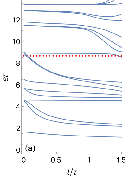
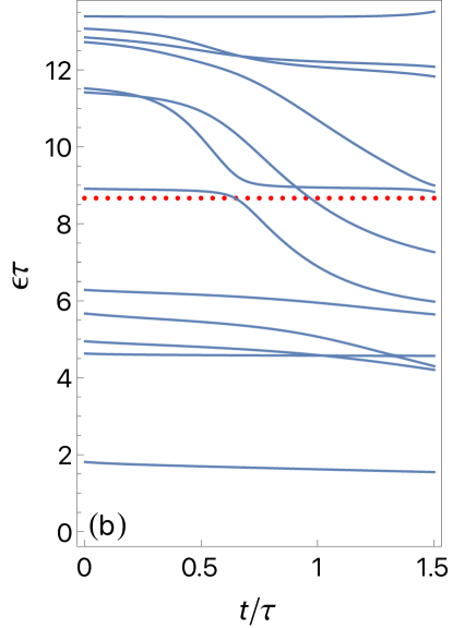
Figure 8: Same as Fig. 7 but with the Stefan-Boltzmann radiation with $\varepsilon=0.3$.

The implementation of the experiment in Ref. Hu et al. (2022) is such that the bonds have the area of the cross-section $A\sim 10^{-5}\,\hbox{m}^{2}$ and the length $L\sim 115\times 10^{-3}\,\hbox{m}$, and the nodes have the area of the surface $S\sim\pi R^{2}\sim 3\times 10^{-5}\,\hbox{m}^{2}$. The room temperature is $T_{0}=294\,\mbox{K}$ and $\delta T\sim 40\,\mbox{K}$, and hence, $\phi_{0}\sim 7.4$. From Eqs. (16) and (17), we have

$$\frac{\alpha}{D}=\frac{\varepsilon\sigma}{k}\frac{SL}{A}\delta T^{3}\sim 10^{-10}\varepsilon\delta T^{3}\sim 6.4\varepsilon\times 10^{-5},$$ (22)

where we have used $k=200\hbox{ W/m$\cdot$K}$ for aluminum, and the Stefan-Boltzmann constant $\sigma=5.7\times 10^{-8}\hbox{W/m${}^{2}$K${}^{4}$}$ with a relatively large emissivity $\varepsilon=0.3$. We calculate the energies as follows. Starting from the same initial condition used in Sec. III.2.2, solving the equations (11) numerically, and using data $\bm{\phi}_{p}(t)$, we compute the eigenvalues of $\cal T$ in Eq. (21), from which we deduce the energies in the same way in Sec. III.2.2. In Fig. 8, we show the energies thus computed in which small deviation can be seen, but basically, the effect of the thermal radiation is quite small even in a large emissivity. In the realistic case, at most $\varepsilon\sim 0.1$, and therefore, the thermal radiation may be negligible.

IV Summary

We proposed a higher-order topological heat conduction system toward the detection of the corner states. We first formulated generic heat conduction on a lattice composed of nodes and bonds, based on the Fourier law and energy conservation. Such a description indeed has an intimate relationship with the continuum heat conduction equation, as examined in the Appendix using a one-dimensional system with the SSH-like structure. We next applied to the breathing kagome lattice which is one of typical models showing HOTI phase. We showed that corner states can be observed by a simple measurement of the temperature only at one corner. We also proposed more precise measurement of the energy of the corner state using several nodes around a corner. Finally, the effect of the Stefan-Boltzmann thermal radiation was estimated, but this was found to be negligible.

In this paper, we showed that heat conduction on lattices is useful to detect topological properties for corresponding lattice systems. We also point out that heat transport from and to reservoirs can also be a useful probe for the same purposes Molignini et al. (2017). Thus, we expect that the heat conduction is much more useful than we expected to reveal directly or indirectly topological properties for various systems.

Appendix A Diffusion on a lattice as a discretization of the diffusion equation

We have introduced diffusion phenomena on a lattice composed of nodes and bonds. We show in this Appendix that such a description of diffusion phenomena can be regarded as a coarse discretization of the conventional diffusion equation if the diffusion constant of a lattice system is interpreted as an effective renormalized parameter. We show this fact using a simple 1D system with the SSH-like structure.

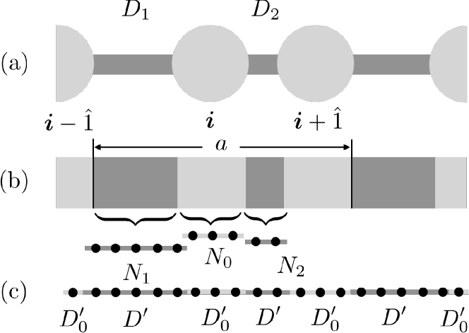
Figure 9: Schematic illustration of the 1D system. (a) Experimental implementation in Refs. Qi et al. (2022); Hu et al. (2022). (b) Corresponding continuum system obeying diffusion equation. (c) Discretized model of (b), which is numerically solved, instead of (b), in this Appendix.

The SSH-like structure for the heat conduction Yoshida and Hatsugai (2021) has been realized in experimental implementation (a) in Fig. 9 Qi et al. (2022); Hu et al. (2022), in which the nodes composed of cylindrical materials are connected by thin bonds whose large and small heat conductances are controlled by the length of the bonds. Apart from the geometric structure, the heat conduction on such a system may be basically described by the 1D diffusion equation for type (b) in Fig. 9, where the geometric structure of (a) is reflected by the assumption that the heat capacity of the nodes are very large in (a) and hence, the corresponding parts in (b) have very small heat conductivity. Instead of solving the continuum diffusion equation, we discretized (b) in fine meshes like (c) in Fig. 9. In this sense, the heat conduction on lattices in the text is the most coarse discretization of the diffusion equation.

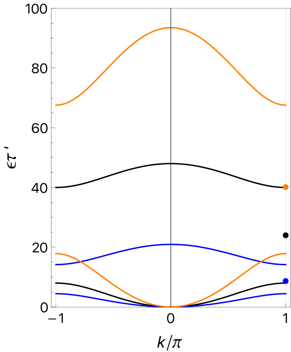
Figure 10: The bulk spectra (curves) and edge states (dots). Orange and blue are the cases of $(N_{1},N_{2},N_{0})=(50,10,5)$, $(20,4,4)$, whereas black is $(0,0,1)$, which is the simple SSH model in Fig. 9(a). The heat conductivities used are $(d,d_{0})=(1,10^{-2})$ for colored discretized models, whereas for the SSH model we have used $(D_{1},D_{2})=(0.2,1)$. As an effective energy we have used $1/\tau^{\prime}=d/(N_{1}a^{2})$ for the discretized models and $D_{1}/a^{2}$ for the SSH model, namely the smaller heat conductivity of the bonds.

The discretized Hamiltonian illustrated in Fig. 9(c) is given by

$$H\phi_{j} =-\partial^{*}D^{\prime}_{j}\partial\phi_{j}$$

$$=-[D^{\prime}_{j}\phi_{j+1}+D^{\prime}_{j-1}\phi_{j-1}-(D^{\prime}_{j}+D^{\prime}_{j-1})\phi_{j}],$$ (23)

where $\partial$ and $\partial^{*}$ stand for the forward and backward difference operators, $\partial f_{j}=f_{j+1}-f_{j}$ and $\partial^{*}f_{j}=f_{j}-f_{j-1}$, respectively, and

$$D^{\prime}_{j}=\left\{\begin{array}[]{ll}\displaystyle D^{\prime}\equiv d/a_{0}^{2}&(j\in\mbox{ bonds})\\ \displaystyle D^{\prime}_{0}\equiv d_{0}/a_{0}^{2}&(j\in\mbox{ nodes})\end{array}\right..$$ (26)

In the above, $a_{0}=a/(N_{1}+N_{2}+2N_{0})$ is the artificial lattice constant of the mesh in (c), where $a$ is the length of the unit cell. Here we assume that $d_{0}\ll d$, since the heat capacity of the nodes are very large, as mentioned above. Note here that the bonds have the same heat conductivity $D^{\prime}$, and the difference of $D_{1}$ and $D_{2}$ for the SSH heat conduction model is due to the difference of the lengths of the bonds, $N_{1}$ and $N_{2}$.

In Fig. 10, we show some examples of the bulk spectra as well as the edge states restricted to the two lowest energy bands. Here, the edge states are computed by the method proposed in Ref. Fukui (2020). The numbers of meshes in a unit cell are $70$ (orange), $34$ (blue), and $2$ (black). The last one corresponds to the SSH heat conduction model Yoshida and Hatsugai (2021); Hu et al. (2022). One can indeed see that the most coarse lattice model can describe very well the fine-mesh model close to the continuum heat conduction equation, including the edge states. Of course, if one wants to finetune the energies, one should regard $\tau^{\prime}$ as a parameter, or use renormalized diffusion conductivities.

References

- Hatsugai (1993a) Y. Hatsugai, Physical Review Letters 71, 3697 (1993a), URL http://link.aps.org/doi/10.1103/PhysRevLett.71.3697.
- Hatsugai (1993b) Y. Hatsugai, Physical Review B 48, 11851 (1993b), URL https://link.aps.org/doi/10.1103/PhysRevB.48.11851.
- Kane and Mele (2005a) C. L. Kane and E. J. Mele, Physical Review Letters 95, 146802 (2005a), URL http://link.aps.org/doi/10.1103/PhysRevLett.95.146802.
- Kane and Mele (2005b) C. L. Kane and E. J. Mele, Physical Review Letters 95, 226801 (2005b), URL http://link.aps.org/doi/10.1103/PhysRevLett.95.226801.
- Qi et al. (2008) X.-L. Qi, T. L. Hughes, and S.-C. Zhang, Physical Review B 78, 195424 (2008), URL http://link.aps.org/doi/10.1103/PhysRevB.78.195424.
- Hasan and Kane (2010) M. Z. Hasan and C. L. Kane, Reviews of Modern Physics 82, 3045 (2010), URL http://link.aps.org/doi/10.1103/RevModPhys.82.3045.
- Qi and Zhang (2011) X.-L. Qi and S.-C. Zhang, Reviews of Modern Physics 83, 1057 (2011), URL http://link.aps.org/doi/10.1103/RevModPhys.83.1057.
- Raghu and Haldane (2008) S. Raghu and F. D. M. Haldane, Physical Review A 78, 033834 (2008), URL https://link.aps.org/doi/10.1103/PhysRevA.78.033834.
- Haldane and Raghu (2008) F. D. M. Haldane and S. Raghu, Physical Review Letters 100, 013904 (2008), URL https://link.aps.org/doi/10.1103/PhysRevLett.100.013904.
- Wang et al. (2009) Z. Wang, Y. Chong, J. D. Joannopoulos, and M. Soljačić, Nature 461, 772 EP (2009), URL https://doi.org/10.1038/nature08293.
- Ozawa et al. (2019) T. Ozawa, H. M. Price, A. Amo, N. Goldman, M. Hafezi, L. Lu, M. C. Rechtsman, D. Schuster, J. Simon, O. Zilberberg, et al., Reviews of Modern Physics 91, 015006 (2019), URL https://link.aps.org/doi/10.1103/RevModPhys.91.015006.
- Kivshar (2019) Y. Kivshar, Low Temperature Physics 45, 1026 (2019), URL https://doi.org/10.1063/1.5121273.
- Prodan and Prodan (2009) E. Prodan and C. Prodan, Physical Review Letters 103, 248101 (2009), URL https://link.aps.org/doi/10.1103/PhysRevLett.103.248101.
- Savin et al. (2010) A. V. Savin, Y. S. Kivshar, and B. Hu, Physical Review B 82, 195422 (2010), URL https://link.aps.org/doi/10.1103/PhysRevB.82.195422.
- Kane and Lubensky (2013) C. L. Kane and T. C. Lubensky, Nature Physics 10, 39 EP (2013), URL https://doi.org/10.1038/nphys2835.
- Kariyado and Hatsugai (2015) T. Kariyado and Y. Hatsugai, Scientific Reports 5, 18107 EP (2015), URL https://doi.org/10.1038/srep18107.
- Süsstrunk and Huber (2015) R. Süsstrunk and S. D. Huber, Science 349, 47 (2015), URL https://science.sciencemag.org/content/sci/349/6243/47.full.pdf.
- Chien et al. (2018) C.-C. Chien, K. A. Velizhanin, Y. Dubi, B. R. Ilic, and M. Zwolak, Physical Review B 97, 125425 (2018), URL https://link.aps.org/doi/10.1103/PhysRevB.97.125425.
- Yoshida and Hatsugai (2019) T. Yoshida and Y. Hatsugai, Physical Review B 100, 054109 (2019), URL https://link.aps.org/doi/10.1103/PhysRevB.100.054109.
- Albert et al. (2015) V. V. Albert, L. I. Glazman, and L. Jiang, Physical Review Letters 114, 173902 (2015), URL https://link.aps.org/doi/10.1103/PhysRevLett.114.173902.
- Lee et al. (2018) C. H. Lee, S. Imhof, C. Berger, F. Bayer, J. Brehm, L. W. Molenkamp, T. Kiessling, and R. Thomale, Communications Physics 1, 39 (2018), URL https://doi.org/10.1038/s42005-018-0035-2.
- Helbig et al. (2020) T. Helbig, T. Hofmann, S. Imhof, M. Abdelghany, T. Kiessling, L. W. Molenkamp, C. H. Lee, A. Szameit, M. Greiter, and R. Thomale, Nature Physics 16, 747 (2020), URL https://doi.org/10.1038/s41567-020-0922-9.
- Yoshida et al. (2020) T. Yoshida, T. Mizoguchi, and Y. Hatsugai, Physical Review Research 2, 022062 (2020), URL https://link.aps.org/doi/10.1103/PhysRevResearch.2.022062.
- Delplace et al. (2017) P. Delplace, J. B. Marston, and A. Venaille, Science 358, 1075 (2017), URL https://science.sciencemag.org/content/sci/358/6366/1075.full.pdf.
- Sone and Ashida (2019) K. Sone and Y. Ashida, Physical Review Letters 123, 205502 (2019), URL https://link.aps.org/doi/10.1103/PhysRevLett.123.205502.
- Li et al. (2019) Y. Li, Y.-G. Peng, L. Han, M.-A. Miri, W. Li, M. Xiao, X.-F. Zhu, J. Zhao, A. Alù, S. Fan, et al., Science 364, 170 (2019), eprint https://www.science.org/doi/pdf/10.1126/science.aaw6259, URL https://www.science.org/doi/abs/10.1126/science.aaw6259.
- Yoshida and Hatsugai (2021) T. Yoshida and Y. Hatsugai, Scientific Reports 11, 888 (2021), URL https://doi.org/10.1038/s41598-020-80180-w.
- Su et al. (1979) W. P. Su, J. R. Schrieffer, and A. J. Heeger, Physical Review Letters 42, 1698 (1979), URL https://link.aps.org/doi/10.1103/PhysRevLett.42.1698.
- Qi et al. (2022) M. Qi, D. Wang, P.-C. Cao, X.-F. Zhu, C.-W. Qiu, H. Chen, and Y. Li, Advanced Materials 34, 2202241 (2022), eprint https://onlinelibrary.wiley.com/doi/pdf/10.1002/adma.202202241, URL https://onlinelibrary.wiley.com/doi/abs/10.1002/adma.202202241.
- Hu et al. (2022) H. Hu, S. Han, Y. Yang, D. Liu, H. Xue, G.-G. Liu, Z. Cheng, Q. J. Wang, S. Zhang, B. Zhang, et al., Advanced Materials 34, 2202257 (2022), URL https://doi.org/10.1002/adma.202202257.
- Makino et al. (2022) S. Makino, T. Fukui, T. Yoshida, and Y. Hatsugai, Physical Review E 105, 024137 (2022), URL https://link.aps.org/doi/10.1103/PhysRevE.105.024137.
- Slager et al. (2015) R.-J. Slager, L. Rademaker, J. Zaanen, and L. Balents, Physical Review B 92, 085126 (2015), URL https://link.aps.org/doi/10.1103/PhysRevB.92.085126.
- Hashimoto and Kimura (2016) K. Hashimoto and T. Kimura, Physical Review B 93, 195166 (2016), URL https://link.aps.org/doi/10.1103/PhysRevB.93.195166.
- Kunst et al. (2017) F. K. Kunst, M. Trescher, and E. J. Bergholtz, Physical Review B 96, 085443 (2017), URL https://link.aps.org/doi/10.1103/PhysRevB.96.085443.
- Benalcazar et al. (2017a) W. A. Benalcazar, B. A. Bernevig, and T. L. Hughes, Science 357, 61 (2017a), URL http://science.sciencemag.org/content/sci/357/6346/61.full.pdf.
- Benalcazar et al. (2017b) W. A. Benalcazar, B. A. Bernevig, and T. L. Hughes, Physical Review B 96, 245115 (2017b), URL https://link.aps.org/doi/10.1103/PhysRevB.96.245115.
- Hashimoto et al. (2017) K. Hashimoto, X. Wu, and T. Kimura, Physical Review B 95, 165443 (2017), URL https://link.aps.org/doi/10.1103/PhysRevB.95.165443.
- Kunst et al. (2018) F. K. Kunst, G. van Miert, and E. J. Bergholtz, Physical Review B 97, 241405 (2018), URL https://link.aps.org/doi/10.1103/PhysRevB.97.241405.
- Schindler et al. (2018) F. Schindler, A. M. Cook, M. G. Vergniory, Z. Wang, S. S. P. Parkin, B. A. Bernevig, and T. Neupert, Science Advances 4, eaat0346 (2018), URL https://advances.sciencemag.org/content/advances/4/6/eaat0346.full.pdf.
- Ezawa (2018) M. Ezawa, Physical Review Letters 120, 026801 (2018), URL https://link.aps.org/doi/10.1103/PhysRevLett.120.026801.
- Imhof et al. (2018) S. Imhof, C. Berger, F. Bayer, J. Brehm, L. W. Molenkamp, T. Kiessling, F. Schindler, C. H. Lee, M. Greiter, T. Neupert, et al., Nature Physics 14, 925 (2018), URL https://doi.org/10.1038/s41567-018-0246-1.
- Zhang et al. (2019) X. Zhang, H.-X. Wang, Z.-K. Lin, Y. Tian, B. Xie, M.-H. Lu, Y.-F. Chen, and J.-H. Jiang, Nature Physics 15, 582 (2019), URL https://doi.org/10.1038/s41567-019-0472-1.
- Ota et al. (2019) Y. Ota, F. Liu, R. Katsumi, K. Watanabe, K. Wakabayashi, Y. Arakawa, and S. Iwamoto, Optica 6, 786 (2019), URL http://www.osapublishing.org/optica/abstract.cfm?URI=optica-6-6-786.
- Kheirkhah et al. (2022) M. Kheirkhah, D. Zhu, J. Maciejko, and Z. Yan, Phys. Rev. B 106, 085420 (2022), URL https://link.aps.org/doi/10.1103/PhysRevB.106.085420.
- Molignini et al. (2017) P. Molignini, E. van Nieuwenburg, and R. Chitra, Phys. Rev. B 96, 125144 (2017), URL https://link.aps.org/doi/10.1103/PhysRevB.96.125144.
- Fukui (2020) T. Fukui, Physical Review Research 2, 043136 (2020), URL https://link.aps.org/doi/10.1103/PhysRevResearch.2.043136.