Odd-parity perturbations of the wormhole-like geometries and quasi-normal modes in Einstein-Æther theory
Abstract
The Einstein-ther theory has drawn a lot of attentions in recent years. As a representative case of gravitational theories that break the Lorentz symmetry, it plays an important role in testing the Lorentz-violating effects and shedding light on the attempts to construct quantum gravity. Since the first detection to the gravitational wave, the event GW150914, a brand new window has been opened to testing the theory of gravity with gravitational wave observations. At the same time, the study of gravitational waves itself also provides us a serendipity of accessing the nature of a theory. In this paper, we focus on the odd-parity gravitational perturbations to a background that describes a wormhole-like geometry under the Einstein-ther theory. Taking advantage of this set of analytic background solutions, we are able to simplify the Lagrangian and construct a set of coupled single-parameter dependent master equations, from which we solve for the quasi-normal modes that carry the physical information of the emitted gravitational waves. Basically, the results reflect a consistency between Einstein-ther theory and general relativity. More importantly, as long as the no-ghost condition and the latest observational constraints are concerned, we notice that the resultant quasi-normal mode solutions intimate a kind of dynamical instability. Thus, the solutions are ruled out based on their stability against small linear perturbations.
I Introduction
The detection of the first gravitational wave (GW) from the coalescence of two massive black holes (BHs) by advanced LIGO/Virgo marked the beginning of a new era — the GW astronomy Ref1 . Following this observation, about 90 GW events have been identified by the LIGO/Virgo/KAGRA (LVK) scientific collaborations (see, e.g., GWs ; GWs19a ; GWs19b ; GWsO3b ). In the future, more ground- and space-based GW detectors will be constructed Moore2015 ; Gong:2021gvw , which will enable us to probe signals with a much wider frequency band and larger distances. This triggered the interest in the quasi-normal mode (QNM) of black holes, as GWs emitted in the ringdown phase can be considered as the linear combination of these individual modes Berti2009 ; Berti18 . Similarly, attention has been paid in recent years to QNM originating from wormholes Kono2018 ; Volkel2018 ; Kim2018 ; Franzin2022 .
From the classical point of view, QNMs are eigenmodes of dissipative systems. The information contained in QNMs provides the keys to revealing whether BHs are ubiquitous in our universe, and more important whether general relativity (GR) is the correct theory to describe gravity even in the strong field regime Berti18b . Basically, a QNM frequency contains two parts, the real and imaginary parts. Its real part gives the vibration frequency while its imaginary part provides the damping time.
In GR, according to the no-hair theorem, an isolated and stationary BH is completely characterized by only three quantities, mass, angular momentum, and electric charge. Astrophysically, we expect BHs to be neutral, so they are uniquely described by the Kerr solution. Then, the QNM frequencies and damping times will depend only on the mass and angular momentum of the finally formed BH. Clearly, to extract physics from the ringdown phase, at least two QNMs are needed. This will require the signal-to-noise ratio (SNR) to be of the order 100 Berti18 . Although such high SNRs are not achievable right now, it has been shown that they may be achievable once the advanced LIGO, Virgo, and KAGRA reach their fully designed sensitivities. In any case, it is certain that they will be detected by the ground-based third-generation detectors, such as Cosmic Explorer CE and the Einstein Telescope ET , as well as the space-based detectors, including LISA LISA , TianQin Liu2020 ; Shi2019 , Taiji Taiji2 , and DECIGO DECIGO .
QNMs in GR have been studied extensively Chandra92 , including scalar, vector, and tensor perturbations Iyer1987 . Such calculations have been extended from the Schwarzschild BH to other more general cases, e.g., the Kerr BH Det1980 ; Seidel1990 . In this procedure, several different techniques of computations of QNMs were developed. For instance, the Wentzel-Kramers-Brillouin (WKB) approach Will1985 ; Will1987 ; Konoplya2003 ; Jerzy2017 , the finite difference method (FDM) XinLi2020 , the continued fraction method Leaver1985 , the shooting method Chandra1975 ; Doneva2010 , the matrix method Kai2017 , and so on Kono2011 ; Gund1994 ; Bin2004 . Some of these methods have also been applied to modified theories of gravity XinLi2020 ; Oliver2019 ; KZ07b . In addition, some special approximations, e.g., the eikonal limit, have also been extensively explored, see, for example, Ref. Huan2012 and references therein.
This paper focuses on the QNM problem in Einstein-Æther theory. A set of analytic background solutions describing a throat geometry in the Einstein-Æther theory will be considered, and the odd-parity perturbations will be investigated. Such studies are well-motivated. In particular, the Einstein-Æther theory is self-consistent, such as free of ghosts and instability Jacobson , and satisfies all the experimental tests carried out so far OMW18 ; Tsujikawa21 . Its Cauchy problem is also well-posed SBP19 , and energy is always positive (as far as the hypersurface-orthogonal æther field is concerned) GJ11 .
In comparison with other modified theories of gravity CFPS12 , including scalar-tensor theories and their high-order corrections DL19 , Einstein-Æther theory has the following distinguishable features: It is a particular vector-tensor theory in which the vector field is always timelike. As a result, it always defines a preferred frame and whereby violates locally the Lorentz invariance (LI). Despite the facts that LI is the cornerstone of modern physics, and all the experiments carried out so far are consistent with it Bourgoin21 ; Bars19 ; Shao19 ; Bourgoin17 ; Flowers17 ; KR11 , violations of LI have been well motivated and extensively studied in the past several decades, especially from the point of view of quantum gravity Collin04 ; Mattingly05 ; Liberati13 ; PT14 ; Wang17 . In Einstein-Æther theory there exist three different species of gravitons, spin-0, spin-1, and spin-2, and each of them propagates at different speeds JM04 . To avoid the vacuum gravi-Čerenkov radiation, such as cosmic rays, each of these three species must move with a speed that is at least no less than the speed of light EMS05 . As a matter of fact, depending on the choice of the free coupling constants of the theory, they can be arbitrarily large, and so far no upper limit of these speeds are known KR11 .
With the above remarkable features of the Einstein-Æther theory, it is interesting and important to find new predictions of the theory for the QNMs mentioned above. The BH spectroscopy Berti18 has been extensively studied in the last couple of years in terms of GWs emitted in the ringdown phase of binary BHs (BBHs) (for example, see BLT21 ; LCV20 ; FBPF20 ; BFPF20 ; GST19 ; IGFST19 ; CDV19 ; CN20 ; OC20 ; Shaik20 ; Uchi20 ; BCCK20 ; Cabero20 ; Maselli20 ; Islam20 and references therein), and found that they are all consistent with GR within the error bars allowed by the observations of the 90 GW events LVK2022 . And here, as mentioned earlier, we shift our insights to the study of wormholes and throat geometries in the Einstein-Æther theory.
The rest of the paper is organized as follows. In Sec. II we provide a brief introduction to the Einstein-Æther theory. Fundamental definitions will be given and the background solutions of throat geometries will be discussed. After that, a demonstration of simplifying the odd-parity perturbed Lagrangian under the so-called isotropic coordinate is given in Sec. III. On top of that, we are ready to process the derivations of QNM in Sec. IV. The basic steps of calculations and main results are shown in there. With the results, some concluding remarks are addressed in Sec. V.
We shall adopt the unit system so that , where is the speed of light and is the Newtonian gravitational constant [It’s worth mentioning here that, after this, we still have one degree of freedom (d.o.f) in choosing the unit system for ]. We will also work with the signature . All the Greek letters run from 0 to 3.
II Einstein-Æther theory
In Einstein-Æther theory (-theory), the fundamental variables of the gravitational sector are Jacobson ,
| (2.1) |
where is the four-dimension metric of the spacetime, is the æther field, and is a Lagrangian multiplier, which guarantees that the æther field is always timelike and unity. Then, the general action of the theory is given by,
| (2.2) |
where denotes the action of matter, and the gravitational action of the -theory, given, respectively, by
| (2.3) |
Here collectively denotes the matter fields, and is the determinant of , and
| (2.4) |
where denotes the covariant derivative with respect to , is the Ricci scalar, and is defined as
with representing the Kronecker delta. Note that here we assume that matter fields couple not only to but also to the æther field . However, in order to satisfy the severe observational constraints, such a coupling, in general, is assumed to be absent Jacobson .
The four coupling constants ’s are all dimensionless, and is related to the Newtonian gravitational constant via the relation CL04 ,
| (2.6) |
where .
II.1 Field Equations
The variations of the total action, respectively, with respect to , and yield respectively the field equations Chao2020b ,
| (2.7) | |||||
| (2.8) | |||||
| (2.9) |
where denotes the Ricci tensor, and
| (2.10) |
with
| (2.11) |
From Eq.(2.8), we find that
| (2.12) |
where . Notice that, by considering only the vacuum solutions (as what we will do later), the matter fields disappear, leading to the absence of as well as in Eqs. (2.7) and (2.8).
It is easy to show that the Minkowski spacetime is a solution of -theory, in which the æther is aligned along the time direction, . Then, the linear perturbations around the Minkowski background show that the theory in general possesses three types of excitations, scalar (spin-0), vector (spin-1), and tensor (spin-2) modes, with their squared speeds given by JM04
| (2.13) |
respectively. Here .
Requiring that the theory: 1) be self-consistent, such as free of ghosts; and 2) satisfies all the observational constraints obtained so far, it was found that the parameter space of the theory is considerably restricted. In particular, , and are restricted to OMW18 222The recent studies of the neutron binary systems showed that the PPN parameter is further restricted to GHBBCYY , which is an order of magnitude stronger than the bounds from lunar laser ranging experiments MWT08 . This will translate the constraint on given by Eq.(2.14) to , as one can see clearly from Eq.(3.12) given in OMW18 .,
| (2.14) | |||
| (2.15) | |||
| (2.16) |
Taking , the stability of the odd-parity perturbations of BHs further requires Tsujikawa21 .
II.2 Background Geometry
From now on, we shall consider solely the vacuum solutions to the field equations [cf., Eqs.(2.7)-(2.9)]. For later convenience, in this subsection, we shall first adopt the isotropic coordinate, represented by (see, e.g., §8.2 of Weinberg1972 ). Thus, for the spherically symmetric time-independent case, the background line element and the æther field are given by Jacob2021
| (2.17) |
where .
As pointed in Jacob2021 , substituting (II.2) into Eq.(2.7), and picking up the - 333Notice that, in Jacob2021 the coordinate “” was written as “”. and -components, we obtain
| (2.18) |
where a prime in the superscript expediently stands for the derivative respective to .
Clearly, a master equation could be easily constructed from Eq.(II.2). As shown in Jacob2021 , that leads to the solutions
| (2.19) |
where [cf., Eq.(2.14) and footnote #1] and Weinberg1972 ; Jacob2021 . Note that, the solutions in (II.2) are characterized by a single parameter . In addition, they describe a throat geometry. As long as , a marginally trapped throat with a finite non-zero radius always exists, and on one side of it the spacetime is asymptotically flat, while on the other side, the spacetime becomes singular within a finite proper distance from the throat Jacob2021 .
When moving to the Schwarzschild coordinate, represented by , the line element could be written as
| (2.20) | |||||
which will immediately go back to that of GR at the limit Jacob2021 .
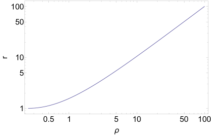
Notice that, a simple relation between and is given by Weinberg1972
| (2.21) |
To make it more clear, we show the relation between and in Fig. 1, in which we set .
III The odd-parity perturbations
In this section, we move to the odd-parity perturbations to the background described by Eq.(II.2). The full metric and æther field are given like
| (3.1) |
Here, the and denote the background fields, described by Eq.(II.2), while stands for an infinitesimal constant.
Firstly, we shall keep working in the isotropic coordinate. By mimicking Thomp2017 , the perturbation terms could be written as
| (3.2) |
and
| (3.3) |
where , , and are functions of and 444 It must not be confused with the function introduced here and the tensor appearing in Eq.(II.1)., while denotes the spherical harmonics. Starting from now on, we shall set in the above expressions so that , as now the background has the spherical symmetry, and the corresponding linear perturbations do not depend on Regge57 ; Thomp2017 555Notice that, since we are using the isotropic coordinate and following some different conventions, the terms in (3.2) are not necessarily equal to their counterparts given in Thomp2017 ..
III.1 Gauge Transformations and Gauge Fixing
For later convenience, we here investigate the infinitesimal gauge transformations (Recall that we only consider the odd-parity perturbations and )
| (3.4) |
where
| (3.5) |
with being a function of and . Under the transformation of Eq.(3.4), we have
| (3.6) |
where stands for the Lie derivative Invb . From Eq.(III.1) we find
| (3.7) | |||||
where a prime and a dot stand for the derivatives with respect to and , respectively. With the above gauge transformations, we can construct the gauge-invariant (GI) quantities, and due to the presence of the æther field, three such independent quantities can be constructed, in contrast to the relativistic case, in which only two such quantities can be constructed. These three gauge invariants can be defined as
| (3.8) |
Of course, any combination of these quantities is also GI. According to Eq.(III.1), by simply choosing the gauge condition (This could be referred as the RW gauge Thomp2017 ), and will reduce to and , respectively. This will be the gauge condition that we shall adopt in the following of this paper.
III.2 Simplified Lagrangian
To derive the partial differential equations (PDEs) for the perturbations, we need to first simplify the original Lagrangian, adopted in (2.2). Up to the 2nd order of , the total action can be cast in the form
| (3.9) |
Following Tsujikawa21 , we substitute (III) [together with Eqs.(II.2), (3.2) and (3.3)] into (2.2), and then pick up the terms. In addition, from now on, we shall set
| (3.10) |
since it has been confined to an extremely narrow region [cf., (2.16)]. The resultant 2nd-order action is given by
| (3.11) | |||
| (3.12) |
Notice that, the Lagrangian is only a function of and , as and have been integrated out, during which procedure, the features of spherical harmonics have been used intensively (see Appendix A).
With the help of integration by parts Arfken , plus the background field equations [cf., (2.7)-(2.9)], the quantity is simplified to
| (3.13) | |||||
where
which could be matched to its counterpart in Tsujikawa21 . Recall that , and (as well as their combination ) are GI under the chosen gauge condition, viz., [cf., Eq.(III.1)]. Note that, before stimulating any confusion, we shall omit the subscript for . The coefficients ’s are functions of , , , , etc. We abbreviate their full expressions since they are only for the narration of intermediate steps.
In (3.13), the apparent d.o.f for the odd-parity perturbations is 3, spanned by . However, the true d.o.f is 2 Tsujikawa21 . To get rid of that redundant d.o.f, we apply the Euler-Lagrange (E-L) equation Taylor05 to with respect to and , and obtain
| (3.15) |
where we have defined . Substitute (III.2) into the second line of (3.13), together with some rearrangements, becomes
| (3.16) | |||||
The coefficients ’s could be found in Appendix B. Clearly, as promised earlier, the current apparent d.o.f for the 2nd-order Lagrangian is 2, spanned by .
IV Quasi-normal modes of the odd-parity perturbations
IV.1 Master Equations
Combining (3.12) and (3.16), we obtain the simplified 2nd-order Lagrangian for the case. Now we are ready to derive the master equation for calculating the QNMs. With this Lagrangian, we apply the E-L equation to it with respect to and . That leads to a set of coupled PDEs
| (4.1) |
where a prime in the superscript expediently denotes the derivative with respect to . The expressions of ’s could be found in Appendix C.
In the next step, we shall apply the analytic solutions (II.2), and transfer our PDEs from the isotropic coordinate to the Schwarzschild coordinate . In addition, taking advantage of the residual d.o.f for choosing the unit system, we further set (so that the unit system of is totally fixed). By doing so, the PDEs are translated to
| (4.2) | |||||
where a prime in the superscript now stands for the derivative with respect to . A dot, as usual, stands for the derivative with respect to .
In writing down Eq.(IV.1), the stability condition of BHs that found in Tsujikawa21 , viz., , needs to be considered [so that the only theory-dependent coupling constant of Eq.(IV.1) is (or equivalently, ), since now we have ]. By performing suitable coordinate transformations, the PDEs in (IV.1) could be further translated to [the formulas in Appendix D were used in deriving Eqs.(4.3) and (4.4)]
| (4.3) | |||||
| (4.4) |
where
| (4.5) |
and
| (4.6) |
It’s worth mentioning here that, at the limit, Eq.(4.3) will reduce precisely to that of GR (see, e.g., the Eq.(2.13) of Kono2011 ).
IV.2 Calculate for the QNMs
As has been shown, taking brings us the coupled PDEs, Eqs.(4.3) and (4.4). With the above master equations, we are now at the stage of solving them for QNMs. To deal with this set of coupled PDEs, we shall apply the finite difference method (FDM) XinLi2020 ; Habermanb . By working with the FDM, we are expecting to solve (4.3) and (4.4) for . The solved will carry the information of QNM frequency (see, e.g., Berti2009 for a review). Notice that, can only reflect the comprehensive effects of all the existing ’s and it’s not trivial to extract individual ’s from .
To perform FDM, we shall basically follow Habermanb ; Kai2016 , and obtain the recursion formula
| (4.7) | |||||
where and are the step sizes for the and directions, respectively. They will be assigned suitable values in practice according to our usage. Here, denote the speed factor in front of the terms. Of course, for PDEs like Eqs.(4.3) and (4.4) we have .
The calculations of will be performed on a isosceles triangular lattice in the Cartesian coordinate system. The bottom side of the triangle contains points so that , where is a positive integer that will be chosen properly according to our usage. The height of the triangle contains points so that . After iterations, and with apt initial conditions, the functions could be obtained numerically. In practice, the initial conditions are chosen to be XinLi2020 ; Kai2016
| (4.8) |
 |
 |
 |
| (a) | (b) | (c) |
 |
 |
 |
| (d) | (e) | (f) |
 |
 |
 |
| (g) | (h) | (i) |
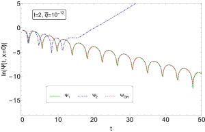
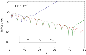
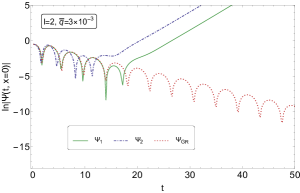
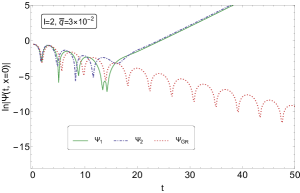
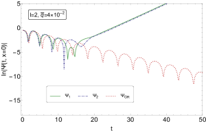
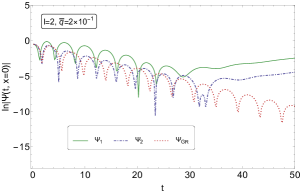
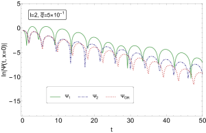
Due to the observational significance of the mode Mag18 ; Shi2019 ; Ghosh2021 ; LVK2022 , we shall mainly focus on this case (Of course, the computations and analysis here could be easily extended to higher ’s). The main results of the corresponding solutions are exhibited in Fig. 2. In there we plot out the temporal evolution of , together with the GR case as a comparison. Recall that we are adopting the unit system so that . To show it more explicit how the magnitude of influences the behaviors of , we considered both physically allowed and forbidden ’s. Based on Fig. 2, we have the following comments:
-
•
From panel (a) to panel (i), the value of is increasing. We observed that, in general, the behavior of is quite different from that of , which makes sense since the former is mainly from the gravitational perturbations [the contributions from the æther field to is suppressed by the small factor , as seen from the definition (III.2)] while the latter represents the contributions of the æther field.
-
•
When is small enough [e.g., panel (a)], the curve of is almost overlapped with that of GR. In contrast, when is large [e.g., panel (i)], the curve of will deviate a lot from that of GR. Of course, these are what we expected.
-
•
As approaching [cf., panels (a)-(d)], the deformation on the curve of tends to disappear. This makes sense since and are of the form for a tiny [cf., (IV.1)].
-
•
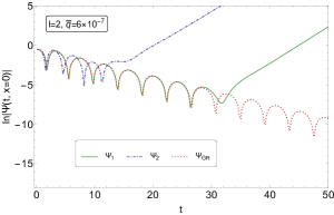
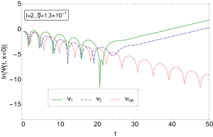
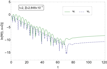
In panels (d)-(i), physically forbidden ’s were used [cf., Eq.(2.14)]. Even though, from there we see clearly how the dynamical instability arises. When is large enough, behaves in a healthy way [e.g., panel (i)]. However, for small enough ’s, will finally blow up, which reflects the existence of a dynamical instability Konoplya2018 [e.g., panel (g)]. As could be estimated, the critical point should occur at [cf., panels (h) and (i)].
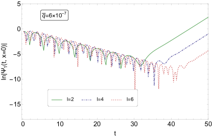
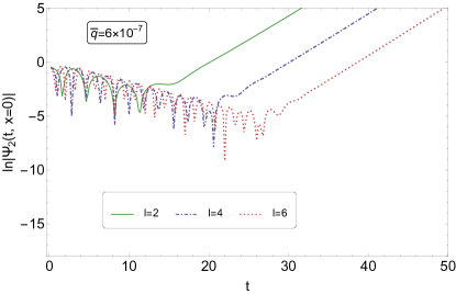
Since the position of the critical point has special significance, we carry out a more careful investigation of that. By selecting a near the critical point, the curves of are shown in Fig. 3 with a larger scope of . In there we observe the plateaux appearing on the curves of , which, from the phenomenological point of view, indicates that the current is around the critical point Kai2016 .
-
•
In contrast, physically allowed ’s [cf., Eq.(2.14)] were selected for panels (a)-(c). Although will blow up soon or later, we observe that the curves of ’s are almost overlapped with that of GR, before blowing up. That makes sense since those physically allowed ’s are extremely small, and means the GR limit.
-
•
From panels (a)-(h), we noticed that the times of blowing up for are getting earlier and earlier simultaneously as getting smaller from a big enough value [cf., panel (h)]. This tendency vaporizes at , where and exchange their chronological order of blowing up [cf., panels (e) and (f)]. Starting from this point, the curve of is getting frozen step by step [cf., panels (d) and (e)], and tends to lose its sensitivity on the magnitude of [cf., panels (a)-(d), as mentioned earlier]. While for the curve of , the time of its blowing up is getting more and more postponed as approaches zero [cf., panels (a)-(e)].
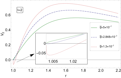
Qualitatively speaking, the dynamical instability 666One should avoid confusing this kind of instability with the ghost and Laplacian instabilities discussed in Tsujikawa21 . In fact, by following the formalism of Tsujikawa21 and using the Lagrangian represented by (3.16), it’s straightforward to exclude these two kinds of instabilities for the and cases. mentioned above could mainly be attributed to the features of the effective potential . As seen from Fig. 4, the effective potential can stay positive once is large enough. In contrast, a small may drag a part of to the negative regime. By following the formalism of Takahashi2013 ; Gannouji2022 , we notice that being negative on (or , although we abbreviated this part of the discussion since was observed to stay positive for all the reasonable ’s, e.g., those considered in Fig. 2) can introduce instability to our dynamical system. This explains the peculiar behaviors of shown in Fig. 2 and Fig. 3 777Notice that, although stays positive (at least for the physically allowed values of ’s), a general analysis to the PDEs tells us that the blowing-up feature of could be conveyed to Evans2010 , as now is acting as its source term [cf., Eq.(4.3)]. On the other hand, one should not forget that in fact carries the information of by definitions (III.2) and (IV.1).. Thus, although it sounds a little counter-intuitive, we conclude that a relatively large can guarantee the stability of our dynamical system 888Similar analysis to this kind of dynamical instability could be done for Kai2016 . It is also due to the negative sign of the corresponding effective potential (under certain choices of the coupling constant), that instability occurs. Nonetheless, different from our case, in there, a smaller coupling constant could erase such an instability., while on the other hand (as expected) enhancing the deviation between and , and vice versa.
Another interesting phenomenon is that, the instability mentioned above could be relaxed a little bit for a larger . As seen from Fig.5, for same , choosing a relatively larger could postpone the time of being blow-up for (what we observed here is different from that of Konoplya2008 ). That is, higher multipoles tend to be more stable.
It is worth mentioning here that, the ratio between and plays an important role in controlling the numerical stability during the calculations of . By defining , a Courant-like stability condition is given by (see, e.g., the §6.5 of Habermanb and LeVeque2007 )
| (4.9) |
where . Since the numerical values of and can be easily obtained, we can solve for the approximate valid region of from (4.9) for any specific . We then noticed that, for the case and a typical [viz., ], could guarantee the condition (4.9). This could be further confirmed by monitoring the behavior of solved with the varying . Indeed, we observed that the deformation of curves of shows a convergent behavior for [In contrast, the curve of resultant is sensitive to the choice of for , which reflects a numerical instability]. Notice that, such a convergent behavior also supports the validity of the individual values of our chosen and 999 To be specific, the emergence of such a convergent behavior means the reasonable variations of and won’t change our numerical results. Technically speaking, and are the most significant factors in our numerical method. Other software-related factors were found to have trivial influence on the numerical results, as long as we are working under a hing enough precision and accuracy (this is exactly what we did in practice). Therefore, by following some general protocols of judging a numerical method, we are able to exclude the numerical instabilities for our results. .
V Conclusions
In this paper, we investigated QNMs of odd-parity perturbations in Einstein-Æther theory. Specially, here we pay attention to a kind of wormhole-like backgrounds, described by (II.2). To find the corresponding QNMs, we first work in the isotropic coordinate and simplify the 2nd-order Lagrangian to Eq.(3.16) by following Tsujikawa21 . Then, the desired master equations in the Schwarzschild coordinate could be obtained in terms of a set of coupled PDEs [cf., Eqs.(4.3) and (4.4)], which depend only on the coupling constant (or equivalently, ), after setting from the requirement of no-ghost conditions Tsujikawa21 and constraints from observations [cf., (2.16)].
As has been mentioned in Sec. I, there are many different techniques in general for calculating QNMs. However, in reality, the FDM is identified as one of the most apt ways for our case. By mainly focusing on the mode (due to its physical significance Mag18 ; Shi2019 ; Ghosh2021 ; LVK2022 ), that set of PDEs are solved numerically with the help of the recursion formula (4.7). By varying the coupling constant , or equivalently, [cf., (II.2)], the corresponding solutions are shown in terms of vs. , and are exhibited in Figs. 2 and 3.
As shown in Sec. IV. B, we read off the features of , and their dependence on from Figs. 2 and 3. Specially, we found that choosing the physically allowed values of ’s [cf., (2.16)] will bring the dynamical system to a kind of instability (which is different from that found in Tsujikawa21 ), as observed from the panels (a)-(c) of Fig. 2. This phenomenon is actually consistent with the behaviors of the effective potentials [cf., Eq.(IV.1)], since a physically allowed value of will drag a part of the potential to the negative regime [cf., Fig. 4]. Therefore, we conclude that the background solutions described by (II.2) are not stable against the odd-parity perturbations and should be ruled out.
Acknowledgements
This work is supported by the National Key Research and Development Program of China under Grant No.2020YFC2201503, the National Natural Science Foundation of China under Grant No. 12275238, No. 11975203, No. 11675143, No. 12205254, the Zhejiang Provincial Natural Science Foundation of China under Grant No. LR21A050001 and LY20A050002, and the Fundamental Research Funds for the Provincial Universities of Zhejiang in China under Grant No. RF-A2019015.
Appendix A: Integral formulas for spherical harmonics
The spherical harmonics has the following integral features Zettili ; Kase:2018voo
| (A. 1) | |||
| (A. 2) | |||
| (A. 3) |
Appendix B: Expressions of
The coefficients that appear in Eq.(3.16) are given by
| (B. 1) |
Here, a prime in the superscript denotes the derivative with respect to .
Appendix C: Expressions of
The coefficients that appear in Eq.(IV.1) are given by
| (C. 1) |
Here, a prime in the superscript denotes the derivative with respect to .
Appendix D: The formulas for obtaining Schrödinger-like PDEs
The procedures for obtaining Eqs.(4.3) and (4.4) may not be that straightforward. To show it more clearly, here we introduce the formulas used in this part of calculations. Suppose we have a set of linearly coupled 2nd-order PDEs of the form
Let us introduce a set of new functions and a new variable by
| (D. 2) |
Then, choosing as
| (D. 3) |
we find that Eq.(Appendix D: The formulas for obtaining Schrödinger-like PDEs) can be written as a set of coupled Schrödinger-like PDEs
| (D. 4) |
where
| (D. 5) | |||||
and
| (D. 6) |
Here a prime denotes the derivative with respect to . In addition, a common choice of is . Notice that, since we were considering the case in deriving Eqs.(4.3) and (4.4), the corresponding and are happen to be identical under this condition.
References
- (1) B.P. Abbott, et al., [LIGO/Virgo Scientific Collaborations], Observation of Gravitational Waves from a Binary Black Hole Merger, Phys. Rev. Lett. 116, 061102 (2016).
- (2) B.P. Abbott, et al., [LIGO/Virgo Collaborations], GWTC-1: A Gravitational-Wave Transient Catalog of Compact Binary Mergers Observed by LIGO and Virgo during the First and Second Observing Runs, Phys. Rev. X9, 031040 (2019).
- (3) B.P. Abbott, et al., [LIGO/Virgo Collaborations], Open data from the first and second observing runs of Advanced LIGO and Advanced Virgo, SoftwareX, Volume 13, 100658 (2021).
- (4) B.P. Abbott, et al., [LIGO/Virgo Collaborations], GW190425: Observation of a Compact Binary Coalescence with Total Mass , ApJL 892 L3 (2020).
- (5) B.P. Abbott, et al., [LIGO/Virgo/KAGRA Collaborations], GWTC-3: Compact Binary Coalescences Observed by LIGO and Virgo During the Second Part of the Third Observing Run, arXiv:2111.03606v1 [gr-qc].
- (6) C. J. Moore, R. H. Cole and C. P. L. Berry, Gravitational-wave sensitivity curves, Class. Quantum. Grav. 32, 015014 (2015).
- (7) Y. Gong, J. Luo and B. Wang, “Concepts and status of Chinese space gravitational wave detection projects,” Nature Astron. 5, no.9, 881-889 (2021).
- (8) E. Berti, V. Cardoso and A. O. Starinets, Quasinormal modes of black holes and black branes, Class. Quantum. Grav. 26, 163001 (2009).
- (9) E. Berti, K. Yagi, H. Yang, N. Yunes, Extreme gravity tests with gravitational waves from compact binary coalescences: (II) ringdown, Gen. Relativ. Grav. 50, 49 (2018).
- (10) R. A. Konoplya, How to tell the shape of a wormhole by its quasinormal modes, Physics Letters B 784, 43–49 (2018).
- (11) S. H. Völkel and K. D. Kokkotas, Wormhole potentials and throats from quasi-normal modes, Class. Quantum Grav. 35, 105018 (2018).
- (12) J. Y. Kim, C. O. Lee and M.-I. Park, Quasinormal modes, Quasi-normal modes of a natural AdS wormhole in Einstein–Born–Infeld Gravity, Eur. Phys. J. C, 78:990 (2018).
- (13) E. Franzin, S. Liberati, J. Mazza, R. Dey and S. Chakraborty, Scalar perturbations around rotating regular black holes and wormholes: Quasinormal modes, ergoregion instability, and superradiance, Phys. Rev. D105, 124051 (2022).
- (14) E. Berti, K. Yagi, H. Yang, N. Yunes, Extreme gravity tests with gravitational waves from compact binary coalescences: (I) inspiral-merger, Gen. Relativ. Grav. 50, 46 (2018).
- (15) CE, https://cosmicexplorer.org/.
- (16) ET Steering Committee Editorial Team, ET design report update 2020, ET-0007A- 20 (2020); https://www.et-gw.eu/.
- (17) https://www.lisamission.org
- (18) S. Liu, Y. Hu, et al., Science with the TianQin observatory: Preliminary results on stellar-mass binary black holes, Phys. Rev. D101, 103027 (2020).
- (19) C.-F. Shi, et al., Science with the TianQin observatory: Preliminary results on testing the no-hair theorem with ringdown signals, Phys. Rev. D100, 044036 (2019).
- (20) W.-H. Ruan, Z.-K. Guo, R.-G. Cai, Y.-Z. Zhang, Taiji Program: Gravitational-Wave Sources, Int. J. Mod. Phys. A 35, No. 17, 2050075 (2020).
- (21) S. Kawamura, et al., Current status of space gravitational wave antenna DECIGO and B-DECIGO, arXiv:2006.13545.
- (22) S. Chandrasekhar, the mathematical theory of black holes, Oxford classic texts in the physical sciences (Oxford Press, Oxford, 1992).
- (23) S. Iyer, Black-hole normal modes: A WKB approach. II. Schwarzschild black holes, Phys. Rev. D35, 3632 (1987).
- (24) S. Detweiler, BLACK HOLES AND GRAVITATIONAL WAVES. III. THE RESONANT FREQUENCIES OF ROTATING HOLES, Astrophys. J. 239, 292-295 (1980).
- (25) E. Seidel and S. Iyer, Black-hole normal modes: A WKB approach. IV. Kerr black holes, Phys. Rev. D41, 2 (1990).
- (26) B. F. Schutz and C. M. Will, BLACK HOLE NORMAL MODES: A SEMIANALYTIC APPROACH, Astrophys. J. 291, L33-L36 (1985).
- (27) S. Iyer and C. M. Will, Black-hole normal modes: A WKB approach. I. Foundations and application of a higher-order WKB analysis of potential-barrier scattering, Phys. Rev. D35, 12, 3621-3631 (1987).
- (28) R. A. Konoplya, Quasinormal behavior of the D-dimensional Schwarzschild black hole and the higher order WKB approach, Phys. Rev. D68, 024018 (2003).
- (29) J. Matyjasek and M. Opala, Quasinormal modes of black holes: The improved semianalytic approach, Phys. Rev. D96, 024011 (2017).
- (30) X. Li and S.-P. Zhao, Quasinormal modes of a scalar and an electromagnetic field in Finslerian-Schwarzschild spacetime, Phys. Rev. D101, 124012 (2020).
- (31) E. W. Leaver, An analytic representation for the quasi-normal modes of Kerr black holes, Proc. R. Soc. Lond. A. 402, 285-298 (1985).
- (32) S. Chandrasekhar, F. R. S., and S. Detweiler, The quasi-normal modes of the Schwarzschild black hole, Proc. R. Soc. Lond. A. 344, 411-452 (1975).
- (33) D. D. Doneva, S. S. Yazadjiev, K. D. Kokkotas, and I. Zh. Stefanov, Quasinormal modes, bifurcations, and nonuniqueness of charged scalar-tensor black holes, Phys. Rev. D82, 064030 (2010).
- (34) K. Lin and W.-L. Qian, A matrix method for quasinormal modes: Schwarzschild black holes in asymptotically flat and (anti-) de Sitter spacetimes, Class. Quantum Grav. 34, 095004 (2017).
- (35) R. A. Konoplya and A. Zhidenko, Quasinormal modes of black holes: From astrophysics to string theory, Rev. Mod. Phys. 83, 793 (2011).
- (36) C. Gundlach, R. H. Price and J. Pullin, Late-time behavior of stellar collapse and explosions. I. Linearized perturbations, Phys. Rev. D49, 883 (1994).
- (37) B. Wang, C.-Y. Lin and C. Molina, Quasinormal behavior of massless scalar field perturbation in Reissner-Nordström anti-de Sitter spacetimes, Phys. Rev. D70, 064025 (2004).
- (38) O. J. Tattersall and P. G. Ferreira, Forecasts for low spin black hole spectroscopy in Horndeski gravity, Phys. Rev. D99, 104082 (2019).
- (39) R.A. Konoplya, A. Zhidenko, Gravitational spectrum of black holes in the Einstein-Aether theory, Phys. Lett. B648, 236 (2007).
- (40) H. Yang, D. A. Nichols, F. Zhang, et al., Quasinormal-mode spectrum of Kerr black holes and its geometric interpretation, Phys. Rev. D86, 104006 (2012).
- (41) T. Jacobson, Einstein-ther gravity: a status report, Proc. Sci., QG-PH (2007) 020 [arXiv:0801.1547v2]
- (42) J. Oost, S. Mukohyama and A. Wang, Constraints on -theory after GW170817, Phys. Rev. D97, 124023 (2018).
- (43) S. Tsujikawa, C. Zhang, X. Zhao and A. Wang, Odd-parity stability of black holes in Einstein-Aether gravity, Phys. Rev. D104, 064024 (2021).
- (44) O. Sarbach, E. Barausse, and J.A Preciado-López, Well-posed Cauchy formulation for Einstein-ther theory, Class. Quantum Grav. 36 (2019) 165007.
- (45) D. Garfinkle and T. Jacobson, A Positive-Energy Theorem for Einstein-Aether and Hořava Gravity, Phys. Rev. Lett. 107, 191102 (2011).
- (46) T. Clifton, P.G. Ferreira, A. Padilla, C. Skordis, Modified Gravity and Cosmology, Phys. Reports 513, 1 (2012).
- (47) D. Langlois, Dark energy and modified gravity in degenerate higher-order scalar-tensor (DHOST) theories: A review, Inter. J. Mod. Phys. D28, 1942006 (2019).
- (48) A. Bourgoin, et al., Constraining velocity-dependent Lorentz and CPT violations using lunar laser ranging, Phys. Rev. D103, 064055 (2021).
- (49) H. Pihan-le Bars, etal., New Test of Lorentz Invariance Using the MICROSCOPE Space Mission, Phys. Rev. Lett. 123, 231102 (2019).
- (50) C.G. Shao, et al., Combined Search for a Lorentz-Violating Force in Short-Range Gravity Varying as the Inverse Sixth Power of Distance, Phys. Rev. Lett. 122, 011102 (2019).
- (51) A. Bourgoin, C. Le Poncin-Lafitte, A. Hees, S. Bouquillon, G. Francou, and M.-C. Angonin, Lorentz Symmetry Violations from Matter-Gravity Couplings with Lunar Laser Ranging, Phys. Rev. Lett. 119, 201102 (2017).
- (52) N.A. Flowers, C. Goodge, and J.D. Tasson, Superconducting-Gravimeter Tests of Local Lorentz Invariance, Phys. Rev. Lett. 119, 201101 (2017).
- (53) A. Kostelecky and N. Russell, Data tables for Lorentz and CPT violation, Rev. Mod. Phys. 83 11 (2011) [arXiv:0801.0287v15, January 2022 Edition].
- (54) J. Collins, A. Perez, D. Sudarsky, L. Urrutia, and H. Vucetich, Lorentz invariance and quantum gravity: an additional fine-tuning problem?, Phys. Rev. Lett. 93 (2004) 191301.
- (55) D. Mattingly, Modern Tests of Lorentz Invariance, Living Rev. Relativity, 8, 5 (2005).
- (56) S. Liberati, Tests of Lorentz invariance: a 2013 update, Class. Quantum Grav. 30, 133001 (2013).
- (57) M. Pospelov and C. Tamarit, Lifshitz-sector mediated SUSY breaking, J. High Energy Phys. 01 (2014) 048.
- (58) A. Wang, Hořava gravity at a Lifshitz point: A progress report, Inter. J. Mod. Phys. D26, 1730014 (2017).
- (59) T. Jacobson and D. Mattingly, Einstein-aether waves, Phys. Rev. D70, 024003 (2004).
- (60) J. W. Elliott, G. D. Moore and H. Stoica, Constraining the New Aether: Gravitational Cherenkov Radiation, JHEP 0508, 066 (2005).
- (61) J. Calderón Bustillo, P.D. Lasky, and E. Thrane, Black-hole spectroscopy, the no-hair theorem, and GW150914: Kerr versus Occam, Phys. Rev. D103, 024041 (2021).
- (62) R. Abbott, etal. [The LIGO and Virgo Collaborations], Tests of general relativity with binary black holes from the second LIGO-Virgo gravitational-wave transient catalog, Phys. Rev. D103, 122002 (2021).
- (63) X. J. Forteza, S. Bhagwat, P. Pani, and V. Ferrari, Spectroscopy of binary black hole ringdown using overtones and angular modes, Phys. Rev. D102, 044053 (2020).
- (64) S. Bhagwat, X. J. Forteza, P. Pani, and V. Ferrari, Ringdown overtones, black hole spectroscopy, and no-hair theorem tests, Phys. Rev. D101, 044033 (2020).
- (65) M. Giesler, M. Isi, M. Scheel, and S. Teukolsky, Black Hole Ringdown: The Importance of Overtones, Phys. Rev. X 9, 041060 (2019).
- (66) M. Isi, M. Giesler, W. M. Farr, M. A. Scheel, and S. A. Teukolsky,Testing the No-Hair Theorem with GW150914, Phys. Rev. Lett. 123, 111102 (2019).
- (67) G. Carullo, W. Del Pozzo, and J. Veitch, Observational black hole spectroscopy: A time-domain multimode analysis of GW150914, Phys. Rev. D 99, 123029 (2019).
- (68) C.D. Capano and A.H. Nitz, Binary black hole spectroscopy: A no-hair test of GW190814 and GW190412, Phys. Rev. D102, 124070 (2020).
- (69) I. Ota and C. Chirenti, Overtones or higher harmonics? Prospects for testing the no-hair theorem with gravitational wave detections, Phys. Rev. D101, 104005 (2020).
- (70) F.H. Shaik, J. Lange, S.E. Field, R. O’Shaughnessy, V. Varma, L.E. Kidder, H.P. Pfeiffer, and D. Wysocki, Impact of subdominant modes on the interpretation of gravitational-wave signals from heavy binary black hole systems, Phys. Rev. D101, 124054 (2020).
- (71) N. Uchikata, T. Narikawa, K. Sakai, H. Takahashi, and Hiroyuki Nakano, Black hole spectroscopy for KAGRA future prospect in O5, Phys. Rev. D102, 024007 (2020).
- (72) S. Bhagwat, M. Cabero, C.D. Capano, B. Krishnan, and D.A. Brown, Detectability of the subdominant mode in a binary black hole ringdown, Phys. Rev. D102, 024023 (2020).
- (73) M. Cabero, J. Westerweck, C.D. Capano, S. Kumar, A.B. Nielsen, and B. Krishnan, Black hole spectroscopy in the next decade, Phys. Rev. D101, 064044 (2020).
- (74) A. Maselli, P. Pani, L. Gualtieri, and E. Berti, Parametrized ringdown spin expansion coefficients: A data-analysis framework for black-hole spectroscopy with multiple events, Phys. Rev. D101, 024043 (2020).
- (75) T. Islam, A.K. Mehta, A. Ghosh, V. Varma, P. Ajith, and B.S. Sathyaprakash, Testing the no-hair nature of binary black holes using the consistency of multipolar gravitational radiation, Phys. Rev. D101, 024032 (2020).
- (76) B. P. Abbott, et al., [LIGO/Virgo/KAGRA Collaborations], Tests of General Relativity with GWTC-3, arXiv:2112.06861v1 [gr-qc].
- (77) S. M. Carroll and E. A. Lim, Lorentz-violating vector fields slow the universe down, Phys. Rev. D70, 123525 (2004).
- (78) C. Zhang, X. Zhao, K. Lin, S.-J. Zhang, W. Zhao and A.-Z. Wang, Spherically symmetric static black holes in Einstein-aether theory, Phys. Rev. D102, 064043 (2020).
- (79) T. Gupta, M. Herrero-Valea, D. Blas, E. Barausse, N. Cornish, K. Yagi, N. Yunes, New binary pulsar constraints on Einstein-æther theory after GW170817, Class. Quantum Grav. 38, 195003 (2021).
- (80) J. Müller, J.G. Williams and S.G. Turyshev, Lunar laser ranging contributions to relativity and geodesy, Astrophys. Space Sci. Libr. 349 (2008) 457.
- (81) S. Weinberg, Gravitation and Cosmology: Principles and Applications of the General Theory of Relativity (John Wiley & Sons, Inc., USA, 1972).
- (82) J. Oost, S. Mukohyama and A. Wang, A. Spherically Symmetric Exact Vacuum Solutions in Einstein-Aether Theory. Universe, 7, 272 (2021).
- (83) J. E. Thompson, H. Chen and B. F. Whiting, Gauge invariant perturbations of the Schwarzschild spacetime, Class. Quantum Grav. 34 174001 (2017).
- (84) T. Regge and J. A. Wheeler, Stability of a Schwarzschild Singularity, Phys. Rev. 108, 4 (1957).
- (85) R. d’ Inverno, Introducing Einstein’s Relativity (Oxford University Press, New York, 2000).
- (86) G. B. Arfken, H. J. Weber and F. E. Harris Mathematical Methods for Physicists (7th ed) (Elsevier Inc, UK, 2013).
- (87) J. R. Taylor, Classical mechanics (University Science Books, USA, 2005).
- (88) Richard Haberman, APPLIED PARTIAL DIFFERENTIAL EQUATIONS: with Fourier Series and Boundary Value Problems (5th ed.) (Pearson Education, Inc., One Lake Street, New Jersey 07458, USA, 2013).
- (89) K. Lin, W. Qian and A. B. Pavan, Scalar quasinormal modes of anti–de Sitter static spacetime in Horava-Lifshitz gravity with U(1) symmetry, Phys. Rev. D94, 064050 (2016).
- (90) M. Maggiore, Gravitational Waves Volume 2: Astrophysics and Cosmology (Oxford University Press, New York, 2018).
- (91) A. Ghosh, R. Brito and A. Buonanno, Constraints on quasinormal-mode frequencies with LIGO-Virgo binary–black-hole observations, Phys. Rev. D103, 124041 (2021).
- (92) M. A. Cuyubamba, R. A. Konoplya and A. Zhidenko, No stable wormholes in Einstein-dilaton-Gauss-Bonnet theory, Phys. Rev. D98, 044040 (2018).
- (93) R. A. Konoplya and A. Zhidenko, (In)stability of D-dimensional black holes in Gauss-Bonnet theory, Phys. Rev. D77, 104004 (2008).
- (94) T. Takahashi, Instability of charged Lovelock black holes: Vector perturbations and scalar perturbations, Prog. Theor. Exp. Phys, 013E02 (2013).
- (95) R. Gannouji and Y. R. Baez, Stability of generalized Einstein-Maxwell-scalar black holes, JHEP 02, 020 (2022).
- (96) L.C. Evans, Partial Differential Equations (2nd ed.) (American Mathematical Society, USA, 2010).
- (97) Randall J. LeVeque, Finite Difference Methods for Ordinary and Partial Differential Equations: Steady-State and Time-Dependent Problems (Society for Industrial and Applied Mathematics, USA, 2007).
- (98) N. Zettili, Quantum Mechanics: Concepts and Applications (2nd ed.) (CPI Antony Rowe Ltd, Chippenham, Wiltshire, UK, 2009).
- (99) R. Kase, M. Minamitsuji, S. Tsujikawa and Y. L. Zhang, Black hole perturbations in vector-tensor theories: The odd-mode analysis, JCAP 02, 048 (2018).