Stationary Two-State System in Optics using Layered Materials

Abstract

When electrodynamics is quantized in a situation where electrons are confined to a flat surface, as in the case of graphene, one of the Maxwell’s equations emerges as a local component of the Hamiltonian. We demonstrate that, owing to the residual gauge invariance for the local Hamiltonian, nontrivial constraints on physical states arise. We construct two stationary quantum states with a zero energy expectation value: one replicates the scattering and absorption of light, a phenomenon familiar in classical optics, while the other is more fundamentally associated with photon creation. According to the Hamiltonian, these two states are inseparable, forming a two-state system. However, there exists a specific number of surfaces for which the two states become decoupled. This number is $2/\pi\alpha$, where $\pi\alpha$ is the absorption probability of a single surface. To explore the physics that can emerge in such decoupled cases, we investigate certain perturbations that can influence a two-state system based on symmetry considerations, utilizing concepts such as parity, axial (pseudo) gauge fields, and surface deformation.

Two-state systems represent the simplest cases that exhibit the essential features of quantum physics. Examples include spin-$1/2$, the two base states for the ammonia molecule, (clockwise and counterclockwise) persistent currents of superconducting qubit, and the hydrogen molecular ion. [1, 2] In optical science, the two-state polarization of the radiation field plays a fundamental role in uncovering the laws of physics, such as the non-cloning theorem, [3] serving as a source of quantum entanglement, [4, 5, 6, 7] and contributing to modern optical transmission technology, allowing for the simultaneous transmission of double the amount of information. Recently, the two-state coherent phase of a pulsed field has been related to an artificial spin. [8, 9] There may be more two-state systems in optics beyond these examples. Even when a system appears to have many degrees of freedom, it is sometimes apparent that, from a certain perspective, only two crucial states play an essential role in the mechanism of the phenomenon under investigation. [10, 11, 12, 13] In this paper, we employ quantum electrodynamics [14] to illustrate the existence of two stationary quantum states in optics involving layered materials. Our formulation reveals that the appearance of these two states is intricately connected to gauge invariance, and the origin of the two-state degree of freedom is inherently linked to the chiral nature of photons, specifically the right- and left-going components. We show that the antisymmetric combinations of counter-propagating photons are connected to the axial gauge field, suggesting a potential link to the geometrical deformation of layered materials and the Raman effect.

The space is divided into two regions, $x<0$ (left) and $x>0$ (right), by an absorbing surface located at $x=0$. Some fraction of a continuum incident light coming from $x=-\infty$ is absorbed only by the surface where the electronic current ${\bf j}$ exists, and the remaining is either reflected back to $x=-\infty$ or transmitted forward to $x=+\infty$. In the classical theory of optics, the reflection and transmission coefficients are derived from Ampére’s circuital law, given by $c^{2}\nabla\times{\bf B}=\frac{\bf j}{\epsilon_{0}}+\dot{\bf E}$. Integrating this equation with respect to an infinitesimal element around the surface, the magnetic field experiences a discontinuity at the surface, expressed as $c^{2}\{B_{y}(0_{+})-B_{y}(0_{-})\}=\int_{0_{-}}^{0_{+}}\frac{j_{z}}{\epsilon_{0}}dx$, due to the localization of the current $j_{z}=J_{z}\delta(x)$ about the surface. [15, 16] Meanwhile, the electric field $E_{z}$ remains continuous at the surface, and the last term of Ampére’s circuital law vanishes upon integration. Since the magnetic field is expressed in terms of the radiation gauge field by $B_{y}=-\partial_{x}A_{z}$, we obtain the boundary condition

$$\partial_{x}A_{z}|_{x=0_{+}}-\partial_{x}A_{z}|_{x=0_{-}}+\frac{J_{z}}{\epsilon_{0}c^{2}}=0,$$ (1)

showing that the first derivative of $A_{z}(x)$ is discontinuous at the surface, meanwhile, $A_{z}(x)$ must be continuous. Equation (1) is also derived as a characteristic of stationary states within the Poynting theory. [1] The continuity equation is expressed as $E_{z}j_{z}+\partial_{x}S_{x}+\dot{U}_{em}=0$, where $S_{x}=-\epsilon_{0}c^{2}E_{z}B_{y}$ represents the Poynting vector, and $U_{em}=\frac{\epsilon_{0}}{2}(E_{z}^{2}+c^{2}B_{y}^{2})$ is the energy density of the electromagnetic field. In the context of stationary states, $\dot{U}_{em}=0$, allowing us to reproduce Eq. (1) by integrating $E_{z}j_{z}+\partial_{x}S_{x}=0$ with respect to an infinitesimal element around $x=0$. Now, in quantum field theory, $A_{z}(x)$ as well as $J_{z}$ is a field operator consisting of particle creation and annihilation operators.

It is possible to show that Eq. (1) appears as a part of Hamiltonian and is related to the gauge invariance in the fundamental level. For the photon’s Hamiltonian of

$$H_{ph}=\frac{\epsilon_{0}}{2}\int_{-\infty}^{+\infty}dx\left\{\dot{A}_{z}(x)^{2}+c^{2}(\partial_{x}A_{z}(x))^{2}\right\},$$ (2)

the integral may be divided into a left region, right region, and the surface $[0_{-},0_{+}]$. Then, the Hamiltonian of the radiation field at the surface is given by $\epsilon_{0}c^{2}A_{z}(x)\partial_{x}A_{z}(x)|_{0_{-}}^{0_{+}}$. By combining it with the gauge coupling of the interaction Hamiltonian, $H_{int}=A_{z}(0)J_{z}$, we obtain the Hamiltonian at the surface $H_{ph}|_{x=0}+H_{int}(\equiv H_{local})$ as

$$\epsilon_{0}c^{2}A_{z}(0)\left\{\partial_{x}A_{z}(x)|_{x=0_{+}}-\partial_{x}A_{z}(x)|_{x=0_{-}}+\frac{J_{z}}{\epsilon_{0}c^{2}}\right\}.$$ (3)

To simplify the notation, we use ${\cal B}$ to denote the operator of the boundary condition, ${\cal B}\equiv\partial_{x}A_{z}(x)|_{x=0_{+}}-\partial_{x}A_{z}(x)|_{x=0_{-}}+\frac{J_{z}}{\epsilon_{0}c^{2}}$, and the local Hamiltonian is rewritten as

$$H_{local}=\epsilon_{0}c^{2}A_{z}(0){\cal B}.$$ (4)

The Hamiltonian must be invariant with respect to a residual gauge transformation, given by $A_{z}(0)\to A_{z}(0)+\partial_{z}\lambda(x,z)|_{x=0}$, where $\lambda(x,z)=Cz$ satisfies $\partial^{2}_{z}\lambda(x,z)=0$. However, the local Hamiltonian changes under such a residual gauge transformation as $H_{local}\to H_{local}+\epsilon_{0}c^{2}C{\cal B}$. Thus, to ensure that a residual gauge transformation does not alter the energy of physical states, any physical state $|\Phi\rangle$ must satisfy the condition $\langle\Phi|{\cal B}|\Phi\rangle=0$. Instead of stating that Eq. (1) is satisfied as the expectation value (Ehrenfest’s theorem), Eq. (1) is satisfied as a consequence of the residual gauge symmetry. [17] Additionally, any physical state should not overlap with a state generated by acting the vacuum with ${\cal B}$, i.e., $\langle\Phi|{\cal B}\left(|0\rangle\otimes|vac\rangle\right)=0$, where the ground state of the photon (matter) is expressed by $|0\rangle$ ($|vac\rangle$). Failure to meet this condition could allow a residual gauge transformation to introduce an arbitrary amount of energy, which is a scenario not observed in nature. We note that the result of the Poynting theory, $E_{z}{\cal B}=0$, can be derived from $\dot{H}_{local}=0$ and $\dot{\cal B}=0$, because $E_{z}=-\dot{A}_{z}$.

We will show that the Hilbert space holds two quantum states denoted by $|\Phi_{a}\rangle$ and $|\Phi_{b}\rangle$. Each state is not single quantum but a specific combination of light and matter quanta. The former reproduces scattering and absorption of light by matter which is consistent with the classical description of optics, and the latter is more fundamentally related to the photon creation or light emission. We use the Schrödinger picture (representation), [2, 14] and the operators are time-independent. Moreover, the state vectors we construct are stationary states with zero-energy of the local Hamiltonian, the variable of time is concealed. The gauge field operator is a sum of right- and left-moving components as $A_{z}(x)=A_{R}(x)+A_{L}(x)$. The electric field operator is denoted by $E_{z}(x)$ which forms canonical equal-time commutation relations with $A_{z}(x)$, such as $\left[A_{z}(x),E_{z}(x^{\prime})\right]=-i\frac{\hbar c}{\epsilon_{0}}\delta(x-x^{\prime})$, $\left[A_{R}(x),E_{R}(x^{\prime})\right]=-i\frac{\hbar c}{2\epsilon_{0}}\delta(x-x^{\prime})$, and $\left[A^{+}(x),E^{-}(x^{\prime})\right]=-i\frac{\hbar c}{2\epsilon_{0}}\delta(x-x^{\prime})$, where $-$ and $+$ of the superscript stands for the annihilation and creation part of the field operators, respectively. Note that $A_{z}(x)$ commutes with $B_{y}(x^{\prime})$ and so with ${\cal B}$. However, each component satisfies $[\partial_{x}A_{R}(x),A_{R}(x^{\prime})]=+i\frac{\hbar}{2\epsilon_{0}}\delta(x-x^{\prime})$ and $[\partial_{x}A_{L}(x),A_{L}(x^{\prime})]=-i\frac{\hbar}{2\epsilon_{0}}\delta(x-x^{\prime})$, which are canceled in $[B_{y}(x),A_{z}(x^{\prime})]=0$.

First, we define an entangled state that is a superposition of right- and left-going photons counter-propagating along the $x$-axis. The spatially uniformity of the light state is perturbed by the absorbing surface as $|a\rangle=N_{a}\int_{-\infty}^{+\infty}a(x)dx|0\rangle$ and

$$a(x)=\left[\theta(-x)+t\theta(x)\right]e^{i\frac{\omega}{c}x}A_{R}(x)+r\theta(-x)e^{-i\frac{\omega}{c}x}A_{L}(x).$$ (5)

Here, $t$ ($r$) is the transmission (reflection) coefficient, $N_{a}$ is a normalization constant of the state $|a\rangle$ (space is taken to be infinity), and $\theta(x)$ is the step function; $\theta(x)=1$ for $x>0$ and vanishes otherwise. We show below that the following quantum state reproduces the result obtained in classical optics, [18]

$$|\Phi_{a}\rangle\equiv|a\rangle\otimes|vac\rangle+\frac{\langle 0|E_{z}(0)|a\rangle}{g}|0\rangle\otimes J_{z}|vac\rangle.$$ (6)

Since the electric field is continuous at the surface (as we see below), we can also take either $x=0_{+}$ or $0_{-}$ for the argument of $E_{z}$. A constant $g$ is introduced for dimensional consistency whose value is not of particular importance here. The classical physics is reproduced by replacing $|a\rangle$ with a coherent state $|A\rangle=N_{A}e^{i\int_{-\infty}^{+\infty}a(x)dx}|0\rangle$.

To specify $|\Phi_{a}\rangle$ uniquely, we use two physical conditions. First condition is the continuity of the electric field $\langle 0|E_{z}(0_{-})|a\rangle=\langle 0|E_{z}(0_{+})|a\rangle$ giving $1+r=t$. Second is the necessary condition with respect to a physical state,

$$\langle 0|\otimes\langle vac|{\cal B}|\Phi_{a}\rangle=0.$$ (7)

Using commutation relations, we obtain from Eq. (7)

$$i\frac{\hbar}{2\epsilon_{0}}t-i\frac{\hbar}{2\epsilon_{0}}(1-r)+\frac{\sigma g}{\epsilon_{0}c^{2}}i\frac{1}{g}\frac{\hbar c}{2\epsilon_{0}}t=0.$$ (8)

We note that $\langle vac|J_{z}J_{z}|vac\rangle=g\sigma$, where $\sigma$ is dynamical conductivity (or vacuum polarization). In the case of graphene, the dynamical conductivity is given by $\sigma=\pi\alpha\epsilon_{0}c$, where $\alpha$ is the fine-structure constant (the absorption probability is $\pi\alpha\sim$ 2.3 percent). [19, 20, 21] Thus, these two conditions lead to $t=\frac{2}{2+\pi\alpha}$ and $r=\frac{-\pi\alpha}{2+\pi\alpha}$. Moreover, we obtain $\langle\Phi_{a}|H_{local}|\Phi_{a}\rangle=0$ which also reproduces the energy (or probability) conservation given by Poynting vector, $1-r^{2}-t^{2}=\pi\alpha t^{2}(\equiv A_{abs})$. [15, 16] To calculate $\langle a|A_{z}(0_{+})$, we take care that two-point correlation function such as $\langle 0|[A_{z}(x+\varepsilon),A_{z}(x)]|0\rangle$ has an anomalous commutator part when $\varepsilon$ is tiny (the length scale of wave function spreading). It is actually defined by $\lim_{\varepsilon\to 0}\langle 0|[(A_{R}(x+\varepsilon)+A_{L}(x-\varepsilon)),A_{z}(x)]|0\rangle$ which gives $\lim_{\varepsilon\to 0}\varepsilon\langle 0|[\partial_{x}A_{R}(x)-\partial_{x}A_{L}(x),A_{z}(x)]|0\rangle=\lim_{\varepsilon\to 0}\varepsilon\frac{i\hbar}{\epsilon_{0}}\delta(0)$.

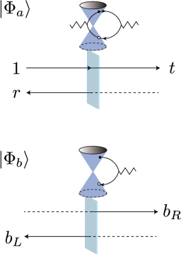
Figure 1: Schematic of the two-state system: It consists of $|\Psi_{a}\rangle$ and $|\Psi_{b}\rangle$, having a zero energy expectation value of $H_{local}$ due to the residual gauge symmtry. (Above) The arrow with “1” from left to right expresses the incident light ray, which is reflected or transmitted by a thin film (graphene). The dashed line represents the zero photon state. (Below) The state of light emission from the excited state is symmetrical in left and right directions. Only the off-diagonal matrix element of $H_{local}$, $\langle\Phi_{b}|H_{local}|\Phi_{a}\rangle$, is non-zero and proportional to $b_{R}^{*}t+b_{L}^{*}r$. The states of graphene are represented by the electron-hole pairs ($\bullet$ and $\circ$) in the Dirac cone (zigzag line denotes light). The electron-hole pairs in $|\Psi_{a}\rangle$ are virtual states of photons, while those in $|\Psi_{b}\rangle$ are real states that are constantly supplied by $|\Psi_{a}\rangle$.

Next we construct the other state vector,

$$|\Phi_{b}\rangle\equiv|b\rangle\otimes|vac\rangle+\frac{\langle 0|E_{z}(0)|a\rangle}{g}|0\rangle\otimes|exc\rangle,$$ (9)

where $|b\rangle=N_{a}\int_{-\infty}^{+\infty}b(x)dx|0\rangle$ and $b(x)=b_{R}\theta(x)e^{i\frac{\omega}{c}x}A_{R}(x)+b_{L}\theta(-x)e^{-i\frac{\omega}{c}x}A_{L}(x)$. It represents light emission from the surface. The presence of $\langle 0|E_{z}(0)|a\rangle$ on the last term shows that the emission is the spontaneous one (stimulated one when $|a\rangle\to|A\rangle$). The state vector of the matter $|exc\rangle$ denotes the excited state. This state is specified primarily by $J_{z}^{-}|exc\rangle=gF|vac\rangle$. In the same way as $|\Phi_{a}\rangle$, the continuity of the electric field with respect to $|b\rangle$, $\langle 0|E_{z}(0_{+})|b\rangle=\langle 0|E_{z}(0_{-})|b\rangle$, and the physical state condition $\langle 0|\otimes\langle vac|{\cal B}|\Phi_{b}\rangle=0$ are sufficient to obtain that $b_{R}=b_{L}(\equiv b)$ and

$$b=-\frac{F}{2\epsilon_{0}c}t.$$ (10)

This state automatically satisfies $\langle\Phi_{b}|H_{local}|\Phi_{b}\rangle=0$. Thus, we found that absorption means the two state-vectors and that the strength of emitted light depends on the electric field at the graphene layer ($t$).

Since $J_{z}^{+}J_{z}^{-}$ contains the number operator of electron-hole pairs $N_{eh}$, the expression $g^{2}|F|^{2}=g\sigma\langle exc|N_{eh}|exc\rangle$ is derived, representing the proportionality to the absorbed photon energy. The magnitude of $F$ is expressed as $|F|\propto\sqrt{A_{abs}}$, with the sign of $F$ depending on the specific characteristics of the matter system. [22, 23, 24] It’s worth noting that $|F|$ is influenced by the surrounding environment. For example, substrates supporting graphene can change the Fermi energy due to (unintentional) charge doping, affecting the nature of relaxations through Coulomb interactions,  known as impact excitations. [26] On the other hand, when graphene is suspended in the air, lattice vibrations do not decay into substrates, potentially reducing the relative significance of the paths from the excited states to light emission. To address these complexities, it is advisable to treat the effective magnitude of relaxations as a branching ratio ${\cal B}$, leading to the expression $|F|=\epsilon_{0}c\sqrt{2{\cal B}A_{abs}}$ or $|b|=\sqrt{({\cal B}/2)A_{abs}}|t|$. Physically, a large value of ${\cal B}$ implies that the excited states exhibit prolonged lifetimes, maintaining pathways for relaxation toward light emission.

Though the zero-energy conditions $\langle\Phi_{a}|H_{local}|\Phi_{a}\rangle=0$ and $\langle\Phi_{b}|H_{local}|\Phi_{b}\rangle=0$ are both satisfied, the off-diagonal element $\langle\Phi_{b}|H_{local}|\Phi_{a}\rangle$ is generally non-zero as

$$\langle\Phi_{b}|H_{local}|\Phi_{a}\rangle=\epsilon_{0}|E_{in}|^{2}\varepsilon b^{*}(t+r),$$ (12)

and therefore the two states evolve inseparably by the Hamiltonian. We shall introduce two states written as $|\Phi_{\theta}^{\pm}\rangle=|\Phi_{a}\rangle\pm e^{i\theta}|\Phi_{b}\rangle$, where the relative phase $\theta$ is determined so that these states are decoupled; $\langle\Phi^{+}_{\theta}|H_{local}|\Phi^{-}_{\theta}\rangle=0$ or ${\rm Im}[e^{i\theta}(t+r)^{*}b]=0$. Thus, $e^{i\theta}=\pm\frac{t+r}{|t+r|}\frac{b^{*}}{|b|}$. Then, their energy expectation values become non-zero as $\langle\Phi_{\theta}^{\pm}|H_{local}|\Phi_{\theta}^{\pm}\rangle=\pm 2(\epsilon_{0}|E_{in}|^{2}\varepsilon){\rm Re}[b^{*}(t+r)]$. An analogy to the electron spin is useful in understanding the physics. Suppose we have up and down spin states, $|\uparrow\rangle$ and $|\downarrow\rangle$, which are the eigenstates of $\sigma_{z}$. Let us assume that each spin state is in a magnetic field along the $y$-axis. The energy expectation value vanishes. Now, $|\Phi_{\theta}^{\pm}\rangle$ corresponds to $|\pm\rangle\equiv(|\uparrow\rangle\pm e^{i\theta}|\downarrow\rangle)/\sqrt{2}$. When $\theta$ is determined so that $\langle+|\sigma_{y}|-\rangle=0$, we have $\langle\pm|\sigma_{y}|\pm\rangle=\pm 1$. Note that the general expression of $H_{local}$ in terms of the spin is $H_{spin}=a_{+}\sigma_{+}+a_{-}\sigma_{-}$, where $\sigma_{\pm}=\sigma_{x}\pm i\sigma_{y}$ is the ladder operators and $a_{\pm}$ is the amplitudes. It satisfies $\langle\uparrow|H_{spin}|\uparrow\rangle=0$ and $\langle\downarrow|H_{spin}|\downarrow\rangle=0$.

Because the reflection coefficient is calculated by $\langle 0|E_{L}(-\infty)|\Phi^{\pm}_{\theta}\rangle$, $|\Phi_{b}\rangle$ appears as a correction to the reflection coefficient, and there are two possibilities of the correct reflection coefficient as

$$r\pm e^{i\theta}b=r\pm\left(\frac{t+r}{|t+r|}\right)|b|.$$ (13)

When the lower energy state $|\Phi^{-}_{\theta}\rangle$ is realized, the actual reflection is given by minus sign. Recently, we have applied a slight extension of this reflection formula to elucidate experiments conducted on multilayer graphene placed on substrates. [24] Our findings indicate that for visible range, substrates play a significant role in stabilizing $|\Phi^{-}_{\theta}\rangle$.

Due to absorption, the two states slightly overlap, i.e., $\langle\Phi_{b}|\Phi_{a}\rangle\neq 0$, and a simple interpretation of a two-state system is difficult to be applied. Apparently, from the reflected (or transmitted) light we will observe, the signal is inseparable between $|\Phi_{a}\rangle$ and $|\Phi_{b}\rangle$. If the two states were truly indistinguishable from each other, the situation is something like an electron spin in the absence of a magnetic field, and we need to face the issue of control. However, at least when $t+r=0$ is satisfied, $\langle\Phi_{b}|H_{local}|\Phi_{a}\rangle$ vanishes. Then, we define new base states, $|\Phi_{A}\rangle=|\Phi_{a}\rangle$ and $|\Phi_{B}\rangle=|\Phi_{b}\rangle-|\Phi_{a}\rangle\langle\Phi_{a}|\Phi_{b}\rangle$, which become orthogonal and are not mixed by the local Hamiltonian. Such an interesting situation is indeed possible to realize for multilayer graphene. [15] Let the layer number is $N$. The corresponding transmission and reflection coefficients are given by the replacement $\pi\alpha\to N\pi\alpha$ in $t$ and $r$. Thus, $t+r=0$ when $N=2/\pi\alpha$. Quite recently, we found also that one can access $|\Phi_{b}\rangle$ by suppressing the contribution of $|\Phi_{a}\rangle$ to the reflection ($r\sim 0$) using multilayer graphene (about 20 layers) and destructive interface effect of SiO₂/Si substrates. [24]

Perturbations should be incorporated into $H_{local}$, as they have the potential to disrupt stabilization and counteract corrections through interference. These perturbations arise from lattice vibrations and electron-phonon interactions, particularly in relation to the Raman effect. In this context, we examine some of these perturbations on symmetry considerations. Firstly, we observe that $H_{local}$ remains invariant under parity, as the fields transform according to $A_{z}(x)\to-A_{z}(-x),B_{y}(x)\to B_{y}(-x)$, and $J_{z}\to-J_{z}$. Let us introduce the axial (pseudo) gauge field $A^{ax}_{z}\equiv A_{R}-A_{L}$, which is even under parity as $A^{ax}_{z}(x)\to A^{ax}_{z}(-x)$. [27] This is in contrast to the polar one $A_{z}=A_{R}+A_{L}$. Since $A_{z}(x)$ and $A_{z}^{ax}(x)$ are regarded as the bonding and anti-bonding orbitals of counter-propagating photons, $A_{z}^{ax}(x)$ is useful in discussing energy stabilization governed by graphene. Secondary, we point out that the current $J_{z}$ in graphene comprises two currents of different valleys $K$ and $K^{\prime}$, as $J_{z}=J^{K}_{z}+J^{K^{\prime}}_{z}$, which is even under the interchange of $K$ and $K^{\prime}$. It is known that the axial current $J^{ax}_{z}$, which is odd under the valley degrees of freedom as $J^{ax}_{z}=J^{K}_{z}-J^{K^{\prime}}_{z}$, couples to a field $D_{z}^{ax}(0)$ expressing distortions in graphene’s hexagonal lattice. [12, 13] For example, the primary Raman band in graphene, the $G$ band, results from their (phonon-electron) coupling: $D_{z}^{ax}(0)J^{ax}_{z}$. When the system is invariant under parity transformation, the perturbation in the form of $A_{z}^{ax}(0)J^{ax}_{z}$ is allowed, but $A_{z}(0)J^{ax}_{z}$ and $A^{ax}_{z}(0)J_{z}$ are not. These are possible perturbations that make the system not invariant under parity transformation. Thus, there is a potential connection between the Raman effect and the axial gauge field, as $J_{z}^{ax}$ can act as the source of $A_{z}^{ax}$ and $A_{z}$. To further elucidate this point, we rewrite the photon wavefunctions in terms of $A_{z}$ and $A_{z}^{ax}$ as

$$a(x)=\frac{e^{i\frac{\omega}{c}x}}{2}(A_{z}(x)+A^{ax}_{z}(x))+\frac{r}{2}\left[e^{i\frac{\omega}{c}x}\theta(x)+e^{-i\frac{\omega}{c}x}\theta(-x)\right]A_{z}(x)+\frac{r}{2}\left[e^{i\frac{\omega}{c}x}\theta(x)-e^{-i\frac{\omega}{c}x}\theta(-x)\right]A^{ax}_{z}(x),$$ (14)

$$b(x)=\frac{1}{2}\left[b_{R}e^{i\frac{\omega}{c}x}\theta(x)+b_{L}e^{-i\frac{\omega}{c}x}\theta(-x)\right]A_{z}(x)+\frac{1}{2}\left[b_{R}e^{i\frac{\omega}{c}x}\theta(x)-b_{L}e^{-i\frac{\omega}{c}x}\theta(-x)\right]A^{ax}_{z}(x).$$ (15)

Since wavefunctions are continuous, $A^{ax}_{z}(x)$ must vanish at the surface ($x=0$) for both $a(x)$ and $b(x)$. However, $b(x)$ allows a nonzero $A^{ax}_{z}(x)$ if $b_{R}=-b_{L}$. Thus, if graphene can excite $A^{ax}_{z}(x)$, the effect appears as a special light emission, whose wavefunction is orthogonal to $|\Psi_{b}\rangle$. The light emission is a quantum effect because $A^{ax}_{z}(x)$ satisfies $[B_{y}(x),A^{ax}_{z}(x^{\prime})]=-i\frac{\hbar}{\epsilon_{0}}\delta(x-x^{\prime})$ and $[B^{ax}_{y}(x),A_{z}(x^{\prime})]=+i\frac{\hbar}{\epsilon_{0}}\delta(x-x^{\prime})$, where $B_{y}^{ax}(x)\equiv\partial_{x}A_{z}^{ax}(x)$ (the latter is what we have used for the anomalous commutator). In the spin analogy, these perturbations are akin to those proportional to $\sigma_{x}$ (that cause a change in $\theta$) and $\sigma_{z}$ (that mixes $|+\rangle$ and $|-\rangle$).

The application of the theoretical framework developed for a surface to $N$-layer is straightforward, when the electronic current flowing between layers is negligible. The total Hamiltonian is a sum of the local Hamiltonian as $H_{total}=\sum_{j=1}^{N}\epsilon_{0}c^{2}A_{z}(x_{j}){\cal B}(x_{j})$. The solution is built as a superposition of $|\Phi_{a_{N}}\rangle$ and $|\Phi_{b_{j}}\rangle$, which can be known using a transfer matrix method. [24] The reflectance is given by $R_{N}=|r_{N}+\sum_{j=1}^{N}e^{i\theta_{j}}b_{j}|^{2}$, where $\theta_{j}$ includes the phase of $\pm$ for the two energy levels. In terms of the spin analogy, the problem is approached as a spin-chain. This viewpoint may be useful in analysis of real systems since unexpected perturbations can exist. For example, when perturbations flip the spin of a layer, the reflection and transmission coefficients (near the layer) undergo changes, and $|\Psi_{a_{N}}\rangle$ is consequently modified. This modification results in correlations among spins at different layers. This aspect appears to be another important issue connected to super-radiance [28, 29] and the synchronization of weakly coupled oscillators. [30]

It is also straightforward to include the degrees of freedom of photon polarization. Namely, we will have additional two states for $A_{y}$ as well as $A_{z}$. Thus, the system holds four states in total. Because the characteristics of the matter system enters through the current operator only, our formulation is applicable to various layered systems besides graphene by taking the corresponding current operator $J$. A fundamental issue is that $A_{y}$ is just a copy of $A_{z}$, or there is some sort of correlation between them. In the case of pristine graphene, the current operators $J_{y}$ and $J_{z}$ excite different electron-hole pairs and therefore such a correlation is suppressed by optical selection rule. [31]

In conclusion, we have formulated a two-state system that arises from the distinct states of matter in layered materials: $J_{z}|vac\rangle$ and $|exc\rangle$. Considering that photon states directly emerge from constraints imposed by residual gauge invariance, we propose that these two states of matter can be effectively characterized by distinct configurations of the light field. The state $|\Phi_{a}\rangle$ appears asymmetrical with respect to $A_{R}$ and $A_{L}$, yet it is solely described by the polar gauge field $A_{z}$. On the other hand, $|\Phi_{b}\rangle$ while symmetrical with $b_{R}=b_{L}$, may incorporate the axial gauge field $A_{z}^{ax}$, which holds significance in phenomena such as the Raman effect. In the absence of perturbations, the two-state system is degenerate, particularly for multilayer graphene with special layer numbers $N\simeq 2/\pi\alpha$, where the matrix element of $\langle\Phi_{b}|H_{local}|\Phi_{a}\rangle$ vanishes. Then, $|\Phi_{a}\rangle$ exhibits a perfect asymmetrical combination of $t=1/2$ and $r=-1/2$, and $|\Phi_{b}\rangle$ exhibits a perfect symmetrical combination of $b_{R}$ and $b_{L}$. Therefore, it is reasonable to understood that detecting a left-going or right-going mode does not provide information about which state, $|\Phi_{a}\rangle$ or $|\Phi_{b}\rangle$, is realized.

References

- Feynman et al. [1989] R. P. Feynman, R. B. Leighton, and M. Sands, The Feynman Lectures on Physics (Addison Wesley, 1989).
- Sakurai and Napolitano [2017] J. J. Sakurai and J. Napolitano, Modern Quantum Mechanics (Cambridge University Press, 2017).
- Wootters and Zurek [1982] W. K. Wootters and W. H. Zurek, Nature 299, 802 (1982).
- Kocher and Commins [1967] C. A. Kocher and E. D. Commins, Physical Review Letters 18, 575 (1967).
- Aspect et al. [1982] A. Aspect, P. Grangier, and G. Roger, Physical Review Letters 49, 91 (1982).
- Ou and Mandel [1988] Z. Y. Ou and L. Mandel, Physical Review Letters 61, 50 (1988).
- Takesue and Inoue [2004] H. Takesue and K. Inoue, Physical Review A - Atomic, Molecular, and Optical Physics 70, 031802 (2004), arXiv:0408032 [quant-ph] .
- Wang et al. [2013] Z. Wang, A. Marandi, K. Wen, R. L. Byer, and Y. Yamamoto, Physical Review A 88, 063853 (2013).
- Honjo et al. [2021] T. Honjo, T. Sonobe, K. Inaba, T. Inagaki, T. Ikuta, Y. Yamada, T. Kazama, K. Enbutsu, T. Umeki, R. Kasahara, K. I. Kawarabayashi, and H. Takesue, Science Advances 7, 952 (2021).
- Bohm and Pines [1951] D. Bohm and D. Pines, Physical Review 82, 625 (1951).
- Pines and Bohm [1952] D. Pines and D. Bohm, Physical Review 85, 338 (1952).
- Sasaki et al. [2006] K.-i. Sasaki, S. Murakami, and R. Saito, Journal of the Physical Society of Japan 75, 074713 (2006).
- Sasaki and Saito [2008] K.-i. Sasaki and R. Saito, Progress of Theoretical Physics Supplement 176, 253 (2008).
- Sakurai [1967] J. J. Sakurai, Advanced Quantum Mechanics (Addison-Wesley, Canada, 1967).
- Sasaki and Hitachi [2020] K. Sasaki and K. Hitachi, Communications Physics 3, 90 (2020).
- Sasaki [2020] K.-i. Sasaki, Journal of the Physical Society of Japan 89, 094706 (2020).
- Kugo and Ojima [1979] T. Kugo and I. Ojima, Progress of Theoretical Physics Supplement 66, 10.1143/ptps.66.1 (1979).
- Shen and Fan [2005] J. T. Shen and S. Fan, Optics Letters 30, 2001 (2005).
- Shon and Ando [1998] N. H. Shon and T. Ando, Journal of the Physics Society Japan 67, 2421 (1998).
- Nair et al. [2008] R. R. Nair, P. Blake, A. N. Grigorenko, K. S. Novoselov, T. J. Booth, T. Stauber, N. M. R. Peres, and A. K. Geim, Science 320, 1308 (2008).
- Ando et al. [2002] T. Ando, Y. Zheng, and H. Suzuura, Journal of the Physical Society of Japan 71, 1318 (2002).
- Durrant [1998] A. V. Durrant, American Journal of Physics 44, 630 (1998).
- Cray et al. [1998] M. Cray, M. Shih, and P. W. Milonni, American Journal of Physics 50, 1016 (1998).
- Sasaki et al. [2022] K.-i. Sasaki, K. Hitachi, M. Kamada, T. Yokosawa, T. Ochi, and T. Matsui 10.48550/arxiv.2208.01311 (2022), arXiv:2208.01311 .
-
Note [1]
The Coulomb interactions are expressed as
where represents the charge density operator. This interaction aligns with our choice of the radiation gauge in the canonical formulation of quantum electrodynamics. The consequences of the impact excitations are elucidated by considering the screening effect of Coulomb interactions, which are influenced by the position of the Fermi energy.(16) - Song et al. [2013] J. C. Song, K. J. Tielrooij, F. H. Koppens, and L. S. Levitov, Physical Review B - Condensed Matter and Materials Physics 87, 155429 (2013), arXiv:1209.4346 .
- Bertlmann [2000] R. A. Bertlmann, Anomalies in Quantum Field Theory (Oxford University Press, Oxford, 2000).
- Dicke [1954] R. H. Dicke, Physical Review 93, 99 (1954).
- Sheremet et al. [2023] A. S. Sheremet, M. I. Petrov, I. V. Iorsh, A. V. Poshakinskiy, and A. N. Poddubny, Reviews of Modern Physics 95, 10.1103/RevModPhys.95.015002 (2023).
- Kuramoto [1984] Y. Kuramoto Springer Series in Synergetics, 19, 10.1007/978-3-642-69689-3 (1984).
- Sasaki et al. [2011] K.-i. Sasaki, K. Kato, Y. Tokura, K. Oguri, and T. Sogawa, Physical Review B 84, 085458 (2011).