Colloquium: Gravitational Form Factors of the Proton

Abstract

The physics of the gravitational form factors of the proton, and their understanding within quantum chromodynamics, has advanced significantly in the past two decades through both theory and experiment. This Colloquium provides an overview of this progress, highlights the physical insights unveiled by studies of gravitational form factors, and reviews their interpretation in terms of the mechanical properties of the proton.

I Introduction

This Colloquium reviews the recent theoretical and experimental progress in studies of the gravitational form factors of the proton and other hadrons, which has shed fascinating new light on the proton’s structure and its mechanical properties. To place this emerging area in context, the history of proton structure and its description in quantum chromodynamics are first reviewed.

I.1 Anomalous magnetic moment

Soon after the proton Rutherford (1919) and neutron Chadwick (1932) were established as the constituents of atomic nuclei, experiments showed that these spin-$\frac{1}{2}$ particles with nearly equal masses $M_{N}\simeq 940\,{\rm MeV}/c^{2}$ are not pointlike elementary fermions. If they were, the Dirac equation would predict the magnetic moment of the proton to be one nuclear magneton $\mu_{N}\equiv e\hbar/(2M_{N})$ and that of an electrically neutral particle like the neutron to be zero. Instead, the proton magnetic moment was measured to be about $\mu_{p}\simeq 2.5\,\mu_{N}$ Frisch and Stern (1933). Later, the neutron magnetic moment was found to be $\mu_{n}\simeq-1.5\,\mu_{N}$ Alvarez and Bloch (1940); for the modern values of the magnetic moments see Workman et al. (2022). These experiments have shown that the nucleon is not a pointlike elementary particle, giving birth in 1933 to the field of proton structure.

Protons and neutrons are hadrons, particles that feel the strong force, which is the strongest interaction known in nature. Based on approximate isospin symmetry, they are understood as partnered (isospin up/down) states, referred to collectively as the nucleon Heisenberg (1932). As the constituents of nuclei, nucleons are responsible for more than $99.9\,\%$ of the mass of matter in the visible universe, and have naturally become the most experimentally studied objects in hadronic physics.

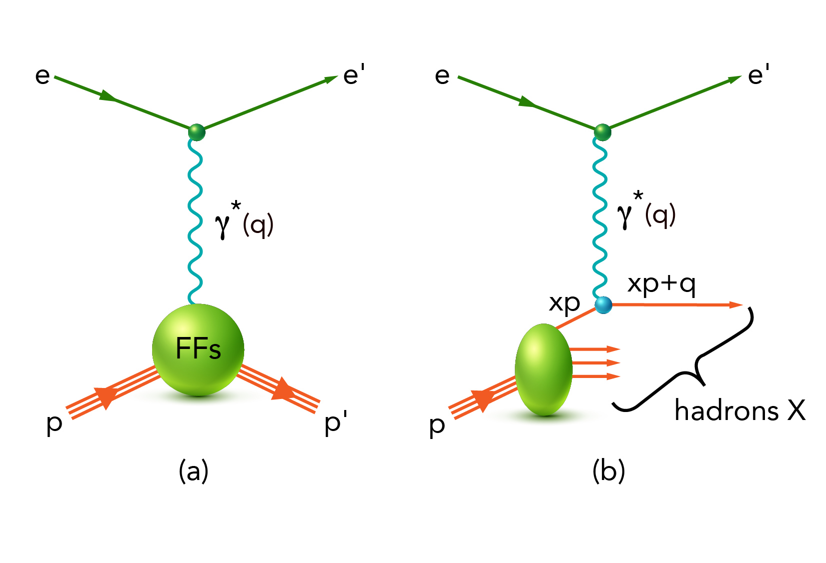
Figure 1: (a) The elastic electron-proton scattering process in which the electromagnetic form factors (FFs) are measured. (b) Inclusive deep inelastic scattering (DIS) where the proton is dissociated into a final state consisting of unresolved hadrons. In the Bjorken limit $p\cdot q\to\infty$ and $Q^{2}=-q^{2}\to\infty$ with $x_{B}=Q^{2}/(2p\cdot q)$ fixed, DIS is interpreted in the so-called infinite-momentum frame as the scattering of electrons off pointlike quarks carrying the fraction $x$ of the nucleon’s momentum, where $x=x_{B}$ up to corrections suppressed by $M_{N}^{2}/Q^{2}$.

I.2 The proton’s finite size

An important milestone in the field of nucleon structure was brought by studies of elastic electron-proton scattering, shown in Fig. 1a, which revealed early insights into the proton’s size. The deviations in scattering data from expectations for pointlike particles are encoded in terms of form factors (FFs) defined through matrix elements of the electromagnetic current operator, $\langle p^{\prime},\vec{s}^{\,\prime}|J^{\mu}_{em}|p,\vec{s}\rangle$, where $|p,\vec{s}\rangle$ is the initial state of the proton with momentum $p$ polarized along the $\vec{s}$ direction, and analogously for the final proton state.

These FFs would be constants for pointlike particles, but they were found to be pronounced functions of the Mandelstam variable $t=(p^{\prime}-p)^{2}$. A spin-$\frac{1}{2}$ particle has two electromagnetic FFs, $F_{1}(t)$ and $F_{2}(t)$, defined such that $F_{1}(0)$ is the electric charge in units of $e$, and $F_{2}(0)$ is the anomalous magnetic moment, i.e., the deviation from the value predicted by the Dirac equation, in units of $\mu_{N}$. Knowledge of the $t$-dependence of electromagnetic FFs allowed information about the spatial distributions of electric charge and magnetization to be inferred Sachs (1962) (more discussion of this interpretation can be found in Lorcé (2020); Chen and Lorcé (2022, 2023)). This led to the first determination of the proton charge radius of $(0.74\pm 0.24)\,$fm McAllister and Hofstadter (1956). These experiments have continued to this day, and, using a variety of experimental techniques, they resulted in a much more precise knowledge of the proton’s charge radius Workman et al. (2022).

I.3 Discovery of partons

The 1950s witnessed immense progress in accelerator and detection techniques followed by a proliferation of discoveries of strongly interacting particles and resonances, including particles like the antiproton, $\Delta$, and $\Xi$, see the early review Snow and M. M. Shapiro (1961). On the theory side, this led to the development of the quark model Gell-Mann (1964); Zweig (1964) in which hadrons are classified according to quantum numbers which are understood to arise from various combinations of “quarks”. The “quarks” in this model were group-theoretical objects, and their dynamics were unknown.

The next milestone was brought by high-energy experiments carried out at the Stanford Linear Accelerator, where the Bjorken scaling predicted on the basis of current algebra and dispersion relation techniques Bjorken (1969) was observed in inclusive deep inelastic scattering (DIS) Bloom et al. (1969). The response of the nucleon in DIS is described by structure functions which, on general grounds, are functions of the Lorentz invariants $p\cdot q$ and $Q^{2}=-q^{2}$, where $p^{\mu}$ is the nucleon four-momentum and $q^{\mu}$ the four-momentum transfer, see Fig. 1b. Bjorken scaling is the property that, in the high-energy limit $p\cdot q\to\infty$ and $Q^{2}\to\infty$ with their ratio fixed, the structure functions are, to a first approximation, functions of a single variable $x_{B}=Q^{2}/(2p\cdot q)$ which on kinematical grounds satisfies $0<x_{B}<1$.

The physical significance of this non-trivial observation was interpreted in the parton model Feynman (1969), where the DIS process proceeds as shown in Fig. 1b, namely the electrons scatter off nearly free electrically-charged pointlike particles called partons, with a cross-section that can be calculated in quantum electrodynamics (QED). The structure of the nucleon in DIS is described in terms of parton distribution functions (PDFs), depicted by the green ellipse in Fig. 1b. (More precisely, PDFs are defined after squaring the amplitude in Fig. 1 and summing over the complete set of states $X$.) In modern terminology, the PDFs in unpolarized DIS are denoted $f_{1}^{a}(x)$, with $a$ labelling the type of parton. More precisely, $f_{1}^{a}(x)\,\mathrm{d}x$ is the probability to find a parton of type $a$ in the initial state inside of a nucleon moving with nearly the speed of light (an appropriate picture in DIS where $x\approx x_{B}$) and carrying a fraction of the nucleon’s momentum in the interval $[x,\;x+\mathrm{d}x]$. It was soon realized that the electrically charged partons, identified with quarks and antiquarks, carry only half of the nucleon’s momentum between them.

I.4 Colored quarks and gluons, QCD, and confinement

The discovery of proton substructure and the development of the parton model were key to establishing quantum chromodynamics (QCD) as the theory of the fundamental interaction between quarks carrying $N_{c}=3$ different color charges (and antiquarks carrying the corresponding anticharges) Gross and Wilczek (1973); Politzer (1973); Fritzsch et al. (1973). The color forces are mediated by the exchange of spin-1 gluons which also carry color charges (as opposed to electrically neutral photons which mediate interactions in QED). Evidence for the existence of gluons has been found in the study of $e^{+}e^{-}$ annihilation processes Brandelik et al. (1980). Being electrically neutral, the gluons are “invisible” in interactions with electrons, and account for the missing half of the proton momentum in DIS.

The QCD Lagrangian is given by

$${\cal L}=\sum_{q}\overline{\psi}_{q}(i\not{D}+m_{q})\psi_{q}-\tfrac{1}{4}\,F^{2},$$ (1)

where $\overline{\psi}_{q}$ and $\psi_{q}$ denote the quark and antiquark fields and $m_{q}$ denotes the current quark masses. The summation runs over the quark flavors $q\in\{u,\,d,\,s,\,c,\,b,\,t\}$. The covariant derivative is defined as $iD_{\mu}=i\partial_{\mu}+gA_{\mu}^{c}T^{c}$ and $F^{2}=F^{c}_{\mu\nu}F^{c\mu\nu}$ with $F^{c}_{\mu\nu}=\partial_{\mu}A^{c}_{\nu}-\partial_{\nu}A^{c}_{\mu}+gf^{cde}A^{d}_{\mu}A^{e}_{\nu}$. Here $A_{\mu}^{c}$ are the gauge (gluon) fields and $T^{c}$ the generators in the fundamental representation of SU($N_{c}$) with $c\in\{1,\,\dots,\,N_{c}^{2}-1\}$ and $f^{cde}$ are the structure constants of the SU($N_{c}$) group. Non-abelian gauge theories like QCD are renormalizable ’t Hooft and Veltman (1972) with the coupling constant $\alpha_{s}(\mu)=g(\mu)^{2}/(4\pi)$ depending on the renormalization scale $\mu$. When it comes to describing hadrons, the scale is $\mu\sim 1\,\rm{GeV}$ and $\alpha_{s}(\mu)$ is of order unity. The interaction is thus strong and the solution of (1) requires nonperturbative techniques. However, in high-energy processes such as DIS, where the renormalization scale is identified with the hard scale of the process, $\alpha_{s}(Q)$ decreases with increasing $Q$ reaching $\alpha_{s}(91\rm{~{}GeV})\approx 0.12$ at the scale of the $Z$-boson mass. This property, known as asymptotic freedom, explains why quarks, antiquarks and gluons appear in such reactions as nearly free partons to a first approximation. The fact that free color charges are never observed in nature gave rise to the confinement hypothesis, whose theoretical explanation is still an outstanding open question.

I.5 Proton mass, spin and $D$-term

While the fundamental degrees of freedom and their interaction described in terms of the Lagrangian (1) are well-established, many questions remain open. For instance, the proton and neutron quantum numbers arise from combining 3 light quarks, $uud$ and $udd$, whose masses in the QCD Lagrangian (1) are explained by the Brout-Englert-Higgs mechanism Englert (2014); Higgs (2014). The smallness of $m_{u}\sim 2\,{\rm MeV}/c^{2}$ and $m_{d}\sim 5\,{\rm MeV}/c^{2}$, however, gives rise to one of the central questions of QCD, namely how does the nucleon mass of 940 MeV$/c^{2}$ come about? (A wide-spread misconception is that $m_{u}+m_{u}+m_{d}\sim 9\,{\rm MeV}/c^{2}$ only explains about $1\,\%$ of the proton mass. This is incorrect, as in QCD the quark mass contribution is due to the operator $m_{q}\,\overline{\psi}_{q}\psi_{q}$ which includes virtual quark-antiquark pair contributions, leading to a much larger fraction (about 10-15 %) of the proton mass as will be discussed in Sec. II.4.)

Another central question concerns the proton spin. In a “static” quark model one would naively attribute the spin $\frac{1}{2}$ of the nucleon to the spins of the quarks. In nature, due to the relatively light $u$- and $d$-quarks being confined within distances of ${\cal O}(1\,{\rm fm})$, Heisenberg’s uncertainty principle implies an ultra-relativistic motion of the quarks. It must be expected that, e.g., the orbital motion of quarks has an important role in the spin budget of the nucleon. At the quantitative level, the nucleon spin decomposition is, however, still not known precisely Ji et al. (2021).

The answers to these questions lie in the matrix elements of the energy-momentum tensor (EMT), an operator in quantum field theory of central importance that is associated with the invariance of the theory under spacetime translations. These matrix elements encode key information including the mass and spin of a particle, the less well-known but equally fundamental $D$-term ($D$ stands for the German word Druck meaning pressure), as well as information about the distributions of energy, angular momentum, and various mechanical properties such as, e.g., internal forces inside the system. These properties are encoded in the gravitational form factors. In the standard model (plus gravity) the EMT couples to gravitons, so the direct way to measure its matrix elements would be graviton-proton scattering. Since the gravitational interaction between a proton and an electron is (at currently achievable lab energies) $10^{-39}$ times weaker than their electromagnetic interaction, direct use of gravity to probe proton structure is impossible in electron-proton scattering, and in fact in any accelerator experiment in the foreseeable future. However, we have learned how to apply indirect methods to acquire information about the EMT through studies of hard exclusive reactions. The purpose of this Colloquium is to review the progress in theory, experiment, and interpretation of the EMT matrix elements. While the main focus is on the proton, also other hadrons will be discussed to provide a wider context and improve understanding.

II The energy-momentum tensor

In this section, after reviewing the definition and properties of the EMT in QCD, the gravitational form factors (GFFs) of the proton are introduced. It is shown how GFFs can be leveraged to elucidate the proton’s mass and spin decompositions.

II.1 Definition of the EMT operator

In QCD, the EMT $T^{\mu\nu}=\sum_{q}T^{\mu\nu}_{q}+T^{\mu\nu}_{G}$ can be decomposed into gauge-invariant quark and gluon parts as

$$T^{\mu\nu}_{q} =\overline{\psi}_{q}\gamma^{\mu}\,iD^{\nu}\psi_{q},$$ (2)

$$T^{\mu\nu}_{G} =-F^{c\mu\lambda}F^{c\nu}_{\phantom{c\nu}\lambda}+\tfrac{1}{4}\,g^{\mu\nu}F^{2}$$

with $g_{\mu\nu}=\text{diag}(+1,-1,-1,-1)$ the Minkowski metric. In quantum field theory, the expressions for the matrix elements of bare operators contain divergences and must be renormalized ’t Hooft and Veltman (1972). Therefore, each term in (2) is understood as a renormalized operator defined at some renormalization scale $\mu$. The components of the EMT are interpreted in the same way as in the classical theory, namely $T^{00}$ is the energy density, $T^{0i}$ is the momentum density, $T^{i0}$ is the energy flux, and $T^{ij}$ is the momentum flux or stress tensor.

Since the antisymmetric part $T^{[\mu\nu]}=\frac{1}{2}(T^{\mu\nu}-T^{\nu\mu})$ of (2) can be written as a total divergence using the equations of motion, it does not contribute to the total four-momentum and angular momentum of the system. In the literature, one often considers only the symmetric part $T^{\{\mu\nu\}}=\frac{1}{2}(T^{\mu\nu}+T^{\nu\mu})$, known as the Belinfante EMT Belinfante (1962), where the distinction between orbital angular momentum and spin is lost Leader and Lorcé (2014); Lorcé et al. (2018).

II.2 Trace anomaly

The invariance of the classical Lagrangian of a theory under a certain symmetry implies the existence of a conserved, so-called Noether, current Noether (1918). For instance, the EMT is the Noether current associated with the invariance of a theory under space-time translations. If the classical symmetry is obeyed in quantum field theory (as is the case for space-time translations) one obtains a conservation law.

If a classical symmetry is spoiled by quantum effects, then one speaks of a “quantum anomaly” and there is no associated conservation law. One important example is the trace anomaly (for another example see Sec. IV.1): the QCD Lagrangian (1) is “approximately” invariant under scale transformations $x\mapsto x^{\prime}=\lambda x$ with arbitrary $\lambda>0$. It is not an exact symmetry since the divergence of the corresponding Noether current does not vanish but is equal at the classical level to $g_{\mu\nu}T^{\mu\nu}_{\text{class}}=\sum_{q}m_{q}\,\overline{\psi}_{q}\psi_{q}$. In the light quark sector, due to the smallness of the up- and down-quark masses, one would nevertheless expect this to be a good approximate symmetry similarly to the isospin symmetry encountered in Sec. I.1. However, quantum corrections alter the trace of the EMT as Collins et al. (1977); Nielsen (1977)

$$g_{\mu\nu}T^{\mu\nu}=\sum_{q}(1+\gamma_{m})m_{q}\,\overline{\psi}_{q}\psi_{q}+\tfrac{\beta(g)}{2g}\,F^{2},$$ (3)

where $\gamma_{m}$ is the anomalous quark mass dimension and $\beta(g)=\partial g/\partial\ln\mu$ is the QCD beta function which describes how the coupling changes with the renormalization scale. As will be discussed later, the trace anomaly plays an important role for the mass and mechanical properties of the proton. For more details, see Braun et al. (2003) and Hatta et al. (2018); Tanaka (2019); Ahmed et al. (2023).

II.3 Definition of the proton gravitational form factors

The electromagnetic structure of the proton is encoded in the matrix elements of the electromagnetic current $\langle p^{\prime},\vec{s}^{\,\prime}|J^{\mu}_{em}|p,\vec{s}\rangle$. Similarly, the matrix elements of the EMT operator $\langle p^{\prime},\vec{s}^{\,\prime}|T_{a}^{\mu\nu}|p,\vec{s}\rangle$ for quarks ($a=q$) and gluons ($a=G$) allow one to study the mass and spin decompositions, as well as the mechanical properties.

Thanks to Poincaré symmetry, these matrix elements can be written as Kobzarev and Okun (1962); Pagels (1966); Ji (1997b); Bakker et al. (2004); Lorcé et al. (2022b)

$$\langle p^{\prime},\vec{s}^{\,\prime}|T_{a}^{\mu\nu}|p,\vec{s}\rangle=\overline{u}(p^{\prime},\vec{s}^{\,\prime})\Bigg{[}A_{a}(t)\,\frac{P^{\mu}P^{\nu}}{M_{N}}$$ (4)

$$+D_{a}(t)\,\frac{\Delta^{\mu}\Delta^{\nu}-g^{\mu\nu}\Delta^{2}}{4M_{N}}+\bar{C}_{a}(t)\,M_{N}\,g^{\mu\nu}$$

$$+J_{a}(t)\ \frac{P^{\{\mu}i\sigma^{\nu\}\lambda}\Delta_{\lambda}}{M_{N}}-S_{a}(t)\ \frac{P^{[\mu}i\sigma^{\nu]\lambda}\Delta_{\lambda}}{M_{N}}\Bigg{]}u(p,\vec{s})$$

with $P=(p^{\prime}+p)/2$ and $\Delta=p^{\prime}-p$ the symmetric kinematical variables, $u(p,\vec{s})$ the usual free Dirac spinor, and $M_{N}$ the nucleon mass. The Lorentz-invariant functions $A_{a}(t)$, $D_{a}(t)$, $\bar{C}_{a}(t)$, $J_{a}(t)$ and $S_{a}(t)$ depend on the square of the four-momentum transfer $t=\Delta^{2}$. They are the EMT analogues of the more familiar electromagnetic FFs, and are accordingly called gravitational form factors (GFFs). In contrast to the electromagnetic FFs, these GFFs inherit also a renormalization scale dependence from the associated operators, which is omitted in the notation for convenience. The total GFFs $\sum_{a}A_{a}(t)$, $\sum_{a}D_{a}(t)$, $\sum_{a}\bar{C}_{a}(t)$ and $\sum_{a}J_{a}(t)$ are, however, renormalization scale independent Nielsen (1977).

On top of restricting the number of GFFs, Poincaré symmetry imposes additional constraints, namely

$$A(0) = \sum_{q}A_{q}(0)+A_{G}(0)=1,$$ (5)

$$J(0) = \sum_{q}J_{q}(0)+J_{G}(0)=\tfrac{1}{2},$$ (6)

$$\tfrac{1}{2}\Delta\Sigma = \sum_{q}S_{q}(0),$$ (7)

$$\bar{C}(t) = \sum_{q}\bar{C}_{q}(t)+\bar{C}_{G}(t)=0,$$ (8)

where (5) follows from translation symmetry Ji (1998), while (6) and (7) result from Lorentz symmetry Ji (1997b); Bakker et al. (2004), with $\tfrac{1}{2}\Delta\Sigma$ denoting the quark spin contribution to the nucleon spin. The constraint (8), valid for any $t$, follows from EMT conservation $\partial_{\mu}T^{\mu\nu}=0$. Interestingly, the renormalization-scale invariant quantity Polyakov and Weiss (1999)

$$D\equiv D(0)=\sum_{q}D_{q}(0)+D_{G}(0),$$ (9)

known as the $D$-term, is a global property of the proton (and, in fact, any hadron), whose value is not fixed by spacetime symmetries Polyakov and Weiss (1999). Its physical interpretation will be discussed in Sec. VI.

Until recently, the only information about GFFs known from phenomenology was $A_{a}(0)=\int_{-1}^{1}\mathrm{d}x\,x\,f^{a}_{1}(x)$, corresponding to the fraction of proton momentum carried by the partons $a$ as inferred from DIS experiments, and $S_{q}(0)=\frac{1}{2}\int_{-1}^{1}\mathrm{d}x\,g^{q}_{1}(x)$, where $g^{q}_{1}(x)$ is the quark helicity distribution Aidala et al. (2013).

II.4 Decomposition of proton mass

Just like the charge density is defined via a Fourier transform of the matrix elements of the electromagnetic current, the spatial distributions of energy and momentum read Polyakov (2003); Polyakov and Schweitzer (2018b); Lorcé et al. (2019)

$$\mathcal{T}^{\mu\nu}_{a}(\vec{r})=\int\frac{\mathrm{d}^{3}\Delta}{(2\pi)^{3}2E}\,e^{-i\vec{\Delta}\cdot\vec{r}}\,\langle p^{\prime}|T^{\mu\nu}_{a}|p\rangle$$ (10)

in the so-called Breit frame defined by the conditions $\vec{p}^{\,\prime}=-\vec{p}=\vec{\Delta}/2$ and $p^{\prime 0}=p^{0}=E=\sqrt{M_{N}^{2}+\vec{\Delta}^{2}/4}$. For ease of notation, the dependence on the nucleon polarization is omitted. Integrating over space, one obtains

$$\int\mathrm{d}^{3}r\,\mathcal{T}^{\mu\nu}_{a}(\vec{r})=\frac{\langle p|T^{\mu\nu}_{a}|p\rangle}{2M_{N}}\bigg{|}_{\vec{p}=\vec{0}}$$ (11)

i.e., the matrix elements for the proton at rest. More explicitly, one finds

$$\int\mathrm{d}^{3}r\,\mathcal{T}^{\mu\nu}_{a}(\vec{r})=\begin{pmatrix}U_{a}&0&0&0\\ 0&W_{a}&0&0\\ 0&0&W_{a}&0\\ 0&0&0&W_{a}\end{pmatrix}.$$ (12)

The components $\mathcal{T}^{00}(\vec{r})$ and $\frac{1}{3}\sum_{i}\mathcal{T}^{ii}(\vec{r})$ represent the energy density and the isotropic pressure in the system, and so $U_{a}=\int\mathrm{d}^{3}r\,\mathcal{T}^{00}_{a}(\vec{r})=[A_{a}(0)+\bar{C}_{a}(0)]\,M_{N}$ and $W_{a}=\frac{1}{3}\sum_{i}\int\mathrm{d}^{3}r\,\mathcal{T}^{ii}_{a}(\vec{r})=-\bar{C}_{a}(0)M_{N}$ are respectively interpreted as the quark or gluon contributions to internal energy and pressure-volume work.

Since by definition $p^{2}=M_{N}^{2}$, the proton mass can be identified with the total energy in the rest frame

$$\sum_{a}U_{a}=M_{N}.$$ (13)

Moreover, the proton being a bound state at mechanical equilibrium, the virial theorem says that the total pressure-volume work must vanish Laue (1911); Lorcé (2018a); Lorcé et al. (2021)

$$\sum_{a}W_{a}=0.$$ (14)

These are two independent sum rules underlying the various mass decompositions proposed in the literature, see Lorcé et al. (2021) for a detailed review. To keep the following discussion as simple as possible, the standard $\overline{\text{MS}}$ scheme with the additional requirement that the trace anomaly arises purely from the gluonic sector is used in the following Metz et al. (2020); Lorcé et al. (2021).

Defining the quark mass contribution to the nucleon mass via

$$M_{m}=\sum_{q}\sigma_{q}\equiv\frac{\langle p|\sum_{q}m_{q}\,\overline{\psi}_{q}\psi_{q}|p\rangle}{2M_{N}}\bigg{|}_{\vec{p}=\vec{0}},$$ (15)

one obtains a three-term mass decomposition directly from the energy sum rule (13)

$$M_{N}=\sum_{q}M_{q}+M_{m}+M_{G},$$ (16)

where $M_{q}=U_{q}-\sigma_{q}$ and $M_{G}=U_{G}$ can, respectively, be interpreted as the kinetic+potential energies of quarks and gluons Rodini et al. (2020); Metz et al. (2020). Motivated by the fact that the traceless part of the gluon EMT can directly be accessed in high-energy experiments, a further of decomposition of the gluon energy

$$M_{G}=\bar{M}_{G}+\tfrac{1}{4}M_{A}$$ (17)

into the traceless part $\bar{M}_{G}=\frac{3}{4}(U_{G}+W_{G})=\tfrac{3}{4}A_{G}(0)M_{N}$ and pure trace part $\frac{1}{4}M_{A}=\frac{1}{4}(U_{G}-3W_{G})$ has been proposed in Ji (1995a, b, 2021). Since at the classical level the gluon EMT is traceless, $\bar{M}_{G}$ was interpreted as the “classical” gluon energy and $\frac{1}{4}M_{A}$ with

$$M_{A}=\frac{\langle p|\sum_{q}\gamma_{m}m_{q}\,\overline{\psi}_{q}\psi_{q}+\frac{\beta(g)}{2g}\,F^{2}|p\rangle}{2M_{N}}\bigg{|}_{\vec{p}=\vec{0}}$$ (18)

as the “quantum anomalous energy”. This interpretation is, however, not supported by a careful analysis in the $\overline{\text{MS}}$ scheme. Indeed, at the level of renormalized operators, it is the total gluon energy density (and not its traceless part) that has the familiar form $T^{00}_{G}=\frac{1}{2}(\vec{E}^{2}+\vec{B}^{2})$, ensuring that time translation symmetry remains exact under renormalization Nielsen (1977); Suzuki (2013); Tanaka (2019); Metz et al. (2020); Lorcé et al. (2021); Ahmed et al. (2023); Tanaka (2023). A recent explicit one-loop calculation within the scalar diquark model Amor-Quiroz et al. (2023) confirms that, unlike the EMT trace, the total energy does not receive any intrinsic anomalous contribution.

Since mass is a Lorentz-invariant quantity, one sometimes prefers to start from the trace of the EMT

$$\langle p|g_{\mu\nu}T^{\mu\nu}|p\rangle=2p^{2}=2M_{N}^{2}$$ (19)

and then decompose it into quark and gluon contributions Shifman et al. (1978); Donoghue et al. (2014); Hatta et al. (2018); Tanaka (2019), leading to the sum rule

$$M_{N}=M_{m}+M_{A}.$$ (20)

Current phenomenology Hoferichter et al. (2016) and Lattice QCD calculations Alexandrou et al. (2020b) indicate that $M_{m}/M_{N}\approx 10\%$, suggesting that most of the proton mass comes from the trace anomaly (and hence from the gluons, since $\gamma_{m}$ is small). To clarify the actual meaning of this result, it has been noted in Lorcé (2018a) that the sum rule (20) is equivalent to writing

$$M_{N}=\sum_{a}\int\mathrm{d}^{3}r\,g_{\mu\nu}\mathcal{T}^{\mu\nu}_{a}(\vec{r})=\sum_{a}\left(U_{a}-3W_{a}\right).$$ (21)

While the total pressure-volume work vanishes owing to the virial theorem (14), it does nevertheless contribute to the separate quark and gluon contributions to the EMT trace. Since $\sum_{q}U_{q}$ and $U_{G}$ turn out to be of the same order of magnitude, the smallness of $M_{m}$ relative to $M_{A}$ indicates in reality that $\sum_{q}W_{q}=-W_{G}>0$. In other words, the net quark force is repulsive and is exactly balanced by the net attractive gluon force.

Since the four-momentum (and hence the mass) of a system is defined via the $T^{0\mu}$ components of the EMT, it has been argued in Lorcé (2018a); Lorcé et al. (2021) that a genuine mass decomposition should in principle not entail the components $T^{ii}$. In particular, the quantities $\bar{M}_{g}$ and $M_{A}$ involve the gluon pressure-volume work $W_{g}$, and hence do not have a clean interpretation as mass contributions. From this point of view, both (17) and (20) should rather be regarded as mere sum rules mixing the genuine mass decomposition (16) with the virial theorem (14).

II.5 Decomposition of proton spin

A similar discussion elucidates the proton spin decomposition. The total angular momentum (AM) operator is defined, in terms of the Belinfante (symmetric) EMT $T^{\mu\nu}_{\text{Bel}}=T^{\{\mu\nu\}}$, as

$$\mathcal{J}^{i}=\int\mathrm{d}^{3}r\,\epsilon^{ijk}r^{j}T^{0k}_{\text{Bel}}.$$ (22)

Because of the explicit factor of $r^{j}$, the expectation value of this operator in a momentum eigenstate turns out to be ill-defined. A proper treatment requires the use of wave packets and amounts to considering matrix elements with non-vanishing momentum transfer Bakker et al. (2004); Leader and Lorcé (2014).

For convenience, only the longitudinal AM (i.e., the component along the proton average momentum $\vec{P}=\frac{1}{2}(\vec{p}^{\,\prime}+\vec{p})$ defining the $z$-direction) is considered here. The discussion about the transverse AM turns out to be much more complex because of its dependence on both $|\vec{P}|$ and the choice of origin, see e.g. Lorcé (2018b, 2021) and references therein. From the splitting of the EMT in (2), one finds that the quark and gluon contributions to the proton spin $\langle\mathcal{J}^{z}\rangle=\sum_{q}J^{z}_{q}+J^{z}_{G}$ are given by Ji (1997b)

$$J^{z}_{a}=J_{a}(0),$$ (23)

for a proton polarized in the $z$-direction.

Working instead with an asymmetric EMT, the quark AM operator can be further decomposed into orbital and intrinsic AM terms

$$\mathcal{J}^{i}_{q}=\int\mathrm{d}^{3}r\,\epsilon^{ijk}r^{j}T^{0k}_{q}+\int\mathrm{d}^{3}r\,\tfrac{1}{2}\overline{\psi}_{q}\gamma^{i}\gamma_{5}\psi_{q}.$$ (24)

Calculating the corresponding matrix elements, one then finds that $J^{z}_{q}=L^{z}_{q}+S^{z}_{q}$ with

$$L^{z}_{q} =J_{q}(0)-S_{q}(0),$$ (25)

$$\sum_{q}S^{z}_{q} =\tfrac{1}{2}\Delta\Sigma.$$

Combining the results (24) and (25) with the fact that the proton is a spin-$\frac{1}{2}$ particle, one arrives at the constraints given in (6) and (7).

Since gluons are spin-$1$ particles, one may wonder whether the gluon AM could also be decomposed into orbital and intrinsic contributions. This can be done, but it requires non-local operators to preserve gauge invariance Chen et al. (2008); Hatta (2012); Lorcé (2013a, b); Leader and Lorcé (2014); Wakamatsu (2014). One is then led to the canonical (or Jaffe-Manohar) spin decomposition Jaffe and Manohar (1990), to be distinguished from the one derived here from the local EMT (2) and known as the kinetic (or Ji) spin decomposition Ji (1997b). Finally, it is possible to push this analysis further and study the spatial distribution of angular momentum Lorcé et al. (2018).

III Measuring gravitational form factors

There is no direct way to measure the proton GFFs, as it would require measurements of the graviton-proton interaction Kobzarev and Okun (1962); Pagels (1966). More recent theoretical developments have shown, however, that the GFFs may be probed indirectly in various exclusive processes. This is the subject of this section.

III.1 Deeply virtual Compton scattering (DVCS)

In DVCS, the most explored process so far that accesses the GFFs, high-energy charged leptons scatter off protons or nuclei by exchanging a deeply virtual photon, producing a real photon in the final state Müller et al. (1994); Radyushkin (1996); Ji (1997a). Similarly to DIS (see I.C), in the high-energy limit defined by $Q^{2}\to\infty$ and $P\cdot q\to\infty$ with $(-t)\ll Q^{2}$ and $P=(p^{\prime}+p)/2$, the process is described in QCD Collins and Freund (1999) in terms of the upper part of the handbag diagram shown in Fig. 2a, which can be calculated in perturbative QCD, and a lower part described in terms of generalized parton distributions (GPDs). GPDs are universal, i.e., the same non-perturbative functions enter the description of different hard exclusive reactions.

GPDs are functions of $x$, $\xi$, and $t$. The new quantity $\xi\approx x_{B}/(2-x_{B})$ in the high energy limit, called skewness, represents the longitudinal momentum transfer to the struck quark from the initial to final state (see Fig. 2a). The variables $\xi$ and $t$ are observable in DVCS, while $x$ is not observable and enters the DVCS amplitude as an integration variable. GPDs encompass both PDFs and electromagnetic FFs discussed in Sec. I. For $p^{\prime}\to p$ implying $\xi\to 0$ and $t\to 0$, GPDs reduce to PDFs; integrating the GPDs over $x$ yields the electromagnetic FFs.

GPDs parameterize the matrix elements of certain non-local operators which can be expanded in terms of a series of local operators with various $J^{PC}$ quantum numbers. This includes operators with the quantum numbers of the graviton ($J=2$), and so part of the information about how the proton would interact with a graviton is encoded within this tower. As the electromagnetic coupling to quarks is many orders of magnitude stronger than gravity, the DVCS process is an effective tool to probe the proton’s gravitational properties. Gluon GPDs are accessible in DVCS only at higher orders in $\alpha_{s}$.

The leading contribution to DVCS is described in terms of four GPDs. Two of them, namely $H_{q}(x,\xi,t)$ and $E_{q}(x,\xi,t)$, give access to the quark GFFs as follows

$$\int_{-1}^{1}\mathrm{d}x\,xH_{q}(x,\xi,t)=A_{q}(t)+\xi^{2}D_{q}(t),$$ (26)

$$\int_{-1}^{1}\mathrm{d}x\,xE_{q}(x,\xi,t)=B_{q}(t)-\xi^{2}D_{q}(t),$$

where $B_{q}(t)=2J_{q}(t)-A_{q}(t)$ is the quark contribution to the proton’s anomalous gravitomagnetic moment. Analogous relations hold for gluons, and $B(0)=\sum_{a}B_{a}(0)$ vanishes due to Eqs. (5) and (6) Kobzarev and Okun (1962); Teryaev (1999); Brodsky et al. (2001); Lowdon et al. (2017); Cotogno et al. (2019); Lorcé and Lowdon (2020).

The actual observables in DVCS are Compton form factors (CFFs) which are expressed by means of factorization formulae in terms of complex-valued convolution integrals given, at leading order $\alpha_{s}$, by

$$\text{Re}{\mathcal{H}}(\xi,t)+i\,\text{Im}{\mathcal{H}}(\xi,t)=\\ \sum_{q}e^{2}_{q}\int_{-1}^{1}dx\left[\frac{1}{\xi-x-i\epsilon}-\frac{1}{\xi+x-i\epsilon}\right]H_{q}(x,\xi,t),$$ (27)

and similarly for the other GPDs. The CFFs are related to measurable quantities such as differential cross sections and beam and target polarization asymmetries.

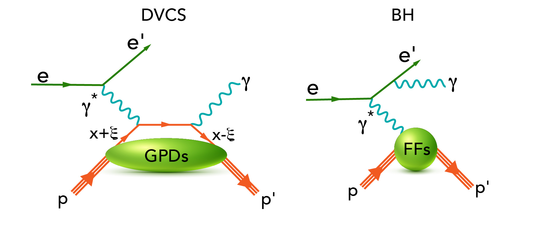
(a)                                  (b)

Figure 2: (a) QCD factorization of the DVCS amplitude. The perturbatively calculable “hard part” is shown to lowest order in the strong coupling. The nonperturbative “soft part” is described by the universal quark GPDs. (b) One of the QED diagrams for the amplitude of the Bethe-Heitler process, which has the same final state as DVCS and interferes with it. The Bethe-Heitler process is calculable requiring only the proton electromagnetic FFs as input.

The DVCS cross section is typically very small. Fortunately, DVCS interferes with the Bethe-Heitler process, see Fig. 2b, which can be computed in QED given the proton’s electromagnetic FFs, and has the same final state but with the final state photon emitted from the electron lines. The interference term projects out Im${\mathcal{H}(\xi,t)}$ when a spin-polarized electron beam is employed, while Re${\mathcal{H}(\xi,t)}$ contributes dominantly to the unpolarized DVCS cross section, and may be constrained through precise unpolarized cross section measurements.

The convolution integrals like (27) cannot be inverted in a model-independent way to yield GPDs Bertone et al. (2021). However, with experimental information from other exclusive processes becoming available (to be discussed below), the GPDs may be further constrained. Presently, a model-independent extraction of the GPDs and, via (26), of the GFFs $A_{q}(t)$ and $J_{q}(t)$ is not possible. In the case of the GFF $D_{q}(t)$, however, the situation is more fortunate. In particular, the real and imaginary parts of ${\mathcal{H}(\xi,t)}$ are related by the fixed-$t$ dispersion relation Diehl and Ivanov (2007); Anikin and Teryaev (2008)

$${\rm Re}{\mathcal{H}}(\xi,t)=\mathcal{C}_{\mathcal{H}}(t)\\ +\frac{1}{\pi}\,{\text{P.V.}}\int_{0}^{1}\text{d}\xi^{\prime}\left[\frac{1}{\xi-\xi^{\prime}}-\frac{1}{\xi+\xi^{\prime}}\right]{\rm Im}{\mathcal{H}}(\xi^{\prime},t),$$ (28)

where P.V. denotes the Cauchy’s principal value of the integral. This expression contains a real subtraction term $\mathcal{C}_{\mathcal{H}}(t)$ given by

$$\mathcal{C}_{\mathcal{H}}(t)=2\sum_{q}e^{2}_{q}\int_{-1}^{1}\mathrm{d}z\,\frac{D^{q}_{\text{term}}(z,t)}{1-z},$$ (29)

where $D^{q}_{\text{term}}(z,t)$, originally introduced in Polyakov and Weiss (1999) and further elucidated in Teryaev (2001), has the expansion Goeke et al. (2001)

$$D^{q}_{\text{term}}(z,t)=(1-z^{2})\sum_{\text{odd}\,n}d^{q}_{n}(t)\,C^{3/2}_{n}(z)$$ (30)

with $C^{\alpha}_{n}(z)$ the Gegenbauer polynomials which diagonalize the leading-order evolution equations (the renormalization scale dependence is not indicated throughout this work). In the limit of renormalization scale $\mu\to\infty$, all $d^{q}_{n}(t)$ go to zero except $d^{q}_{1}(t)$, which is related to the GFF $D_{q}(t)$ as follows

$$D_{q}(t)=\frac{4}{5}\,d^{q}_{1}(t)=\int_{-1}^{1}\mathrm{d}z\,z\,D^{q}_{\text{term}}(z,t)\,.$$ (31)

Thus, extracting information on Im${\mathcal{H}(\xi,t)}$ and Re${\mathcal{H}(\xi,t)}$ and their scale dependence from experimental data provides access to the GFF $D_{q}(t)$.

III.2 DVCS with positron and electron beams

When data with both positron and electron beams are available, it is possible to measure the beam charge asymmetry $A_{C}$ defined as the difference in the $ep\to ep\gamma$ cross section when measured with an electron beam and measured with a positron beam, divided by their sum

$$A_{C}=\frac{\sigma^{e^{-}}-\sigma^{e^{+}}}{\sigma^{e^{-}}+\sigma^{e^{+}}}.$$ (32)

The numerator of $A_{C}$ is given by the real part of the DVCS and Bethe-Heitler interference term providing the cleanest access to Re$\mathcal{H}$ Kivel et al. (2001); Belitsky et al. (2002). In contrast to this, in DVCS measured with electrons (or positrons) alone, additional theoretical assumptions in the CFF extraction procedure are unavoidable Burkert et al. (2021a).

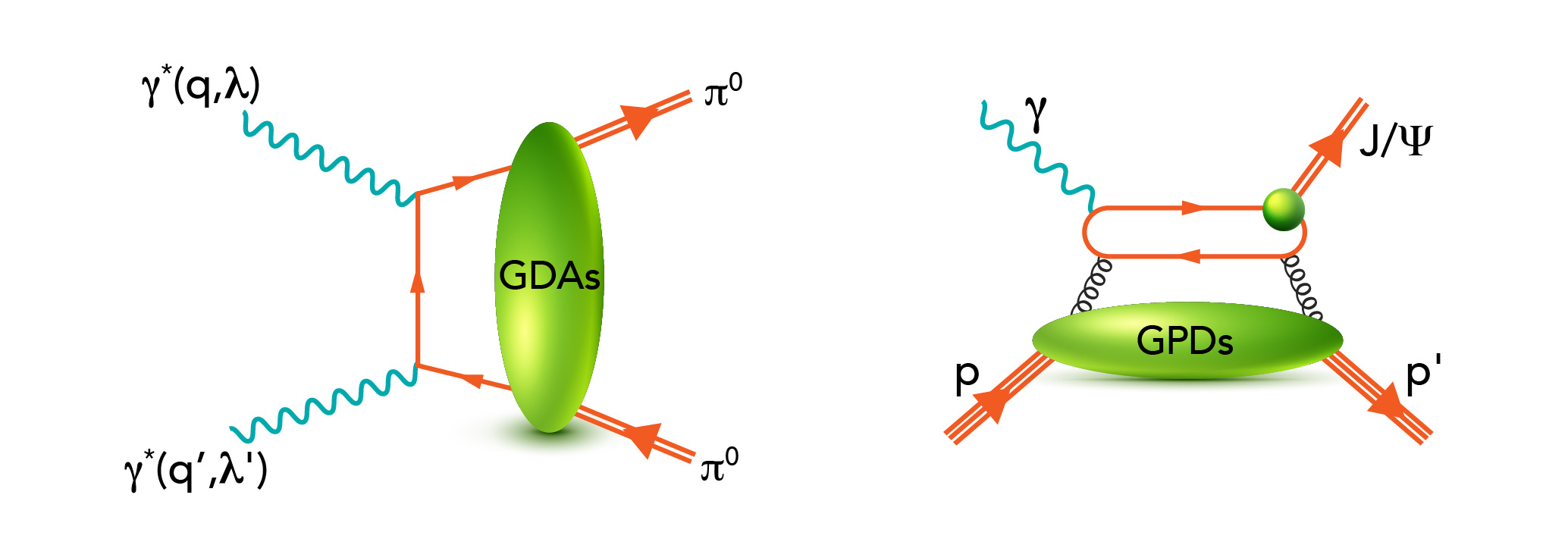
(a)                                        (b)

Figure 3: (a) The process $\gamma\gamma^{\ast}\to\pi^{0}\pi^{0}$ is described in terms of generalized distribution amplitudes, which provide access to GFFs in the time-like region $t>0$. (b) Threshold $J/\Psi$ photo-production on the proton. This process is sensitive to the gluon GPDs.

III.3 $\gamma\gamma^{\ast}\to\pi^{0}\pi^{0}$

The process $\gamma\gamma^{\ast}\to\pi^{0}\pi^{0}$ shown in Fig. 3a can be studied, e.g., at electron-positron colliders, and is described in terms of generalized distribution amplitudes which correspond to GPDs continued analytically from the $t$- to the $s$-channel Müller et al. (1994); Diehl et al. (1998). In this way, one can access information on GFFs in the time-like region where $t>0$ Kumano et al. (2018); Lorcé et al. (2022a). This process provides a unique opportunity to study the structure of unstable hadrons like pions that are not available as targets.

III.4 Time-like Compton scattering and double DVCS

Several other processes provide complementary information about the nucleon GFFs. One of them is time-like Compton scattering (TCS), $\gamma p\to p^{\prime}\gamma^{\ast}$, where the final state virtual photon produces an $e^{+}e^{-}$ pair Berger et al. (2002); Pire et al. (2011); Chatagnon et al. (2021). In TCS, Im$\mathcal{H}$ can be accessed through the polarized beam spin asymmetry and Re$\mathcal{H}$ through a forward-backward asymmetry of the final-state $e^{+}e^{-}$ pair in its centre-of-mass frame.

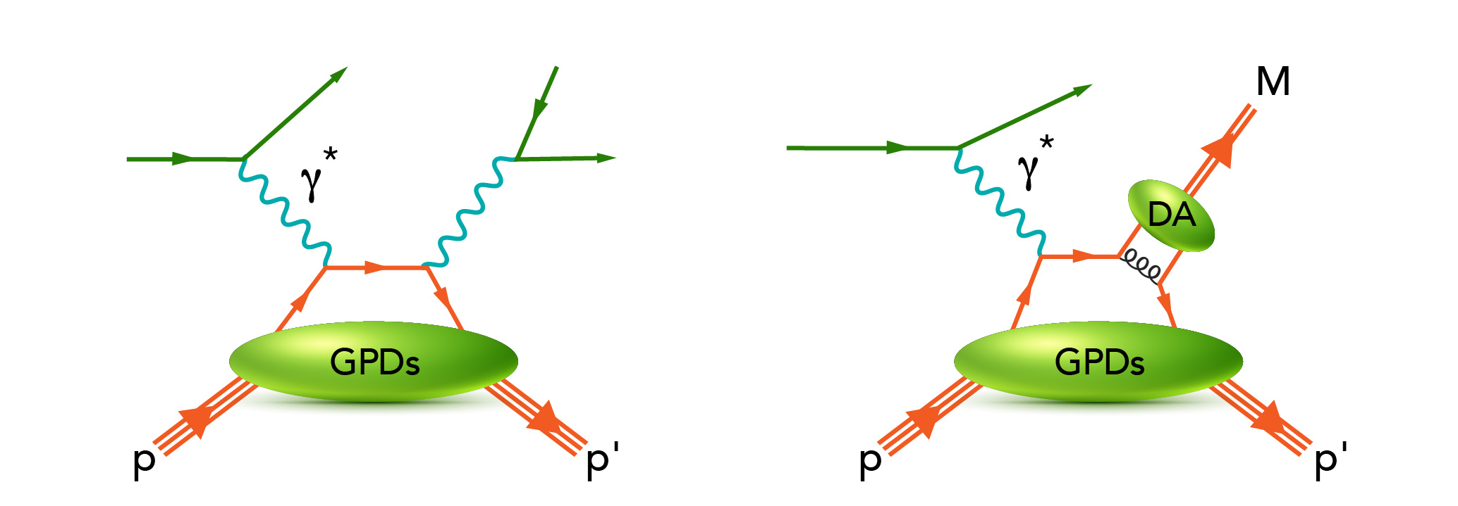
(a)                                          (b)

Figure 4: The leading double DVCS diagram (a) and one of the leading diagrams for deeply virtual meson production (b). The ellipse where the meson M is produced is the nonperturbative distribution amplitude DA.

The double DVCS process Belitsky and Müller (2003); Guidal and Vanderhaeghen (2003) displayed in Fig. 4a may also play an important role at future facilities. It is a variant of DVCS with the final-state time-like photon converting into a $e^{+}e^{-}$ or $\mu^{+}\mu^{-}$ pair. While in DVCS the GPDs are sampled along the lines $x=\pm\xi$ in the convolution integrals (27), this constraint is relaxed in double DVCS due to the variable invariant mass of the lepton pair. This is an advantage of this process, and will be of importance for less model-dependent global extractions of GPDs.

III.5 Meson production

Deeply virtual meson production Collins et al. (1997) is another process sensitive to GPDs, see Fig. 4b. Production of different vector mesons provides sensitivity to GPDs of different quark flavors which is an advantage over DVCS. However, this process is more difficult to analyze than DVCS since gluons contribute on the same footing as quarks (Fig. 4b only shows a quark diagram) and one in general expects larger power corrections. Also the process of heavy vector quarkonium photoproduction was shown to factorize in the heavy quark limit at one-loop order in perturbative QCD Ivanov et al. (2004).

Exclusive $J/\Psi$ photo-production at threshold, is expected to be sensitive to gluon GFFs Kharzeev (1996, 2021) and more generally, as depicted in Fig. 3b, to gluon GPDs Hatta and Yang (2018); Guo et al. (2021), which in DVCS are accessible only at higher orders in $\alpha_{s}$.

Gluon GFFs have recently been extracted from this process by Duran et al. (2023), but the link with the physical observables is not direct and requires approximations Sun et al. (2021, 2022), similarly to DVCS. $J/\Psi$ photoproduction can also be studied with quasi-real photons of virtualities as low as $Q^{2}\lesssim 0.1\,{\rm GeV}^{2}$ emitted by electrons, together with electroproduction and DVCS.

Finally, a new class of hard scattering processes with multi-particle final states has recently emerged Qiu and Yu (2022); Pedrak et al. (2020); Grocholski et al. (2022); Ivanov et al. (2002); Boussarie et al. (2017); Duplančić et al. (2018). Those reactions are theoretically appealing, but measuring them is challenging.

The relatively recent progress reviewed here paved the way to the exciting and even more recent experimental developments, which will be reviewed in Sec. V with a focus on DVCS and TCS. Before continuing, the next section is devoted to the theory of GFFs, whose history is equally interesting and began much earlier.

IV Theoretical Results

GFFs were introduced by Kobzarev and Okun (1962) who considered spin-0 and spin-$\frac{1}{2}$ particles and parity-violating weak effects (not discussed here), proved the vanishing of proton’s anomalous gravitomagnetic moment $B(0)=0$, and showed that one would need energies around the Planck scale to measure GFFs in gravitational interactions. This section presents an overview of GFFs from the theory perspective with particular focus on $D(t)$, the least known of the total GFFs. Despite the focus on the proton, it will be insightful to mention other hadrons for comparison when appropriate.

IV.1 Chiral symmetry and the $D$-term of the pion

GFFs received little attention from the community until it was realized that matrix elements such as $\langle\pi,\pi|T^{\mu\nu}|0\rangle$ enter the QCD description of hadronic decays of charmonia Novikov and Shifman (1981); Voloshin and Zakharov (1980) or the decay of a hypothetical light Higgs boson, an idea entertained in the early 1990s when the possibility of a light Higgs was not yet experimentally excluded Donoghue et al. (1990). These matrix elements are related to pion GFFs in the timelike region $t>0$.

In general, hadronic EMT matrix elements cannot be computed analytically in QCD, but the pion is a notable exception. The QCD Lagrangian (1) exhibits a classical symmetry under global left- and right-handed rotations in the flavor space of up, down and strange quarks. This symmetry is approximate due to the small but non-zero quark masses $m_{q}$. If this symmetry were realized in nature, then for example the nucleon state N(940) (here N stands for a state with nucleon isopin quantum number and the number in the brackets is the rounded mass of the state in ${\rm GeV}/c^{2}$) with the spin-parity quantum numbers $J^{P}={\frac{1}{2}}^{+}$ should have the same mass as its negative-parity partner $N(1535)$ with $J^{P}={\frac{1}{2}}^{-}$ modulo small corrections due to the small $m_{q}$. However, the latter is almost 600 MeV$/c^{2}$ heavier than the nucleon, an effect that cannot be attributed to current quark mass effects. The phenomenon that a symmetry of the Lagrangian is not realized in the particle spectrum is known as spontaneous symmetry breaking Nambu and Jona-Lasinio (1961a, b). It is accompanied by the emergence of massless Goldstone bosons, corresponding in QCD to pions, kaons, and $\eta$-mesons, which are not massless but are very light compared to other hadrons.

In theoretical calculations, chiral symmetry is a powerful tool allowing one to evaluate the matrix elements of Goldstone bosons in the chiral limit (and for $t\to 0$). In this way, one obtains for the pion (and kaon and $\eta$) $D$-term Novikov and Shifman (1981)

$$\lim\limits_{m_{\pi}\to 0}D_{\pi}=-1.$$ (33)

Deviations from the chiral limit are systematically calculable in chiral perturbation theory Donoghue and Leutwyler (1991) and are expected to be small for pions and more sizable for kaons and the $\eta$-meson Hudson and Schweitzer (2017). The relation between the stability of the pion and spontaneous chiral symmetry breaking was discussed by Son and Kim (2014), and the gravitational interactions of Goldstone bosons were studied by Voloshin and Dolgov (1982); Leutwyler and Shifman (1989). For hadrons other than pions, the techniques based on the chiral limit of QCD cannot predict the $D$-term, but they can still be explored to provide insights on some properties of $D(t)$, as will be discussed in Sec. IV.3.

IV.2 GFFs in model studies

Interest in GFFs was once again renewed after it was shown that they can be inferred from hard-exclusive reactions via GPDs and play a key role for the understanding of the mass and spin structure of the proton, see Sec. II, and further stimulated by their interpretation in terms of forces inside hadrons Polyakov (2003). The first model study of proton GFFs was presented by Ji et al. (1997) in the bag model, followed by works in the chiral quark-soliton model Petrov et al. (1998); Schweitzer et al. (2002); Ossmann et al. (2005); Goeke et al. (2007a, b); Wakamatsu (2007); Kim and Kim (2021) and Skyrme models Cebulla et al. (2007); Jung et al. (2014a); Perevalova et al. (2016).

Extensive GFF model studies for the nucleon and other hadrons were presented in light-front constituent quark models Pasquini and Boffi (2007); Sun and Dong (2020), diquark approaches Hwang and Müller (2008); Kumar et al. (2017); Chakrabarti et al. (2020); Choudhary et al. (2022); Fu et al. (2022); Amor-Quiroz et al. (2023), holographic AdS/QCD models Abidin and Carlson (2008, 2009); Brodsky and de Teramond (2008); Chakrabarti et al. (2015); Mondal (2016); Mondal et al. (2016); Mamo and Zahed (2020, 2021, 2022); Fujita et al. (2022), a large-$N_{c}$ bag model Neubelt et al. (2020); Lorcé et al. (2022b), a cloudy bag model Owa et al. (2022), light-cone QCD sum rules Anikin (2019); Azizi and Özdem (2020); Aliev et al. (2021); Azizi and Özdem (2021); Özdem and Azizi (2020), the Nambu–Jona-Lasinio model Freese et al. (2019), chiral quark-soliton model with strange and heavier quarks Kim et al. (2021); Won et al. (2022); Ghim et al. (2023), a dual model with complex Regge trajectories Fiore et al. (2021) and in an instant-form relativistic impulse approximation approach Krutov and Troitsky (2021, 2022). Algebraic GPD Ansätze were used to shed light on pion and kaon GFFs Raya et al. (2022) and toy models Kim et al. (2023) as well as light-cone convolution models Freese and Cosyn (2022a) were used to study the deuteron GFFs.

The $D$-terms of nuclei were studied in the liquid-drop model Polyakov (2003), revealing that for nuclei $D(0)\propto A^{7/3}$ grows strongly with mass number $A$. Studies in the Walecka model Guzey and Siddikov (2006) support this prediction which can be tested in DVCS experiments with nuclear targets. Different results were obtained in a non-relativistic nuclear spectral function approach Liuti and Taneja (2005). Nuclear GFFs were also investigated in Skyrme model frameworks Kim et al. (2012); Jung et al. (2014b); Kim et al. (2022); Garcia Martin-Caro et al. (2023).

The GFFs for a constituent quark were studied in a light-front Hamiltonian approach More et al. (2022, 2023) which, after rescaling and regularization of infrared divergences, reproduces QED results for an electron Metz et al. (2021); Freese et al. (2023). GFFs of the photon in QED were studied in Friot et al. (2007); Gabdrakhmanov and Teryaev (2012); Polyakov and Sun (2019); Freese and Cosyn (2022b). An insightful model for composite particles is the $Q$-ball system where stable, metastable, unstable states were investigated, showing that, among all studied particle properties, $D(0)$ is most sensitive to details of the dynamics Mai and Schweitzer (2012a, b); Cantara et al. (2016). Remarkably, the same conclusions were obtained in the bag model where, e.g., for the $N^{\rm th}$ highly excited nucleon state the mass increases as $M\propto N^{3}$ whereas $D(0)\propto N^{8}$ grows much more strongly with $N$ Neubelt et al. (2020).

IV.3 Limits in QCD and dispersion relations

Model-independent results for GFFs can be obtained in certain limiting situations in QCD, e.g., when the number of colors $N_{c}\to\infty$ or when $|t|$ becomes very small or very large, and through the use of dispersion relation methods. These methods are complementary to the nonperturbative lattice QCD methods which are reviewed in the next section.

In the large-$N_{c}$ limit of QCD, baryons are described as solitons of mesonic fields Witten (1979). Large-$N_{c}$ QCD has not been solved (in 3+1 dimensions) and the soliton field is not known (though it can be modelled). Nontrivial results can, however, be derived based on the known symmetries of the large-$N_{c}$ soliton field which are generally well-supported in nature Dashen et al. (1994) despite $N_{c}=3$. The relations of the GFFs of the nucleon and $\Delta$ were studied in the large-$N_{c}$ limit of QCD in Panteleeva and Polyakov (2020). The GFFs of the $\Delta$ are difficult to measure, but such relations can be tested, e.g., in soliton models like the chiral quark-soliton model or Skyrme model (mentioned in the previous subsection) or in lattice QCD, discussed in the next section.

At small $|t|$, one can use chiral perturbation theory, where one writes down an effective Lagrangian in terms of hadronic degrees of freedom with the most general interactions allowed by chiral symmetry, and free parameters which can be inferred from comparison of observable quantities with experiment. A pioneering study to lowest order in chiral perturbation theory was presented in Belitsky and Ji (2002) and studies at next-to-leading order Diehl et al. (2006) have been completed in Alharazin et al. (2020). In this way, one can obtain valuable model-independent information on the $t$-dependence of GFFs for small $t$. For instance, for the nucleon the slope of $D(t)$ at $t=0$ diverges in the chiral limit as

$$\frac{\mathrm{d}}{\mathrm{d}t}\,D(t)\bigg{|}_{t=0}=-\frac{g_{A}^{2}M_{N}}{40\pi f_{\pi}^{2}m_{\pi}}+\dots,$$ (34)

where $g_{A}=1.26$ is the isovector axial constant, $f_{\pi}=93\,\rm MeV$ is the pion decay constant, $m_{\pi}$ is the pion mass, and the dots indicate (finite) higher-order chiral corrections. Such results are reproduced in chiral soliton models Goeke et al. (2007a); Cebulla et al. (2007). The value of the $D$-term cannot be determined exactly in chiral perturbation theory for hadrons other than Goldstone bosons. It is, however, possible to derive an upper bound, e.g., for the nucleon $D/M_{N}\leq-(1.1\pm 0.1)~{}\rm GeV^{-1}$ in the chiral limit Gegelia and Polyakov (2021). The GFFs of the $\rho$-meson Epelbaum et al. (2022) and $\Delta$-resonance Alharazin et al. (2022) have also been studied in chiral perturbation theory.

Model-independent results for GFFs can also be derived for asymptotically large momentum transfers using power counting and perturbative QCD methods Tanaka (2018); Tong et al. (2021, 2022). For instance, the proton GFFs $A_{a}(t)$ for quarks and gluons behave like $1/t^{2}$ at large $(-t)\to\infty$. Since QCD factorization of hard exclusive processes requires $(-t)\ll Q^{2}$ and $Q^{2}$ is in practice often not large in current experimental settings, such results provide important theoretical guidelines to extrapolate to larger $|t|$. However, based on experience with analogous perturbative QCD predictions for the electromagnetic pion form factor, see e.g. Horn and Roberts (2016) for a review, it is difficult to anticipate how large the momentum transfer $t$ must be for a form factor to reach the asymptotic regime.

A theoretical study of the quark contribution to the nucleon GFF $D_{q}(t)$ in the range $0<(-t)<1\,{\rm GeV}^{2}$ was presented in Pasquini et al. (2014) based on dispersion theory methods which rely on general principles like relativity, causality and unitarity. This approach does not require modelling other than making use of available information on pion-nucleon partial-wave helicity amplitudes and relying on mild assumptions like the saturation of the $t$-channel unitarity relation in terms of the two-pion intermediate states or input pion PDF parametrizations.

IV.4 Lattice QCD

Complementing the insights gained from models of proton and nuclear structure, numerical lattice QCD calculations give direct and controllable QCD predictions for matrix elements of the EMT operator. In particular, lattice QCD is the only known systematically improvable approach to computing observables in QCD in the low-energy (non-perturbative) regime. The approach proceeds via a discretisation of the QCD Lagrangian (1) onto a Euclidean space-time lattice, with a finite lattice spacing which is not physical but acts as a method of regularisation of the theory. Calculations then proceed via Monte-Carlo integration of the high-dimensional discretised path-integral; continuum QCD results are recovered in the limit of vanishing lattice discretisation scale, infinite lattice volume, and precise matching of the bare quark masses to reproduce simple physical observables. By this approach, matrix elements of local operators, such as the separated quark and gluon components of the EMT in proton or nuclear states, may be computed directly.

In the current era of precision lattice QCD calculations of proton structure, particular efforts have been made to determine the complete decomposition of the proton’s spin and momentum into individual quark and gluon contributions with high precision and systematic control. For example, recent lattice QCD studies have isolated all angular momentum components in the kinetic (or Ji) decomposition Alexandrou et al. (2020a); Wang et al. (2022a), with $\approx 10\%$ uncertainty in the total quark and gluon contributions; the results from one collaboration are shown in Fig. 5. This example illustrates the complementarity between theory and experiment in this area; flavour separation in lattice QCD calculations is in principle more straightforward, although some contributions, such as those from gluons or arising from “disconnected” contributions, e.g. strange and charm quarks in the proton, are difficult to compute because of signal-to-noise challenges. Computing the gluon spin and orbital angular momentum in the Jaffe-Manohar decomposition introduces additional challenges to the lattice QCD approach, but first results have been achieved based on constructions using both local and non-local operators Yang et al. (2017); Engelhardt et al. (2020).

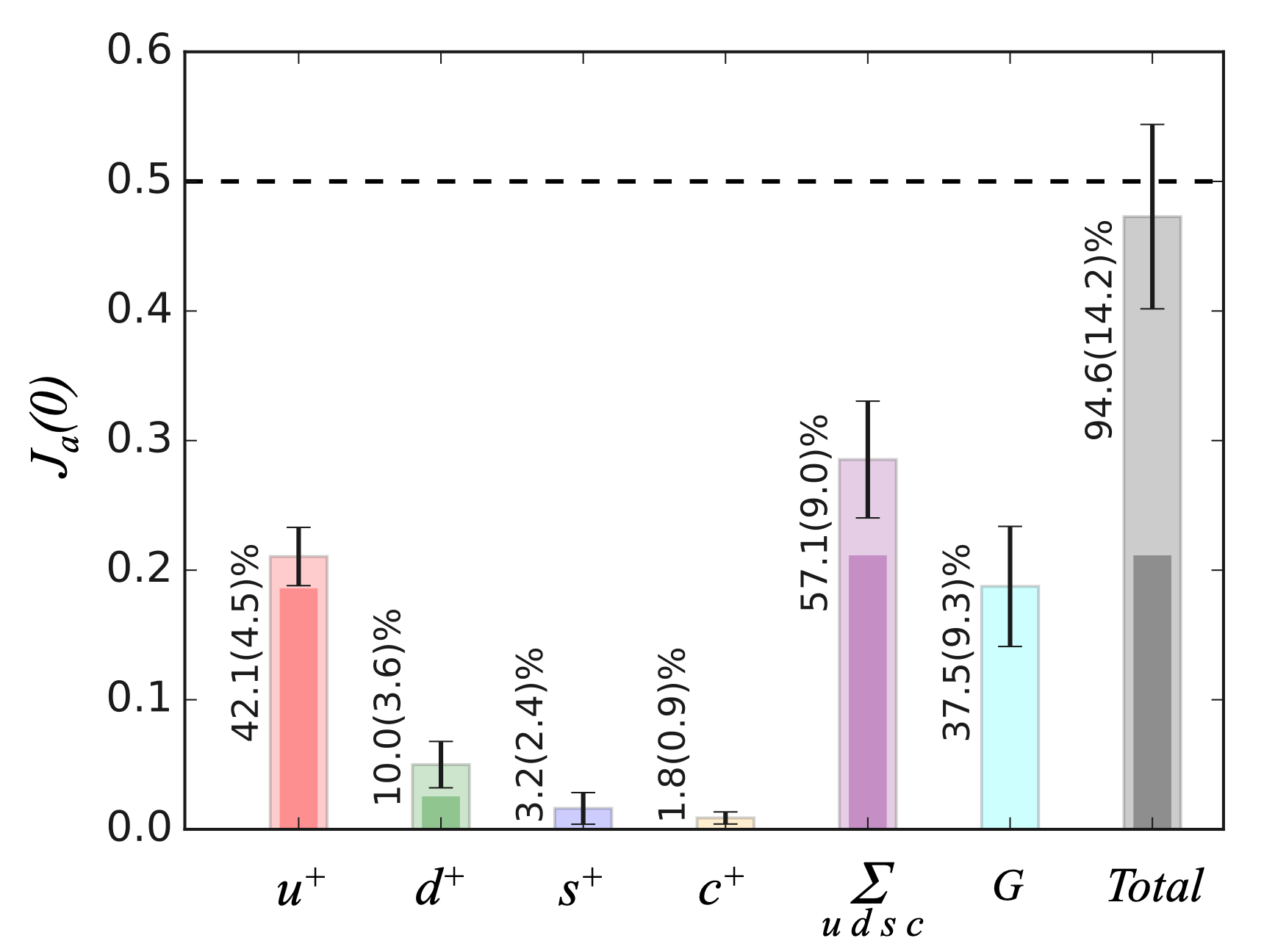
Figure 5: Proton spin decomposition computed in lattice QCD in  Alexandrou et al. (2020a), given in the $\overline{\text{MS}}$ scheme at 2 GeV. Each component includes the contribution of both the quarks and antiquarks ($q^{+}=q+\overline{q}$); outer/light (inner/dark) shaded bars denote the total (purely connected) contributions.

In the same vein, precise decompositions of the quark and gluon contributions to the proton’s momentum, which are related to the mass decomposition, have been achieved with complete systematic control in the same computational frameworks that yielded the spin decomposition Alexandrou et al. (2020a); Wang et al. (2022a). Contributions from the trace anomaly to the proton’s mass decomposition are more difficult to compute directly with systematic control, but have been constrained using the trace sum rule (20); Fig. 7 shows the first insight from lattice QCD into the pion mass (or quark mass) dependence of the proton’s mass decomposition Yang et al. (2018b). It is particularly notable that while the quark scalar condensate contribution varies rapidly with quark mass, the other contributions, including that of the trace anomaly, remain approximately constant.

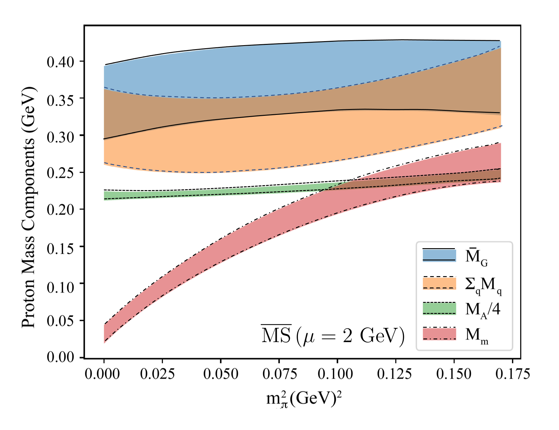
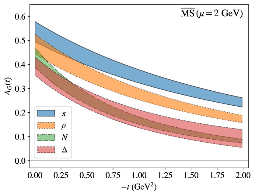
Figure 6: Ji’s mass decomposition (i.e. combination of (16) and (17)) for a proton computed in lattice QCD in Yang et al. (2018b) at a scale $\mu=2$ GeV, as a function of the pion mass.

Figure 7: $A_{G}(t)$ GFF for various hadrons from Pefkou et al. (2022), with quark masses corresponding to a larger-than-physical value of the pion mass of 450 MeV.

While local matrix elements in nuclear states can in principle be computed in lattice QCD in the same way as in the proton state, such calculations face significant practical and computational challenges, in particular compounding factorial and exponential growth in computational cost with the atomic number of the nuclear state. To date, a single first-principles calculation of isovector quark momentum fraction $A_{u-d}(0)$ in ${}^{3}\text{He}$ Detmold et al. (2021b) has been achieved; despite significant systematic uncertainties, including the result into global fits of experimental lepton-nucleus scattering data yields improved constraints on the nuclear parton distributions. Over the coming decade, it can be anticipated that the control and precision achieved in first-principles calculations of simple aspects of the gravitational structure of the proton will be extended to nuclear states.

Beyond forward-limit matrix elements, lattice QCD has also been used to compute the quark and gluon GFFs of the proton and other hadrons. Such calculations are computationally more demanding than those needed to constrain the forward-limit components, and statistical uncertainties increase with $|t|$. As a result, these studies have not yet achieved the same level of systematic control as the spin and mass decomposition. Nevertheless, the quark contributions to the proton’s GFFs (and those of other hadrons such as the pion) have been computed with $|t|\lesssim 1~{}\text{GeV}^{2}$ Bali et al. (2016); Brömmel et al. (2006); Brömmel (2007); Yang et al. (2018a); Alexandrou et al. (2018); Yang et al. (2018b); Alexandrou et al. (2017, 2020a, 2020c); Hägler et al. (2008). The gluon contributions to the proton’s GFFs are far less well-constrained, and almost all calculations to date have been performed with quark masses corresponding to larger-than-physical values of the pion mass Shanahan and Detmold (2019b, a); Pefkou et al. (2022); Detmold et al. (2017). Nevertheless, the gluon GFFs with $|t|\lesssim 2~{}\text{GeV}^{2}$ were computed for a range of hadrons in Pefkou et al. (2022), allowing qualitative comparisons of their $t$-dependence as illustrated in Fig. 7. Of particular recent interest has been the $D(t)$ GFF, which does not have a sum-rule constraint in the foward limit; a comparison between lattice QCD calculations of the quark and gluon contributions is illustrated in Fig. 8.

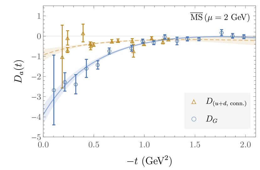
Figure 8: $D_{G}(t)$ and $D_{u+d}(t)$ GFF for the proton from Shanahan and Detmold (2019a) and Hägler et al. (2008) respectively, with quark masses corresponding to a pion mass of approximately 450 MeV.

In contrast to local matrix elements, matrix elements defined with light-cone separations, yielding e.g. the $x$-dependence of GPDs, can not be directly computed in Euclidean spacetime, but must be approached by indirect means. Significant developments over the last two decades have yielded a range of complementary approaches to direct calculations of GPDs themselves in the lattice QCD framework Detmold and Lin (2006); Ji (2013); Chambers et al. (2017); Ma and Qiu (2018); Radyushkin (2017); Constantinou et al. (2021); Detmold et al. (2021a). Given the significant technical and computational challenges of these approaches, the first lattice QCD studies of the $x$-dependence of the proton GPDs were achieved only recently in 2020 Alexandrou et al. (2020d); Lin (2021). Calculations with complete systematic control will require continued efforts over the coming years.

V Experimental results

This section presents a discussion of the DVCS data and the analysis procedure that led to the first extraction of the proton $D$-term form factor $D_{q}(t)$ from data collected with the CLAS detector at Jefferson Lab (JLab). The extraction of $D_{q}(t)$ of $\pi^{0}$ from Belle data, and other phenomenological results, are also reviewed.

V.1 DVCS in fixed-target and collider experiments

The first measurements of DVCS on unpolarized protons were carried out with the H1 Adloff et al. (2001) experiment and later with the ZEUS Chekanov et al. (2003)  experiment, both at the HERA collider. The first observation of the $\sin(\phi)$-dependence for the ${\vec{e}}p\rightarrow e^{\prime}p^{\prime}\gamma$ process as signature of the interference of the DVCS and Bethe-Heitler amplitudes came from the CLAS Stepanyan et al. (2001) and HERMES Airapetian et al. (2001) detectors.

These initial results triggered the development of a worldwide dedicated experimental program to measure the DVCS process with high precision and in a large kinematic range with HERMES at HERA, Hall A and CLAS at JLab, and COMPASS at CERN. A review of the early DVCS experiments can be found in d’Hose et al. (2016).

V.2 First extraction of the proton GFF $D_{q}(t)$

In this section, the data and procedure used in Burkert et al. (2018) to obtain the first determination of the quark contribution to the $D$-term of the proton are described. This work is based on two main pieces of experimental information from the CLAS detector at JLab Mecking et al. (2003), namely the beam-spin asymmetry (BSA) measured with spin-polarized electron beams, and the unpolarized cross section for DVCS on the proton.

The polarization asymmetries and differential cross sections have been used to extract the imaginary and real parts of the CFF ${\cal H}$ respectively. Using the dispersion relation technique to determine the subtraction term $\mathcal{C}_{\mathcal{H}}(t)$, as discussed in section III.1, requires the full integral over $0\leq\xi\leq 1$ at fixed $t$ to be evaluated. As this process requires an extrapolation to both $\xi=0$ and to $\xi=1$ that are unreachable in experiments, a parameterization of the $\xi$-dependence of Im$\mathcal{H}$ close to these limits has been incorporated to fit the data.

In the first step, fits of the BSA Girod et al. (2008) and of the unpolarized differential cross-sections Jo et al. (2015) for DVCS were performed to estimate Im${\mathcal{H}(\xi,t)}$ and Re${\mathcal{H}(\xi,t)}$ at fixed kinematics in $\xi$ and $t$ in the ranges covered by the data. The BSA is defined as

$$A_{LU}(\xi,t)=\frac{N^{+}(\xi,t)-N^{-}(\xi,t)}{N^{+}(\xi,t)+N^{-}(\xi,t)},$$ (35)

where $N^{+}$ and $N^{-}$ refer to the measured event rates at electron helicity $+1$ and $-1$, respectively.

The experimentally-measured BSA in $\vec{e}p\to ep\gamma$ contains not only the DVCS term, with the photon generated at the proton vertex, but also the Bethe-Heitler term with the photon generated at the incoming or scattered electron, respectively (see Fig. 2). Both have the same final state and thus interfere. They generate a $\sin\phi$-dependent interference contribution as seen in Fig. 9. The DVCS term is dominated by the CFF Im$\mathcal{H}$ and the Bethe-Heitler term is real and is given by the elastic electromagnetic FFs.

It is important to note that this analysis does not rely on extracted cross sections but on asymmetries of event rates in specific bins. This is an essential advantage as it avoids accounting for systematic uncertainties that must be included in the cross section extraction. The uncertainties in $A_{LU}(\xi,t)$ are dominated by statistics rather than systematic uncertainties, which determines the local values of Im$\mathcal{H}$ very precisely as can be seen in the top panel of Fig. 9, which shows the BSA and the differential cross sections for selected kinematic bins.

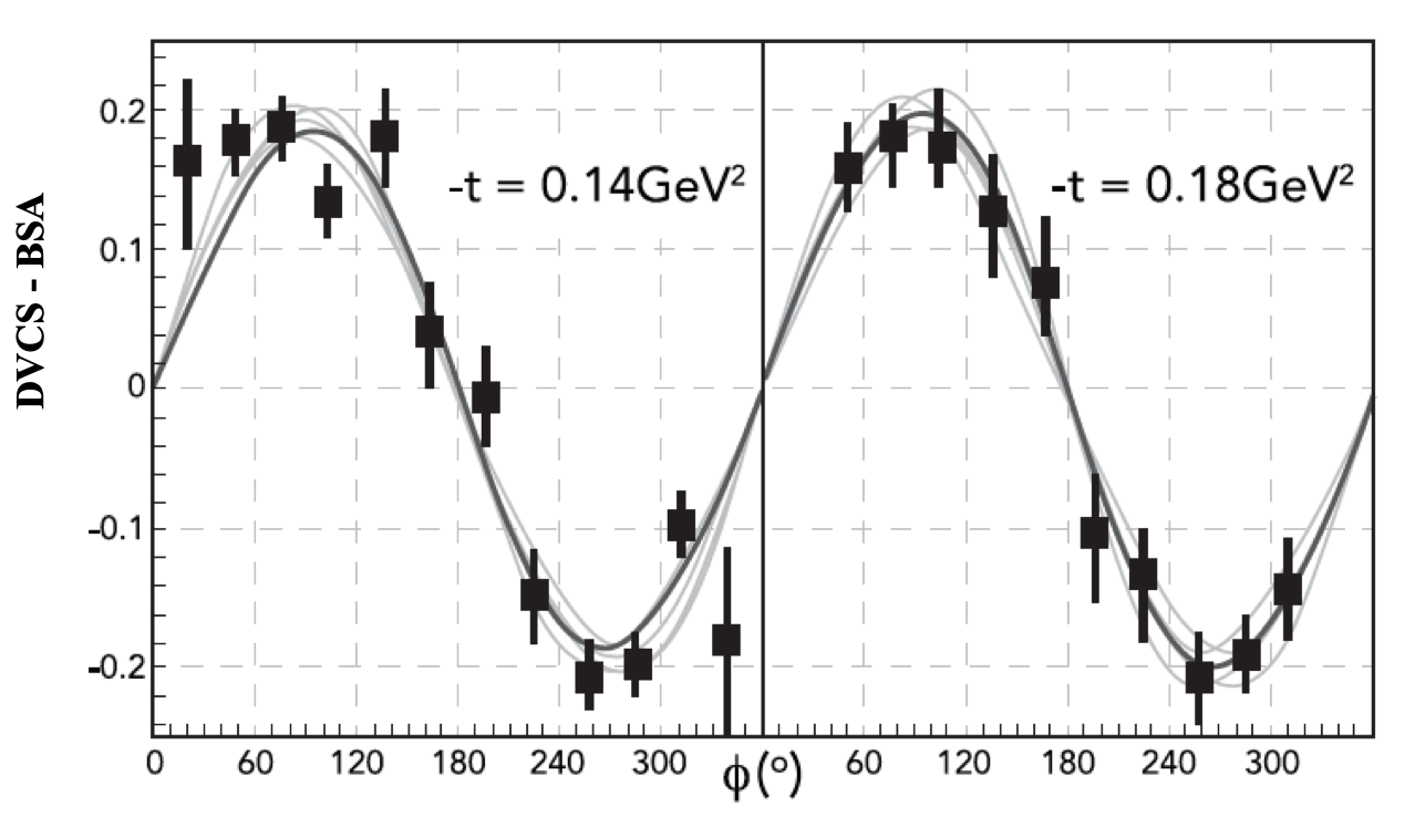
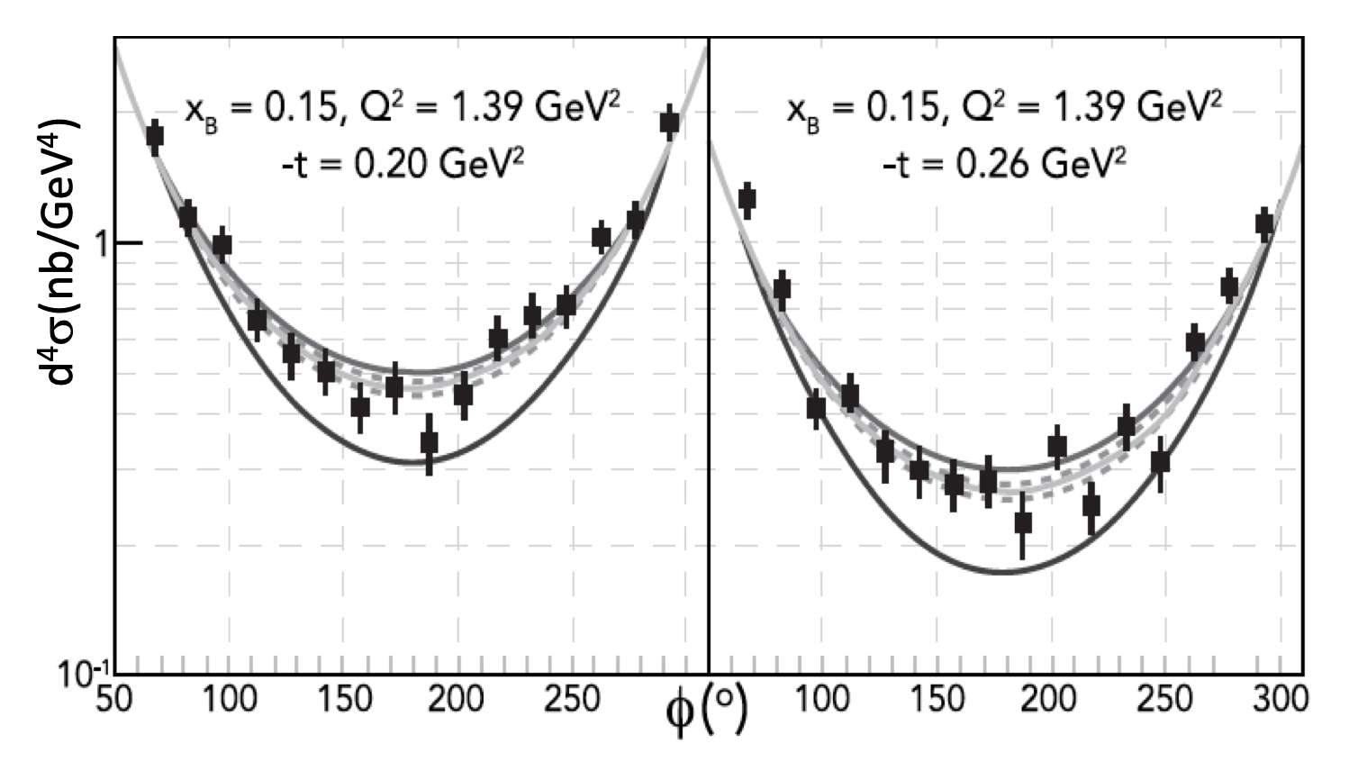
Figure 9: Top: The expected $\sin{\phi}$ dependence is fit to the data. The thick solid lines are the global fits using the parameterization according to (36). The bunch of thin solid lines represent local fits. The spread of the lines represent estimates of the systematic uncertainties. Bottom: The unpolarized cross section at fixed $\xi$ and $Q^{2}$ for different $t$ values. The azimuthal $\phi$ angle dependence of the cross section is fit to the experimental data. The thin dark solid line is the global fit. The upper thin gray lines represent fits at the given kinematics with the dashed lines showing the systematic uncertainties. The lower thick black lines show the Bethe-Heitler contributions. The graphics is adapted by permission from Burkert et al. (2018). Note the logarithmic vertical scale.

In the second step, the Im$\mathcal{H}(\xi,t)$ are fit with the functional form used in global fits Müller et al. (2014); Kumerički et al. (2016) with the parameters fit to the local CLAS data. The imaginary part is written as:

$${\textrm{Im}}\mathcal{H}(\xi,t)=\frac{\mathcal{N}}{1+\xi}\frac{\left(\frac{2\xi}{1+\xi}\right)^{-\alpha(t)}\left(\frac{1-\xi}{1+\xi}\right)^{b}}{\left(1-\frac{1-\xi}{1+\xi}\frac{t}{M^{2}}\right)^{p}},$$ (36)

where $\mathcal{N}$ is a free normalization constant, $\alpha(t)$ is fixed from small-$x$ Regge phenomenology as $\alpha(t)=0.43+0.85\,t~{}\text{GeV}^{-2}$, $b$ is a free parameter controlling the large-$x$ behavior, $p$ is fixed to 1 for the valence quarks, and $M$ is a free parameter controlling the $t$-dependence.

The real and imaginary part are fit together including the subtraction term in the dispersion relation (28). Fig. 10 compares the fits at fixed kinematics (local fits) with the global fit for one of the $t$ values. The global and local fits show good agreement in $\xi$ and $t$ kinematics where they overlap.

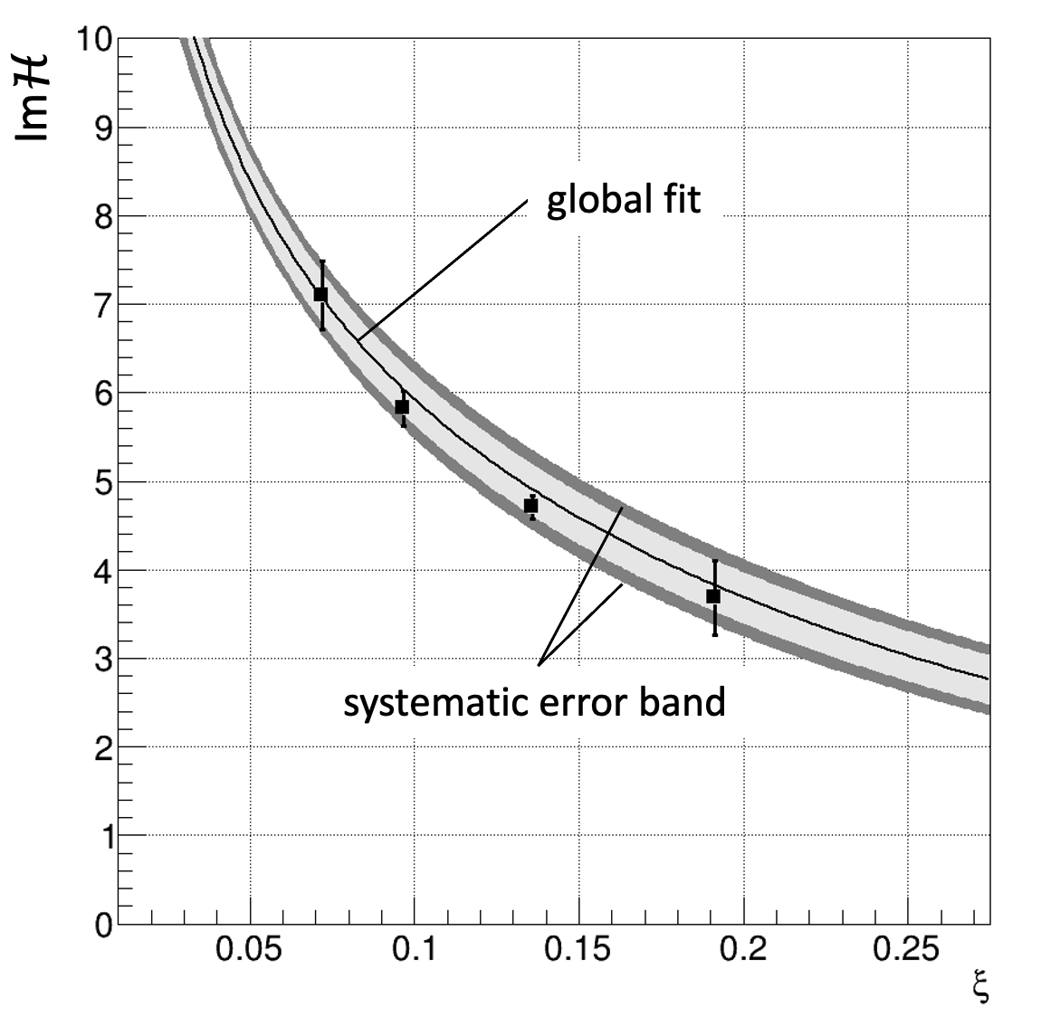
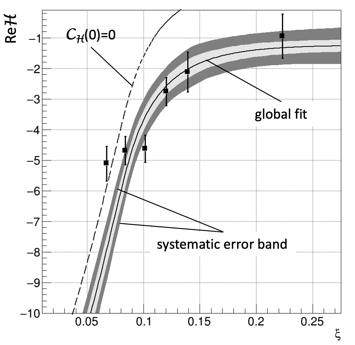
Figure 10: Top: The Im${\cal H}$ data points are plotted as function of $\xi$ from local fits to the $A_{LU}$ data Girod et al. (2008) for $-t=0.13$-$0.15$ GeV². The central solid line is the global fit constrained by the data points. The light gray error band is due to the uncertainty of the other CFFs. The outer dark-gray band shows the total systematic uncertainty to the imaginary part of the fit. Bottom: Re$\cal{H}$ data as extracted from unpolarized cross section data Jo et al. (2015). The central solid curve shows the result of the global fit with the dispersion relation applied and the fit parameters of the multipolar form for $\mathcal{C}_{\mathcal{H}}(t)$. The other lines/bands describe the same contribution as for Im${\cal H}$ propagated with the dispersion relation. The dashed line separated from the error bands shows the real part of the amplitude computed from the imaginary part using the dispersion relation and setting $\mathcal{C}_{\mathcal{H}}(0)$ to zero. The difference of dashed line and the solid line shows the effect of the subtraction term. Note that all markers in Re${\cal H}$ contribute to the precision of a single $-t$ value in $\mathcal{C}_{\mathcal{H}}(t)$, resulting in a small fit uncertainty.

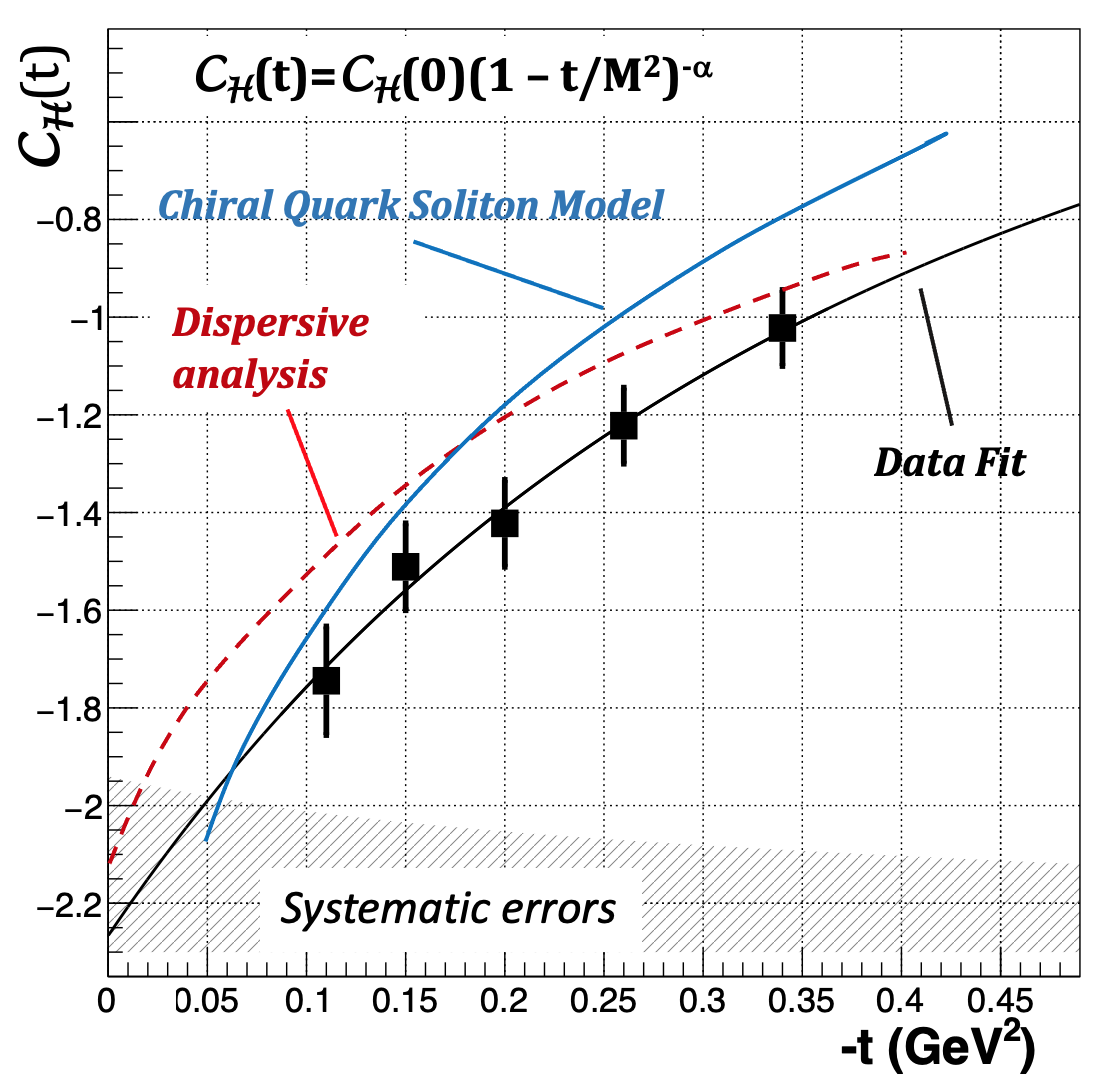
Figure 11: The subtraction term $\mathcal{C}_{\mathcal{H}}(t)$ as determined from the dispersion relation in the global fit (markers), adapted from Burkert et al. (2018). The uncertainties represent results of the fit errors. The hatched area at the bottom represents the estimated systematic uncertainties as described in Fig. 10 for one of the bins in $-t$. The dashed and solid-blue curves show the dispersive calculation Pasquini et al. (2014) and the chiral quark-soliton model predictions Goeke et al. (2007a), respectively.

In the fit, $\mathcal{C}_{\mathcal{H}}(t)$ is obtained at fixed $t$. The results for the subtraction term and the fit to the multipole form

$$\mathcal{C}_{\mathcal{H}}(t) = \mathcal{C}_{\mathcal{H}}(0)\bigg{[}1+\frac{(-t)}{M^{2}}\bigg{]}^{-\lambda}$$ (37)

are displayed in Fig. 11, where $\mathcal{C}_{\mathcal{H}}(0)$, $\lambda$ and $M^{2}$ are the fit parameters, with their values found to be:

$$\mathcal{C}_{\mathcal{H}}(0) =-2.27\pm 0.16\pm 0.36,$$ (38)

$$M^{2} =1.02\pm 0.13\pm 0.21{\rm~{}GeV^{2}},$$

$$\lambda =2.76\pm 0.23\pm 0.48.$$

The first error is the fit uncertainty, and the second error is due to the systematic uncertainties. Adding the fit errors for $\mathcal{C}_{\mathcal{H}}(0)$ and the systematic errors in quadrature $\sigma_{\mathcal{C}_{\mathcal{H}}(0)}=\sqrt{0.16^{2}+0.36^{2}}\approx 0.39$, the significance $S$ of the knowledge of the subtraction term is:

$$S=\frac{\mathcal{C}_{\mathcal{H}}(0)}{\sigma_{\mathcal{C}_{\mathcal{H}}(0)}}\approx 5.8.$$ (39)

More flexible analyses based on unconstrained artificial neural network techniques Kumerički (2019); Dutrieux et al. (2021) find however that a more conservative extraction of the subtraction constant from the currently available experimental data remains compatible with zero within large uncertainties.

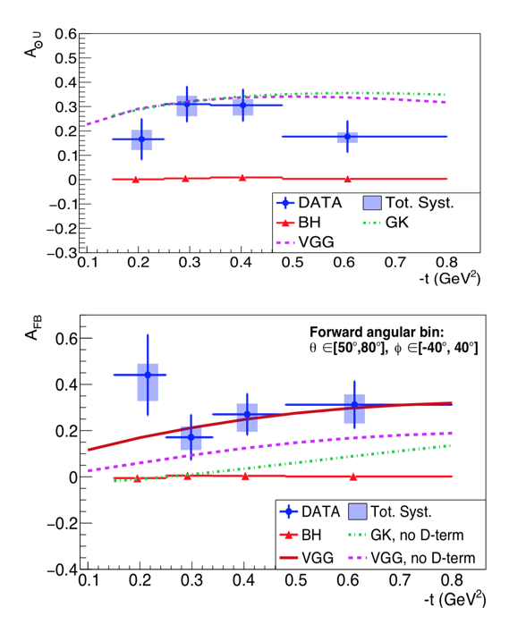
Figure 12: The TCS polarized BSA (top) and the TCS $A_{FB}$ (bottom) for an average 1.8 GeV mass of the time-like photon $M_{e^{+}e^{-}}$. A value for $A_{LU}$ of (20-25)% is consistent with what is measured in DVCS and projects out Im${\cal H}$. The FBA projects out Re${\cal H}$ that relates directly to the protons $D_{q}(t)$-term. Graphics adapted from  Chatagnon et al. (2021). The data require the presence of the $D$-term as seen in the difference of the dashed magenta line and the solid red line. At the kinematics of the data in Fig. 11, about half of the asymmetry may be due to the $D$-term when comparing calculations without and with the $D$-term Vanderhaeghen et al. (1999); Pasquini et al. (2014).

In the analysis of Burkert et al. (2018), the term $d_{3}^{q}(t)$ and other higher-order terms have been omitted in the expansion (30) to extract the GFF $D_{q}(t)$. The estimated effect is included in the systematic error analysis. It is also assumed that $u$ and $d$ quarks have the same first moments $d_{1}^{u}\approx d_{1}^{d}\approx{d_{1}^{u+d}/2}$, an assumption justified in the large-$N_{c}$ limit Goeke et al. (2001). Under these approximations, it follows from (31) that

$$\mathcal{C}_{\mathcal{H}}(t)\approx\frac{10}{9}\,d_{1}^{u+d}(t)=\frac{25}{18}\,D_{u+d}(t).$$ (40)

The truncation in (30) leads to a systematic uncertainty of a priori unknown magnitude. For $Q^{2}\to\infty$, the higher order terms $d^{q}_{3},d^{q}_{5},\cdots$ vanish. But at the $Q^{2}$ that can be reached in the current experiments, they are not necessarily negligible. The results of the chiral quark-soliton model, which predicts values of $d^{u+d}_{1}$ close to findings in the experimental analysis Goeke et al. (2007a), can been used to estimate the contribution of the $d_{3}^{q}$ term. At the kinematics relevant for this analysis a ratio $d^{u+d}_{3}/d^{u+d}_{1}\approx 0.3$ was found Kivel et al. (2001). A systematic uncertainty of $\delta(d^{u+d}_{1})/d^{u+d}_{1}=\pm 0.30$ has therefore been included into the results of Burkert et al. (2018) for $d_{1}^{u+d}(t)$.

One may ask if the first two terms in the Gegenbauer polynomial expansion $d_{1}^{q}(t)$ and $d_{3}^{q}(t)$ could be separated in some way to reduce the systematics. This has been studied in Dutrieux et al. (2021) by including the $Q^{2}$-evolution into the phenomenological analysis. It was found that, assuming the same $t$-dependence, the two terms cannot currently be separated given the limited range in $Q^{2}$ covered by the data. In the future one may expect Lattice QCD to be able to provide a model-independent evaluation of this higher-order contribution.

To conclude this section, the determination of $\mathcal{C}_{\mathcal{H}}(t)$ suggests that the quark contribution $\sum_{q}D_{q}(t)$ to the proton’s GFF $D(t)$ is non-zero and large. These results have been supported in a recent paper on the first measurement of TCS Chatagnon et al. (2021) as shown in Fig. 12, where the contribution of the $D$-term to the forward-backward asymmetry is seen to be significant. Moreover, predictions in the chiral quark-soliton model Goeke et al. (2007a) and from dispersive analysis Pasquini et al. (2014) shown in Fig. 11 are consistent with the results discussed here within the systematic uncertainties.

V.3 Other measurements and phenomenological studies

The first extraction of the $\pi^{0}$ GFFs in the time-like region based on the process $\gamma\gamma^{*}\to\pi^{0}\pi^{0}$, depicted in Fig. 3, which was measured in the Belle experiment in $e^{+}e^{-}$ collisions Masuda et al. (2016), was obtained in Kumano et al. (2018). For the quark contribution to the $\pi^{0}$ $D$-term the value $\sum_{q}D_{q}(0)\approx-0.75$ was reported, but systematic uncertainties have not been estimated. It has recently been observed in Lorcé et al. (2022a) that kinematical corrections may significantly impact the extraction of generalized distribution amplitudes from experimental data and should be taken into account in future analyses.

Based on data from experiments at JLab on the energy-dependence of $J/\Psi$ production at threshold Ali et al. (2019); Duran et al. (2023), phenomenological information on the gluon $D_{G}(t)$ form factor of the proton was extracted Kharzeev (2021); Kou et al. (2021); Wang et al. (2022b) and estimates were obtained for the gluon contributions to the proton mean square mass radius $\int\mathrm{d}^{3}r\,r^{2}\mathcal{T}^{00}(\vec{r})/M_{N}$ and the mean square scalar radius $\int\mathrm{d}^{3}r\,r^{2}g_{\mu\nu}\mathcal{T}^{\mu\nu}(\vec{r})/M_{N}$. The most recent data on this process were reported in Adhikari et al. (2023). (For remarks on the theoretical status of this process see Sec. III.5.) A similar study for the lighter $\phi$-meson was presented in Hatta and Strikman (2021).

V.4 Future experimental developments to access GFFs

As discussed in section III, measurements of DVCS have so far been most effective in obtaining information related to GPDs. However, there are different experimental processes that may be employed to provide additional, or independent, information on the GPDs and GFFs.

Implementation of a high-duty-cycle positron source, both polarized and unpolarized Abbott et al. (2016), at JLab would significantly enhance its capabilities in the extraction of the CFF Re$\mathcal{H}(\xi,t)$ and thus of the gravitational form factor $D_{q}(t)$ and of the mechanical properties of the proton.

The time-like Compton scattering process will be measured in parallel to the DVCS process employing the large acceptance detector systems such as CLAS12 Burkert et al. (2020). The TCS event rate is much reduced compared to DVCS and requires higher luminosity for similar sensitivity to $\mathcal{H}$. In experiments employing large acceptance detector systems, both the DVCS and TCS processes are measured simultaneously, in quasi-real photo-production at very small $Q^{2}\to 0$, and in real photo-production, where the external production target acts as a radiator of real photons that undergo TCS further downstream in the same target cell.

The double DVCS process enables access to GPDs in their full kinematic dependencies on $x,\xi,t$, see Sec. III. At the same time it is reduced in rate by orders of magnitude compared to DVCS Kopeliovich et al. (2010) requiring higher luminosity than is currently achievable. Nevertheless, special equipment that would comply with such requirements has been proposed Chen et al. (2014). Such measurements are currently planned at JLab in Hall A and Hall B.

Finally, an energy-doubling of the existing electron accelerator at JLab is currently under consideration Arrington et al. (2022). This upgrade would extend the DVCS program to higher $Q^{2}$ and lower $x_{B}$ and better link the DVCS measurements at the current 12 GeV operation to the kinematic reach that will be available at the Electron-Ion Collider, a flagship future facility in preparation at the Brookhaven National Laboratory (discussed further below). It will also more fully open the charm sector to access the gluon GFFs.

VI Interpretation

In section II various properties of the GFFs have been discussed at zero momentum transfer. Much of the recent interest in GFFs comes from the fact that they contain information on the spatial distributions of energy, angular momentum, and internal forces that can be accessed at non-zero momentum transfer $t$, via an appealing interpretation which is reviewed here.

VI.1 The static EMT

The 3D interpretation Polyakov (2003) in Eq. (10) of the information encoded by GFFs provides analogies to intuitive concepts such as pressure. A 2D interpretation can also be carried out in other frames Lorcé et al. (2019); Freese and Miller (2021, 2022) with Abel transformations allowing one to relate 2D and 3D interpretations Panteleeva and Polyakov (2021).

Considering 2D EMT distributions for a nucleon state boosted to the infinite-momentum frame has the advantage that in this case the nucleon can be perfectly localized around the transverse center of momentum Burkardt (2000). In other frames or in 3D, an exact probabilistic parton density interpretation does not hold in general. The reservations are analogous to those in the case of, e.g., the interpretation of the electric FF in terms of a 3D electrostatic charge distribution (and the definition of electric mean square charge radius which, despite all caveats, remains a popular concept, giving an idea of the proton’s size). The 3D EMT description is nevertheless mathematically rigorous Polyakov and Schweitzer (2018b) and can be interpreted in terms of quasi-probabilistic distributions from a phase-space point of view Lorcé et al. (2019); Lorcé (2020). A strict probabilistic interpretation is, however, justified for heavy nuclei and for the nucleon in the large-$N_{c}$ limit, where recoil effects can be safely neglected Polyakov (2003); Goeke et al. (2007a); Polyakov and Schweitzer (2018b); Lorcé et al. (2022b).

The meaning of the different components of the static EMT is intuitively clear, with $\mathcal{T}^{00}(\vec{r})$ denoting the energy distribution and $\mathcal{T}^{0k}(\vec{r})$ representing the spatial distribution of momentum. In the following sections the focus is on $\mathcal{T}^{ij}(\vec{r})$ which are perhaps the most interesting components of the static EMT, thanks to their relation to the stress tensor and the $D$-term.

VI.2 The stress tensor and the $D$-term

The key to the mechanical properties of the proton is the symmetric stress tensor $\mathcal{T}^{ij}(\vec{r})$ given by Polyakov (2003)

$$\mathcal{T}^{ij}(\vec{r})=\biggl{(}\frac{r^{i}r^{j}}{r^{2}}-\frac{1}{3}\,\delta^{ij}\biggr{)}\,s(r)+\delta^{ij}\,p(r)\,$$ (41)

with $s(r)$ known as the shear force (or anisotropic stress) and $p(r)$ as the pressure with $r=|\vec{r}|$. Both are connected by the differential equation $\frac{2}{3}\,\frac{\mathrm{d}}{\mathrm{d}r}s(r)+\frac{2}{r}\,s(r)+\frac{\mathrm{d}}{\mathrm{d}r}p(r)=0$ and $p(r)$ obeys $\int_{0}^{\infty}\mathrm{d}r\,r^{2}p(r)=0$ von Laue (1911), a necessary but not sufficient condition for stability. These relations originate from the EMT conservation expressed by $\nabla^{i}\mathcal{T}^{ij}(\vec{r})=0$ for the static EMT. The total $D$-term $D(0)$ can be expressed in terms of $p(r)$ and $s(r)$ in two equivalent ways,

$$D(0)=-\frac{4}{15}\,M_{N}\!\!\int{\mathrm{d}^{3}r}\,r^{2}s(r)=M_{N}\!\!\int{\mathrm{d}^{3}r}\,r^{2}p(r)\,.\;\;\;\;\;$$ (42)

The form of the stress tensor (41) is valid for spin-0 and spin-$\frac{1}{2}$ hadrons; for higher spins see Cosyn et al. (2019); Polyakov and Sun (2019); Cotogno et al. (2020); Kim and Sun (2021); Ji and Liu (2021).

If the GFF $D(t)$ is known, then $s(r)$ and $p(r)$ are obtained as follows Polyakov and Schweitzer (2018b)

$$s(r) = -\frac{1}{4M_{N}}\,r\,\frac{\mathrm{d}}{\mathrm{d}r}\frac{1}{r}\frac{\mathrm{d}}{\mathrm{d}r}\widetilde{D}(r),$$ (43)

$$p(r) = \frac{1}{6M_{N}}\frac{1}{r^{2}}\frac{\mathrm{d}}{\mathrm{d}r}r^{2}\frac{\mathrm{d}}{\mathrm{d}r}\widetilde{D}(r),$$ (44)

where $\widetilde{D}(r)=\int\frac{\mathrm{d}^{3}\Delta}{(2\pi)^{3}}\,e^{-i{\vec{\Delta}\cdot\vec{r}}}D(-{\vec{\Delta}}^{2})$. If the separate $D_{q}(t)$ and $D_{G}(t)$ GFFs are known, “partial” quark and gluon shear forces $s_{q}(r)$ and $s_{G}(r)$ can be defined in analogy to (43). In order to define “partial” quark and gluon pressures, in addition to $D_{q}(t)$ and $D_{G}(t)$ knowledge of $\bar{C}_{q}(t)=-\bar{C}_{G}(t)$ is required. The latter are responsible for “reshuffling” forces between the gluon and quark subsystems inside the proton Lorcé (2018a); Polyakov and Son (2018) and are difficult to access experimentally. $\bar{C}_{q}(t)$ was studied in the bag model Ji et al. (1997), chiral quark-soliton model Goeke et al. (2007a), instanton vacuum model Polyakov and Son (2018) and lattice QCD Liu (2021). Estimates guided by renormalization group methods Hatta et al. (2018); Tanaka (2019); Ahmed et al. (2023) yield $\bar{C}_{q}(0)=-0.163(3)$ at $\mu=2\,{\rm GeV}$ in $\overline{\text{MS}}$ scheme Tanaka (2023).

VI.3 Normal forces and the sign of the $D$-term

The stress tensor $\mathcal{T}^{ij}(\vec{r})$ can be diagonalized, with one eigenvalue given by the normal force per unit area $p_{n}(r)=\frac{2}{3}\,s(r)+p(r)$ with the pertinent eigenvector $\vec{e}_{r}$. The other two eigenvalues are degenerate (for spin-0 and spin-$\frac{1}{2}$) and are known as tangential forces per unit area, $p_{t}(r)=-\,\frac{1}{3}\,s(r)+p(r)$, with eigenvectors which can be chosen to be unit vectors in the $\vartheta$- and $\varphi$-directions in spherical coordinates Polyakov and Schweitzer (2018b).

The normal force appears when considering the force $F^{i}=\mathcal{T}^{ij}\mathrm{d}S^{j}=p_{n}(r)\,\mathrm{d}S\,e_{r}^{i}=[\frac{2}{3}\,s(r)+p(r)]\,\mathrm{d}S\,e_{r}^{i}$ acting on a radial area element $\mathrm{d}S^{j}=\mathrm{d}S\,e_{r}^{j}$, where $e_{r}^{j}=r^{j}/r$. General mechanical stability arguments require this force to be directed towards the outside, or else the system would implode. This implies that the normal force per unit area must be positive

$$p_{n}(r)=\frac{2}{3}\,s(r)+p(r)>0\,.$$ (45)

As an immediate consequence of (45) one concludes by means of Eq. (42) that Perevalova et al. (2016)

$$D(0)<0\,.$$ (46)

For hadronic systems like protons, hyperons, mesons or nuclei for which the $D$-term has been computed (in models, chiral perturbation theory, lattice QCD or by dispersive techniques, see Sec. IV) or inferred from experiment (in the case of the proton and $\pi^{0}$, see Sec. V) it has always been found to be negative in agreement with (46).

The above definitions and conclusions are more than just a fruitful analogy to mechanical systems. At this point it is instructive to recall how one calculates the radii of neutron stars, which are amenable to an unambiguous 3D interpretation. In these macroscopic hadronic systems, general relativity effects cannot be neglected and are incorporated in the Tolman-Oppenheimer-Volkoff equation, which is solved by adopting a model for the nuclear matter equation of state. The solution yields (in our notation) $p_{n}(r)$ inside the neutron star as function of the distance $r$ from the center. The obtained solution is positive in the center and decreases monotonically until it drops to zero at some $r=R_{\ast}$, and would be negative for $r>R_{\ast}$ corresponding to a mechanical instability. This is avoided and a stable solution is obtained by defining $r=R_{\ast}$ to be the radius of the neutron star, see for instance Prakash et al. (2001). Thus, the point where the normal force per unit area drops to zero coincides with the “edge” of the system.

The proton has of course no sharp “edge”, being surrounded by a “pion cloud” due to which the normal force does not drop literally to zero but exhibits a Yukawa-type suppression at large $r$ proportional to $\frac{1}{r^{6}}\,e^{-2m_{\pi}r}$ Goeke et al. (2007a). In the less realistic but very instructive bag model, there is an “edge” at the bag boundary, where $p_{n}(r)$ drops to zero Neubelt et al. (2020). In contrast to the neutron star one does not determine the “edge” of the bag model in this way. Rather the normal force drops “automatically” to zero at the bag radius which reflects the fact that from the very beginning the bag model was constructed as a simple but mechanically stable model of hadrons Chodos et al. (1974).

VI.4 The mechanical radius of the proton and neutron

The “size” of the proton is commonly defined through the electric charge distribution which is indeed a useful concept, though only for charged hadrons. For an electrically neutral hadron like the neutron, the particle size cannot be inferred in this way. In that case, one may still define an electric mean square charge radius $r_{\rm ch}^{2}=6\,G^{\prime}_{E}(0)$ in terms of the derivative of the electric FF $G_{E}(t)$ at $t=0$. But for the neutron $r_{\rm ch}^{2}<0$ which gives insights about the distribution of electric charge inside neutron, but not about its size. This is ultimately due to the neutron’s charge distribution not being positive definite.

The positive-definite normal force per unit area,  (45), is an ideal quantity to define the size of the nucleon. One can define the mechanical radius as Polyakov and Schweitzer (2018a, b)

$$r_{\rm mech}^{2}=\frac{\int\mathrm{d}^{3}r\,r^{2}\,p_{n}(r)}{\int\mathrm{d}^{3}r\,p_{n}(r)}=\frac{6D(0)}{\int_{-\infty}^{0}\mathrm{d}t\,D(t)}\,.$$ (47)

Interestingly, this is an “anti-derivative” of a GFF as compared to the electric mean square charge radius defined in terms of the derivative of the electric FF at $t=0$. With this definition, the proton and neutron have the same radius (modulo isospin violating effects). Notice also that the (isovector) electric mean square charge radius diverges in the chiral limit and is therefore inadequate to define the proton size in that case, while the mechanical radius in (47) remains finite in the chiral limit Polyakov and Schweitzer (2018b). The mechanical radius of the proton is predicted to be somewhat smaller than its charge radius in soliton models Goeke et al. (2007a); Cebulla et al. (2007). The charge and mechanical radii become equal in the non-relativistic limit which was derived in the bag model Neubelt et al. (2020); Lorcé et al. (2022b).

VI.5 First visualization of forces from experiment

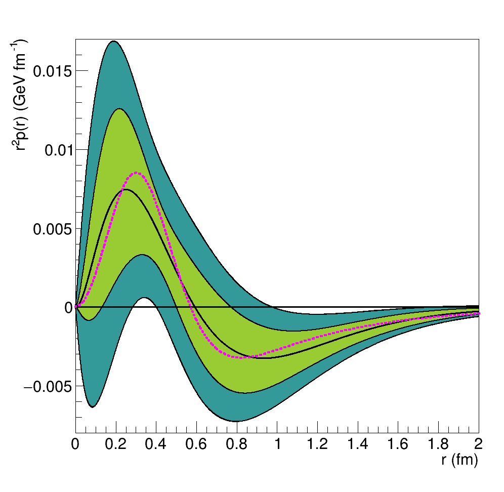
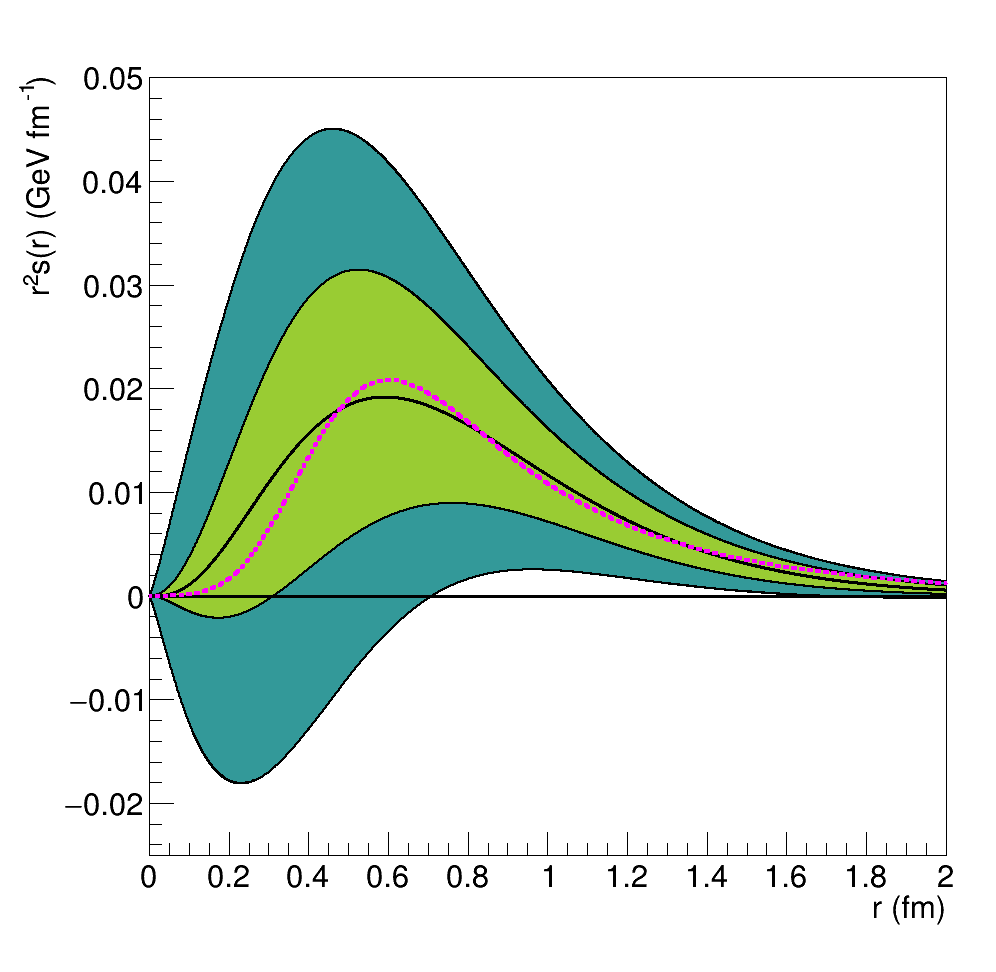
Figure 13: The distributions of pressure $r^{2}p_{q}(r)$ (top) and shear stress $r^{2}s_{q}(r)$ (bottom) on quarks in the proton based on JLab data Burkert et al. (2018, 2021b). The central solid lines show the best fit. The outer shaded areas mark the uncertainties when only data prior to the CLAS data are included. The inner shaded areas represent the uncertainties when the CLAS data are used. The widths of the bands are dominated by systematic uncertainties [which include extrapolation in unmeasured $\xi$-region when evaluating (28) and the neglect of higher-order terms in the Gegenbauer expansion described in (40)]. The dotted magenta curves represent the model predictions of Goeke et al. (2007a).

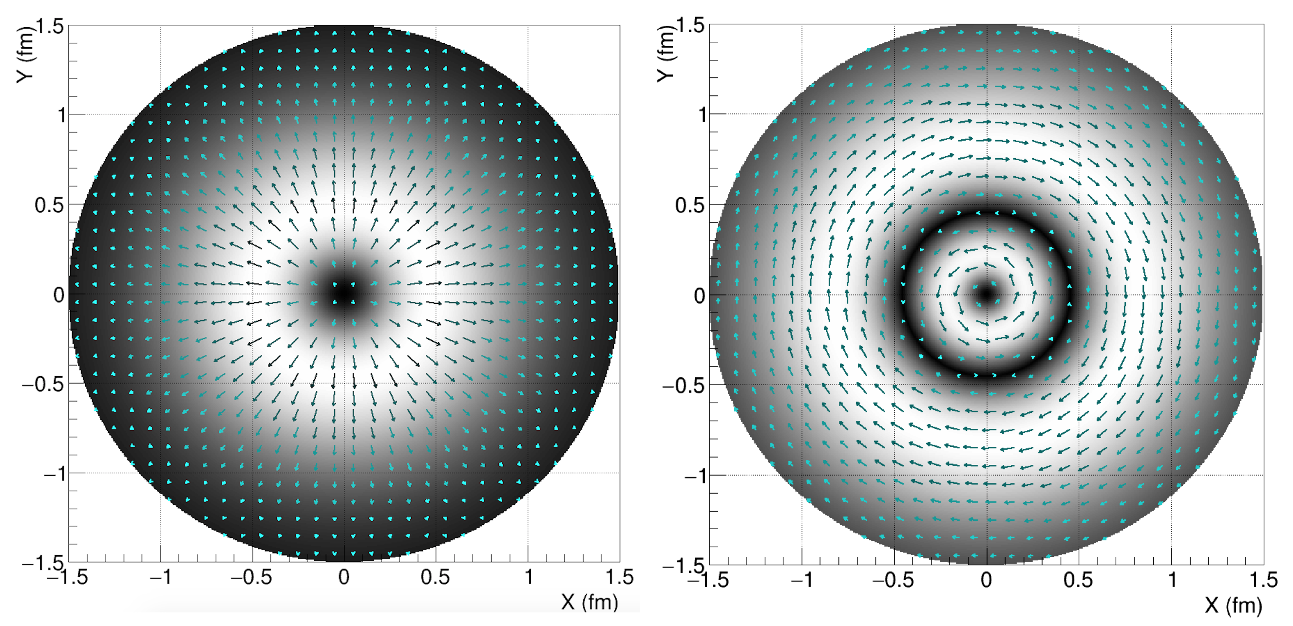
Figure 14: 2D display of the quark contribution to the distribution of forces in the proton as a function of the distance from the proton’s center Burkert et al. (2021b). The light gray shading and longer arrows indicate areas of stronger forces, the dark shading and shorter arrows indicate areas of weaker forces. Left panel: Normal forces as a function of distance from the center. The arrows change magnitude and point always radially outwards. Right panel: Tangential forces as a function of distance from the center. The forces change direction and magnitude as indicated by the direction and lengths of the arrows. They change sign near 0.4 fm from the proton center.

The first visualization of the force distributions in the proton was presented in Burkert et al. (2018) which will be reviewed here. As detailed in Sec. V.2, the DVCS data from JLab experiments Girod et al. (2008); Jo et al. (2015) provided information on the observable $\mathcal{C}_{\mathcal{H}}(t)$ in (28), from which, under certain reasonable (at present necessary) assumptions, information about the quark contribution $D_{u+d}(t)$ of the proton was deduced. Based on this information, (44) yields the results for the pressure $p_{q}(r)$ and the shear force $s_{q}(r)$ of quarks displayed in Fig. 13 (the index $q$ denotes here $u+d$ quark contributions, with heavier quarks neglected). In order to obtain $p_{q}(r)$, the additional assumption was made that $\bar{C}_{q}(t)$ can be neglected.

The $r^{2}p_{q}(r)$ distribution is positive, peaks near $0.25\,$fm, changes sign near $0.6\,$fm, and reaches its minimum value around 1.0 fm. The peak value of $r^{2}s_{q}(r)$ is around $20$ MeV fm^-1, and occurs near $0.6\,$fm from the proton’s center, where the shear force, given by $4\pi r^{2}s_{q}(r)$, reaches $240$ MeV fm^-1 or $38$ kN, an appreciably strong force inside the tiny proton. It is interesting to observe that these results are consistent with predictions from the chiral quark-soliton model Goeke et al. (2007a) within the (large) systematic uncertainties in the data.

The quark contribution to the normal and tangential forces, $p_{n,q}$ and $p_{t,q}(r)$ as defined in Sec. VI.3, are displayed in a two-dimensional plot in Fig. 14. This figure shows the 3D distributions inside the proton in a slice going through the “equatorial plane”. The normal forces are strongest at mid-distances near $0.5\,$fm from the proton center and drop towards the center and towards the outer periphery. The tangential forces exhibit a node near $0.40\,$fm from the center.

VI.6 The $D$-term and long-range forces

Among the open questions in theory is the issue of how to define the $D$-term in the presence of long-range forces. It was shown in a classical model of the proton Białynicki-Birula (1993) that $D(t)$ diverges like $1/\sqrt{-t}$ for $t\to 0$ due to the $\frac{1}{r}$-behavior of the Coulomb potential Varma and Schweitzer (2020). This result is model-independent and was found also for charged pions in chiral perturbation theory Kubis and Meissner (2000), in calculations of quantum corrections to the Reissner-Nordström and Kerr-Newman metrics Donoghue et al. (2002), and for the electron in QED Metz et al. (2021).

The deeper reason why $D(t)$ diverges for $t\to 0$ due to QED effects might be ultimately related to the presence of a massless physical state (the photon) which has profound consequences in a theory. Notice that $D(t)$ is the only GFF which exhibits this feature when QED effects are included. There are two reasons for this. First, the other proton GFFs are constrained at $t=0$, see (5) and (6), while $D(t)$ is not. Second, $D(t)$ is the GFF most sensitive to forces in a system Hudson and Schweitzer (2017). Notice that $D(t)$ is multiplied by the prefactor $(\Delta^{\mu}\Delta^{\nu}-g^{\mu\nu}\Delta^{2})$ such that despite the divergence of $D(t)$ due to QED effects the matrix element $\langle p^{\prime}|T_{a}^{\mu\nu}|p\rangle$ is well-behaved in the forward limit.

There have been studies of the $D$-term for the H-atom Ji and Liu (2021, 2022), which defy the interpretation presented here. This is perhaps not a surprise considering the differences between hadronic and atomic bound states. Atoms are comparatively large, low-density objects. Pressure concepts from continuum mechanics might not apply to atoms whose stability is well-understood within non-relativistic quantum mechanics. In contrast to this, the proton as a QCD bound state has nearly the same mass as an H-atom but a much smaller size $\sim 10^{-15}$m and constitutes a compact high-density system (15 orders of magnitude more dense than an atom) where continuum mechanics concepts may be applied and provide insightful interpretations. Another important aspect might be played by the role of confinement absent for atoms which can be easily ionized. Hadrons constitute a much different type of bound state in this respect. More theoretical work is needed to clarify these issues.

VII Summary and outlook

This Colloquium gives an overview of the exciting recent developments along a new avenue of experimental and theoretical studies of the gravitational structure of hadrons, especially the proton.

The gravitational form factors of the proton rose to prominence after the works of Xiangdong Ji Ji (1995a, 1997b) illustrated how they can be used to gain insight into fundamental questions such as: how much do quarks and gluons contribute to the mass and the spin of the proton? Soon afterwards, Maxim Polyakov Polyakov (2003) showed that they also provide information about the spatial distribution of mass and spin, and allow one to study the forces at play in the bound system. These works triggered many follow-up studies and investigations which have deepened our understanding of proton structure.

Through matrix elements of the energy-momentum operator, the gravitational form factors of the proton and other hadrons have been studied in theoretical approaches including a wide range of models and in numerical calculations in the framework of lattice QCD. In broad terms, the simplest aspects of the EMT structure of the proton and other hadrons (such as the pion) have been understood from theory for some number of years, and first-principles calculations providing complete and controlled decompositions of the proton’s mass and spin, for example, are now available. On the other hand, more complicated aspects of proton and nuclear structure, such as gluon gravitational form factors, the $x$-dependence of generalized parton distributions, and energy-momentum tensor matrix elements in light nuclei, have been computed for the first time in the last several years, as yet without complete systematic control, and significant progress can yet be expected over the next decade. Theory insight into these fundamental aspects of proton and nuclear structure is thus currently in a phase of rapid progress, complementing the improvement of experimental constraints on these quantities and, importantly, providing predictions which inform the target kinematics for future experiments.

The first experimental results, discussed in this colloquium, are based on precise measurements of the deeply virtual Compton scattering process with polarized electron beam, that determined both, the beam-spin asymmetry and the absolute differential cross section of $\vec{e}p\to ep\gamma$. Measurements covered a limited range in the kinematic variables which made it necessary to employ information from high-energy collider data to constrain the global data fit in the region that was not covered in the CLAS experiment. Consequently, large systematic uncertainties were assigned to the results.

New experimental results on DVCS measurements with polarized electron beams at higher energy have recently been published from experiments with CLAS12 Christiaens et al. (2022) and from Hall A at Jefferson Laboratory Georges et al. (2022). They extend the kinematic reach both to higher and to lower values in $\xi$, and increase the range covered in $Q^{2}$. The latter will allow for more sensitive measurements of the $Q^{2}$ evolution of the DVCS cross section. These new data may also support application of machine learning techniques and artificial neural networks in the higher level data analysis as have been developed by several groups Kumerički (2019); Berthou et al. (2018); Grigsby et al. (2021).

Ongoing experiments and future planned measurements that employ proton and deuterium (neutron) targets, spin-polarized transversely to the beam direction, have strong sensitivity to CFF $\mathcal{E}$. Precise knowledge of the kinematic dependence of $\mathcal{E}(\xi,t)$ is needed to measure the quark angular momentum distribution encoded in the GFF $J_{q}(t)$ of the proton Ji (1997b), as defined in Sect. II.1.

The plan to extend the Jefferson Lab’s electron accelerator energy reach to 22 GeV would more fully open access to employing $J/\Psi$ production near threshold in a wide $t$ range, and some $\xi$ range to access the gluon part $D_{G}(t)$ of the proton’s $D$-term.

DVCS data from the COMPASS experiment at CERN with 160 GeV of oppositely polarized $\mu^{+}$ and $\mu^{-}$ beams Akhunzyanov et al. (2019) reach to smaller $\xi$ values and into the sea-quark region. The average of the measured $\mu^{+}$ and $\mu^{-}$ cross sections allows for the determination of Im$\cal{H}$. Results from high statistics runs that cover the lower $x_{B}$ domain are expected in the near future. With these new data, the difference of $\mu^{+}$ and $\mu^{-}$ cross sections can also be formed to obtain the charge asymmetry, which provides direct access to Re$\cal{H}$.

A long term perspective is provided by the planned Electron-Ion Collider projects in the US Abdul Khalek et al. (2022); Burkert et al. (2023) and in China Anderle et al. (2021). The US project will extend the kinematic reach in $x_{B}>10^{-4}$ and thus will cover with high operational luminosity up to $10^{34}\,\text{cm}^{-2}\,\text{s}^{-1}$ the gluon dominated domain. It features polarized electron and polarized proton beams, the latter longitudinally or transversely polarized, and light ion beams. The EIcC in China focuses on the lower energy domain with $x_{B}>10^{-3}$ that connects more closely to the kinematics of the fixed target experiments at Jlab that operate at very high luminosity in the valence quark and the $q\bar{q}$-sea domain.

Currently available data allowed for a pioneering first step into this emerging new field of the proton internal structure, complementing what has been learned in many detailed experiments over the past 70 years of studies of the proton electromagnetic structure, with the first result on the proton’s mechanical structure.

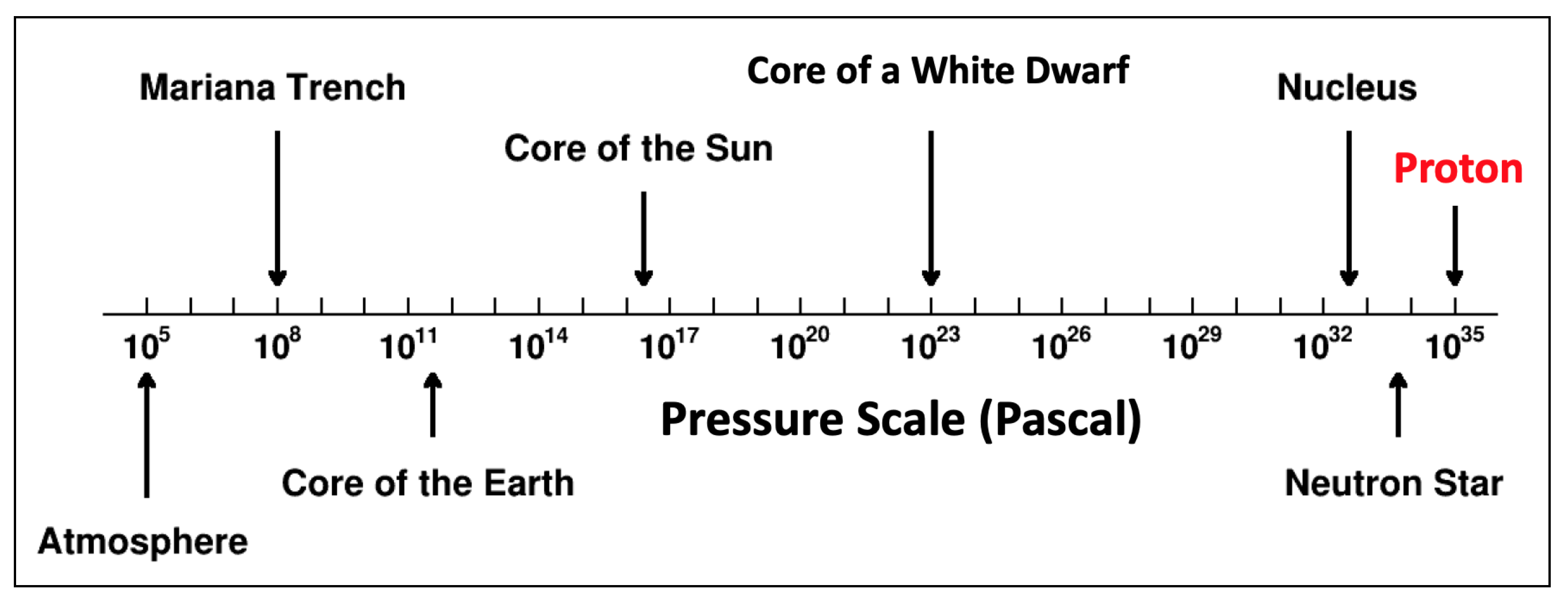
Figure 15: Comparison of peak pressures inside various objects on earth, in the solar system, and in the universe.

This new avenue of research has been rapidly developing theoretically, and the first experimental results on the proton firmly established the study of mechanical properties of sub-atomic particle as an exciting new field of fundamental science. Many objects on earth, in the solar system and in the universe are described by their equation of state, where the internal pressure plays an essential role. Some of these objects are listed in Figure 15. The study discussed in this Colloquium adds the smallest object with the highest internal pressure to this list of objects that have been studied so far. The peak pressure inside the proton is approximately $10^{35}$ Pascal. It tops by 30 orders of magnitude the atmospheric pressure on earth. It even exceeds the pressure in the core of the most densely packed known macroscopic objects in the universe, neutron stars, which is given as $1.6\times 10^{34}$ Pascal in Özel and Freire (2016). Other subatomic objects such as pions, kaons, hyperons, and light and heavy nuclei may be subject of experimental investigation in the future. The scientific instruments needed to study them efficiently are in preparation.

The gravitational form factors provide the key to address fundamental questions about the mass, spin, and internal forces inside the proton and other hadrons. Theoretical, experimental and phenomenological studies of gravitational form factors provide exciting insights. In this emerging new field, there are many inspiring lessons to learn and there is much to look forward to.

Acronyms

A heavy use of acronyms can make a text difficult to read for readers not familiar with the field, while no use of acronyms can make it unreadable for those who are familiar. The authors found it indispensable to introduce a number of acronyms which are explained at their first occurrence and are collected here for convenience.

AM	angular momentum
BSA	beam spin asymmetry
CFF	Compton form factor
DIS	deep inelastic scattering
DVCS	deeply virtual Compton scattering
EMT	energy momentum tensor
FF	form factor
GFF	gravitational form factor
GPD	generalized parton distribution
JLab	Jefferson Lab
PDF	parton distribution function
QCD	quantum chromodynamics
QED	quantum electrodynamics
TCS	time-like Compton scattering

References

- Abbott et al. (2016) Abbott, D, et al. (PEPPo) (2016), “Production of Highly Polarized Positrons Using Polarized Electrons at MeV Energies,” Phys. Rev. Lett. 116 (21), 214801, arXiv:1606.08877 [physics.acc-ph] .
- Abdul Khalek et al. (2022) Abdul Khalek, R, et al. (2022), “Science Requirements and Detector Concepts for the Electron-Ion Collider: EIC Yellow Report,” Nucl. Phys. A 1026, 122447, arXiv:2103.05419 [physics.ins-det] .
- Abidin and Carlson (2008) Abidin, Zainul, and Carl E. Carlson (2008), “Gravitational Form Factors in the Axial Sector from an AdS/QCD Model,” Phys. Rev. D 77, 115021, arXiv:0804.0214 [hep-ph] .
- Abidin and Carlson (2009) Abidin, Zainul, and Carl E. Carlson (2009), “Nucleon electromagnetic and gravitational form factors from holography,” Phys. Rev. D 79, 115003, arXiv:0903.4818 [hep-ph] .
- Adhikari et al. (2023) Adhikari, S, et al. (GlueX) (2023), “Measurement of the J/ photoproduction cross section over the full near-threshold kinematic region,” arXiv:2304.03845 [nucl-ex] .
- Adloff et al. (2001) Adloff, C, et al. (H1) (2001), “Measurement of deeply virtual Compton scattering at HERA,” Phys. Lett. B 517, 47–58, arXiv:hep-ex/0107005 .
- Ahmed et al. (2023) Ahmed, Taushif, Long Chen, and Michał Czakon (2023), “A note on quark and gluon energy-momentum tensors,” JHEP 01, 077, arXiv:2208.01441 [hep-ph] .
- Aidala et al. (2013) Aidala, Christine A, Steven D. Bass, Delia Hasch, and Gerhard K. Mallot (2013), “The Spin Structure of the Nucleon,” Rev. Mod. Phys. 85, 655–691, arXiv:1209.2803 [hep-ph] .
- Airapetian et al. (2001) Airapetian, A, et al. (HERMES) (2001), “Measurement of the beam spin azimuthal asymmetry associated with deeply virtual Compton scattering,” Phys. Rev. Lett. 87, 182001, arXiv:hep-ex/0106068 .
- Akhunzyanov et al. (2019) Akhunzyanov, R, et al. (COMPASS) (2019), “Transverse extension of partons in the proton probed in the sea-quark range by measuring the DVCS cross section,” Phys. Lett. B 793, 188–194, [Erratum: Phys.Lett.B 800, 135129 (2020)], arXiv:1802.02739 [hep-ex] .
- Alexandrou et al. (2020a) Alexandrou, C, S. Bacchio, M. Constantinou, J. Finkenrath, K. Hadjiyiannakou, K. Jansen, G. Koutsou, H. Panagopoulos, and G. Spanoudes (2020a), “Complete flavor decomposition of the spin and momentum fraction of the proton using lattice QCD simulations at physical pion mass,” Phys. Rev. D 101 (9), 094513, arXiv:2003.08486 [hep-lat] .
- Alexandrou et al. (2020b) Alexandrou, C, S. Bacchio, M. Constantinou, J. Finkenrath, K. Hadjiyiannakou, K. Jansen, G. Koutsou, and A. Vaquero Aviles-Casco (2020b), “Nucleon axial, tensor, and scalar charges and -terms in lattice QCD,” Phys. Rev. D 102 (5), 054517, arXiv:1909.00485 [hep-lat] .
- Alexandrou et al. (2017) Alexandrou, C, M. Constantinou, K. Hadjiyiannakou, K. Jansen, C. Kallidonis, G. Koutsou, A. Vaquero Avilés-Casco, and C. Wiese (2017), “Nucleon Spin and Momentum Decomposition Using Lattice QCD Simulations,” Phys. Rev. Lett. 119 (14), 142002, arXiv:1706.02973 [hep-lat] .
- Alexandrou et al. (2020c) Alexandrou, C, et al. (2020c), “Moments of nucleon generalized parton distributions from lattice QCD simulations at physical pion mass,” Phys. Rev. D 101 (3), 034519, arXiv:1908.10706 [hep-lat] .
- Alexandrou et al. (2020d) Alexandrou, Constantia, Krzysztof Cichy, Martha Constantinou, Kyriakos Hadjiyiannakou, Karl Jansen, Aurora Scapellato, and Fernanda Steffens (2020d), “Unpolarized and helicity generalized parton distributions of the proton within lattice QCD,” Phys. Rev. Lett. 125 (26), 262001, arXiv:2008.10573 [hep-lat] .
- Alexandrou et al. (2018) Alexandrou, Constantia, Martha Constantinou, Kyriakos Hadjiyiannakou, Karl Jansen, Christos Kallidonis, Giannis Koutsou, and Alejandro Vaquero Avilés-Casco (2018), “Nucleon spin structure from lattice QCD,” PoS DIS2018, 148, arXiv:1807.11214 [hep-lat] .
- Alharazin et al. (2020) Alharazin, H, D. Djukanovic, J. Gegelia, and M. V. Polyakov (2020), “Chiral theory of nucleons and pions in the presence of an external gravitational field,” Phys. Rev. D 102 (7), 076023, arXiv:2006.05890 [hep-ph] .
- Alharazin et al. (2022) Alharazin, H, E. Epelbaum, J. Gegelia, U. G. Meißner, and B. D. Sun (2022), “Gravitational form factors of the delta resonance in chiral EFT,” Eur. Phys. J. C 82 (10), 907, arXiv:2209.01233 [hep-ph] .
- Ali et al. (2019) Ali, A, et al. (GlueX) (2019), “First Measurement of Near-Threshold J/ Exclusive Photoproduction off the Proton,” Phys. Rev. Lett. 123 (7), 072001, arXiv:1905.10811 [nucl-ex] .
- Aliev et al. (2021) Aliev, T M, K. Şimşek, and T. Barakat (2021), “Gravitational formfactors of the , , and mesons in the light-cone QCD sum rules,” Phys. Rev. D 103, 054001, arXiv:2009.07926 [hep-ph] .
- Alvarez and Bloch (1940) Alvarez, Luis W, and F. Bloch (1940), “A Quantitative Determination of the Neutron Moment in Absolute Nuclear Magnetons,” Phys. Rev. 57, 111–122.
- Amor-Quiroz et al. (2023) Amor-Quiroz, Arturo, William Focillon, Cédric Lorcé, and Simone Rodini (2023), “Energy-momentum tensor in the scalar diquark model,” arXiv:2304.10339 [hep-ph] .
- Anderle et al. (2021) Anderle, Daniele P, et al. (2021), “Electron-ion collider in China,” Front. Phys. (Beijing) 16 (6), 64701, arXiv:2102.09222 [nucl-ex] .
- Anikin (2019) Anikin, I V (2019), “Gravitational form factors within light-cone sum rules at leading order,” Phys. Rev. D 99 (9), 094026, arXiv:1902.00094 [hep-ph] .
- Anikin and Teryaev (2008) Anikin, I V, and O. V. Teryaev (2008), “Dispersion relations and QCD factorization in hard reactions,” Fizika B 17, 151–158, arXiv:0710.4211 [hep-ph] .
- Arrington et al. (2022) Arrington, J, et al. (2022), “Physics with CEBAF at 12 GeV and future opportunities,” Prog. Part. Nucl. Phys. 127, 103985, arXiv:2112.00060 [nucl-ex] .
- Azizi and Özdem (2020) Azizi, K, and U. Özdem (2020), “Nucleon’s energy–momentum tensor form factors in light-cone QCD,” Eur. Phys. J. C 80 (2), 104, arXiv:1908.06143 [hep-ph] .
- Azizi and Özdem (2021) Azizi, K, and U. Özdem (2021), “Gravitational form factors of N(1535) in QCD,” Nucl. Phys. A 1015, 122296, arXiv:2012.06895 [hep-ph] .
- Bakker et al. (2004) Bakker, B L G, E. Leader, and T. L. Trueman (2004), “A Critique of the angular momentum sum rules and a new angular momentum sum rule,” Phys. Rev. D 70, 114001, arXiv:hep-ph/0406139 .
- Bali et al. (2016) Bali, Gunnar, Sara Collins, Meinulf Göckeler, Rudolf Rödl, Andreas Schäfer, and Andre Sternbeck (2016), “Nucleon generalized form factors from lattice QCD with nearly physical quark masses,” PoS LATTICE2015, 118, arXiv:1601.04818 [hep-lat] .
- Belinfante (1962) Belinfante, Frederik J (1962), “Consequences of the Postulate of a Complete Commuting Set of Observables in Quantum Electrodynamics,” Phys. Rev. 128, 2832–2837.
- Belitsky and Ji (2002) Belitsky, Andrei V, and X. Ji (2002), “Chiral structure of nucleon gravitational form-factors,” Phys. Lett. B 538, 289–297, arXiv:hep-ph/0203276 .
- Belitsky and Müller (2003) Belitsky, Andrei V, and Dieter Müller (2003), “Exclusive electroproduction of lepton pairs as a probe of nucleon structure,” Phys. Rev. Lett. 90, 022001, arXiv:hep-ph/0210313 .
- Belitsky et al. (2002) Belitsky, Andrei V, Dieter Müller, and A. Kirchner (2002), “Theory of deeply virtual Compton scattering on the nucleon,” Nucl. Phys. B 629, 323–392, arXiv:hep-ph/0112108 .
- Berger et al. (2002) Berger, Edgar R, M. Diehl, and B. Pire (2002), “Time - like Compton scattering: Exclusive photoproduction of lepton pairs,” Eur. Phys. J. C 23, 675–689, arXiv:hep-ph/0110062 .
- Berthou et al. (2018) Berthou, B, et al. (2018), “PARTONS: PARtonic Tomography Of Nucleon Software: A computing framework for the phenomenology of Generalized Parton Distributions,” Eur. Phys. J. C 78 (6), 478, arXiv:1512.06174 [hep-ph] .
- Bertone et al. (2021) Bertone, V, H. Dutrieux, C. Mezrag, H. Moutarde, and P. Sznajder (2021), “Deconvolution problem of deeply virtual Compton scattering,” Phys. Rev. D 103 (11), 114019, arXiv:2104.03836 [hep-ph] .
- Białynicki-Birula (1993) Białynicki-Birula, Iwo (1993), “Simple relativistic model of a finite size particle,” Phys. Lett. A 182, 346–352, arXiv:nucl-th/9306006 .
- Bjorken (1969) Bjorken, J D (1969), “Asymptotic Sum Rules at Infinite Momentum,” Phys. Rev. 179, 1547–1553.
- Bloom et al. (1969) Bloom, Elliott D, et al. (1969), “High-Energy Inelastic e p Scattering at 6-Degrees and 10-Degrees,” Phys. Rev. Lett. 23, 930–934.
- Boussarie et al. (2017) Boussarie, R, B. Pire, L. Szymanowski, and S. Wallon (2017), “Exclusive photoproduction of a pair with a large invariant mass,” JHEP 02, 054, [Erratum: JHEP 10, 029 (2018)], arXiv:1609.03830 [hep-ph] .
- Brandelik et al. (1980) Brandelik, R, et al. (TASSO) (1980), “Evidence for a Spin One Gluon in Three Jet Events,” Phys. Lett. B 97, 453–458.
- Braun et al. (2003) Braun, V M, G. P. Korchemsky, and Dieter Müller (2003), “The Uses of conformal symmetry in QCD,” Prog. Part. Nucl. Phys. 51, 311–398, arXiv:hep-ph/0306057 .
- Brodsky et al. (2001) Brodsky, Stanley J, Dae Sung Hwang, Bo-Qiang Ma, and Ivan Schmidt (2001), “Light cone representation of the spin and orbital angular momentum of relativistic composite systems,” Nucl. Phys. B 593, 311–335, arXiv:hep-th/0003082 .
- Brodsky and de Teramond (2008) Brodsky, Stanley J, and Guy F. de Teramond (2008), “Light-Front Dynamics and AdS/QCD Correspondence: Gravitational Form Factors of Composite Hadrons,” Phys. Rev. D 78, 025032, arXiv:0804.0452 [hep-ph] .
- Brömmel et al. (2006) Brömmel, D, M. Diehl, M. Göckeler, Ph. Hägler, R. Horsley, D. Pleiter, Paul E. L. Rakow, A. Schäfer, G. Schierholz, and J. M. Zanotti (2006), “Structure of the pion from full lattice QCD,” PoS LAT2005, 360, arXiv:hep-lat/0509133 .
- Brömmel (2007) Brömmel, Dirk (2007), Pion Structure from the Lattice, Ph.D. thesis (Regensburg U.).
- Burkardt (2000) Burkardt, Matthias (2000), “Impact parameter dependent parton distributions and off forward parton distributions for ,” Phys. Rev. D 62, 071503, [Erratum: Phys.Rev.D 66, 119903 (2002)], arXiv:hep-ph/0005108 .
- Burkert et al. (2021a) Burkert, V, et al. (CLAS) (2021a), “Beam charge asymmetries for deeply virtual Compton scattering off the proton,” Eur. Phys. J. A 57 (6), 186, arXiv:2103.12651 [nucl-ex] .
- Burkert et al. (2018) Burkert, V D, L. Elouadrhiri, and F. X. Girod (2018), “The pressure distribution inside the proton,” Nature 557 (7705), 396–399.
- Burkert et al. (2021b) Burkert, V D, L. Elouadrhiri, and F. X. Girod (2021b), “Determination of shear forces inside the proton,” arXiv:2104.02031 [nucl-ex] .
- Burkert et al. (2020) Burkert, V D, et al. (2020), “The CLAS12 Spectrometer at Jefferson Laboratory,” Nucl. Instrum. Meth. A 959, 163419.
- Burkert et al. (2023) Burkert, V D, et al. (2023), “Precision studies of QCD in the low energy domain of the EIC,” Prog. Part. Nucl. Phys. 131, 104032, arXiv:2211.15746 [nucl-ex] .
- Cantara et al. (2016) Cantara, Michael, Manuel Mai, and Peter Schweitzer (2016), “The energy-momentum tensor and D-term of Q-clouds,” Nucl. Phys. A 953, 1–20, arXiv:1510.08015 [hep-ph] .
- Cebulla et al. (2007) Cebulla, C, K. Goeke, J. Ossmann, and P. Schweitzer (2007), “The Nucleon form-factors of the energy momentum tensor in the Skyrme model,” Nucl. Phys. A 794, 87–114, arXiv:hep-ph/0703025 .
- Chadwick (1932) Chadwick, J (1932), “Possible Existence of a Neutron,” Nature 129, 312.
- Chakrabarti et al. (2015) Chakrabarti, Dipankar, Chandan Mondal, and Asmita Mukherjee (2015), “Gravitational form factors and transverse spin sum rule in a light front quark-diquark model in AdS/QCD,” Phys. Rev. D 91 (11), 114026, arXiv:1505.02013 [hep-ph] .
- Chakrabarti et al. (2020) Chakrabarti, Dipankar, Chandan Mondal, Asmita Mukherjee, Sreeraj Nair, and Xingbo Zhao (2020), “Gravitational form factors and mechanical properties of proton in a light-front quark-diquark model,” Phys. Rev. D 102, 113011, arXiv:2010.04215 [hep-ph] .
- Chambers et al. (2017) Chambers, A J, R. Horsley, Y. Nakamura, H. Perlt, P. E. L. Rakow, G. Schierholz, A. Schiller, K. Somfleth, R. D. Young, and J. M. Zanotti (2017), “Nucleon Structure Functions from Operator Product Expansion on the Lattice,” Phys. Rev. Lett. 118 (24), 242001, arXiv:1703.01153 [hep-lat] .
- Chatagnon et al. (2021) Chatagnon, P, et al. (CLAS) (2021), “First Measurement of Timelike Compton Scattering,” Phys. Rev. Lett. 127 (26), 262501, arXiv:2108.11746 [hep-ex] .
- Chekanov et al. (2003) Chekanov, S, et al. (ZEUS) (2003), “Measurement of deeply virtual Compton scattering at HERA,” Phys. Lett. B 573, 46–62, arXiv:hep-ex/0305028 .
- Chen et al. (2014) Chen, J P, H. Gao, T. K. Hemmick, Z. E. Meziani, and P. A. Souder (SoLID) (2014), “A White Paper on SoLID (Solenoidal Large Intensity Device),” arXiv:1409.7741 [nucl-ex] .
- Chen et al. (2008) Chen, Xiang-Song, Xiao-Fu Lu, Wei-Min Sun, Fan Wang, and T. Goldman (2008), “Spin and orbital angular momentum in gauge theories: Nucleon spin structure and multipole radiation revisited,” Phys. Rev. Lett. 100, 232002, arXiv:0806.3166 [hep-ph] .
- Chen and Lorcé (2022) Chen, Yi, and Cédric Lorcé (2022), “Pion and nucleon relativistic electromagnetic four-current distributions,” Phys. Rev. D 106 (11), 116024, arXiv:2210.02908 [hep-ph] .
- Chen and Lorcé (2023) Chen, Yi, and Cédric Lorcé (2023), “Nucleon relativistic polarization and magnetization distributions,” Phys. Rev. D 107 (9), 096003, arXiv:2302.04672 [hep-ph] .
- Chodos et al. (1974) Chodos, A, R. L. Jaffe, K. Johnson, Charles B. Thorn, and V. F. Weisskopf (1974), “A New Extended Model of Hadrons,” Phys. Rev. D 9, 3471–3495.
- Choudhary et al. (2022) Choudhary, Poonam, Bheemsehan Gurjar, Dipankar Chakrabarti, and Asmita Mukherjee (2022), “Gravitational form factors and mechanical properties of the proton: Connections between distributions in 2D and 3D,” Phys. Rev. D 106 (7), 076004, arXiv:2206.12206 [hep-ph] .
- Christiaens et al. (2022) Christiaens, G, et al. (CLAS) (2022), “First CLAS12 measurement of DVCS beam-spin asymmetries in the extended valence region,” arXiv:2211.11274 [hep-ex] .
- Collins et al. (1977) Collins, John C, Anthony Duncan, and Satish D. Joglekar (1977), “Trace and Dilatation Anomalies in Gauge Theories,” Phys. Rev. D 16, 438–449.
- Collins et al. (1997) Collins, John C, Leonid Frankfurt, and Mark Strikman (1997), “Factorization for hard exclusive electroproduction of mesons in QCD,” Phys. Rev. D 56, 2982–3006, arXiv:hep-ph/9611433 .
- Collins and Freund (1999) Collins, John C, and Andreas Freund (1999), “Proof of factorization for deeply virtual Compton scattering in QCD,” Phys. Rev. D 59, 074009, arXiv:hep-ph/9801262 .
- Constantinou et al. (2021) Constantinou, Martha, et al. (2021), “Parton distributions and lattice-QCD calculations: Toward 3D structure,” Prog. Part. Nucl. Phys. 121, 103908, arXiv:2006.08636 [hep-ph] .
- Cosyn et al. (2019) Cosyn, Wim, Sabrina Cotogno, Adam Freese, and Cédric Lorcé (2019), “The energy-momentum tensor of spin-1 hadrons: formalism,” Eur. Phys. J. C 79 (6), 476, arXiv:1903.00408 [hep-ph] .
- Cotogno et al. (2019) Cotogno, Sabrina, Cédric Lorcé, and Peter Lowdon (2019), “Poincaré constraints on the gravitational form factors for massive states with arbitrary spin,” Phys. Rev. D 100 (4), 045003, arXiv:1905.11969 [hep-th] .
- Cotogno et al. (2020) Cotogno, Sabrina, Cédric Lorcé, Peter Lowdon, and Manuel Morales (2020), “Covariant multipole expansion of local currents for massive states of any spin,” Phys. Rev. D 101 (5), 056016, arXiv:1912.08749 [hep-ph] .
- Dashen et al. (1994) Dashen, Roger F, Elizabeth Ellen Jenkins, and Aneesh V. Manohar (1994), “The expansion for baryons,” Phys. Rev. D 49, 4713, [Erratum: Phys.Rev.D 51, 2489 (1995)], arXiv:hep-ph/9310379 .
- Detmold et al. (2017) Detmold, W, D. Pefkou, and P. E. Shanahan (2017), “Off-forward gluonic structure of vector mesons,” Phys. Rev. D 95 (11), 114515, arXiv:1703.08220 [hep-lat] .
- Detmold et al. (2021a) Detmold, William, Anthony V. Grebe, Issaku Kanamori, C. J. David Lin, Robert J. Perry, and Yong Zhao (HOPE) (2021a), “Parton physics from a heavy-quark operator product expansion: Formalism and Wilson coefficients,” Phys. Rev. D 104 (7), 074511, arXiv:2103.09529 [hep-lat] .
- Detmold et al. (2021b) Detmold, William, Marc Illa, David J. Murphy, Patrick Oare, Kostas Orginos, Phiala E. Shanahan, Michael L. Wagman, and Frank Winter (NPLQCD) (2021b), “Lattice QCD Constraints on the Parton Distribution Functions of 3He,” Phys. Rev. Lett. 126 (20), 202001, arXiv:2009.05522 [hep-lat] .
- Detmold and Lin (2006) Detmold, William, and C. J. David Lin (2006), “Deep-inelastic scattering and the operator product expansion in lattice QCD,” Phys. Rev. D 73, 014501, arXiv:hep-lat/0507007 .
- d’Hose et al. (2016) d’Hose, Nicole, Silvia Niccolai, and Armine Rostomyan (2016), “Experimental overview of Deeply Virtual Compton Scattering,” Eur. Phys. J. A 52 (6), 151.
- Diehl et al. (1998) Diehl, M, T. Gousset, B. Pire, and O. Teryaev (1998), “Probing partonic structure in near threshold,” Phys. Rev. Lett. 81, 1782–1785, arXiv:hep-ph/9805380 .
- Diehl and Ivanov (2007) Diehl, M, and D. Yu. Ivanov (2007), “Dispersion representations for hard exclusive processes: beyond the Born approximation,” Eur. Phys. J. C 52, 919–932, arXiv:0707.0351 [hep-ph] .
- Diehl et al. (2006) Diehl, M, A. Manashov, and A. Schäfer (2006), “Chiral perturbation theory for nucleon generalized parton distributions,” Eur. Phys. J. A 29, 315–326, [Erratum: Eur.Phys.J.A 56, 220 (2020)], arXiv:hep-ph/0608113 .
- Donoghue et al. (2014) Donoghue, J F, E. Golowich, and Barry R. Holstein (2014), Dynamics of the standard model, Vol. 2 (CUP).
- Donoghue et al. (1990) Donoghue, John F, J. Gasser, and H. Leutwyler (1990), “The Decay of a Light Higgs Boson,” Nucl. Phys. B 343, 341–368.
- Donoghue et al. (2002) Donoghue, John F, Barry R. Holstein, Björn Garbrecht, and Thomas Konstandin (2002), “Quantum corrections to the Reissner-Nordström and Kerr-Newman metrics,” Phys. Lett. B 529, 132–142, [Erratum: Phys.Lett.B 612, 311–312 (2005)], arXiv:hep-th/0112237 .
- Donoghue and Leutwyler (1991) Donoghue, John F, and H. Leutwyler (1991), “Energy and momentum in chiral theories,” Z. Phys. C 52, 343–351.
- Duplančić et al. (2018) Duplančić, G, K. Passek-Kumerički, B. Pire, L. Szymanowski, and S. Wallon (2018), “Probing axial quark generalized parton distributions through exclusive photoproduction of a pair with a large invariant mass,” JHEP 11, 179, arXiv:1809.08104 [hep-ph] .
- Duran et al. (2023) Duran, B, et al. (2023), “Determining the gluonic gravitational form factors of the proton,” Nature 615 (7954), 813–816, arXiv:2207.05212 [nucl-ex] .
- Dutrieux et al. (2021) Dutrieux, H, C. Lorcé, H. Moutarde, P. Sznajder, A. Trawiński, and J. Wagner (2021), “Phenomenological assessment of proton mechanical properties from deeply virtual Compton scattering,” Eur. Phys. J. C 81 (4), 300, arXiv:2101.03855 [hep-ph] .
- Engelhardt et al. (2020) Engelhardt, M, J. R. Green, N. Hasan, S. Krieg, S. Meinel, J. Negele, A. Pochinsky, and S. Syritsyn (2020), “From Ji to Jaffe-Manohar orbital angular momentum in lattice QCD using a direct derivative method,” Phys. Rev. D 102 (7), 074505, arXiv:2008.03660 [hep-lat] .
- Englert (2014) Englert, François (2014), “Nobel Lecture: The BEH mechanism and its scalar boson,” Rev. Mod. Phys. 86 (3), 843.
- Epelbaum et al. (2022) Epelbaum, E, J. Gegelia, U. G. Meißner, and M. V. Polyakov (2022), “Chiral theory of -meson gravitational form factors,” Phys. Rev. D 105 (1), 016018, arXiv:2109.10826 [hep-ph] .
- Feynman (1969) Feynman, Richard P (1969), “Very high-energy collisions of hadrons,” Phys. Rev. Lett. 23, 1415–1417, [,494(1969)].
- Fiore et al. (2021) Fiore, Roberto, Laszlo Jenkovszky, and Maryna Oleksiienko (2021), “On matter and pressure distribution in nucleons,” arXiv:2112.00605 [hep-ph] .
- Freese and Cosyn (2022a) Freese, Adam, and Wim Cosyn (2022a), “Spatial densities of momentum and forces in spin-one hadrons,” Phys. Rev. D 106 (11), 114013, arXiv:2207.10787 [hep-ph] .
- Freese and Cosyn (2022b) Freese, Adam, and Wim Cosyn (2022b), “Spatial densities of the photon on the light front,” Phys. Rev. D 106 (11), 114014, arXiv:2207.10788 [hep-ph] .
- Freese et al. (2019) Freese, Adam, Adam Freese, Ian C. Cloët, and Ian C. Cloët (2019), “Gravitational form factors of light mesons,” Phys. Rev. C 100 (1), 015201, [Erratum: Phys.Rev.C 105, 059901 (2022)], arXiv:1903.09222 [nucl-th] .
- Freese et al. (2023) Freese, Adam, Andreas Metz, Barbara Pasquini, and Simone Rodini (2023), “The gravitational form factors of the electron in quantum electrodynamics,” Phys. Lett. B 839, 137768, arXiv:2212.12197 [hep-ph] .
- Freese and Miller (2021) Freese, Adam, and Gerald A. Miller (2021), “Forces within hadrons on the light front,” Phys. Rev. D 103, 094023, arXiv:2102.01683 [hep-ph] .
- Freese and Miller (2022) Freese, Adam, and Gerald A. Miller (2022), “Unified formalism for electromagnetic and gravitational probes: Densities,” Phys. Rev. D 105 (1), 014003, arXiv:2108.03301 [hep-ph] .
- Friot et al. (2007) Friot, S, B. Pire, and L. Szymanowski (2007), “Deeply virtual compton scattering on a photon and generalized parton distributions in the photon,” Phys. Lett. B 645, 153–160, arXiv:hep-ph/0611176 .
- Frisch and Stern (1933) Frisch, Robert, and Otto Stern (1933), “Über die magnetische Ablenkung von Wasserstoffmolekülen und das magnetische Moment des Protons,” Z. Phys. 85, 4–16.
- Fritzsch et al. (1973) Fritzsch, H, Murray Gell-Mann, and H. Leutwyler (1973), “Advantages of the Color Octet Gluon Picture,” Phys. Lett. B 47, 365–368.
- Fu et al. (2022) Fu, Dongyan, Bao-Dong Sun, and Yubing Dong (2022), “Electromagnetic and gravitational form factors of resonance in a covariant quark-diquark approach,” Phys. Rev. D 105 (9), 096002, arXiv:2201.08059 [hep-ph] .
- Fujita et al. (2022) Fujita, Mitsutoshi, Yoshitaka Hatta, Shigeki Sugimoto, and Takahiro Ueda (2022), “Nucleon D-term in holographic quantum chromodynamics,” PTEP 2022 (9), 093B06, arXiv:2206.06578 [hep-th] .
- Gabdrakhmanov and Teryaev (2012) Gabdrakhmanov, I R, and O. V. Teryaev (2012), “Analyticity and sum rules for photon GPDs,” Phys. Lett. B 716, 417–424, arXiv:1204.6471 [hep-ph] .
- Garcia Martin-Caro et al. (2023) Garcia Martin-Caro, Alberto, Miguel Huidobro, and Yoshitaka Hatta (2023), “Gravitational form factors of nuclei in the Skyrme model,” arXiv:2304.05994 [nucl-th] .
- Gegelia and Polyakov (2021) Gegelia, Jambul, and Maxim V. Polyakov (2021), “A bound on the nucleon Druck-term from chiral EFT in curved space-time and mechanical stability conditions,” Phys. Lett. B 820, 136572, arXiv:2104.13954 [hep-ph] .
- Gell-Mann (1964) Gell-Mann, Murray (1964), “A Schematic Model of Baryons and Mesons,” Phys. Lett. 8, 214–215.
- Georges et al. (2022) Georges, F, et al. (Jefferson Lab Hall A) (2022), “Deeply Virtual Compton Scattering Cross Section at High Bjorken xB,” Phys. Rev. Lett. 128 (25), 252002, arXiv:2201.03714 [hep-ph] .
- Ghim et al. (2023) Ghim, Nam-Yong, Hyun-Chul Kim, Ulugbek Yakhshiev, and Ghil-Seok Yang (2023), “Medium modification of singly heavy baryons in a pion-mean-field approach,” Phys. Rev. D 107 (1), 014024, arXiv:2211.04277 [hep-ph] .
- Girod et al. (2008) Girod, F X, et al. (CLAS) (2008), “Measurement of Deeply virtual Compton scattering beam-spin asymmetries,” Phys. Rev. Lett. 100, 162002, arXiv:0711.4805 [hep-ex] .
- Goeke et al. (2007a) Goeke, K, J. Grabis, J. Ossmann, M. V. Polyakov, P. Schweitzer, A. Silva, and D. Urbano (2007a), “Nucleon form-factors of the energy momentum tensor in the chiral quark-soliton model,” Phys. Rev. D 75, 094021, arXiv:hep-ph/0702030 .
- Goeke et al. (2007b) Goeke, K, J. Grabis, J. Ossmann, P. Schweitzer, A. Silva, and D. Urbano (2007b), “The pion mass dependence of the nucleon form-factors of the energy momentum tensor in the chiral quark-soliton model,” Phys. Rev. C 75, 055207, arXiv:hep-ph/0702031 .
- Goeke et al. (2001) Goeke, K, Maxim V. Polyakov, and M. Vanderhaeghen (2001), “Hard exclusive reactions and the structure of hadrons,” Prog. Part. Nucl. Phys. 47, 401–515, arXiv:hep-ph/0106012 .
- Grigsby et al. (2021) Grigsby, Jake, Brandon Kriesten, Joshua Hoskins, Simonetta Liuti, Peter Alonzi, and Matthias Burkardt (2021), “Deep learning analysis of deeply virtual exclusive photoproduction,” Phys. Rev. D 104 (1), 016001, arXiv:2012.04801 [hep-ph] .
- Grocholski et al. (2022) Grocholski, Oskar, Bernard Pire, Paweł Sznajder, Lech Szymanowski, and Jakub Wagner (2022), “Phenomenology of diphoton photoproduction at next-to-leading order,” Phys. Rev. D 105 (9), 094025, arXiv:2204.00396 [hep-ph] .
- Gross and Wilczek (1973) Gross, David J, and Frank Wilczek (1973), “Ultraviolet Behavior of Nonabelian Gauge Theories,” Phys. Rev. Lett. 30, 1343–1346, [,271(1973)].
- Guidal and Vanderhaeghen (2003) Guidal, M, and M. Vanderhaeghen (2003), “Double deeply virtual Compton scattering off the nucleon,” Phys. Rev. Lett. 90, 012001, arXiv:hep-ph/0208275 .
- Guo et al. (2021) Guo, Yuxun, Xiangdong Ji, and Yizhuang Liu (2021), “QCD Analysis of Near-Threshold Photon-Proton Production of Heavy Quarkonium,” Phys. Rev. D 103 (9), 096010, arXiv:2103.11506 [hep-ph] .
- Guzey and Siddikov (2006) Guzey, V, and M. Siddikov (2006), “On the A-dependence of nuclear generalized parton distributions,” J. Phys. G 32, 251–268, arXiv:hep-ph/0509158 .
- Hägler et al. (2008) Hägler, Ph, et al. (LHPC) (2008), “Nucleon Generalized Parton Distributions from Full Lattice QCD,” Phys. Rev. D 77, 094502, arXiv:0705.4295 [hep-lat] .
- Hatta (2012) Hatta, Yoshitaka (2012), “Notes on the orbital angular momentum of quarks in the nucleon,” Phys. Lett. B 708, 186–190, arXiv:1111.3547 [hep-ph] .
- Hatta et al. (2018) Hatta, Yoshitaka, Abha Rajan, and Kazuhiro Tanaka (2018), “Quark and gluon contributions to the QCD trace anomaly,” JHEP 12, 008, arXiv:1810.05116 [hep-ph] .
- Hatta and Strikman (2021) Hatta, Yoshitaka, and Mark Strikman (2021), “-meson lepto-production near threshold and the strangeness -term,” Phys. Lett. B 817, 136295, arXiv:2102.12631 [hep-ph] .
- Hatta and Yang (2018) Hatta, Yoshitaka, and Di-Lun Yang (2018), “Holographic production near threshold and the proton mass problem,” Phys. Rev. D 98 (7), 074003, arXiv:1808.02163 [hep-ph] .
- Heisenberg (1932) Heisenberg, W (1932), “On the structure of atomic nuclei,” Z. Phys. 77, 1–11.
- Higgs (2014) Higgs, Peter W (2014), “Nobel Lecture: Evading the Goldstone theorem,” Rev. Mod. Phys. 86 (3), 851.
- Hoferichter et al. (2016) Hoferichter, Martin, Jacobo Ruiz de Elvira, Bastian Kubis, and Ulf-G. Meißner (2016), “Roy–Steiner-equation analysis of pion–nucleon scattering,” Phys. Rept. 625, 1–88, arXiv:1510.06039 [hep-ph] .
- ’t Hooft and Veltman (1972) ’t Hooft, Gerard, and M. J. G. Veltman (1972), “Regularization and Renormalization of Gauge Fields,” Nucl. Phys. B 44, 189–213.
- Horn and Roberts (2016) Horn, Tanja, and Craig D. Roberts (2016), “The pion: an enigma within the Standard Model,” J. Phys. G 43 (7), 073001, arXiv:1602.04016 [nucl-th] .
- Hudson and Schweitzer (2017) Hudson, Jonathan, and Peter Schweitzer (2017), “D term and the structure of pointlike and composed spin-0 particles,” Phys. Rev. D 96 (11), 114013, arXiv:1712.05316 [hep-ph] .
- Hwang and Müller (2008) Hwang, D S, and Dieter Müller (2008), “Implication of the overlap representation for modelling generalized parton distributions,” Phys. Lett. B 660, 350–359, arXiv:0710.1567 [hep-ph] .
- Ivanov et al. (2002) Ivanov, D Yu, B. Pire, L. Szymanowski, and O. V. Teryaev (2002), “Probing chiral odd GPD’s in diffractive electroproduction of two vector mesons,” Phys. Lett. B 550, 65–76, arXiv:hep-ph/0209300 .
- Ivanov et al. (2004) Ivanov, D Yu, A. Schäfer, L. Szymanowski, and G. Krasnikov (2004), “Exclusive photoproduction of a heavy vector meson in QCD,” Eur. Phys. J. C 34 (3), 297–316, [Erratum: Eur.Phys.J.C 75, 75 (2015)], arXiv:hep-ph/0401131 .
- Jaffe and Manohar (1990) Jaffe, R L, and Aneesh Manohar (1990), “The G(1) Problem: Fact and Fantasy on the Spin of the Proton,” Nucl. Phys. B 337, 509–546.
- Ji (1995a) Ji, Xiang-Dong (1995a), “A QCD analysis of the mass structure of the nucleon,” Phys. Rev. Lett. 74, 1071–1074, arXiv:hep-ph/9410274 .
- Ji (1995b) Ji, Xiang-Dong (1995b), “Breakup of hadron masses and energy - momentum tensor of QCD,” Phys. Rev. D 52, 271–281, arXiv:hep-ph/9502213 .
- Ji (1997a) Ji, Xiang-Dong (1997a), “Deeply virtual Compton scattering,” Phys. Rev. D 55, 7114–7125, arXiv:hep-ph/9609381 .
- Ji (1997b) Ji, Xiang-Dong (1997b), “Gauge-Invariant Decomposition of Nucleon Spin,” Phys. Rev. Lett. 78, 610–613, arXiv:hep-ph/9603249 .
- Ji (1998) Ji, Xiang-Dong (1998), “Lorentz symmetry and the internal structure of the nucleon,” Phys. Rev. D 58, 056003, arXiv:hep-ph/9710290 .
- Ji et al. (1997) Ji, Xiang-Dong, W. Melnitchouk, and X. Song (1997), “A Study of off forward parton distributions,” Phys. Rev. D 56, 5511–5523, arXiv:hep-ph/9702379 .
- Ji (2013) Ji, Xiangdong (2013), “Parton physics on a euclidean lattice,” Phys. Rev. Lett. 110, 262002.
- Ji (2021) Ji, Xiangdong (2021), “Proton mass decomposition: naturalness and interpretations,” Front. Phys. (Beijing) 16 (6), 64601, arXiv:2102.07830 [hep-ph] .
- Ji and Liu (2021) Ji, Xiangdong, and Yizhuang Liu (2021), “Momentum-Current Gravitational Multipoles of Hadrons,” arXiv:2110.14781 .
- Ji and Liu (2022) Ji, Xiangdong, and Yizhuang Liu (2022), “Gravitational Tensor-Monopole Moment of Hydrogen Atom To Order ,” arXiv:2208.05029 [hep-ph] .
- Ji et al. (2021) Ji, Xiangdong, Feng Yuan, and Yong Zhao (2021), “What we know and what we don’t know about the proton spin after 30 years,” Nature Rev. Phys. 3 (1), 27–38, arXiv:2009.01291 [hep-ph] .
- Jo et al. (2015) Jo, H S, et al. (CLAS) (2015), “Cross sections for the exclusive photon electroproduction on the proton and Generalized Parton Distributions,” Phys. Rev. Lett. 115 (21), 212003, arXiv:1504.02009 [hep-ex] .
- Jung et al. (2014a) Jung, Ju-Hyun, Ulugbek Yakhshiev, and Hyun-Chul Kim (2014a), “Energy–momentum tensor form factors of the nucleon within a soliton model,” J. Phys. G 41, 055107, arXiv:1310.8064 [hep-ph] .
- Jung et al. (2014b) Jung, Ju-Hyun, Ulugbek Yakhshiev, Hyun-Chul Kim, and Peter Schweitzer (2014b), “In-medium modified energy-momentum tensor form factors of the nucleon within the framework of a -- soliton model,” Phys. Rev. D 89 (11), 114021, arXiv:1402.0161 [hep-ph] .
- Kharzeev (1996) Kharzeev, D (1996), “Quarkonium interactions in QCD,” Proc. Int. Sch. Phys. Fermi 130, 105–131, arXiv:nucl-th/9601029 .
- Kharzeev (2021) Kharzeev, Dmitri E (2021), “Mass radius of the proton,” Phys. Rev. D 104 (5), 054015, arXiv:2102.00110 [hep-ph] .
- Kim et al. (2012) Kim, Hyun-Chul, Peter Schweitzer, and Ulugbek Yakhshiev (2012), “Energy-momentum tensor form factors of the nucleon in nuclear matter,” Phys. Lett. B 718, 625–631, arXiv:1205.5228 [hep-ph] .
- Kim and Kim (2021) Kim, June-Young, and Hyun-Chul Kim (2021), “Energy-momentum tensor of the nucleon on the light front: Abel tomography case,” Phys. Rev. D 104 (7), 074019, arXiv:2105.10279 [hep-ph] .
- Kim et al. (2021) Kim, June-Young, Hyun-Chul Kim, Maxim V. Polyakov, and Hyeon-Dong Son (2021), “Strong force fields and stabilities of the nucleon and singly heavy baryon ,” Phys. Rev. D 103 (1), 014015, arXiv:2008.06652 [hep-ph] .
- Kim and Sun (2021) Kim, June-Young, and Bao-Dong Sun (2021), “Gravitational form factors of a baryon with spin-3/2,” Eur. Phys. J. C 81 (1), 85, arXiv:2011.00292 [hep-ph] .
- Kim et al. (2023) Kim, June-Young, Bao-Dong Sun, Dongyan Fu, and Hyun-Chul Kim (2023), “Mechanical structure of a spin-1 particle,” Phys. Rev. D 107 (5), 054007, arXiv:2208.01240 [hep-ph] .
- Kim et al. (2022) Kim, June-Young, Ulugbek Yakhshiev, and Hyun-Chul Kim (2022), “Medium modification of the nucleon mechanical properties: Abel tomography case,” Eur. Phys. J. C 82 (8), 719, arXiv:2204.10093 [hep-ph] .
- Kivel et al. (2001) Kivel, N, Maxim V. Polyakov, and M. Vanderhaeghen (2001), “DVCS on the nucleon: Study of the twist - three effects,” Phys. Rev. D 63, 114014, arXiv:hep-ph/0012136 .
- Kobzarev and Okun (1962) Kobzarev, I Yu, and L. B. Okun (1962), “Gravitational interaction of fermions,” Zh. Eksp. Teor. Fiz. 43, 1904–1909.
- Kopeliovich et al. (2010) Kopeliovich, B Z, Ivan Schmidt, and M. Siddikov (2010), “DDVCS on nucleons and nuclei,” Phys. Rev. D 82, 014017, arXiv:1005.4621 [hep-ph] .
- Kou et al. (2021) Kou, Wei, Rong Wang, and Xurong Chen (2021), “Determination of the Gluonic D-term and Mechanical Radii of Proton from Experimental data,” arXiv:2104.12962 [hep-ph] .
- Krutov and Troitsky (2021) Krutov, A F, and V. E. Troitsky (2021), “Pion gravitational form factors in a relativistic theory of composite particles,” Phys. Rev. D 103 (1), 014029, arXiv:2010.11640 [hep-ph] .
- Krutov and Troitsky (2022) Krutov, A F, and V. E. Troitsky (2022), “Relativistic composite-particle theory of the gravitational form factors of the pion: Quantitative results,” Phys. Rev. D 106 (5), 054013, arXiv:2201.04991 [hep-ph] .
- Kubis and Meissner (2000) Kubis, Bastian, and Ulf-G. Meissner (2000), “Virtual photons in the pion form-factors and the energy momentum tensor,” Nucl. Phys. A 671, 332–356, [Erratum: Nucl.Phys.A 692, 647–648 (2001)], arXiv:hep-ph/9908261 .
- Kumano et al. (2018) Kumano, S, Qin-Tao Song, and O. V. Teryaev (2018), “Hadron tomography by generalized distribution amplitudes in pion-pair production process and gravitational form factors for pion,” Phys. Rev. D 97 (1), 014020, arXiv:1711.08088 [hep-ph] .
- Kumar et al. (2017) Kumar, Narinder, Chandan Mondal, and Neetika Sharma (2017), “Gravitational form factors and angular momentum densities in light-front quark-diquark model,” Eur. Phys. J. A 53 (12), 237, arXiv:1712.02110 [hep-ph] .
- Kumerički (2019) Kumerički, Krešimir (2019), “Measurability of pressure inside the proton,” Nature 570 (7759), E1–E2.
- Kumerički et al. (2016) Kumerički, Krešimir, Simonetta Liuti, and Herve Moutarde (2016), “GPD phenomenology and DVCS fitting: Entering the high-precision era,” Eur. Phys. J. A 52 (6), 157, arXiv:1602.02763 [hep-ph] .
- Laue (1911) Laue, M (1911), “Zur Dynamik der Relativitätstheorie,” Annalen Phys. 340 (8), 524–542.
- von Laue (1911) von Laue, Max (1911), “Zur Dynamik der Relativitätstheorie,” Annalen Phys. 35, 524.
- Leader and Lorcé (2014) Leader, E, and C. Lorcé (2014), “The angular momentum controversy: What’s it all about and does it matter?” Phys. Rept. 541 (3), 163–248, arXiv:1309.4235 [hep-ph] .
- Leutwyler and Shifman (1989) Leutwyler, H, and Mikhail A. Shifman (1989), “Goldstone bosons generate peculiar conformal anomalies,” Phys. Lett. B 221, 384–388.
- Lin (2021) Lin, Huey-Wen (2021), “Nucleon Tomography and Generalized Parton Distribution at Physical Pion Mass from Lattice QCD,” Phys. Rev. Lett. 127 (18), 182001, arXiv:2008.12474 [hep-ph] .
- Liu (2021) Liu, Keh-Fei (2021), “Proton mass decomposition and hadron cosmological constant,” Phys. Rev. D 104 (7), 076010, arXiv:2103.15768 [hep-ph] .
- Liuti and Taneja (2005) Liuti, S, and S. K. Taneja (2005), “Nuclear medium modifications of hadrons from generalized parton distributions,” Phys. Rev. C 72, 034902, arXiv:hep-ph/0504027 .
- Lorcé (2013a) Lorcé, Cédric (2013a), “Geometrical approach to the proton spin decomposition,” Phys. Rev. D 87 (3), 034031, arXiv:1205.6483 [hep-ph] .
- Lorcé (2013b) Lorcé, Cédric (2013b), “Wilson lines and orbital angular momentum,” Phys. Lett. B 719, 185–190, arXiv:1210.2581 [hep-ph] .
- Lorcé (2018a) Lorcé, Cédric (2018a), “On the hadron mass decomposition,” Eur. Phys. J. C 78 (2), 120, arXiv:1706.05853 [hep-ph] .
- Lorcé (2018b) Lorcé, Cédric (2018b), “The relativistic center of mass in field theory with spin,” Eur. Phys. J. C 78 (9), 785, arXiv:1805.05284 [hep-ph] .
- Lorcé (2020) Lorcé, Cédric (2020), “Charge Distributions of Moving Nucleons,” Phys. Rev. Lett. 125 (23), 232002, arXiv:2007.05318 [hep-ph] .
- Lorcé (2021) Lorcé, Cédric (2021), “Relativistic spin sum rules and the role of the pivot,” Eur. Phys. J. C 81 (5), 413, arXiv:2103.10100 [hep-ph] .
- Lorcé and Lowdon (2020) Lorcé, Cédric, and Peter Lowdon (2020), “Universality of the Poincaré gravitational form factor constraints,” Eur. Phys. J. C 80 (3), 207, arXiv:1908.02567 [hep-th] .
- Lorcé et al. (2018) Lorcé, Cédric, Luca Mantovani, and Barbara Pasquini (2018), “Spatial distribution of angular momentum inside the nucleon,” Phys. Lett. B 776, 38–47, arXiv:1704.08557 [hep-ph] .
- Lorcé et al. (2021) Lorcé, Cédric, Andreas Metz, Barbara Pasquini, and Simone Rodini (2021), “Energy-momentum tensor in QCD: nucleon mass decomposition and mechanical equilibrium,” JHEP 11, 121, arXiv:2109.11785 [hep-ph] .
- Lorcé et al. (2019) Lorcé, Cédric, Hervé Moutarde, and Arkadiusz P. Trawiński (2019), “Revisiting the mechanical properties of the nucleon,” Eur. Phys. J. C 79 (1), 89, arXiv:1810.09837 [hep-ph] .
- Lorcé et al. (2022a) Lorcé, Cédric, Bernard Pire, and Qin-Tao Song (2022a), “Kinematical higher-twist corrections in ,” Phys. Rev. D 106 (9), 094030, arXiv:2209.11140 [hep-ph] .
- Lorcé et al. (2022b) Lorcé, Cédric, Peter Schweitzer, and Kemal Tezgin (2022b), “2D energy-momentum tensor distributions of nucleon in a large-Nc quark model from ultrarelativistic to nonrelativistic limit,” Phys. Rev. D 106 (1), 014012, arXiv:2202.01192 [hep-ph] .
- Lowdon et al. (2017) Lowdon, Peter, Kelly Yu-Ju Chiu, and Stanley J. Brodsky (2017), “Rigorous constraints on the matrix elements of the energy-momentum tensor,” Phys. Lett. B 774, 1–6, arXiv:1707.06313 [hep-th] .
- Ma and Qiu (2018) Ma, Yan-Qing, and Jian-Wei Qiu (2018), “Exploring Partonic Structure of Hadrons Using ab initio Lattice QCD Calculations,” Phys. Rev. Lett. 120 (2), 022003, arXiv:1709.03018 [hep-ph] .
- Mai and Schweitzer (2012a) Mai, Manuel, and Peter Schweitzer (2012a), “Energy momentum tensor, stability, and the D-term of Q-balls,” Phys. Rev. D 86, 076001, arXiv:1206.2632 [hep-ph] .
- Mai and Schweitzer (2012b) Mai, Manuel, and Peter Schweitzer (2012b), “Radial excitations of Q-balls, and their D-term,” Phys. Rev. D 86, 096002, arXiv:1206.2930 [hep-ph] .
- Mamo and Zahed (2020) Mamo, Kiminad A, and Ismail Zahed (2020), “Diffractive photoproduction of and using holographic QCD: gravitational form factors and GPD of gluons in the proton,” Phys. Rev. D 101 (8), 086003, arXiv:1910.04707 [hep-ph] .
- Mamo and Zahed (2021) Mamo, Kiminad A, and Ismail Zahed (2021), “Nucleon mass radii and distribution: Holographic QCD, Lattice QCD and GlueX data,” Phys. Rev. D 103 (9), 094010, arXiv:2103.03186 [hep-ph] .
- Mamo and Zahed (2022) Mamo, Kiminad A, and Ismail Zahed (2022), “J/ near threshold in holographic QCD: A and D gravitational form factors,” Phys. Rev. D 106 (8), 086004, arXiv:2204.08857 [hep-ph] .
- Masuda et al. (2016) Masuda, M, et al. (Belle) (2016), “Study of pair production in single-tag two-photon collisions,” Phys. Rev. D 93 (3), 032003, arXiv:1508.06757 [hep-ex] .
- McAllister and Hofstadter (1956) McAllister, R W, and R. Hofstadter (1956), “Elastic Scattering of 188-MeV Electrons From the Proton and the Particle,” Phys. Rev. 102, 851–856.
- Mecking et al. (2003) Mecking, B A, et al. (CLAS) (2003), “The CEBAF Large Acceptance Spectrometer (CLAS),” Nucl. Instrum. Meth. A 503, 513–553.
- Metz et al. (2020) Metz, Andreas, Barbara Pasquini, and Simone Rodini (2020), “Revisiting the proton mass decomposition,” Phys. Rev. D 102, 114042, arXiv:2006.11171 [hep-ph] .
- Metz et al. (2021) Metz, Andreas, Barbara Pasquini, and Simone Rodini (2021), “The gravitational form factor of the electron,” Phys. Lett. B 820, 136501, arXiv:2104.04207 [hep-ph] .
- Mondal (2016) Mondal, Chandan (2016), “Longitudinal momentum densities in transverse plane for nucleons,” Eur. Phys. J. C 76 (2), 74, arXiv:1511.01736 [hep-ph] .
- Mondal et al. (2016) Mondal, Chandan, Narinder Kumar, Harleen Dahiya, and Dipankar Chakrabarti (2016), “Charge and longitudinal momentum distributions in transverse coordinate space,” Phys. Rev. D 94 (7), 074028, arXiv:1608.01095 [hep-ph] .
- More et al. (2022) More, Jai, Asmita Mukherjee, Sreeraj Nair, and Sudeep Saha (2022), “Gravitational form factors and mechanical properties of a quark at one loop in light-front Hamiltonian QCD,” Phys. Rev. D 105 (5), 056017, arXiv:2112.06550 [hep-ph] .
- More et al. (2023) More, Jai, Asmita Mukherjee, Sreeraj Nair, and Sudeep Saha (2023), “Gluon contribution to the mechanical properties of a dressed quark in light-front Hamiltonian QCD,” arXiv:2302.11906 [hep-ph] .
- Müller et al. (2014) Müller, Dieter, Tobias Lautenschlager, Kornelija Passek-Kumerički, and Andreas Schäfer (2014), “Towards a fitting procedure to deeply virtual meson production - the next-to-leading order case,” Nucl. Phys. B 884, 438–546, arXiv:1310.5394 [hep-ph] .
- Müller et al. (1994) Müller, Dieter, D. Robaschik, B. Geyer, F. M. Dittes, and J. Hořejši (1994), “Wave functions, evolution equations and evolution kernels from light ray operators of QCD,” Fortsch. Phys. 42, 101–141, arXiv:hep-ph/9812448 .
- Nambu and Jona-Lasinio (1961a) Nambu, Yoichiro, and G. Jona-Lasinio (1961a), “Dynamical Model of Elementary Particles Based on an Analogy with Superconductivity. 1.” Phys. Rev. 122, 345–358.
- Nambu and Jona-Lasinio (1961b) Nambu, Yoichiro, and G. Jona-Lasinio (1961b), “Dynamical Model of Elementary Particles Based on an Analogy with Superconductivity. II,” Phys. Rev. 124, 246–254.
- Neubelt et al. (2020) Neubelt, Matt J, Andrew Sampino, Jonathan Hudson, Kemal Tezgin, and Peter Schweitzer (2020), “Energy momentum tensor and the D-term in the bag model,” Phys. Rev. D 101 (3), 034013, arXiv:1911.08906 [hep-ph] .
- Nielsen (1977) Nielsen, N K (1977), “The Energy Momentum Tensor in a Nonabelian Quark Gluon Theory,” Nucl. Phys. B 120, 212–220.
- Noether (1918) Noether, Emmy (1918), “Invariant Variation Problems,” Gott. Nachr. 1918, 235–257, arXiv:physics/0503066 .
- Novikov and Shifman (1981) Novikov, V A, and Mikhail A. Shifman (1981), “Comment on the Decay,” Z. Phys. C 8, 43.
- Ossmann et al. (2005) Ossmann, J, M. V. Polyakov, P. Schweitzer, D. Urbano, and K. Goeke (2005), “The Generalized parton distribution function of the nucleon in the chiral quark soliton model,” Phys. Rev. D 71, 034011, arXiv:hep-ph/0411172 .
- Owa et al. (2022) Owa, Shiryo, A. W. Thomas, and X. G. Wang (2022), “Effect of the pion field on the distributions of pressure and shear in the proton,” Phys. Lett. B 829, 137136, arXiv:2106.00929 [hep-ph] .
- Özdem and Azizi (2020) Özdem, U, and K. Azizi (2020), “Gravitational form factors of hyperons in light-cone QCD,” Phys. Rev. D 101 (11), 114026, arXiv:2003.12588 [hep-ph] .
- Özel and Freire (2016) Özel, Feryal, and Paulo Freire (2016), “Masses, Radii, and the Equation of State of Neutron Stars,” Ann. Rev. Astron. Astrophys. 54, 401–440, arXiv:1603.02698 [astro-ph.HE] .
- Pagels (1966) Pagels, Heinz (1966), “Energy-Momentum Structure Form Factors of Particles,” Phys. Rev. 144, 1250–1260.
- Panteleeva and Polyakov (2020) Panteleeva, Julia Yu, and Maxim V. Polyakov (2020), “Quadrupole pressure and shear forces inside baryons in the large limit,” Phys. Lett. B 809, 135707, arXiv:2004.02912 [hep-ph] .
- Panteleeva and Polyakov (2021) Panteleeva, Julia Yu, and Maxim V. Polyakov (2021), “Forces inside the nucleon on the light front from 3D Breit frame force distributions: Abel tomography case,” Phys. Rev. D 104 (1), 014008, arXiv:2102.10902 [hep-ph] .
- Pasquini and Boffi (2007) Pasquini, B, and S. Boffi (2007), “Nucleon spin densities in a light-front constituent quark model,” Phys. Lett. B 653, 23–28, arXiv:0705.4345 [hep-ph] .
- Pasquini et al. (2014) Pasquini, B, M. V. Polyakov, and M. Vanderhaeghen (2014), “Dispersive evaluation of the D-term form factor in deeply virtual Compton scattering,” Phys. Lett. B 739, 133–138, arXiv:1407.5960 [hep-ph] .
- Pedrak et al. (2020) Pedrak, A, B. Pire, L. Szymanowski, and J. Wagner (2020), “Electroproduction of a large invariant mass photon pair,” Phys. Rev. D 101 (11), 114027, arXiv:2003.03263 [hep-ph] .
- Pefkou et al. (2022) Pefkou, Dimitra A, Daniel C. Hackett, and Phiala E. Shanahan (2022), “Gluon gravitational structure of hadrons of different spin,” Phys. Rev. D 105 (5), 054509, arXiv:2107.10368 [hep-lat] .
- Perevalova et al. (2016) Perevalova, I A, M. V. Polyakov, and P. Schweitzer (2016), “On LHCb pentaquarks as a baryon-(2S) bound state: prediction of isospin- pentaquarks with hidden charm,” Phys. Rev. D 94 (5), 054024, arXiv:1607.07008 [hep-ph] .
- Petrov et al. (1998) Petrov, V Yu, P. V. Pobylitsa, Maxim V. Polyakov, I. Börnig, K. Goeke, and C. Weiss (1998), “Off - forward quark distributions of the nucleon in the large limit,” Phys. Rev. D 57, 4325–4333, arXiv:hep-ph/9710270 .
- Pire et al. (2011) Pire, B, L. Szymanowski, and J. Wagner (2011), “NLO corrections to timelike, spacelike and double deeply virtual Compton scattering,” Phys. Rev. D 83, 034009, arXiv:1101.0555 [hep-ph] .
- Politzer (1973) Politzer, H David (1973), “Reliable Perturbative Results for Strong Interactions?” Phys. Rev. Lett. 30, 1346–1349, [,274(1973)].
- Polyakov (2003) Polyakov, Maxim V (2003), “Generalized parton distributions and strong forces inside nucleons and nuclei,” Phys. Lett. B 555, 57–62, arXiv:hep-ph/0210165 .
- Polyakov and Schweitzer (2018a) Polyakov, Maxim V, and Peter Schweitzer (2018a), “D-term, strong forces in the nucleon, and their applications,” arXiv:1801.05858 [hep-ph] .
- Polyakov and Schweitzer (2018b) Polyakov, Maxim V, and Peter Schweitzer (2018b), “Forces inside hadrons: pressure, surface tension, mechanical radius, and all that,” Int. J. Mod. Phys. A 33 (26), 1830025, arXiv:1805.06596 [hep-ph] .
- Polyakov and Son (2018) Polyakov, Maxim V, and Hyeon-Dong Son (2018), “Nucleon gravitational form factors from instantons: forces between quark and gluon subsystems,” JHEP 09, 156, arXiv:1808.00155 [hep-ph] .
- Polyakov and Sun (2019) Polyakov, Maxim V, and Bao-Dong Sun (2019), “Gravitational form factors of a spin one particle,” Phys. Rev. D 100 (3), 036003, arXiv:1903.02738 [hep-ph] .
- Polyakov and Weiss (1999) Polyakov, Maxim V, and C. Weiss (1999), “Skewed and double distributions in pion and nucleon,” Phys. Rev. D 60, 114017, arXiv:hep-ph/9902451 .
- Prakash et al. (2001) Prakash, Madappa, James M. Lattimer, Jose A. Pons, Andrew W. Steiner, and Sanjay Reddy (2001), “Evolution of a neutron star from its birth to old age,” Lect. Notes Phys. 578, 364–423, arXiv:astro-ph/0012136 .
- Qiu and Yu (2022) Qiu, Jian-Wei, and Zhite Yu (2022), “Exclusive production of a pair of high transverse momentum photons in pion-nucleon collisions for extracting generalized parton distributions,” JHEP 08, 103, arXiv:2205.07846 [hep-ph] .
- Radyushkin (1996) Radyushkin, A V (1996), “Scaling limit of deeply virtual Compton scattering,” Phys. Lett. B 380, 417–425, arXiv:hep-ph/9604317 .
- Radyushkin (2017) Radyushkin, A V (2017), “Quasi-parton distribution functions, momentum distributions, and pseudo-parton distribution functions,” Phys. Rev. D 96 (3), 034025, arXiv:1705.01488 [hep-ph] .
- Raya et al. (2022) Raya, Khepani, Zhu-Fang Cui, Lei Chang, Jose-Manuel Morgado, Craig D. Roberts, and Jose Rodriguez-Quintero (2022), “Revealing pion and kaon structure via generalised parton distributions,” Chin. Phys. C 46 (1), 013105, arXiv:2109.11686 [hep-ph] .
- Rodini et al. (2020) Rodini, S, A. Metz, and B. Pasquini (2020), “Mass sum rules of the electron in quantum electrodynamics,” JHEP 09, 067, arXiv:2004.03704 [hep-ph] .
- Rutherford (1919) Rutherford, E (1919), “Collision of particles with light atoms. IV. An anomalous effect in nitrogen,” Phil. Mag. Ser. 6 37, 581–587.
- Sachs (1962) Sachs, R G (1962), “High-Energy Behavior of Nucleon Electromagnetic Form Factors,” Phys. Rev. 126, 2256–2260.
- Schweitzer et al. (2002) Schweitzer, P, S. Boffi, and M. Radici (2002), “Polynomiality of unpolarized off forward distribution functions and the D term in the chiral quark soliton model,” Phys. Rev. D 66, 114004, arXiv:hep-ph/0207230 .
- Shanahan and Detmold (2019a) Shanahan, P E, and W. Detmold (2019a), “Gluon gravitational form factors of the nucleon and the pion from lattice QCD,” Phys. Rev. D 99 (1), 014511, arXiv:1810.04626 [hep-lat] .
- Shanahan and Detmold (2019b) Shanahan, P E, and W. Detmold (2019b), “Pressure Distribution and Shear Forces inside the Proton,” Phys. Rev. Lett. 122 (7), 072003, arXiv:1810.07589 [nucl-th] .
- Shifman et al. (1978) Shifman, Mikhail A, A. I. Vainshtein, and Valentin I. Zakharov (1978), “Remarks on Higgs Boson Interactions with Nucleons,” Phys. Lett. B 78, 443–446.
- Snow and M. M. Shapiro (1961) Snow, G A, and M. M. M. M. Shapiro (1961), “Mesons and Hyperons,” Rev. Mod. Phys. 33, 231 33, 231.
- Son and Kim (2014) Son, Hyeon-Dong, and Hyun-Chul Kim (2014), “Stability of the pion and the pattern of chiral symmetry breaking,” Phys. Rev. D 90 (11), 111901, arXiv:1410.1420 [hep-ph] .
- Stepanyan et al. (2001) Stepanyan, S, et al. (CLAS) (2001), “Observation of exclusive deeply virtual Compton scattering in polarized electron beam asymmetry measurements,” Phys. Rev. Lett. 87, 182002, arXiv:hep-ex/0107043 .
- Sun and Dong (2020) Sun, Bao-Dong, and Yu-Bing Dong (2020), “Gravitational form factors of meson with a light-cone constituent quark model,” Phys. Rev. D 101 (9), 096008, arXiv:2002.02648 [hep-ph] .
- Sun et al. (2021) Sun, Peng, Xuan-Bo Tong, and Feng Yuan (2021), “Perturbative QCD analysis of near threshold heavy quarkonium photoproduction at large momentum transfer,” Phys. Lett. B 822, 136655, arXiv:2103.12047 [hep-ph] .
- Sun et al. (2022) Sun, Peng, Xuan-Bo Tong, and Feng Yuan (2022), “Near threshold heavy quarkonium photoproduction at large momentum transfer,” Phys. Rev. D 105 (5), 054032, arXiv:2111.07034 [hep-ph] .
- Suzuki (2013) Suzuki, Hiroshi (2013), “Energy–momentum tensor from the Yang–Mills gradient flow,” PTEP 2013, 083B03, [Erratum: PTEP 2015, 079201 (2015)], arXiv:1304.0533 [hep-lat] .
- Tanaka (2018) Tanaka, Kazuhiro (2018), “Operator relations for gravitational form factors of a spin-0 hadron,” Phys. Rev. D 98 (3), 034009, arXiv:1806.10591 [hep-ph] .
- Tanaka (2019) Tanaka, Kazuhiro (2019), “Three-loop formula for quark and gluon contributions to the QCD trace anomaly,” JHEP 01, 120, arXiv:1811.07879 [hep-ph] .
- Tanaka (2023) Tanaka, Kazuhiro (2023), “Twist-four gravitational form factor at NNLO QCD from trace anomaly constraints,” JHEP 03, 013, arXiv:2212.09417 [hep-ph] .
- Teryaev (1999) Teryaev, O V (1999), “Spin structure of nucleon and equivalence principle,” arXiv:hep-ph/9904376 .
- Teryaev (2001) Teryaev, O V (2001), “Crossing and radon tomography for generalized parton distributions,” Phys. Lett. B 510, 125–132, arXiv:hep-ph/0102303 .
- Tong et al. (2021) Tong, Xuan-Bo, Jian-Ping Ma, and Feng Yuan (2021), “Gluon gravitational form factors at large momentum transfer,” Phys. Lett. B 823, 136751, arXiv:2101.02395 [hep-ph] .
- Tong et al. (2022) Tong, Xuan-Bo, Jian-Ping Ma, and Feng Yuan (2022), “Perturbative calculations of gravitational form factors at large momentum transfer,” JHEP 10, 046, arXiv:2203.13493 [hep-ph] .
- Vanderhaeghen et al. (1999) Vanderhaeghen, M, Pierre A. M. Guichon, and M. Guidal (1999), “Deeply virtual electroproduction of photons and mesons on the nucleon: Leading order amplitudes and power corrections,” Phys. Rev. D 60, 094017, arXiv:hep-ph/9905372 .
- Varma and Schweitzer (2020) Varma, Mira, and Peter Schweitzer (2020), “Effects of long-range forces on the D-term and the energy-momentum structure,” Phys. Rev. D 102 (1), 014047, arXiv:2006.06602 [hep-ph] .
- Voloshin and Dolgov (1982) Voloshin, M B, and A. D. Dolgov (1982), “On gravitational interaction of the Goldstone bosons,” Sov. J. Nucl. Phys. 35, 120–121.
- Voloshin and Zakharov (1980) Voloshin, Mikhail B, and Valentin I. Zakharov (1980), “Measuring QCD Anomalies in Hadronic Transitions Between Onium States,” Phys. Rev. Lett. 45, 688.
- Wakamatsu (2007) Wakamatsu, M (2007), “On the D-term of the nucleon generalized parton distributions,” Phys. Lett. B 648, 181–185, arXiv:hep-ph/0701057 .
- Wakamatsu (2014) Wakamatsu, Masashi (2014), “Is gauge-invariant complete decomposition of the nucleon spin possible?” Int. J. Mod. Phys. A 29, 1430012, arXiv:1402.4193 [hep-ph] .
- Wang et al. (2022a) Wang, Gen, Yi-Bo Yang, Jian Liang, Terrence Draper, and Keh-Fei Liu (QCD) (2022a), “Proton momentum and angular momentum decompositions with overlap fermions,” Phys. Rev. D 106 (1), 014512, arXiv:2111.09329 [hep-lat] .
- Wang et al. (2022b) Wang, Xiao-Yun, Fancong Zeng, and Quanjin Wang (2022b), “Gluon gravitational form factors and mechanical properties of proton,” arXiv:2208.03186 [hep-ph] .
- Witten (1979) Witten, Edward (1979), “Baryons in the Expansion,” Nucl. Phys. B 160, 57–115.
- Won et al. (2022) Won, Ho-Yeon, June-Young Kim, and Hyun-Chul Kim (2022), “Gravitational form factors of the baryon octet with flavor SU(3) symmetry breaking,” Phys. Rev. D 106 (11), 114009, arXiv:2210.03320 [hep-ph] .
- Workman et al. (2022) Workman, R L, et al. (Particle Data Group) (2022), “Review of Particle Physics,” PTEP 2022, 083C01.
- Yang et al. (2018a) Yang, Yi-Bo, Ming Gong, Jian Liang, Huey-Wen Lin, Keh-Fei Liu, Dimitra Pefkou, and Phiala Shanahan (2018a), “Nonperturbatively renormalized glue momentum fraction at the physical pion mass from lattice QCD,” Phys. Rev. D 98 (7), 074506, arXiv:1805.00531 [hep-lat] .
- Yang et al. (2018b) Yang, Yi-Bo, Jian Liang, Yu-Jiang Bi, Ying Chen, Terrence Draper, Keh-Fei Liu, and Zhaofeng Liu (2018b), “Proton Mass Decomposition from the QCD Energy Momentum Tensor,” Phys. Rev. Lett. 121 (21), 212001, arXiv:1808.08677 [hep-lat] .
- Yang et al. (2017) Yang, Yi-Bo, Raza Sabbir Sufian, Andrei Alexandru, Terrence Draper, Michael J. Glatzmaier, Keh-Fei Liu, and Yong Zhao (2017), “Glue Spin and Helicity in the Proton from Lattice QCD,” Phys. Rev. Lett. 118 (10), 102001, arXiv:1609.05937 [hep-ph] .
- Zweig (1964) Zweig, G (1964), “An SU(3) model for strong interaction symmetry and its breaking. Version 1,” .