Atmospheric parameters and kinematic information for the M giants stars from LAMOST DR9

Abstract

A catalog of more than 43,000 M giant stars has been selected by Li et al. from the ninth data release of LAMOST. Using the data-driven method SLAM, we obtain the stellar parameters ($T_{\mathrm{eff}}$, $\mathrm{log}\,g$, $[\mathrm{M/H}]$, $[\alpha/\mathrm{M}]$) for all the M giant stars with uncertainties of $57$ K, $0.25$ dex, $0.16$ dex and $0.06$ dex at SNR$>$100, respectively. With those stellar parameters, we constrain the absolute magnitude in $K-$band, which brings distance with relative uncertainties around $25\%$ statistically. Radial velocities are also calculated by applying cross correlation on the spectra between $8000$ Å and $8950$ Å  with synthetic spectra from ATLAS9, which covers the Ca II triplet. Comparison between our radial velocities and those from APOGEE DR17 and Gaia DR3 shows that our radial velocities have a system offset and dispersion around $1$ and $4.6$ km s^-1, respectively. With the distances and radial velocities combining with the astrometric data from Gaia DR3, we calculate the full 6D position and velocity information, which are able to be used for further chemo-dynamic studies on the disk and substructures in the halo, especially the Sagittarius Stream.

1 Introduction

M giant stars are the kind of stars with high luminosity and low temperature, such as the tip of the red giant branch stars (tRGB stars), $C$-, $O$- and extreme asymptotic giant branch stars (AGB stars) and red super giant stars. On the first hand, the brightness means that they are able to be used to trace the distant volumes, which makes them a good tracer to reveal the accretion and merger events in the Milky Way by discovering and identifying the remnants of the relatively metal rich stellar streams in the halo, especially for the Sagittarius system (Ibata et al. 1994), which is still suffering tidal disruption (Newberg et al. 2002; Belokurov et al. 2014; Koposov et al. 2015; Li et al. 2016a, b). Majewski et al. (2003) selected the M giant stars from 2MASS. Those samples clearly represented the Galactic disk and satellite galaxies, such as the Magellanic Clouds and the Sagittarius dwarf spheroidal galaxy. Li et al. (2016a) also used the M giant stars to map the Sagittarius Stream and revealed more distant structure. On the other hand, the low temperatures indicate that most of the flux are distributed at the long wavelength bands, such as the $K$-band in 2MASS system. Therefore, a further advantage is that the M giant stars suffer less extinction. This provides the opportunity to study the outer volumes of the disk with low latitude.

Though the M giant stars have significant advantages, they are not widely used for the halo and disk studies, especially comparing with the K giant stars (Liu et al. 2017; Xu et al. 2018; Tian et al. 2019, 2020; Xu et al. 2020). The first reason is that there are much fewer M giant stars than the K giant stars. The other one is that, because of the low temperature, there are molecular absorption bands in their spectra, which bring difficulties to constrain the stellar physical parameters, such as the abundances and the radial velocities which are quite important for further studies on the structures in the Milky Way. In recent years, with the development of observation equipment, many large surveys like Large Sky Area Muliti-Object Fiber Spectroscopic Telescope (LAMOST; Wang et al. 1996; Cui et al. 2012; Deng et al. 2012; Zhao et al. 2012; Luo et al. 2012; Su & Cui 2004; Yan et al. 2022) Sloan Digital Sky Survey (SDSS; Ahumada et al. 2020), collected a large amount of photometric and low resolution spectral data of M-type stars. Meanwhile kinds of stellar parameter pipelines have been developed. However, the Stellar Parameter Pipelines, like the LAMOST Stellar Parameter Pipelines (LAPS; Wu et al. 2014; Luo et al. 2015), which designed based on the University of Lyon Spectroscopic Analysis Software (ULYSS; Koleva et al. 2009), is unable to derive accurate stellar parameters for these M giant with low resolution spectra because of those molecular bands. Special attention should be paid on those low temperature stars, such as the pipeline for the Apache Point Observatory Galactic Evolution Experiment (APOGEE DR17; Abdurro’uf et al. 2022).

The most common and efficient method to determine the stellar parameters is to fit the observed spectra with the synthetic spectra, which has been successfully applied on the RGB stars for decades. Bizyaev et al. (2006, 2010) determined the stellar parameters of hundreds of red giants with high resolution spectra by comparing the observed spectra to a synthetic stellar spectra library ATLAS9 (Kurucz 1993), including few low temperature stars. With similar method, Carlin et al. (2018) determined the ${T_{\mathrm{eff}}}$, [Fe/H] and log $g$ of 42 K/M giants with high resolution spectral (R$\sim$ 67500) from Gemini Remote Access to CFHT ESPaDOnS Spectrograph (GRACES; Tollestrup et al. 2012; Chene et al. 2014), using a synthetic spectra atmospheric models generated with Castelli & Kurucz (2003) and Dartmouth isochrones (Dotter et al. 2008). The typical uncertainties on ${T_{\mathrm{eff}}}$, [Fe/H] and log $g$ are 115  K, 0.09 dex and 0.18 dex, respectively. More recently, Ding et al. (2022) derived stellar atmospheric parameters of LAMOST M-type stars from MILES library interpolator by applying the $\chi^{2}$ minimization performed by the ULySS package. For M giants, the uncertainties of ${T_{\mathrm{eff}}}$, log$g$ and [Fe/H] are 58 K, 0.19 dex and 0.26 dex, respectively.

With rapid development, the machine learning has been applied on deriving the stellar parameters frequently in recent years (Howard 2017; Antoniadis-Karnavas et al. 2020; Galgano et al. 2020; Zhang et al. 2020). More recently, (Wang et al. 2020) designed a neural network model, named SPCANet, to determined the ${T_{\mathrm{eff}}}$, log $g$ and 13 chemical abundances for medium resolution spectroscopy from LAMOST Medium Resolution Survey (MRS) data sets (R $\sim$7500) (Liu et al. 2020), including many M giant spectra. The precision of ${T_{\mathrm{eff}}}$, log $g$ and [Fe/H] are 119 K, 0.17 dex and 0.06 dex, respectively.

In this work, we use a data-driven method Stellar LAbel Machine (SLAM), which is developed by Zhang et al. (2020) to derive the stellar parameters of M giants from low resolution (R $\sim$ 1800) spectra of LAMOST, including ${T_{\mathrm{eff}}}$, [M/H] and log $g$. SLAM has showed good performance in deriving stellar parameters. e.g.,Zhang et al. (2020) used SLAM to determined $T_{\mathrm{eff}}$, log$\,g$ and [Fe/H] from low-resolution spectra for $\sim$ 1 million LAMOST DR5 K giants with random uncertainties are 50 K, 0.09 dex and 0.07 dex, respectively. Li et al. (2021) measured $T_{\mathrm{eff}}$ and [M/H] of M dwarfs by training SLAM with LAMOST low-resolution spectra and APOGEE stellar labels, the $T_{\mathrm{eff}}$ and [M/H] are in agreement to within 50 K and 0.12 dex compare to the APOGEE observation. Guo et al. (2021) adopted SLAM to predict $T_{\mathrm{eff}}$, log$\,g$, [M/H] and projected rotational velocity ($v\sin i$) for 3931 early-type stars from LAMOST low-resolution survey. The uncertainties of $T_{\mathrm{eff}}$, log$\,g$ and $v\sin i$ are 1642 K, 0.25 dex and $42\,\mathrm{km}\,{{\rm{s}}}^{-1}$, respectively. They also determined the above four parameters by using SLAM for 578 early-type stars from LAMOST medium-resolution survey (MRS). The uncertainties are 2185 K, 0.29 dex and $11\,\mathrm{km}\,{{\rm{s}}}^{-1}$ for $T_{\mathrm{eff}}$, log$\,g$ and $v\sin i$ , respectively.

This paper is organized as follows: a brief description about the sample will be presented in the Section 2. In Section 3 we will show the results of the radial velocities and the stellar parameters. The validation of the parameters are also discussed in the Section 3. Then the application of this value added catalog will be showed in the Section 4. Finally, the summary will be given in the Section 5.

2 Data

2.1 M giants

Millions of spectra have been obtained by LAMOST in the last 10 years (Cui et al. 2012; Deng et al. 2012; Zhao et al. 2012), including thousands of M giant stars. Though there are many molecular absorption bands in the spectra, Zhong et al. (2015) and Li et al. (2019) have successfully selected the M giant stars using similar method on the spectra from LAMOST. Recently, using the similar method, Li et al. (in preparation) have selected more than 43,000 reliable M giant stars from LAMOST DR9. Those M giant stars are separated from the M dwarf stars using the spectra index of TiO5 versus that of CaH2+CaH3, which has been proved to be a quite efficient way (Zhong et al. 2015). The M type giant and dwarf stars are behaved at two different clumps in the color-color diagram, $(W1-W2)_{0}$ versus $(J-K)_{0}$. At last the contamination of few white dwarf stars and those dwarf stars located in the overlapped region with the M giant stars in the spectra index diagram and the color-color diagram can be further reduced by applying the distance provided by Gaia DR3 (Zhong et al. 2019). After all those selections, more than 43000 M giant stars are left, which will be used in this manuscript.

There are 28610 M giant stars both in Li et al (in preparation) and LAMOST officially released M giant stars. We cross-match these 28610 M giants with APOGEE DR17, and obtain 2123 common stars with both signal-to-noise ratios (SNR) from LAMOST and APOGEE larger than 50. The SNR from LAMOST is defined as $\mathrm{SNR}=(\sum_{i=0}^{N}flux_{i}*\sqrt{invvar_{i}})/N$, where $flux_{i}$ and $invvar_{i}$ are the flux and inverse variance of $i$th pixel of a spectrum, $N$ is the number of pixels of the corresponding spectrum. In Figure 1, we represent the comparison of metallicity, surface gravity and temperature between LAMOST and APOGEE of those 2123 stars, respectively. It indicates that there are great differences in these three stellar parameters between LAMOST and APOGEE, especially for [M/H] and log$\,{\mathrm{g}}$. 1840 of those common stars are not provided available parameters, but the constants -1 or 0 for the metallicity. That means the LAMOST pipeline cannot give reliable metallicity and surface gravity for those low temperature stars. Due to the low temperature, the parameters from APOGEE with near-infrared spectra are more reliable. Therefore, the results from APOGEE are adopted during our constraint on the stellar parameters.

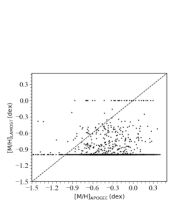
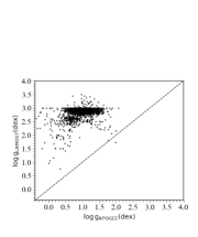
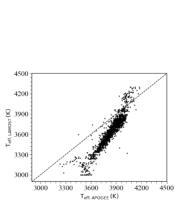
Figure 1: The comparison of metallicity, surface gravity and effective temperature between LAMOST and APOGEE of 2123 M giant stars, respectively.

2.2 Training set

In this work, we train the SLAM model to predict the stellar parameters of M giant stars. The training set is used to train the model of the stellar labels versus the spectra. This requires that the spectra of the training set should have high signal to noise ratios (SNRs) and the accurate labels to each spectrum, e. g. [M/H], [$\alpha$/M], ${T_{\mathrm{eff}}}$ and log$\,{\mathrm{g}}$ in this work. To this way, we cross-match the whole sample of M giant stars with APOGEE DR17 (Abdurro’uf et al. 2022) and obtain a common catalog of 4473 M giant stars. With following criteria, we further constrain the accuracy of the stellar parameters ${T_{\mathrm{eff}}}$, log $g$, [M/H] and [$\alpha$/M] , at last 3670 M giant stars are left for the training set, including the accurate stellar parameters from APOGEE DR17 and high SNR spectra from LAMOST DR9.

1. $\mathrm{SNR}>50$

2. $\sigma_{[\mathrm{M/H}]}<0.1$

3. $\sigma_{T_{\mathrm{eff}}}<20$

4. $\sigma_{\mathrm{log}\,g}<0.1$

5. $\sigma_{[\mathrm{\alpha/M}]}<0.05$

where SNR is the mean signal-to-noise ratio of LAMOST spectra as described in subsection 2.1, $\sigma_{[\mathrm{M/H}]}$, $\sigma_{T_{\mathrm{eff}}}$, $\sigma_{\mathrm{log}\,g}$ and $\sigma_{[\mathrm{\alpha/M}]}$ are the uncertainties of the metallicity [M/H], the effective temperature $T_{\mathrm{eff}}$, the surface gravity $\mathrm{log}\,g$ and the alpha abundance ${[\mathrm{\alpha/M}]}$ of the M giant stars, which are provided by APOGEE DR17.

The excluded 803 stars will be used in the subsection 3.2.4 to verify the self consistency of the trained model in deriving the stellar parameters. Figure 2 shows the Hertzsprung Russell diagram (HRD) of the 3670 common M giants stars, which are color-coded by the metallicity [M/H]. We find that all the training samples are located in the ranges of -1.5 $<$ [M/H] $<$ 0.5 dex, 3200 $<$ ${T_{\mathrm{eff}}}$ $<$ 4300 k, -0.4 $<$ log$\,g$ $<$ 2.5 dex. For comparison, we also represent the isochrones from the PAdova and TRieste Stellar Evolution Code (PARSEC; Bressan et al. 2012) with the dashed lines of the same age of 3 Gyr and different metallicities of 0.3, 0, -0.3 and -0.6 dex. As showed in the later results, this is reasonable for our sample, majority of which are the thin disk members. Statistically speaking, the distribution of the training stellar labels are consistent with the stellar evolution model and the M giant stars are mainly the metal rich stars.

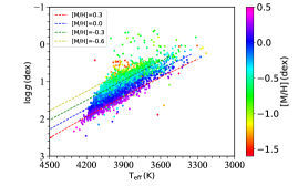
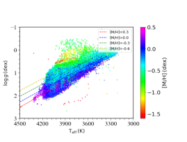
Figure 2: The distributions in the HR diagram of the training set and the prediction M giants with SNR $>$ 50 are showed color-coded by the metallicity [M/H] in the left and right panels, respectively. In the left panel, the stellar parameters of 3670 M giant stars are from APOGEE. In the right panel, the stellar parameters of the M giant sample with SNR $>$ 50 are predicted by SLAM. The dashed lines in both panels represent the isochrones from PARSEC model with the same age 3 Gyr but different metallicities, i.e. -0.6, -0.3, 0 and 0.3 dex for the yellow, green, blue and red lines, respectively.

3 Method and Results

3.1 Radial Velocity

The radial velocity is derived by using cross correlation based method laspec (Zhang et al. 2021). It is applied on the spectra of M giant stars with wavelength between 8000 to 8950 Å  from LAMOST DR9, where Ca II triplet is included in this band. The results can be evaluated by the following equation,

$${\rm CCF}(v|F,G)=\frac{{\rm Cov}(F,G(v))}{\sqrt{{\rm Var}(F){\rm Var}(G(v))}}$$ (1)

where $F$ is the normalized observed spectrum of the given M giant star, while $G$ is the synthetic spectra from ATLAS9 (Allende Prieto et al. 2018), also with wavelength between 8000 to 8950 Å  with a shift caused by the radial velocity. It is noteworthy that the spectra used in subsection 3.2 have been shifted back to the rest frame by the radial velocity.

To evaluate the results, we cross match our sample with Gaia DR3 (Gaia DR3; Katz et al. 2022; Gaia Collaboration 2022) and APOGEE DR17 (Abdurro’uf et al. 2022) to obtain two datasets of common stars. There are 32787 and 4888 common stars with Gaia DR3 and APOGEE DR17, respectively. Then the comparison of our results with Gaia DR3 and APOGEE DR17 are represented by the blue and red symbols in the Figure 3, respectively. It shows a good agreement between our results with that from Gaia DR3 and APOGEE DR17. The histogram of the radial velocity difference $\rm\Delta rv=rv-rv\rm_{Ref}$ are showed in the right panel. The system offset and scatter values of $\rm\Delta rv$ are around $\sim$ 1 km s^-1 and 4.6 km s^-1, respectively, for both comparison results. It indicates that the radial velocity of M giants derived form Ca II Triplet lines is consistent with that of Gaia DR3 and APOGEE DR17.

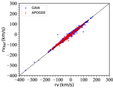
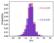
Figure 3: Compared the radial velocity from this work with that in Gaia DR3 (32787 stars) and APOGEE DR17 (4888 stars), as displayed by the red and blue colors in the left panel, respectively. The right panel displays the corresponding histograms of radial velocity difference $\rm\Delta rv$, where rv is the radial velocity derived in this work, and rv_Ref is the radial velocity from Gaia DR3 (blue) and APOGEE DR17 (red).

3.2 Stellar Parameter

The Stellar LAbel Machine (SLAM) is a data-driven method based on support vector regression (SVR) (Zhang et al. 2020). SVR is a robust nonlinear regression which has been applied in many fields of astronomy (Liu et al. 2012, 2015). SVR has been particularly widely used in spectral data analysis (Li et al. 2014; Liu et al. 2014; Bu & Pan 2015). This method has been proved to have good performance in determining stellar atmospheric parameters from spectra (Zhang et al. 2020; Li et al. 2021; Guo et al. 2021). In this work, we also adopt SLAM to derive the atmospheric parameters of the M giants.

3.2.1 Stellar label model training

In SLAM, the radial basis function (RBF) is adopted as the kernel of SVR. The hyperparameters $C$, $\varepsilon$ and $\gamma$ of SLAM represent the penalty level, tube radius and the width of the RBF kernel, respectively. These three hyperparameters can be automatically determined for each pixel through the training set.

$\boldsymbol{\vec{\theta}}_{i}$ is denoted as the stellar label vector of the $i$th star in the training set. f_j($\boldsymbol{\vec{\theta}}_{i}$) and $f_{i,j}$ are defined as the $j$th pixel of the training spectrum and model output spectrum corresponding to the the stars with stellar label vector $\boldsymbol{\vec{\theta}}_{i}$. The mean squared error (MSE) and median deviation (MD) of $j$th pixel can be evaluated with a specific set of hyperparameters, described by Equations (2) and (3)

$$MSE_{\emph{j}}=\frac{1}{m}\sum_{i=1}^{m}\big{[}\emph{f${}_{j}$}\big{(}\boldsymbol{\vec{\theta}}_{i}\big{)}-\emph{f${}_{i,j}$}\big{]}^{2}$$ (2)

$$MD_{\emph{j}}=\frac{1}{m}\sum_{i=1}^{m}\big{[}\emph{f${}_{j}$}\big{(}\boldsymbol{\vec{\theta}}_{i}\big{)}-\emph{f${}_{i,j}$}\big{]}$$ (3)

Theoretically, the smaller MSE and MD are, the better fitting is. However, we probably get an overfitted model if we train the SLAM model by whole training set, i.e., the $\rm MSE_{\emph{j}}$ and $\rm MD_{\emph{j}}$ are all equal to 0. Zhang et al. (2020) used the k-fold cross-validated MSE (CV MSE) and $k$-flod cross-validated MD (CV MD) to measure MSE_j and MD_j to avoid getting an overfitted trained model. Namely, the training set is randomly divided into $k$ subsets, where $k$ is set to be 10 in this work. The f_j($\boldsymbol{\vec{\theta}}_{i}$) is predicted by the model which trained by the other $k-1$ subsets of the training set. After looping through all the hyperparameters sets specified, the best set of hyperparameters can be determined for $j$th pixel by searching for the lowest CV MSE_j. The best model can be obtained for each pixel by doing pixel-to-pixel. In this work, we train SLAM model with 3670 low-resolution spectra from LAMOST of the training sample and their corresponding stellar labels from APOGEE.

3.2.2 Prediction of stellar labels

Using the Bayesian formula, the posterior probability density function of stellar label vector for a given observed spectrum is displayed in Equation (4).

$$p\big{(}\boldsymbol{\vec{\theta}}\mid\boldsymbol{\vec{f}}_{obs}\big{)}\propto p\big{(}\boldsymbol{\vec{\theta}}\big{)}\prod_{j=1}^{n}p\big{(}f_{j,obs}\mid\boldsymbol{\vec{\theta}}\big{)}$$ (4)

where $\boldsymbol{\vec{\theta}}$ is the stellar label vector, $\boldsymbol{\vec{f}}_{obs}$ and f_j,obs represent the normalized observed spectrum vector and the normalized flux of jth pixel of the observed spectrum, respectively. $p(\boldsymbol{\vec{\theta}})$ is the prior of stellar label vector $\boldsymbol{\vec{\theta}}$, $p(f_{j,obs}\mid\boldsymbol{\vec{\theta}})$ is the likelihood of observed spectrum flux of jth pixel with a given stellar label vetor $\boldsymbol{\vec{\theta}}$. By maximizing the posterior probability $p(\boldsymbol{\vec{\theta}}\mid\boldsymbol{\vec{f}}_{obs})$, the stellar labels can be easily measured with a Gaussian likelihood adopted. Then the logarithmic form of likelihood is described by the following equation,

$$\begin{split}\ln p\big{(}\boldsymbol{\vec{\theta}}\mid\boldsymbol{\vec{f}}_{obs}\big{)}=&-\frac{1}{2}\sum_{j=1}^{n}\times\frac{\big{[}f_{j,obs}-f_{j}\big{(}\boldsymbol{\vec{\theta}}\big{)}\big{]}^{2}}{\sigma_{j,obs}^{2}+\sigma_{j}\big{(}\boldsymbol{\vec{\theta}}\big{)}^{2}}\\ &-\frac{1}{2}\sum_{j=1}^{n}\times\ln\big{[}2\pi\big{(}\sigma_{j,obs}^{2}+\sigma_{j}\big{(}\boldsymbol{\vec{\theta}}\big{)}^{2}\big{)}\big{]}\end{split}$$ (5)

where $f_{j}\big{(}\boldsymbol{\vec{\theta}}\big{)}$ and $\sigma_{j}(\boldsymbol{\vec{\theta}})$ are the model output spectrum and the uncertainty of jth pixel corresponding to stellar label $\boldsymbol{\vec{\theta}}$, respectively. $f_{j,obs}$ is the $j$th pixel of the normalized observed spectrum, and $\sigma_{j,obs}$ is the uncertainty of jth pixel of normalized observed spectrum.

The trained model as described in subsection 3.2.1 is applied on the spectra of all the M giant stars to obtain their atmospheric parameters. The right panel of Figure 2 illustrates the distribution of the effective temperature $T_{\mathrm{eff}}$ versus surface gravity $\mathrm{log}\,g$ of the prediction M giant stars with SNR $>$ 50, accounting for 80% of the whole M giant stars. The color is coded by the metallicity [M/H]. It exhibits a similar pattern with that of the training sample as showed in the left panel of Figure 2. The same isochrones are also represented by the dashed lines with those in the first panel of Figure 2.

3.2.3 Stellar label uncertainty

Similar to the CV MSE and CV MD of spectrum as described in 3.2.1, Equations (6) and (7) describe the cross-validate scatter (CV_scatter) and cross-validate bias (CV_bias) of stellar labels, respectively. Obviously, if the predicted stars have the known stellar label, the CV_scatter and CV_bias can be measured. They can be regarded as the standard deviation and average deviation of the stellar labels, respectively, to describe the precision of the stellar parameters determined from SLAM model. In principle, the smaller CV_bias and CV_scatter indicate a better trained model.

$$CV\_bias=\frac{1}{m}\sum_{i=1}^{m}\big{(}\boldsymbol{\vec{\theta}}_{i,SLAM}-\boldsymbol{\vec{\theta}}_{i}\big{)}$$ (6)

$$CV\_scatter=\frac{1}{m}\sqrt{\sum_{i=1}^{m}\big{(}\boldsymbol{\vec{\theta}}_{i,SLAM}-\boldsymbol{\vec{\theta}}_{i}\big{)}^{2}}$$ (7)

where $\boldsymbol{\vec{\theta}}_{i,SLAM}$ is the stellar label vector from the model prediction, and $\boldsymbol{\vec{\theta}_{i}}$ is the corresponding true stellar label vector.

Figure 4 shows the distributions of CV bias (blue) and scatter (red) of the four parameters versus the SNR of spectra, i.e. the metallicity [M/H], the effective temperature $T_{\mathrm{eff}}$, the surface gravity $\mathrm{log}\,g$ and the alpha abundance [$\alpha$/M]. It is obvious that the CV scatters of these four parameters decrease with increasing SNR, e.g. from 0.27 dex, 110 K, 0.39 dex, 0.12 dex at SNR=17 to 0.16 dex, 57 K, 0.25 dex and 0.06 dex at SNR=100 for [M/H], $T_{\mathrm{eff}}$, log$\,g$ and [$\alpha$/M], respectively. In other words, the precision of these four parameters determined form SLAM model can reach to 0.16 dex, 57 K, 0.25 dex and 0.06 dex at SNR $>$ 100, respectively. The mean values of CV bias are -0.01 dex, -5 K, 0.02 dex and -0.01 dex for these four parameters, respectively, which means that the predicted parameters by SLAM are in good agreement with the true stellar labels given by APOGEE.

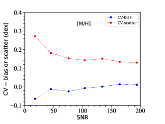
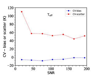
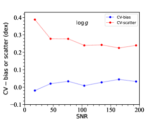
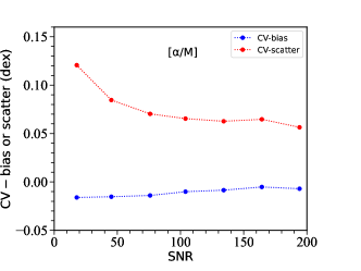
Figure 4: Four panels exhibit the CV scatter and bias as a function of SNR for [M/H], $T_{\mathrm{eff}}$, log$\,g$ and [$\alpha$/M], respectively. The red and blue dotted lines indicate the CV scatter and CV bias in different SNR bins, respectively.

3.2.4 Stellar labels self-consistent

In order to verify the self consistency of stellar labels determined from SLAM model. The training set is randomly split into two subsets, a training set consists of 2770 M giants, the remaining 900 M giants are used as the test set. Besides, the 803 M giant stars mentioned in subsection 2.2 are also used as the test set. Figure 5 displayed the comparison of four stellar labels between the true values and the model prediction values. In the left four panels, the black and red dots display the $\rm X_{AP}$ vs. $\rm X_{SLAM}$ of 900 stars with SNR$>50$ and 803 stars with SNR$<50$ in the test set, respectively, where X can be [M/H], $T_{\mathrm{eff}}$, log$\,g$ and [$\alpha$/M], respectively. It is obviously that the model prediction stellar labels are agreement with the true stellar labels. However, the distribution between $\rm X_{AP}$ and $\rm X_{SLAM}$ of stars with low SNR (red dots) is more dispersed than that of stars with high SNR (black dots). As shown in the four right panels, the red and black histograms exhibit the distribution of $\rm\Delta X$ = $\rm X_{AP}$-$\rm X_{SLAM}$ of stars with SNR $>$ 50 and stars with SNR $<$ 50. The mean values of $\rm\Delta X$ of two subsamples are close to 0, but the scatter values of stars with low SNR is larger than that of stars with higher SNR. Because the spectra with low signal-to-noise ratio are more difficult to obtain high-precision stellar parameters.

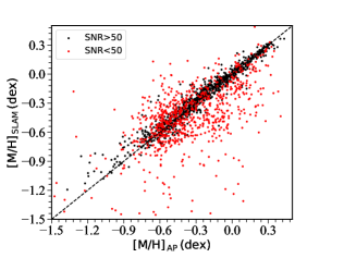
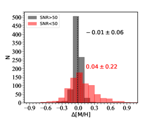
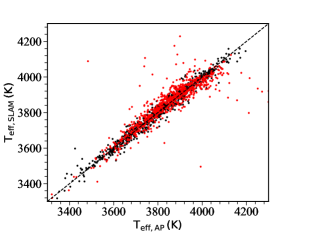
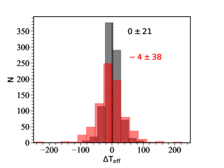
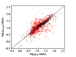
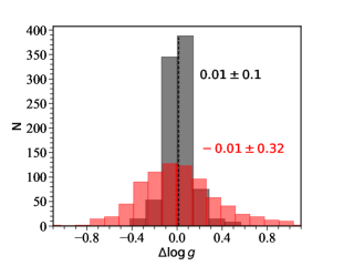
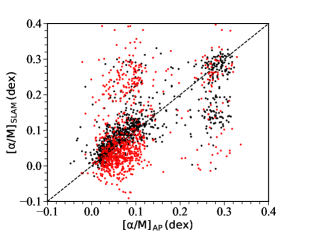
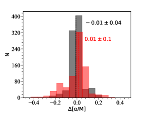
Figure 5: Four panels on the left display the comparison of stellar labels between the true values $\rm X_{AP}$ and model prediction values $\rm X_{SLAM}$, where X can be [M/H], $T_{\mathrm{eff}}$, log$\,g$ and [$\alpha$/M]. The black and red dots represent the stars with SNR$>50$ and SNR$<50$, respectively. The black dashed line is the one to one line in these four panels. The histograms of $\rm\Delta X$ (= $\rm X_{AP}$-$\rm X_{SLAM}$) as exhibited in the right four panels. The black and red histograms show the $\rm\Delta X$ of stars with SNR $>$ 50 and stars with SNR $<$ 50, respectively. The mean values of $\rm\Delta X$ of two subsamples as marked by the black and red dashed lines.

3.2.5 Stellar labels validation

We take a comparison of four stellar parameters with Li et al. (2022). They designed a deep convolution neural network with training stellar labels from APOGEE DR17 to derived the $T_{\mathrm{eff}}$, log $g$ and other 12 chemical abundance of 1,210,145 LAMOST DR8 giants with low resolution spectra (R $\sim$1800). 11,132 common stars were obtained in our samples and Li et al. (2022). The comparison of [M/H], $T_{\mathrm{eff}}$, log $g$ and [$\alpha$/M] are displayed in the left four panels in Figure 6. It obviously shows that the parameters in this work are consistent with that in Li et al. (2022). The corresponding histograms of $\rm\Delta X$= X_SLAM-X_Li are illustrated in the right four panels of Figure 6. The systematic offset between $T_{\mathrm{eff,SLAM}}$ and $T_{\mathrm{eff,Li}}$ is 7 K with a scatter of 32 K. For [M/H], log $g$ and [$\alpha$/M], there are very small biases (0.01 0.03 dex) between this work and Li et al. (2022) with scatters of 0.16 dex, 0.31 dex and 0.05 dex, respectively. It demonstrates that these four parameters in this work are consistent with that of Li et al. (2022).

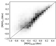
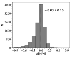
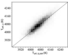
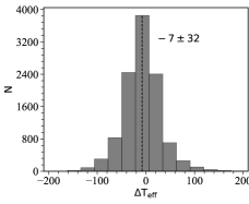
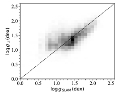
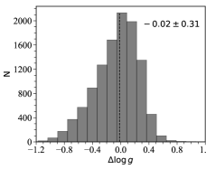
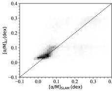
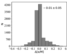
Figure 6: The comparison of [M/H], $T_{\mathrm{eff}}$, log $g$ and [$\alpha$/M] of 11,132 common stars in this work and Li et al. (2022). The left four panels from top to the bottom display the distributions of X_SLAM and X_Li, where X can be [M/H], T$\rm{eff}$, log $g$ and [$\alpha$/M], respectively. The subscript ’SLAM’ illustrates the parameters from this work and subscript ’Li’ represents that from Li et al. (2022). The black dotted lines in the left four panels are the one-to-one line. The corresponding histograms of the parameter difference $\rm\Delta X$= X_SLAM-X_Li as shown in the right four panels. The mean value of $\rm\Delta X$ as marked by the black dotted lines in the right panels.

3.3 Distance

In the selected M giant stars, most of them are the red giant branch stars and a few asymptotic giant branch stars. In order to calculate the distance, we firstly constrain the absolute magnitude for each M giant star. Here we assume the absolute magnitude $K_{\mathrm{abs}}$ is a function $D$ of the intrinsic color index $c_{0}$ and metallicity $M$, i.e. $K_{\mathrm{abs}}=D(c_{0},M)$. As showed by Majewski et al. (2003), Li et al. (2016a) and Figure 2, the M giant stars are mainly tracing the metal rich components, such as the disk or the Sagittarius Stream, the $J$ and $K-$band magnitudes are adopted to determine the distance to reduce the extinction effect from dust.

Assuming the $i$th star has the apparent magnitudes $J_{i}$ and $K_{i}$ and the distance $d_{i}$, and suffers the extinction $A^{K}_{i}(d_{i})$, where $A^{K}(d_{i})$ is a function of distance $d_{i}$, then we have the following relation where both sides are the absolute magnitude $K_{\mathrm{abs}}$,

$$K_{i}-A^{K}_{i}(d_{i})-5\times\mathrm{log}\,(100\times d_{i})=D(c_{0},M)$$ (8)

where $c_{0}$ is the intrinsic color index, which can be calculated by

$$c_{0}=(J-K)-(A^{J}(d)-A^{K}(d))$$ (9)

Then we can find that only the true distance $d$ satisfies the Equations (8) and (9). Here the 3D dust map from Green et al. (2019) is adopted, which has a median uncertainty around $30\%$.

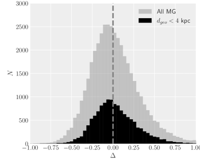
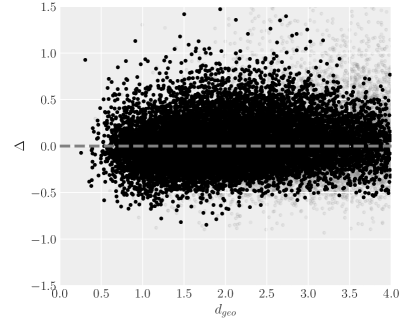
Figure 7: The distance comparison with $r_{\mathrm{geo}}$ from (Bailer-Jones et al. 2021) is showed. The histogram distribution of the relative difference $\Delta=(d_{\mathrm{MCM}}-d_{\mathrm{geo}})/d_{\mathrm{geo}}$is showed the left panel. The distribution of relative difference versus the distance is showed in the right panel. In both panel, the gray symbols represent the distribution of all the samples with predicted metallicity between -0.9 and 0.5. While the black ones represent the samples with distance $d_{\mathrm{geo}}<4$ kpc and its signal to noise ratio larger than 20.

Following Tian et al. (2020), we show the distributions of the comparison of the predicted distance $d_{\mathrm{MCM}}$ with that obtained from parallax (Bailer-Jones et al. 2021), $d_{\mathrm{geo}}$. The subsample with reliable distances are selected with $d_{\mathrm{geo}}<4$ kpc and the $d_{\mathrm{geo}}/\sigma_{d_{\mathrm{geo}}}>20$. Meanwhile the metallicity is also limited to be between -0.9 and 0.5. Then the distributions of the relative distance difference $\Delta=(d_{\mathrm{MCM}}-d_{\mathrm{geo}})/d_{\mathrm{geo}}$ of the subsample are showed in the Figure 7. The comparison shows a median difference $0.2\%$ and the 16% and 84% percentage values of 21.2% and 27.5%., which indicate a very small system offset and statistical dispersion smaller than 30%. In the right panel, the relative distance difference is represented versus the distance $d_{\mathrm{geo}}$. There is not significant relation between the system offset versus the distance.

4 Discussion

With the distances and radial velocity combining the astrometric information from Gaia, we are able to calculate the full 6D information, positions $(X,Y,Z)$ and velocities $(U,V,W)$. Figure 8 shows the space distributions of the M giant stars. The location of the Sun is represented by the dashed lines. We can find that most of the M giant stars are located in the disk, $|Z|<5$ kpc, meanwhile, there are also few M giant stars of larger heights, which are possible the member stars of the Sagittarius Stream.

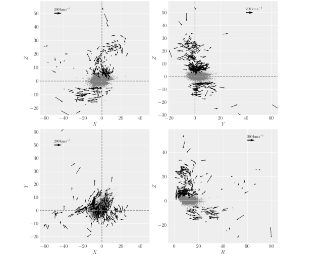
Figure 8: The space distributions are showed in different spaces. The velocities of the samples with larger height $|Z|>5$ kpc in the corresponding space are represented by the arrows. The Sun is located at $(X,Y,Z)=(0,0,0)$ kpc and $(R,Z)=(8.34,0)$ kpc.

4.1 Disks

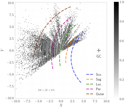
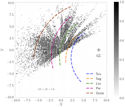
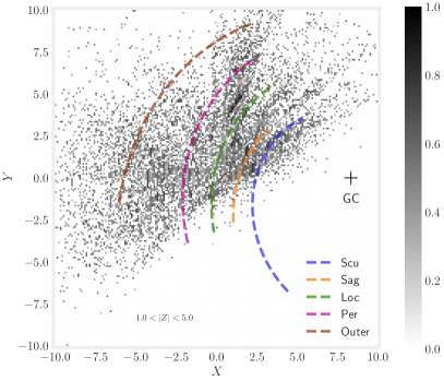
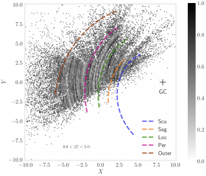
Figure 9: Disk rotational velocity distribution after line integral convolution with different heights.

As showed in Figure 8, majority of our sample are the disk stars, which are located with height smaller than $5$ kpc. Figure 9 shows the movements of disk traced by the M giant stars with different heights. The five known spiral arms are represented by the dashed curves from Chen et al. (2019). The distributions of the line integral convolution show clear streaming movement which are the rotation of the disk, especially the thin disk represented by the subsample with $|Z|<0.5$ kpc.

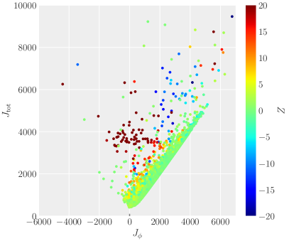
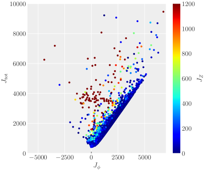
Figure 10: The distribution of the M giant stars in the action space $J_{\phi}$ versus $J_{\mathrm{tot}}$ are showed, which are color-coded by the height $Z$ and action $J_{Z}$ in the left and right panels, respectively.

Figure 10 shows the phase space distribution of the M giant stars, $J_{\phi}$ versus $J_{\mathrm{tot}}$. The samples are color-coded by the height $Z$ to the disk plane and the action $J_{Z}$ in the left and right panels, respectively. The action distributions also prove that the majority of the M giant stars are concentrated in the thin cyan and blue belt in the left and right panels, respectively, which are the disk with low height $|Z|$ and action $J_{Z}$.

4.2 Sagittarius Stream

Another application for the M giant sample is to trace the Sagittarius Stream (Majewski et al. 2003; Li et al. 2016a). From the Figures 8 and 10, there are also a few stars with larger heights $|Z|>5$ kpc, whose movements are also represented by the arrows. From previous studies (Majewski et al. 2003; Li et al. 2016a), the Sagittarius Stream has a significant contribution to the M giant stars with high latitude. In Figure 8, those M giant stars with larger heights show significant bulk motions, especially those stars with $Z$ around $25$ kpc and $-10$ kpc. That is more clear in Figure 10, where those samples are of larger total actions $J_{\mathrm{tot}}$ and small angular momentum $J_{\phi}$, which are completely different with those belong to the disk. To further illustration, we convert the coordinate $(\alpha,\delta)$ to that based on the Sagittarius Stream plane $(\Lambda,B)$, where the north pole $B=90^{\circ}$ is set to the same direction of the normal of the orbit plane of the Sagittarius Stream. Then Figure 11 shows the distance variance versus the longitude $\Lambda$ color-coded by the latitude $|B|$. The mock data for the Sagittarius Stream from Law & Majewski (2010) is also showed with gray dots. We find that the distance distribution of those M giant stars fits the model well. There are also few nearby stars offset the model which are possible the flared disk stars with $|Z|>5$ kpc. That can be proved by the action distributions as showed in Figure 10.

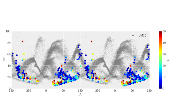
Figure 11: The distance distribution versus longitude $\Lambda$ of the M giant stars with height larger than $5$ kpc is showed which are color coded by the latitude $B$. The samples of the simulated Sagittarius Stream from LM10 are showed with gray symbols.

5 Summary

With similar method with Zhong et al. (2015), Zhong et al. (2019), Li et al (in preparation) select M giant stars from LAMOST DR9 with a very high purity. Many of those low temperature M giant stars are not given the stellar parameters and the radial velocities in the official catalog. In this work, we revise the spectra of those M giant stars and constrain the stellar parameter $(T_{\mathrm{eff}}$,$\mathrm{log}\,g$, $\mathrm{[M/H]})$, the chemical abundance $\mathrm{[\alpha/M]}$ and the radial velocities with uncertainties of $(57\,\mathrm{K},0.25\,\mathrm{dex},0.16\,\mathrm{dex},0.06\,\mathrm{dex})$ and $4.6$ km s^-1, respectively. With those information, we are able to calculate the full 6D information of M giants, and further to study the Milky Way disks and the Sagittarius Stream. Combining the geometric and phase space distributions, the disk and the Sagittarius Stream can be well separated. This value added sample will provide a pure sample for the chemical and kinematic studies for the disk and the Sagittarius Stream.

6 acknowledge

H.T. is supported by Beijing Natural Science Foundation with grant No. 1214028 and the National Natural Science Foundation of China (NSFC) under grants 12103062. J.L. would like to acknowledge the NSFC under grant 12273027 and China West Normal University grants 17YC507. C.L. thanks the National Natural Science Foundation of China (NSFC) with grant Nos.11835057 and the National Key R&D Program of China No. 2019YFA0405501. J.R.S. is supported by the National Key R&D Program of China No. 2019YFA0405502 and the National Natural Science Foundation of China under grant Nos. 12090040, 12090044, 11833006. M.Y. gratefully acknowledges support from the National Natural Science Foundation of China (Grant No.12133002). Guoshoujing Telescope (the Large Sky Area Multi-Object Fiber Spectroscopic Telescope LAMOST) is a National Major Scientific Project built by the Chinese Academy of Sciences. Funding for the project has been provided by the National Development and Reform Commission. LAMOST is operated and managed by the National Astronomical Observatories, Chinese Academy of Sciences.

Appendix A Catalog sample

Table 1 lists the information in our catalog, including the observational ID, (obsid), the mean signal to noise ratio (SNR) of LAMOST spectra and the coordinates (ra_obs, dec_obs) from LAMOST. The stellar parameters, the distance, the radial velocities and their uncertainties are also provided. The whole catalog is available to download through the link https://nadc.china-vo.org/res/r101196/.

Table 1: Catalog description of $\sim$ 43,000 M giants

Column	units	Description
obsid		LAMOST observe id
ra_obs	deg	right ascension from LAMOST
dec_obs	deg	declination from LAMOST
SNR		mean signal to noise ratio of LAMOST spectra
[M/H]	dex	[M/H] from SLAM
[M/H]err	dex	[M/H] uncertainty
$T_{\mathrm{eff}}$	K	Teff from SLAM
${T_{\mathrm{eff}}}\rm_{err}$	K	$T_{\mathrm{eff}}$ uncertainty
$\mathrm{log}\,g$	dex	$\mathrm{log}\,g$ from SLAM
$\mathrm{log}\,g\rm_{err}$	dex	$\mathrm{log}\,g$ uncertainty
$\mathrm{[\alpha/M]}$	dex	$\mathrm{[\alpha/M]}$ from SLAM
$\mathrm{[\alpha/M]}\rm_{err}$	dex	$\mathrm{[\alpha/M]}$ uncertainty
rv	$\rm km\,s^{-1}$	radial velocity
Distance	kpc	Distance of M giants

References

- Abdurro’uf et al. (2022) Abdurro’uf, Accetta, K., Aerts, C., et al. 2022, ApJS, 259, 35, doi: 10.3847/1538-4365/ac4414
- Ahumada et al. (2020) Ahumada, R., Prieto, C. A., Almeida, A., et al. 2020, ApJS, 249, 3, doi: 10.3847/1538-4365/ab929e
- Allende Prieto et al. (2018) Allende Prieto, C., Koesterke, L., Hubeny, I., et al. 2018, A&A, 618, A25, doi: 10.1051/0004-6361/201732484
- Antoniadis-Karnavas et al. (2020) Antoniadis-Karnavas, A., Sousa, S. G., Delgado-Mena, E., et al. 2020, A&A, 636, A9, doi: 10.1051/0004-6361/201937194
- Bailer-Jones et al. (2021) Bailer-Jones, C. A. L., Rybizki, J., Fouesneau, M., Demleitner, M., & Andrae, R. 2021, AJ, 161, 147, doi: 10.3847/1538-3881/abd806
- Belokurov et al. (2014) Belokurov, V., Koposov, S. E., Evans, N. W., et al. 2014, MNRAS, 437, 116, doi: 10.1093/mnras/stt1862
- Bizyaev et al. (2010) Bizyaev, D., Smith, V. V., & Cunha, K. 2010, AJ, 140, 1911, doi: 10.1088/0004-6256/140/6/1911
- Bizyaev et al. (2006) Bizyaev, D., Smith, V. V., Arenas, J., et al. 2006, AJ, 131, 1784, doi: 10.1086/500243
- Bressan et al. (2012) Bressan, A., Marigo, P., Girardi, L., et al. 2012, MNRAS, 427, 127, doi: 10.1111/j.1365-2966.2012.21948.x
- Bu & Pan (2015) Bu, Y., & Pan, J. 2015, MNRAS, 447, 256, doi: 10.1093/mnras/stu2063
- Carlin et al. (2018) Carlin, J. L., Sheffield, A. A., Cunha, K., & Smith, V. V. 2018, ApJ, 859, L10, doi: 10.3847/2041-8213/aac3d8
- Castelli & Kurucz (2003) Castelli, F., & Kurucz, R. L. 2003, in Modelling of Stellar Atmospheres, ed. N. Piskunov, W. W. Weiss, & D. F. Gray, Vol. 210, A20. https://arxiv.org/abs/astro-ph/0405087
- Chen et al. (2019) Chen, B. Q., Huang, Y., Hou, L. G., et al. 2019, MNRAS, 487, 1400, doi: 10.1093/mnras/stz1357
- Chene et al. (2014) Chene, A.-N., Padzer, J., Barrick, G., et al. 2014, in Society of Photo-Optical Instrumentation Engineers (SPIE) Conference Series, Vol. 9151, Advances in Optical and Mechanical Technologies for Telescopes and Instrumentation, ed. R. Navarro, C. R. Cunningham, & A. A. Barto, 915147, doi: 10.1117/12.2057417
- Cui et al. (2012) Cui, X.-Q., Zhao, Y.-H., Chu, Y.-Q., et al. 2012, Research in Astronomy and Astrophysics, 12, 1197, doi: 10.1088/1674-4527/12/9/003
- Deng et al. (2012) Deng, L.-C., Newberg, H. J., Liu, C., et al. 2012, Research in Astronomy and Astrophysics, 12, 735, doi: 10.1088/1674-4527/12/7/003
- Ding et al. (2022) Ding, M.-Y., Shi, J.-R., Wu, Y., et al. 2022, ApJS, 260, 45, doi: 10.3847/1538-4365/ac6754
- Dotter et al. (2008) Dotter, A., Chaboyer, B., Jevremović, D., et al. 2008, ApJS, 178, 89, doi: 10.1086/589654
- Gaia Collaboration (2022) Gaia Collaboration. 2022, VizieR Online Data Catalog, I/355
- Galgano et al. (2020) Galgano, B., Stassun, K., & Rojas-Ayala, B. 2020, AJ, 159, 193, doi: 10.3847/1538-3881/ab7f37
- Green et al. (2019) Green, G. M., Schlafly, E., Zucker, C., Speagle, J. S., & Finkbeiner, D. 2019, ApJ, 887, 93, doi: 10.3847/1538-4357/ab5362
- Guo et al. (2021) Guo , Y., Zhang, B., Liu, C., et al. 2021, ApJS, 257, 54, doi: 10.3847/1538-4365/ac2ded
- Howard (2017) Howard, E. M. 2017, in Astronomical Society of the Pacific Conference Series, Vol. 512, Astronomical Data Analysis Software and Systems XXV, ed. N. P. F. Lorente, K. Shortridge, & R. Wayth, 245
- Ibata et al. (1994) Ibata, R. A., Gilmore, G., & Irwin, M. J. 1994, Nature, 370, 194, doi: 10.1038/370194a0
- Katz et al. (2022) Katz, D., Sartoretti, P., Guerrier, A., et al. 2022, arXiv e-prints, arXiv:2206.05902. https://arxiv.org/abs/2206.05902
- Koleva et al. (2009) Koleva, M., Prugniel, P., Bouchard, A., & Wu, Y. 2009, A&A, 501, 1269, doi: 10.1051/0004-6361/200811467
- Koposov et al. (2015) Koposov, S. E., Belokurov, V., Zucker, D. B., et al. 2015, MNRAS, 446, 3110, doi: 10.1093/mnras/stu2263
- Kurucz (1993) Kurucz, R. 1993, ATLAS9 Stellar Atmosphere Programs and 2 km/s grid. Kurucz CD-ROM No. 13. Cambridge, 13
- Law & Majewski (2010) Law, D. R., & Majewski, S. R. 2010, ApJ, 714, 229, doi: 10.1088/0004-637X/714/1/229
- Li et al. (2021) Li, J., Liu, C., Zhang, B., et al. 2021, ApJS, 253, 45, doi: 10.3847/1538-4365/abe1c1
- Li et al. (2016a) Li, J., Smith, M. C., Zhong, J., et al. 2016a, ApJ, 823, 59, doi: 10.3847/0004-637X/823/1/59
- Li et al. (2016b) Li, J., Liu, C., Carlin, J. L., et al. 2016b, Research in Astronomy and Astrophysics, 16, 125, doi: 10.1088/1674-4527/16/8/125
- Li et al. (2019) Li, J., FELLOW, L., Liu, C., et al. 2019, ApJ, 874, 138, doi: 10.3847/1538-4357/ab09ef
- Li et al. (2014) Li, X., Wu, Q. M. J., Luo, A., et al. 2014, ApJ, 790, 105, doi: 10.1088/0004-637X/790/2/105
- Li et al. (2022) Li, Z., Zhao, G., Chen, Y., Liang, X., & Zhao, J. 2022, MNRAS, doi: 10.1093/mnras/stac1959
- Liu et al. (2012) Liu, C., Bailer-Jones, C. A. L., Sordo, R., et al. 2012, MNRAS, 426, 2463, doi: 10.1111/j.1365-2966.2012.21797.x
- Liu et al. (2015) Liu, C., Fang, M., Wu, Y., et al. 2015, ApJ, 807, 4, doi: 10.1088/0004-637X/807/1/4
- Liu et al. (2017) Liu, C., Xu, Y., Wan, J.-C., et al. 2017, Research in Astronomy and Astrophysics, 17, 096, doi: 10.1088/1674-4527/17/9/96
- Liu et al. (2020) Liu, C., Fu, J., Shi, J., et al. 2020, arXiv e-prints, arXiv:2005.07210. https://arxiv.org/abs/2005.07210
- Liu et al. (2014) Liu, C.-X., Zhang, P.-A., & Lu, Y. 2014, Research in Astronomy and Astrophysics, 14, 423, doi: 10.1088/1674-4527/14/4/005
- Luo et al. (2012) Luo, A. L., Zhang, H.-T., Zhao, Y.-H., et al. 2012, Research in Astronomy and Astrophysics, 12, 1243, doi: 10.1088/1674-4527/12/9/004
- Luo et al. (2015) Luo, A. L., Zhao, Y.-H., Zhao, G., et al. 2015, Research in Astronomy and Astrophysics, 15, 1095, doi: 10.1088/1674-4527/15/8/002
- Majewski et al. (2003) Majewski, S. R., Skrutskie, M. F., Weinberg, M. D., & Ostheimer, J. C. 2003, ApJ, 599, 1082, doi: 10.1086/379504
- Newberg et al. (2002) Newberg, H. J., Yanny, B., Rockosi, C., et al. 2002, ApJ, 569, 245, doi: 10.1086/338983
- Su & Cui (2004) Su, D.-Q., & Cui, X.-Q. 2004, Chinese J. Astron. Astrophys., 4, 1, doi: 10.1088/1009-9271/4/1/1
- Tian et al. (2020) Tian, H., Liu, C., Wang, Y., et al. 2020, ApJ, 899, 110, doi: 10.3847/1538-4357/aba1ec
- Tian et al. (2019) Tian, H., Liu, C., Xu, Y., & Xue, X. 2019, ApJ, 871, 184, doi: 10.3847/1538-4357/aaf6e8
- Tollestrup et al. (2012) Tollestrup, E. V., Pazder, J., Barrick, G., et al. 2012, in Society of Photo-Optical Instrumentation Engineers (SPIE) Conference Series, Vol. 8446, Ground-based and Airborne Instrumentation for Astronomy IV, ed. I. S. McLean, S. K. Ramsay, & H. Takami, 84462A, doi: 10.1117/12.926626
- Wang et al. (2020) Wang, R., Luo, A. L., Chen, J.-J., et al. 2020, ApJ, 891, 23, doi: 10.3847/1538-4357/ab6dea
- Wang et al. (1996) Wang, S.-G., Su, D.-Q., Chu, Y.-Q., Cui, X., & Wang, Y.-N. 1996, Appl. Opt., 35, 5155, doi: 10.1364/AO.35.005155
- Wu et al. (2014) Wu, Y., Du, B., Luo, A., Zhao, Y., & Yuan, H. 2014, in Statistical Challenges in 21st Century Cosmology, ed. A. Heavens, J.-L. Starck, & A. Krone-Martins, Vol. 306, 340–342, doi: 10.1017/S1743921314010825
- Xu et al. (2018) Xu, Y., Liu, C., Xue, X.-X., et al. 2018, MNRAS, 473, 1244, doi: 10.1093/mnras/stx2361
- Xu et al. (2020) Xu, Y., Liu, C., Tian, H., et al. 2020, ApJ, 905, 6, doi: 10.3847/1538-4357/abc2cb
- Yan et al. (2022) Yan, H., Li, H., Wang, S., et al. 2022, The Innovation, 3, 100224, doi: 10.1016/j.xinn.2022.100224
- Zhang et al. (2020) Zhang, B., Liu, C., & Deng, L.-C. 2020, ApJS, 246, 9, doi: 10.3847/1538-4365/ab55ef
- Zhang et al. (2021) Zhang, B., Li, J., Yang, F., et al. 2021, ApJS, 256, 14, doi: 10.3847/1538-4365/ac0834
- Zhao et al. (2012) Zhao, G., Zhao, Y., Chu, Y., Jing, Y., & Deng, L. 2012, arXiv e-prints, arXiv:1206.3569. https://arxiv.org/abs/1206.3569
- Zhong et al. (2019) Zhong, J., Li, J., Carlin, J. L., et al. 2019, ApJS, 244, 8, doi: 10.3847/1538-4365/ab3859
- Zhong et al. (2015) Zhong, J., Lépine, S., Li, J., et al. 2015, Research in Astronomy and Astrophysics, 15, 1154, doi: 10.1088/1674-4527/15/8/005