Electron wave functions in beta-decay formulas revisited (II): Completion including recoil-order and induced currents

Abstract

We present complete formulas of the allowed and first-forbidden transitions of the nuclear beta decay taking into account the recoil-order and induced currents up to the next-to-leading order (NLO). The longitudinal part of the vector current is cleared away by the use of the conservation of the vector current for the multipole operators of the natural-parity transitions, which makes the effect of the meson exchange current for the vector current as small as possible. The formula is transparent enough to be applied to various beta-decay processes. As a numerical demonstration, we apply our formulas to the beta decay of a neutron-rich nucleus ¹⁶⁰Sn. We find that the NLO corrections amount to 10–20% of the total decay rate, whereas the induced currents alter the rate at most 5%.

1 Introduction

Nuclear beta decay has attracted renewed interest. The astrophysical rapid-neutron-capture process, the r-process nucleosynthesis, is believed to produce more than half of heavier elements than iron. The beta decay is a predominant process in the freeze-out phase Mumpower:2015ova , and thus plays a decisive role in forming the abundance pattern. The detection of gravitational waves from a binary neutron-star merger and associated electromagnetic waves from a kilonova/macronova has provided an evidence of the r-process site abb17a ; abb17b . In such an exotic environment, heavy neutron-rich nuclei even close to the dripline are involved in the r-process.

An interest in the nuclear beta decay with a precise description also lies in neutrino physics, such as the reactor neutrino anomaly mention2011 ; hayes2014 and the search for the beyond-standard-model (BSM) physics Glick_Magid_2022 . The long-standing issue of nuclear physics, the effective (weak) axial vector coupling constant ($g_{A}^{\rm eff}$), might be resolved in the electron spectrum of the higher-order-forbidden transitions kostensalo2017 .

In our previous paper horiuchi2021electron [referred to as paper (I)], formulas of the beta-decay rate in a convenient and practical form were proposed. The nuclear beta decay was formulated using the effective multipole operators Koshigiri:1979zd ; morita1960theory . The analytic forms of the electron wave function in the next-to-leading order (NLO) of the integral equation of the electron Dirac equation and the formulas of the effective nuclear multipole operators were presented. It was demonstrated that the NLO formula reproduces well the ‘exact’ decay rate of the allowed Gamow–Teller and first-forbidden spin-dipole transitions for heavy nuclei with large $Z$, where the frequently used formulasch66 corresponding to a leading order formula of the systematic expansion in terms of nuclear radius, the Coulomb potential, the energy and the mass of electronBehrens:1971rbq , possibly overestimates the decay rates.

The formula in paper (I) is expressed in terms of the nuclear current density that is general enough to incorporate any models of the nuclear current such as many-body nuclear current in addition to the one-body current, non-relativistic and relativistic description of nuclear current. However, the explicit formula in the impulse approximation is given only for the leading $\bm{\sigma}\tau$ operator of the axial vector current. It is certainly necessary and valuable to update the formula of paper (I) by including the velocity-dependent terms such as $A_{0}\sim\bm{\sigma}\cdot\bm{p}/M\tau$, $\bm{V}\sim\bm{p}/M\tau$ and the induced currents.

In this paper, we give the formulas of the nuclear multipole operators using the non-relativistic impulse approximation of the nuclear current. The velocity-dependent terms of the time component of the axial-vector current, the space component of the vector current and the induced terms, i.e., the weak-magnetism term and the induced pseudo-scalar term, are included. These nuclear currents play an important role in the first-forbidden transitions. For the $0^{-}$ transition, for example, the time component of the axial-vector current competes with the spin-dipole operator towner1986 . The induced pseudo-scalar term would play a minor role in the nuclear beta decay. However, we keep it because the formulas can be used for the neutrino reactions including muon and tau leptons, while the so-called second class currents, the G-parity irregular terms weinberg58 ; wilkinson1977second , are not included.

In neutrino reactions and beta decay in the plane-wave approximation of lepton wave functions, a longitudinal part of the vector current is eliminated using the conservation of current, and further the LO term of the transverse electric current can be written in terms of the Coulomb multipole operator walecka2012semileptonic ; Nakamura:2000vp ; hayes2018 . In the beta decay or muon capture, because of the complication due to the Coulomb effect, this is done in the leading order of the long-wave-length approximation. In the muon capture, this was discussed in connection with the extended Siegert’s theorem fujii-fujita-morita-64 . In this paper, we rewrite the formula of paper (I) using the Fourier–Bessel transformation and the current conservation, which makes the effect of the meson-exchange current for the vector current as small as possible for the allowed and first-forbidden transitions. This work provides complete formulas of the allowed and first-forbidden transitions of the nuclear beta decay up to NLO within the non-relativistic impulse approximation of the nuclear current.

In section 2, the multipole operators for the parity $P=(-1)^{J}$ and $(-1)^{J+1}$ are given. The longitudinal part of the vector current is rewritten in terms of the time component of the vector current with the help of the current conservation. In section 3, a formula of the multipole operators in the impulse approximation is given. As a numerical demonstration of the usefulness of our method, the formula is applied to the beta decay of ¹⁶⁰Sn in section 4 together with the formula written in terms of nuclear transition densities. The transition densities are obtained by a nuclear energy-density-functional method. A summary is given in section 5.

2 Multipole expansion of the effective Hamiltonian

The effective Hamiltonian for the beta ($\beta^{\mp}$) decay is given by

$$H_{\mathrm{eff}}=\frac{G_{F}V_{ud}}{\sqrt{2}}\int d\bm{x}\left[\overline{e}(\bm{x})\gamma^{\mu}(1-\gamma_{5})\nu_{e}(\bm{x})J_{\mu}(\bm{x})+{\rm H.c.}\right],$$ (1)

where $G_{F}=1.166\times 10^{-5}$ GeV^-2 is the Fermi coupling constant and $V_{ud}=0.9737$ is the up-down element of the Cabibbo–Kobayashi–Maskawa matrix. This Hamiltonian consists of the electron field $e$, the neutrino field $\nu$, and the hadronic current

$$J^{\mu}(\bm{x})={\cal V}^{\mu}(\bm{x})-{\cal A}^{\mu}(\bm{x}),$$ (2)

with the vector [${\cal V}^{\mu}=(V^{0},\bm{V})$] and axial-vector [${\cal A}^{\mu}=(A^{0},\bm{A})$] currents. Using the multipole operator $\Xi_{JL}(\kappa_{e},\kappa_{\nu})$ constructed from partial waves of electron and neutrino specified in terms of $\kappa_{e}$ and $\kappa_{\nu}$ horiuchi2021electron , one obtains the rate of the $\beta^{\mp}$ decay from the initial ($i$) to final ($f$) nuclear states, $i\to f+e^{\mp}+\overline{\nu}_{e}(\nu_{e})$, as

$$\Gamma=\frac{\left(G_{F}V_{ud}\right)^{2}}{\pi^{2}}\int_{m_{e}}^{E_{0}}dE_{e}\,p_{e}E_{e}\left(E_{0}-E_{e}\right)^{2}\sum_{J,\kappa_{e},\kappa_{\nu}}\frac{1}{2J_{i}+1}\left|\sum_{L}\braket{f}{\Xi_{JL}\left(\kappa_{e},\kappa_{\nu}\right)}{i}\right|^{2},$$ (3)

where $J_{i}$ is the angular momentum of the initial nuclear state and $E_{0}$ is the maximum energy of the electron. The nonzero integers $\kappa_{e}$ and $\kappa_{\nu}$ represent the lepton angular momentum for the electron and neutrino, respectively, with

$$j_{\kappa}=|\kappa|-1/2,\hskip 28.45274ptl_{\kappa}=\begin{cases}\kappa&(\kappa>0)\\ -\kappa-1&(\kappa<0)\end{cases}.$$ (4)

The bracket $\braket{f}{\Xi_{JL}}{i}$ denotes the reduced matrix element (RDME) sakurai1985modern of the multipole operator $\Xi_{JL}$, which will be detailed in the next subsection.

2.1 Multipole operator

As shown in Eq. (12) of Ref. horiuchi2021electron , the multipole operator $\Xi_{JL}$ is written down as

$$\Xi_{JLM}(\kappa_{e},\kappa_{\nu}) =S_{\kappa_{e}}\int d\bm{r}$$

$$\times\left\{\mp Y_{JM}(\hat{r})V_{0}(\bm{r})\delta_{L,J}\Phi_{0JJ}(\kappa_{e},\kappa_{\nu};r)\right.\pm i[Y_{L}(\hat{r})\otimes\bm{V}(\bm{r})]_{JM}\phi_{1LJ}(\kappa_{e},\kappa_{\nu};r)$$

$$+iY_{JM}(\hat{r})A_{0}(\bm{r})\delta_{L,J}\phi_{0JJ}(\kappa_{e},\kappa_{\nu};r)-\left.[Y_{L}(\hat{r})\otimes\bm{A}(\bm{r})]_{JM}\Phi_{1LJ}(\kappa_{e},\kappa_{\nu};r)\right\},$$ (5)

where the plus-minus signs correspond to the $\beta^{\mp}$ decay. Here, $S_{\kappa}=\textrm{sgn}(\kappa)$ is the sign of $\kappa$ and

$$\Phi_{KLJ}(\kappa_{e},\kappa_{\nu};r) =G_{\kappa_{e}}(r)g_{\kappa_{\nu}}(r)S_{KLJ}(\kappa_{e},\kappa_{\nu})+F_{\kappa_{e}}(r)f_{\kappa_{\nu}}(r)S_{KLJ}(-\kappa_{e},-\kappa_{\nu}),$$ (6)

$$\phi_{KLJ}(\kappa_{e},\kappa_{\nu};r) =G_{\kappa_{e}}(r)f_{\kappa_{\nu}}(r)S_{KLJ}(\kappa_{e},-\kappa_{\nu})-F_{\kappa_{e}}(r)g_{\kappa_{\nu}}(r)S_{KLJ}(-\kappa_{e},\kappa_{\nu})$$ (7)

with

$$S_{KLJ}\left(\kappa^{\prime},\kappa\right)= \sqrt{2\left(2j_{\kappa}+1\right)\left(2j_{\kappa^{\prime}}+1\right)\left(2l_{\kappa}+1\right)\left(2l_{\kappa^{\prime}}+1\right)(2K+1)}$$

$$\times\left(l_{\kappa},0,l_{\kappa^{\prime}},0|L,0\right)\begin{Bmatrix}l_{\kappa^{\prime}}&1/2&j_{\kappa^{\prime}}\\ l_{\kappa}&1/2&j_{\kappa}\\ L&K&J\end{Bmatrix}.$$ (8)

Here $(j_{1},m_{1},j_{2},m_{2}|J,M)$ is the Clebsch–Gordan coefficient and the curly brackets denote the 9-j symbol rose1957ang ; edmonds1996angular . The radial wave functions of the emitted electron or the positron, $G_{\kappa}(r)$ and $F_{\kappa}(r)$, are obtained by solving the radial Dirac equation with the Coulomb potential $V_{C}(r)$ as

$$\frac{dG_{\kappa}(r)}{dr}+\frac{1+\kappa}{r}G_{\kappa}(r)-\left(m_{e}+E_{e}-V_{C}(r)\right)F_{\kappa}(r)=0,$$ (9)

$$\frac{dF_{\kappa}(r)}{dr}+\frac{1-\kappa}{r}F_{\kappa}(r)-\left(m_{e}-E_{e}+V_{C}(r)\right)G_{\kappa}(r)=0.$$ (10)

On the other hand, the neutrino is treated as a plane wave with the momentum $p_{\nu}=E_{0}-E_{e}$, and its radial wave functions are given by $g_{\kappa}(r)=j_{l_{\kappa}}\left(p_{\nu}r\right)$ and $f_{\kappa}(r)=S_{\kappa}j_{l_{-\kappa}}\left(p_{\nu}r\right)$, where $j_{l}(x)$ is the $l$th-order spherical Bessel function.

For a case of the angular momentum $J$ with the parity $P=(-1)^{J+1}$ such as $J^{P}=0^{-}$, $1^{+}$, and $2^{-}$, the multipole operator is written as

$$\sum_{L}\Xi_{JLM}(\kappa_{e},\kappa_{\nu}) =S_{\kappa_{e}}\int d\bm{r}\Big{\{}\pm i[Y_{J}(\hat{r})\otimes\bm{V}(\bm{r})]_{JM}\phi_{1JJ}(\kappa_{e},\kappa_{\nu};r)$$

$$+iY_{JM}(\hat{r})A_{0}(\bm{r})\phi_{0JJ}(\kappa_{e},\kappa_{\nu};r)$$

$$-\sum_{L=J\pm 1}[Y_{L}(\hat{r})\otimes\bm{A}(\bm{r})]_{JM}\Phi_{1LJ}(\kappa_{e},\kappa_{\nu};r)\Big{\}}.$$ (11)

The spatial component of the vector current (1st term) is the ‘magnetic’ operator, while that of the axial-vector current (3rd term) is the ‘electric’ operator. The time component (2nd term) and the spatial component (3rd term) of the axial vector current contribute to the $0^{-}$ operator.

For a case of the angular momentum $J$ with parity $P=(-1)^{J}$ such as $J^{P}=0^{+}$, $1^{-}$, and $2^{+}$, the multipole operator is written as

$$\sum_{L}\Xi_{JLM}(\kappa_{e},\kappa_{\nu}) =S_{\kappa_{e}}\int d\bm{r}\Big{\{}\mp Y_{JM}(\hat{r})V_{0}(\bm{r})\Phi_{0JJ}(\kappa_{e},\kappa_{\nu};r)$$

$$\pm i\sum_{L=J\pm 1}[Y_{L}(\hat{r})\otimes\bm{V}(\bm{r})]_{JM}\phi_{1LJ}(\kappa_{e},\kappa_{\nu};r)$$

$$-[Y_{J}(\hat{r})\otimes\bm{A}(\bm{r})]_{JM}\Phi_{1JJ}(\kappa_{e},\kappa_{\nu};r)\Big{\}}.$$ (12)

In this case, the spatial component of the vector current (2nd term) is the ‘electric’ operator, while the spatial component of the axial-vector current (3rd term) is the ‘magnetic’ operator. For the $0^{+}$ operator, the time component (1st term) and the spatial component (2nd term) of the vector current contribute to the transition.

2.2 Longitudinal component of the vector current

The meson-exchange current (MEC) for the spatial component of the isovector vector current plays an important role, while the impulse approximation works well for the time component of the vector current in most cases. Since it is rather hard to construct many-body nuclear currents that satisfy the current conservation relation consistent with the nuclear wave function obtained from the effective nuclear potential, it is effective to rewrite a part of the spatial component of the vector current in terms of the time component of the vector current and use the impulse approximation. Here we focus on the second term of Eq. (12) for the ‘electric’ transition. The first term of Eq. (11) has nothing to do with the current conservation law.

For the nuclear beta decay, due to the Coulomb distortion of the electron wave function, it is not straightforward to implement the current conservation relation in contrast to the plane-wave formula for neutrino reaction and beta decay rate walecka2012semileptonic ; Nakamura:2000vp . Here we use the Bessel–Fourier transformation to take advantage of the momentum space representation. The relevant terms of the multipole operator are written as

$$\sum_{L=J\pm 1}[Y_{L}(\hat{r})\otimes\bm{V}(\bm{r})]_{JM}\phi_{1LJ}(\kappa_{e},\kappa_{\nu};r) =\frac{2}{\pi}\int_{0}^{\infty}dq\,q^{2}\ {\cal O}^{J}(\kappa_{e},\kappa_{\nu};q),$$ (13)

where

$${\cal O}^{J}(\kappa_{e},\kappa_{\nu};q) =T^{JJ-1M}(q)\tilde{\phi}_{1J-1J}(\kappa_{e},\kappa_{\nu};q)+T^{JJ+1M}(q)\tilde{\phi}_{1J+1J}(\kappa_{e},\kappa_{\nu};q).$$ (14)

Here we used the identity,

$$\frac{2}{\pi}\int_{0}^{\infty}dqq^{2}j_{L}(qr)j_{L}(qr^{\prime}) = \frac{\delta(r-r^{\prime})}{r^{2}}.$$ (15)

The momentum-space multipole operator and lepton wave function are respectively defined as

$$T^{JLM}(q) =\int d\bm{r}\,j_{L}(qr)[Y_{L}(\hat{r})\otimes\bm{V}(\bm{r})]_{JM},$$ (16)

$$\tilde{\phi}_{1LJ}(\kappa_{e},\kappa_{\nu};q) =\int_{0}^{\infty}dr\,r^{2}j_{L}(qr)\phi_{1LJ}(\kappa_{e},\kappa_{\nu};r).$$ (17)

Hereafter, $\tilde{\phi}_{1LJ}(\kappa_{e},\kappa_{\nu};q)$ is simplified as $\tilde{\phi}_{L}(q)$.

The electric $T_{E}^{JM}$ and longitudinal $T_{L}^{JM}$ multipole operators are defined by

$$T_{E}^{JM}(q) =\frac{1}{q}\int d\bm{r}\,\bm{\nabla}\times[j_{J}(qr)\bm{Y}_{JJM}(\hat{r})]\cdot\bm{V}(\bm{r})$$

$$=-i\sqrt{\frac{J}{2J+1}}T^{JJ+1M}(q)+i\sqrt{\frac{J+1}{2J+1}}T^{JJ-1M}(q),$$ (18)

$$T_{L}^{JM}(q) =\frac{i}{q}\int d\bm{r}\,\bm{\nabla}[j_{J}(qr)Y_{JM}(\hat{r})]\cdot\bm{V}(\bm{r})$$

$$=i\sqrt{\frac{J+1}{2J+1}}T^{JJ+1M}(q)+i\sqrt{\frac{J}{2J+1}}T^{JJ-1M}(q).$$ (19)

Note that in Ref. walecka2012semileptonic $T_{E}^{JM}$ and $T_{L}^{JM}$ are called $T_{JM}^{el}$ and $L_{JM}$, respectively. Using these longitudinal and electric multipole operators, Eq. (14) can be written as

$$i{\cal O}^{J}(\kappa_{e},\kappa_{\nu};q) =T_{E}^{JM}(q)\left(\sqrt{\frac{J+1}{2J+1}}\tilde{\phi}_{J-1}(q)-\sqrt{\frac{J}{2J+1}}\tilde{\phi}_{J+1}(q)\right)$$

$$+T_{L}^{JM}(q)\left(\sqrt{\frac{J}{2J+1}}\tilde{\phi}_{J-1}(q)+\sqrt{\frac{J+1}{2J+1}}\tilde{\phi}_{J+1}(q)\right).$$ (20)

We incorporate the current conservation relation in Eq. (14). The current conservation relation of the vector current of the charged current is expressed by

$$\bm{\nabla}\cdot\bm{V}+i[H,V_{0}]=0,$$ (21)

where the nuclear Hamiltonian $H$ is assumed to be isospin invariant. To include the Coulomb interaction for protons and mass difference between proton and neutron, the extended Siegert’s theorem has to be used. In the momentum space, the relation is expressed in terms of the longitudinal multipole operator $T_{L}^{JM}(q)$ and the Coulomb multipole operator $T_{C}^{JM}(q)$ as

$$qT_{L}^{JM}(q)+[H,T_{C}^{JM}(q)]=0.$$ (22)

Here,

$$T_{C}^{JM}(q)=\int d\bm{r}\,j_{J}(qr)Y_{JM}(\hat{r})V_{0}(\bm{r}),$$ (23)

which is called $M_{JM}$ in Ref. walecka2012semileptonic . When we take the nuclear matrix element of the operator, the commutator with the Hamiltonian is reduced to the energy difference between the final and initial nuclear states $\omega=E_{f}-E_{i}$, which corresponds to the maximum energy of electron $E_{0}=-\omega$ . Then we obtain

$$T_{L}^{JM}(q) =-\frac{\omega}{q}T_{C}^{JM}(q).$$ (24)

Furthermore, the term $T^{JJ-1M}(q)$, which is the leading term of the electric multipole operator $T_{E}^{JM}(q)$ in the long-wave-length limit, can be written as

$$T^{JJ-1M}(q) =i\sqrt{\frac{2J+1}{J}}\frac{\omega}{q}T_{C}^{JM}(q)-\sqrt{\frac{J+1}{J}}T^{JJ+1M}(q).$$ (25)

Inserting Eq. (25) to Eq. (14), we get

$$i{\cal O}^{J}(\kappa_{e},\kappa_{\nu};q) =-\sqrt{\frac{2J+1}{J}}\frac{\omega}{q}T_{C}^{JM}(q)\tilde{\phi}_{J-1}(q)$$

$$+iT^{JJ+1M}(q)\left(\tilde{\phi}_{J+1}(q)-\sqrt{\frac{J+1}{J}}\tilde{\phi}_{J-1}(q)\right),$$ (26)

for $J\geq 1$.

For $J=0$, ${\cal O}^{J}$ can be expressed by the Coulomb form factor as

$$i{\cal O}^{0}(\kappa_{e},\kappa_{\nu};q) = -\frac{\omega}{q}T_{C}^{00}(q)\tilde{\phi}_{1}(q).$$ (27)

Finally, we transform the momentum space expression back to the coordinate space, using Eq. (15) and the following well-known identities:

$$\int_{0}^{\infty}dq\,qj_{J}(qr)j_{J-1}(qr^{\prime}) =\frac{\pi}{2}\frac{{r^{\prime}}^{J-1}}{r^{J+1}}\theta(r-r^{\prime}),$$ (28)

$$\int_{0}^{\infty}dq\,q^{2}j_{J+1}(qr)j_{J-1}(qr^{\prime}) =\frac{\pi}{2}\left[(2J+1)\frac{{r^{\prime}}^{J-1}}{r^{J+2}}\theta(r-r^{\prime})-\frac{\delta(r-r^{\prime})}{r^{2}}\right].$$ (29)

The multipole operator for $P=(-1)^{J}$ ($J\geq 1$) is given as

$$\sum_{L}\Xi_{JLM}(\kappa_{e},\kappa_{\nu})=S_{\kappa_{e}}\int d\bm{r}\,\left\{\mp Y_{JM}(\hat{r})V_{0}(\bm{r})\left(\Phi_{0JJ}(\kappa_{e},\kappa_{\nu};r)+\omega\sqrt{\frac{2J+1}{J}}\frac{\varphi_{J}(r)}{r^{J+1}}\right)\right.$$

$$\pm i[Y_{J+1}(\hat{r})\otimes\bm{V}(\bm{r})]_{JM}\left[\phi_{1J+1J}(\kappa_{e},\kappa_{\nu};r)+\sqrt{\frac{J+1}{J}}\left(\phi_{1J-1J}(\kappa_{e},\kappa_{\nu};r)-(2J+1)\frac{\varphi_{J}(r)}{r^{J+2}}\right)\right]$$

$$-[Y_{J}(\hat{r})\otimes\bm{A}(\bm{r})]_{JM}\Phi_{1JJ}(\kappa_{e},\kappa_{\nu};r)\Bigg{\}},$$ (30)

where

$$\varphi_{J}(r)=\int_{0}^{r}dr^{\prime}\,(r^{\prime})^{J+1}\phi_{1J-1J}(\kappa_{e},\kappa_{\nu};r^{\prime}).$$ (31)

The magnetization current, $\bm{V}\sim\bm{\nabla}\times\bm{\mu}$, is purely transverse, which gives $T_{L}^{JM}(q)=0$ and $T^{JJ-1M}(q)=-\sqrt{(J+1)/J}T^{JJ+1M}(q)$. The relation shows that the expression for the magnetization current in Eq. (12) is equivalent to that of Eq. (30).

For $J=0$, the multipole operator is written as

$$\Xi_{000}(\kappa_{e},\kappa_{\nu}) = \mp S_{\kappa_{e}}\int d\bm{r}Y_{00}(\hat{r})V_{0}(\bm{r})\varphi_{0}(r)$$ (32)

with

$$\varphi_{0}(r) = \Phi_{000}(\kappa_{e},\kappa_{\nu};r)+\omega\int_{r}^{\infty}dr^{\prime}\phi_{110}(\kappa_{e},\kappa_{\nu};r^{\prime}).$$ (33)

The second term of Eq. (33) is the contribution of the longitudinal term of the spatial component of the vector current.

For the transition to the isobaric analog state (IAS), $\omega=0$ assuming the isospin invariance of the nuclear Hamiltonian and we obtain

$$\varphi_{0}(r)=\Phi_{000}(\kappa_{e},\kappa_{\nu};r).$$ (34)

The formula shows that the decay rate is given by the time component of the vector current alone. There is no need to include the correction originating from the spatial component of the vector current.

The $0^{+}$ transition to the non-IAS states is weak compared to the transition to the IAS because of the orthogonality relation $\braket{f}{\int d\bm{r}V^{0}}{i}=\braket{f}{T^{\pm}}{i}=0$. For practical computations, it is convenient to rewrite Eq. (33) using this orthogonality relation. For the transition to the non-IAS, we can use $\varphi_{0}(r)$ subtracted by a constant value as

$$\varphi_{0}(r) \rightarrow \varphi_{0}(r)-\varphi_{0}(0).$$ (35)

Thus, we obtain

$$\varphi_{0}(r)=\Phi_{000}(\kappa_{e},\kappa_{\nu};r)-\Phi_{000}(\kappa_{e},\kappa_{\nu};0)-\omega\int_{0}^{r}dr^{\prime}\phi_{110}(\kappa_{e},\kappa_{\nu};r^{\prime}).$$ (36)

An advantage of Eq. (36) is that $\varphi_{0}(r)$ is an operator of the form of ‘second-forbidden transition’ starting from ${\cal O}(r^{2})$ and the integration of $r$ to $r\rightarrow\infty$ of the $\omega$ term is avoided.

3 Impulse approximation

In this section, we present explicit expressions of the multipole operator in the impulse approximation of the nuclear current. For the axial-vector current ${\cal A}$, the space and time components of the one-body charged-current operators in non-relativistic approximation are respectively given as

$$\bm{A}(\bm{r}) =\sum_{j=1}^{A}\delta(\bm{r}-\bm{r}_{j})\left[g_{A}(q^{2})\bm{\sigma}_{j}-g_{P}(q^{2})\frac{\bm{q}(\bm{\sigma}_{j}\cdot\bm{q})}{2M}\right]\tau^{\pm}_{j},$$ (37)

$$A_{0}(\bm{r}) =\sum_{j=1}^{A}\delta(\bm{r}-\bm{r}_{j})\left[g_{A}(q^{2})\frac{\bm{\sigma}_{j}\cdot(\bm{p}_{j}^{\prime}+\bm{p}_{j})}{2M}-g_{P}(q^{2})\frac{\omega(\bm{\sigma}_{j}\cdot\bm{q})}{2M}\right]\tau^{\pm}_{j},$$ (38)

where $\bm{p}_{j}^{\prime}$ and $\bm{p}_{j}$ are the momentum operators of the $j$th nucleon for the final and initial states, respectively, and $\bm{q}$ is the momentum transfer from the lepton, $\bm{q}=\bm{p}_{j}^{\prime}-\bm{p}_{j}$. Here the nucleon form factors $g_{A}(q^{2})$ and $g_{P}(q^{2})$ are functions of momentum transfer $q^{2}$ to the nucleon. In the nuclear beta decay, the use of the form factors at $q^{2}=0$ is a good approximation: $g_{A}(0)=1.27$ and $g_{P}(0)=g_{A}(0)2M/m_{\pi}^{2}$ assuming the pion-pole dominance fearing2003 .

For the vector current ${\cal V}$, the operators are given as

$$\bm{V}(\bm{r}) =\sum_{j=1}^{A}\delta(\bm{r}-\bm{r}_{j})\left[g_{V}(q^{2})\frac{(\bm{p}_{j}^{\prime}+\bm{p}_{j})}{2M}+\frac{g_{V}(q^{2})+g_{M}(q^{2})}{2M}i\bm{\sigma}_{j}\times\bm{q}\right]\tau^{\pm}_{j},$$ (39)

$$V_{0}(\bm{r}) =\sum_{j=1}^{A}\delta(\bm{r}-\bm{r}_{j})g_{V}(q^{2})\tau^{\pm}_{j},$$ (40)

where $g_{V}(0)=1$, $g_{V}(0)+g_{M}(0)=\mu_{p}-\mu_{n}=4.7$. Hereafter, we simply write the form factors at $q^{2}=0$ as $g_{A},g_{V},g_{M}$ and $g_{P}$.

The $g_{A}\bm{\sigma}\tau^{\pm}$ term of the spatial component of the axial-vector current and $g_{V}\tau^{\pm}$ term of the time component of the vector current are main contributors remaining in the non-relativistic limit of the nucleon current. The $g_{A}\bm{\sigma}\cdot(\bm{p}+\bm{p}^{\prime})/2M$ term of the time component of the axial-vector current and the $g_{V}(\bm{p}+\bm{p}^{\prime})/2M$ term of the spatial component of the vector current (convection current), are velocity-dependent $(v/c)$ correction terms. The $(g_{V}+g_{M})/(2M)$ term is the induced weak-magnetism term.

3.1 Case of $P=(-1)^{J+1}$

In the impulse approximation, the multipole operator for $P=(-1)^{J+1}$ is given as

$$\sum_{L}\Xi_{JLM}(\kappa_{e},\kappa_{\nu}) =S_{\kappa_{e}}\int d\bm{r}$$

$$\times\Bigg{[}\sum_{j=1}^{A}\tau_{j}^{\pm}\delta(\bm{r}-\bm{r}_{j})\Big{\{}[Y_{J-1}(\hat{r})\otimes\bm{\sigma}_{j}]_{JM}\phi_{a}(r)+[Y_{J+1}(\hat{r})\otimes\bm{\sigma}_{j}]_{JM}\phi_{b}(r)$$

$$+Y_{JM}\bm{\sigma}_{j}\cdot\bm{\nabla}_{j}\phi_{c}(r)+[Y_{J}(\hat{r})\otimes\bm{\nabla}_{j}]_{JM}\phi_{d}(r)\Big{\}}\Bigg{]},$$ (41)

with

$$\phi_{a}(r) =-g_{A}\Phi_{1J-1J}(r)+\frac{1}{2M}\sqrt{\frac{J}{2J+1}}D_{-}^{J}\left[g_{A}\phi_{0JJ}(r)+g_{P}m_{e}\bar{\phi}_{0JJ}(r)\right]$$

$$\mp\frac{g_{V}+g_{M}}{2M}\sqrt{\frac{J+1}{2J+1}}D_{-}^{J}\phi_{1JJ}(r),$$ (42)

$$\phi_{b}(r) =-g_{A}\Phi_{1J+1J}(r)-\frac{1}{2M}\sqrt{\frac{J+1}{2J+1}}D_{+}^{J}\left[g_{A}\phi_{0JJ}(r)+g_{P}m_{e}\bar{\phi}_{0JJ}(r)\right]$$

$$\mp\frac{g_{V}+g_{M}}{2M}\sqrt{\frac{J}{2J+1}}D_{+}^{J}\phi_{1JJ}(r),$$ (43)

$$\phi_{c}(r) =\frac{g_{A}}{M}\phi_{0JJ},$$ (44)

$$\phi_{d}(r) =\pm\frac{g_{V}}{M}\phi_{1JJ}(r),$$ (45)

where

$$D_{+}^{J} =\frac{d}{dr}-\frac{J}{r},$$ (46)

$$D_{-}^{J} =\frac{d}{dr}+\frac{J+1}{r},$$ (47)

$$\bar{\phi}_{0JJ}(r) =G_{\kappa_{e}}(r)f_{\kappa_{\nu}}(r)S_{0JJ}(\kappa_{e},-\kappa_{\nu})+F_{\kappa_{e}}(r)g_{\kappa_{\nu}}(r)S_{0JJ}(-\kappa_{e},\kappa_{\nu}).$$ (48)

The simplified notations $\Phi_{KLS}(r)$ and $\phi_{KLS}(r)$ denoting $\Phi_{KLS}(\kappa_{e},\kappa_{\nu};r)$ and $\phi_{KLS}(\kappa_{e},\kappa_{\nu};r)$ respectively are used.

The first terms of $\phi_{a}$ (Eq. (42)) and $\phi_{b}$ (Eq. (43)) are contributions of the spatial component of the axial-vector current, while the $g_{A}/M$ terms of $\phi_{a}$, $\phi_{b}$ and $\phi_{c}$ (Eq. (44)) are contributions of the time component of the axial vector current. The last terms, $(g_{V}+g_{M})/(2M)$, of $\phi_{a}$ and $\phi_{b}$ are the weak-magnetism terms. The $\phi_{d}$ (Eq. (45)) is the contribution of the convection current.

The Dirac equation, Eqs. (9) and (10), is used to derive the $g_{P}$ term in Eqs. (42) and (43). Here only $m_{e}$ remains and the Coulomb potential $V_{C}(r)$ disappears due to the gauge invariance BLOKHINTSEV1962498 . The $g_{P}$ term is usually neglected for the nuclear beta decay sch66 because the contributions of the induced pseudo-scalar term $g_{P}$ are about ${\cal O}(m_{e}E_{0}/m_{\pi}^{2})$, typically $\sim 10^{-3}$, smaller than those of the leading $g_{A}$ terms of $\phi_{a}$ and $\phi_{b}$.

3.2 Case of $P=(-1)^{J}$

In the impulse approximation, the multipole operator for $P=(-1)^{J}$ is given as

$$\sum_{L}\Xi_{JLM}(\kappa_{e},\kappa_{\nu}) =S_{\kappa_{e}}\int d\bm{r}$$

$$\times\Bigg{[}\sum_{j=1}^{A}\tau_{j}^{\pm}\delta(\bm{r}-\bm{r}_{j})\Big{\{}Y_{JM}(\hat{r})\phi_{A}(r)+[Y_{J}(\hat{r})\otimes\bm{\sigma}_{j}]_{JM}\phi_{B}(r)$$

$$+[Y_{J+1}(\hat{r})\otimes\bm{\nabla}_{j}]_{JM}\phi_{C}(r)\Big{\}}\Bigg{]}$$ (49)

with

$$\phi_{A}(r) =\mp g_{V}\left(\Phi_{0JJ}(r)+\omega\sqrt{\frac{2J+1}{J}}\frac{\varphi_{J}(r)}{r^{J+1}}-\frac{1}{2M}\sqrt{\frac{J+1}{J}}\psi_{J}(r)\right),$$ (50)

$$\phi_{B}(r) =-g_{A}\Phi_{1JJ}(r)\mp\frac{g_{V}+g_{M}}{2M}\psi_{J}(r),$$ (51)

$$\phi_{C}(r) =\pm\frac{g_{V}}{M}\left\{\phi_{1J+1J}(r)+\sqrt{\frac{J+1}{J}}\left[\phi_{1J-1J}(r)-(2J+1)\frac{\varphi_{J}(r)}{r^{J+2}}\right]\right\},$$ (52)

and

$$\psi_{J}(r) =\sqrt{\frac{J+1}{2J+1}}D_{+}^{J-1}\phi_{1J-1J}(r)+\sqrt{\frac{J}{2J+1}}D_{-}^{J+1}\phi_{1J+1J}(r).$$ (53)

The first terms of $\phi_{A}$ (Eq. (50)) and $\phi_{B}$ (Eq. (51)) are the contribution of the time component of the vector current and the space component of the axial-vector current, respectively. The second term of $\phi_{B}$ is the weak-magnetism term. The second and third terms of $\phi_{A}$ and the $\phi_{C}$ (Eq. (52)) are contributions of the convection current. The second term of $\phi_{A}$, which is proportional to $\omega$, is usually taken into account in the leading order approximation of the $\varphi_{J}$.

4 Explicit formulas and applications

In this section, we give explicit formulas for the allowed $J^{P}=1^{+}$ and the first-forbidden $J^{P}=0^{-}$, $1^{-}$, and $2^{-}$ transitions useful in practical nuclear-structure calculations. We include all the recoil order currents ${\cal O}(p/M)$ that are considered as higher-order corrections to the Fermi and Gamow–Teller operators. We show that these formulas are reduced into the widely-used leading-order formula by Behrens–Bühring (LOB)Behrens:1971rbq with the approximation of the electron and neutrino wave functions described in Eqs. (60)–(65) of paper (I). We then apply our formulas to the beta-decay rate of ¹⁶⁰Sn, where the first-forbidden transitions, in particular the $J^{P}=1^{-}$ transition, are expected to give a sizable contribution to the total beta-decay rate mus16 .

The RDME of the multipole operator is given by the radial integral of the transition densities together with the lepton wave functions. For $P=(-1)^{J+1}$, the RDME is given as

$$\braket{f}{\sum_{L}\Xi_{JL}(\kappa_{e},\kappa_{\nu})}{i} =S_{\kappa_{e}}\int_{0}^{\infty}dr\,r^{2}$$

$$\times\left[\rho_{J-1J}^{\sigma}(r)\phi_{a}(r)+\rho_{J+1J}^{\sigma}(r)\phi_{b}(r)+\rho_{J}^{\sigma\nabla}(r)\phi_{c}(r)+\rho_{JJ}^{\nabla}(r)\phi_{d}(r)\right],$$ (54)

and for $P=(-1)^{J}$

$$\braket{f}{\sum_{L}\Xi_{JL}(\kappa_{e},\kappa_{\nu})}{i} =S_{\kappa_{e}}\int_{0}^{\infty}dr\,r^{2}\left[\rho_{J}(r)\phi_{A}(r)+\rho_{JJ}^{\sigma}(r)\phi_{B}(r)+\rho_{J+1J}^{\nabla}(r)\phi_{C}(r)\right],$$ (55)

where the transition densities used in the impulse approximation are defined as

$$\rho_{J}(r) =\braket{f}{\sum_{j=1}^{A}\int d\Omega_{r}\delta(\bm{r}-\bm{r}_{j})\tau^{\pm}_{j}{}Y_{J}(\hat{r})}{i},$$ (56)

$$\rho_{LJ}^{\sigma}(r) =\braket{f}{\sum_{j=1}^{A}\int d\Omega_{r}\delta(\bm{r}-\bm{r}_{j})\tau^{\pm}_{j}{}[Y_{L}(\hat{r})\otimes\bm{\sigma}_{j}]_{J}}{i},$$ (57)

$$\rho_{LJ}^{\nabla}(r) =\braket{f}{\sum_{j=1}^{A}\int d\Omega_{r}\delta(\bm{r}-\bm{r}_{j})\tau^{\pm}_{j}{}[Y_{L}(\hat{r})\otimes\bm{\nabla}_{j}]_{J}}{i},$$ (58)

$$\rho_{J}^{\sigma\nabla}(r) =\braket{f}{\sum_{j=1}^{A}\int d\Omega_{r}\delta(\bm{r}-\bm{r}_{j})\tau^{\pm}_{j}{}Y_{J}(\hat{r})\bm{\sigma}_{j}\cdot\bm{\nabla}_{j}}{i}.$$ (59)

Here, $\int d\Omega_{r}$ denotes the integration over solid angles. We employ a nuclear EDF method to generate these transition densities. As the details can be found in Ref. yos13 , here we recapitulate the numerical procedures relevant to the present analysis. In the framework of the nuclear EDF method, the ground state of a mother nucleus is described by solving the Kohn–Sham–Bogoliubov (KSB) equation dob84 . We solve the KSB equation in cylindrical coordinates assuming the axial symmetry kas21 . Then, the transitions to a daughter nucleus are described by the proton–neutron quasiparticle-random-phase approximation (pnQRPA). The residual interactions entering into the pnQRPA equation are given by the EDF self-consistently. The EDF consists of the Skyrme SLy4 functional cha98 and the Yamagami–Shimizu–Nakatsukasa functional yam09 for the particle-hole and pairing energy, respectively. Since we assume the axial symmetry, the $z$-component of the total angular momentum $J_{z}=K$ is a good quantum number.

In the actual computations, we evaluate the following transition densities:

$$\delta\rho^{1}(\bm{r}) :=\braket{f}{\sum_{\sigma,\sigma^{\prime},\tau,\tau^{\prime}}\psi^{\dagger}(\bm{r}\sigma^{\prime}\tau^{\prime})\langle\sigma^{\prime}}{1|\sigma\rangle\langle\tau^{\prime}|\tau^{\pm}|\tau\rangle\psi(\bm{r}\sigma\tau)|i},$$ (60)

$$\delta\rho^{\sigma}_{\mu_{\sigma}}(\bm{r}) :=\braket{f}{\sum_{\sigma,\sigma^{\prime},\tau,\tau^{\prime}}\psi^{\dagger}(\bm{r}\sigma^{\prime}\tau^{\prime})\langle\sigma^{\prime}}{\sigma_{\mu_{\sigma}}|\sigma\rangle\langle\tau^{\prime}|\tau^{\pm}|\tau\rangle\psi(\bm{r}\sigma\tau)|i},$$ (61)

$$\delta\rho^{\nabla}_{\mu_{r}}(\bm{r}) :=\braket{f}{\sum_{\sigma,\sigma^{\prime},\tau,\tau^{\prime}}\psi^{\dagger}(\bm{r}\sigma^{\prime}\tau^{\prime})\langle\sigma^{\prime}}{1|\sigma\rangle\langle\tau^{\prime}|\tau^{\pm}|\tau\rangle\nabla_{\mu_{r}}\psi(\bm{r}\sigma\tau)|i},$$ (62)

$$\delta\rho^{\sigma\nabla}(\bm{r}) :=\bra{f}|\sum_{\sigma,\sigma^{\prime},\tau,\tau^{\prime}}\sum_{\mu_{\sigma},\mu_{r}}\psi^{\dagger}(\bm{r}\sigma^{\prime}\tau^{\prime})\langle\sigma^{\prime}|\sigma_{\mu_{\sigma}}|\sigma\rangle\langle\tau^{\prime}|\tau^{\pm}|\tau\rangle\nabla_{\mu_{r}}\psi(\bm{r}\sigma\tau)$$

$$\times(1,\mu_{\sigma},1,\mu_{r}|0,0)\ket{i},$$ (63)

where $\sigma_{\mu_{\sigma}}$ and $\nabla_{\mu_{r}}$ are spherical components of the Pauli matrix $\bm{\sigma}$ and the operator $\bm{\nabla}$, respectively. With these, we can evaluate the transition densities appearing in the RDMEs as

$$\rho_{JK}(r) =\int d\Omega_{r}\delta\rho^{1}(\bm{r})Y_{JK}(\hat{r}),$$ (64)

$$\rho_{LJK}^{\sigma}(r) =\int d\Omega_{r}\sum_{\mu_{\sigma},M}\delta\rho^{\sigma}_{\mu_{\sigma}}(\bm{r})Y_{LM}(\hat{r})(L,M,1,\mu_{\sigma}|J,K),$$ (65)

$$\rho_{LJK}^{\nabla}(r) =\int d\Omega_{r}\sum_{\mu_{r},M}\delta\rho^{\nabla}_{\mu_{r}}(\bm{r})Y_{LM}(\hat{r})(L,M,1,\mu_{r}|J,K),$$ (66)

$$\rho_{JK}^{\sigma\nabla}(r) =\int d\Omega_{r}\delta\rho^{\sigma\nabla}(\bm{r})Y_{JK}(\hat{r}).$$ (67)

For spherical nuclei, we only need to evaluate the transition densities for $K=0$. Then, one obtains the transition densities as

$$\rho_{J}(r) =\sqrt{2J+1}\rho_{J0}(r),$$ (68)

$$\rho_{LJ}^{\sigma}(r) =\sqrt{2J+1}\rho^{\sigma}_{LJ0}(r),$$ (69)

$$\rho_{LJ}^{\nabla}(r) =\sqrt{2J+1}\rho^{\nabla}_{LJ0}(r),$$ (70)

$$\rho_{J}^{\sigma\nabla}(r) =\sqrt{2J+1}\rho^{\sigma\nabla}_{J0}(r)$$ (71)

for any $L$ and $J$.

4.1 Case for $J^{P}=1^{+}$

An explicit formula of the multipole operator for the allowed Gamow–Teller transition in the impulse approximation is given as

$$\braket{f}{\sum_{L}\Xi_{1L}(\kappa_{e},\kappa_{\nu})}{i} =S_{\kappa_{e}}\int_{0}^{\infty}dr\,r^{2}$$

$$\times\left[\rho_{01}^{\sigma}(r)\phi_{a}(r)+\rho_{21}^{\sigma}(r)\phi_{b}(r)+\rho_{1}^{\sigma\nabla}(r)\phi_{c}(r)+\rho_{11}^{\nabla}(r)\phi_{d}(r)\right],$$ (72)

where

$$\phi_{a}(r) =-g_{A}\Phi_{101}(r)+\frac{1}{2M}\sqrt{\frac{1}{3}}\left(\frac{d}{dr}+\frac{2}{r}\right)\left[g_{A}\phi_{011}(r)+g_{P}m_{e}\bar{\phi}_{011}(r)\right]$$

$$\mp\frac{g_{V}+g_{M}}{2M}\sqrt{\frac{2}{3}}\left(\frac{d}{dr}+\frac{2}{r}\right)\phi_{111}(r),$$ (73)

$$\phi_{b}(r) =-g_{A}\Phi_{121}(r)-\frac{1}{2M}\sqrt{\frac{2}{3}}\left(\frac{d}{dr}-\frac{1}{r}\right){}[g_{A}\phi_{011}(r)+g_{P}m_{e}\bar{\phi}_{011}(r)]$$

$$\mp\frac{g_{V}+g_{M}}{2M}\sqrt{\frac{1}{3}}\left(\frac{d}{dr}-\frac{1}{r}\right)\phi_{111}(r),$$ (74)

$$\phi_{c}(r) =\frac{g_{A}}{M}\phi_{011}(r),$$ (75)

$$\phi_{d}(r) =\pm\frac{g_{V}}{M}\phi_{111}(r).$$ (76)

In LOB, $\phi_{a}$ for $(\kappa_{e},\kappa_{\nu})=(-1,-1)$ and $(1,1)$ is non zero and is given by

$$\phi_{a}(r) =-\sqrt{2}g_{A}\alpha_{\kappa_{e}}.$$ (77)

The spectrum shape $C(E_{e})$ is given as

$$(2J_{i}+1)F(Z,E_{e})C(E_{e}) =(\alpha_{-1}^{2}+\alpha_{1}^{2})|\braket{f}{\sum_{j=1}^{A}g_{A}\tau_{j}^{\pm}\bm{\sigma}_{j}}{i}|^{2}$$ (78)

$$=4\pi(\alpha_{-1}^{2}+\alpha_{1}^{2})\left|g_{A}\int_{0}^{\infty}dr\,r^{2}\rho^{\sigma}_{01}(r)\right|^{2}.$$ (79)

Note that $\alpha_{-1}^{2}+\alpha_{1}^{2}$ is often replaced with the Fermi function evaluated at the nuclear surface morita1973beta .

4.2 Case for $J^{P}=0^{-}$

For the $J=0$ with the parity change $P=-1$ transition ($0^{-}$), only the axial-vector current can contribute. In the impulse approximation, the RDME of the multipole operators is given by the transition densities $\rho^{\sigma}_{01}$ and $\rho^{\sigma\nabla}_{0}$, which respectively come from the space $g_{A}\bm{\sigma}\cdot\bm{r}$ and time $g_{A}\bm{\sigma}\cdot\bm{\nabla}/M$ components of the axial-vector current. The latter is velocity dependent. Their contributions will be equally important as they are estimated by ${\cal O}(\left<p_{N}\right>/M)\approx 200$ MeV/$1$ GeV and ${\cal O}(E_{e}R_{A})$, respectively.

The multipole operator for $J^{P}=0^{-}$ is given as

$$\braket{f}{\sum_{L}\Xi_{0L}(\kappa_{e},\kappa_{\nu})}{i} =S_{\kappa_{e}}\int_{0}^{\infty}dr\,r^{2}\left[\rho_{10}^{\sigma}(r)\phi_{b}(r)+\rho_{0}^{\sigma\nabla}(r)\phi_{c}(r)\right],$$ (80)

where $\phi_{b}$ and $\phi_{c}$ of Eq. (41) are given as

$$\phi_{b}(r) =-g_{A}\Phi_{110}(r)-\frac{1}{2M}\frac{d}{dr}\left[g_{A}\phi_{000}(r)+g_{P}m_{e}\bar{\phi}_{000}(r)\right],$$ (81)

$$\phi_{c}(r) =\frac{g_{A}}{M}\phi_{000}(r).$$ (82)

In LOB, two partial waves with $(\kappa_{e},\kappa_{\nu})=(-1,1),(1,-1)$ can contribute. Then $\phi_{b}$ and $\phi_{c}$ are expressed as

$$\phi_{b}(r) =-\sqrt{2}S_{\kappa_{e}}\alpha_{\kappa_{e}}\frac{g_{A}}{3}\left(E_{0}+\frac{3V_{D1}(r)}{r}+S_{\kappa_{e}}m_{e}\right)r,$$ (83)

$$\phi_{c}(r) =-\sqrt{2}S_{\kappa_{e}}\alpha_{\kappa_{e}}\frac{g_{A}}{M},$$ (84)

with $V_{D1}(r)$ defined in Eq. (42) of Ref. horiuchi2021electron ,

$$V_{D1}(r) =-\int_{0}^{r}\left(\frac{r^{\prime}}{r}\right)^{2k}V_{C}(r^{\prime})dr^{\prime}.$$ (85)

In order to compare with LOB for the first-forbidden transition, we rewrite the RDMEs using the parametrization of Ref. sch66 summarized in the appendix. The RDME in LOB is written as

$$\sqrt{2\pi}\braket{f}{\sum_{L}\Xi_{0L}(\kappa_{e},\kappa_{\nu})}{i} =-\alpha_{\kappa_{e}}\left(\zeta_{0}+S_{\kappa_{e}}\frac{m_{e}w}{3}\right).$$ (86)

Here $\zeta_{0}$ and $w$ are the nuclear matrix elements defined in the appendix. The spectrum shape is given as

$$(2J_{i}+1)F(Z,E_{e})C(E_{e}) =\alpha_{-1}^{2}\left(\zeta_{0}-\frac{m_{e}w}{3}\right)^{2}+\alpha_{1}^{2}\left(\zeta_{0}+\frac{m_{e}w}{3}\right)^{2},$$ (87)

which is in agreement with Ref. sch66 . We note that this formula is often used with the following approximations

$$\alpha_{-1}^{2}+\alpha_{1}^{2} \sim F(Z,E_{e}),$$ (88)

$$\lambda_{2},\mu_{1} \sim 1.$$ (89)

The accuracy of the above treatment depends on $Z$ and $E_{e}$. Deviation from the approximations of Eqs. (88) and (89) can be very large for large $Z$ horiuchi2021electron ; behrens1969numerical .

4.3 Case for $J^{P}=1^{-}$

The operators for the $J=1$ and parity $P=-1$ transition include the contribution of $V_{0}$, $\bm{V}$, and $\bm{A}$. The multipole operator in the impulse approximation is given by

$$\braket{f}{\sum_{L}\Xi_{1L}(\kappa_{e},\kappa_{\nu})}{i} =S_{\kappa_{e}}\int_{0}^{\infty}dr\,r^{2}\left[\rho_{1}(r)\phi_{A}(r)+\rho_{11}^{\sigma}(r)\phi_{B}(r)+\rho_{21}^{\nabla}(r)\phi_{C}(r)\right]$$ (90)

with

$$\phi_{A}(r) =\mp g_{V}\left[\Phi_{011}(r)+\sqrt{3}\omega\frac{\varphi_{1}(r)}{r^{2}}-\frac{\sqrt{2}}{2M}\psi_{1}(r)\right],$$ (91)

$$\phi_{B}(r) =-g_{A}\Phi_{111}(r)\mp\frac{g_{V}+g_{M}}{2M}\psi_{1}(r),$$ (92)

$$\phi_{C}(r) =\pm\frac{g_{V}}{M}\left\{\phi_{121}(r)+\sqrt{2}\left[\phi_{101}(r)-3\frac{\varphi_{1}(r)}{r^{3}}\right]\right\},$$ (93)

where

$$\psi_{1}(r) =\sqrt{\frac{2}{3}}\frac{d}{dr}\phi_{101}(r)+\sqrt{\frac{1}{3}}\left(\frac{d}{dr}+\frac{3}{r}\right)\phi_{121}(r).$$ (94)

When we evaluate the convention current without using the current conservation relation, the multipole operator $\Xi$ is given as

$$\braket{f}{\sum_{L}\Xi_{1L}(\kappa_{e},\kappa_{\nu})}{i} =S_{\kappa_{e}}\int_{0}^{\infty}dr\,r^{2}$$

$$\times\left[\rho_{1}(r)\phi_{A^{\prime}}(r)+\rho_{11}^{\sigma}(r)\phi_{B}(r)+\rho_{21}^{\nabla}(r)\phi_{C^{\prime}}(r)+\rho_{01}^{\nabla}(r)\phi_{D}(r)\right],$$ (95)

where the leading-order convection current term $\rho_{01}^{\nabla}$ is given together with the lepton wave function

$$\phi_{D}(r) =\pm\frac{g_{V}}{M}\phi_{101}(r),$$ (96)

and $\phi_{A^{\prime}}$ and $\phi_{C^{\prime}}$ are:

$$\phi_{A^{\prime}}(r) =\mp g_{V}[\Phi_{011}(r)-\frac{1}{2M}\psi_{1}^{\prime}(r)],$$ (97)

$$\phi_{C^{\prime}}(r) =\pm\frac{g_{V}}{M}\phi_{121}(r),$$ (98)

where

$$\psi_{1}^{\prime}(r) =\sqrt{\frac{1}{3}}\frac{d}{dr}\phi_{101}(r)-\sqrt{\frac{2}{3}}\left(\frac{d}{dr}+\frac{3}{r}\right)\phi_{121}(r).$$ (99)

In LOB, lepton wave functions are approximated as explained in I and the contributions of ${\cal O}(1/M)$ terms are neglected. The RDME is given by the dipole $\rho_{1}$ and spin-dipole $\rho_{11}^{\sigma}$ terms as

$$\braket{f}{\sum_{L}\Xi_{1L}(\kappa_{e},\kappa_{\nu})}{i} =S_{\kappa_{e}}\int_{0}^{\infty}dr\,r^{2}\left[\rho_{1}(r)\phi_{A}(r)+\rho_{11}^{\sigma}(r)\phi_{B}(r)\right].$$ (100)

Here, $\rho_{1}\phi_{A}$ and $\rho^{\sigma}_{11}\phi_{B}$ terms correspond to $g_{V}\bm{r}$ and $g_{A}\bm{r}\times\bm{\sigma}$, respectively. Six partial waves with $(\kappa_{e},\kappa_{\nu})=(\mp 1,\pm 1),(\mp 1,\mp 2),(\mp 2,\mp 1)$ contribute. For the partial waves with $(\kappa_{e},\kappa_{\nu})=(-1,-2),(1,2),(-2,-1)$, and $(2,1)$, $\phi_{A}$ and $\phi_{B}$ are given by

$$\phi_{A}(r) =\mp g_{V}\alpha_{\kappa_{e}}\frac{2\sqrt{3}}{9}\left(p_{\nu}\delta_{|\kappa_{e}|,1}+p_{e}\delta_{|\kappa_{e}|,2}\right)r,$$ (101)

$$\phi_{B}(r) =g_{A}\alpha_{\kappa_{e}}\frac{\sqrt{6}}{9}\left(p_{\nu}\delta_{|\kappa_{e}|,1}-p_{e}\delta_{|\kappa_{e}|,2}\right)r.$$ (102)

The RDME can be written as

$$\sqrt{2\pi}\braket{f}{\sum_{L}\Xi_{1L}(\kappa_{e},\kappa_{\nu})}{i} =S_{\kappa_{e}}\alpha_{\kappa_{e}}\frac{1}{3\sqrt{2}}\left[(2x+u)p_{\nu}\delta_{|\kappa_{e}|,1}+(2x-u)p_{e}\delta_{|\kappa_{e}|,2}\right].$$ (103)

Here, $x$ and $u$ are defined in the appendix.

For the partial waves with $(\kappa_{e},\kappa_{\nu})=(-1,1)$ and $(1,-1)$, $\phi_{A}$ and $\phi_{B}$ are given as

$$\phi_{A}(r) =\pm g_{V}S_{\kappa_{e}}\alpha_{\kappa_{e}}\frac{\sqrt{6}}{9}\left(E_{0}+\frac{3V_{D1}}{r}+3\omega+S_{\kappa_{e}}m_{e}\right)r,$$ (104)

$$\phi_{B}(r) =g_{A}S_{\kappa_{e}}\alpha_{\kappa_{e}}\frac{2\sqrt{3}}{9}\left(E_{0}-2E_{e}-\frac{3V_{D1}}{r}-S_{\kappa_{e}}m_{e}\right)r,$$ (105)

and

$$\sqrt{2\pi}\braket{f}{\sum_{L}\Xi_{1L}(\kappa_{e},\kappa_{\nu})}{i} =\alpha_{\kappa_{e}}\left[\zeta_{1}-\frac{2}{3}uE_{e}-S_{\kappa_{e}}\frac{m_{e}}{3}(x+u)\right].$$ (106)

From the Siegert’s theorem, the RDME of the convection current is written in terms of that of the dipole operator; the following relation is used in the above formula

$$\xi^{\prime}y \rightarrow -\omega x.$$ (107)

Here $\zeta_{1}$ and $\xi^{\prime}y$ are defined in the appendix.

Finally, the spectrum shape is given as

$$(2J_{i}+1)F(E_{e},Z)C(E) =(\alpha_{-1}^{2}+\alpha_{1}^{2})\left[\frac{(2x+u)^{2}p_{\nu}^{2}}{18}+\lambda_{2}\frac{(2x-u)^{2}p_{e}^{2}}{18}\right]$$

$$+\sum_{\kappa_{e}=\mp 1}\alpha_{\kappa_{e}}^{2}\left[\zeta_{1}-\frac{2}{3}uE_{e}-S_{\kappa_{e}}\frac{m_{e}}{3}(x+u)\right]^{2}.$$ (108)

The above expression agrees with that given in Ref. sch66 .

4.4 Case for $J^{P}=2^{-}$

The $2^{-}$ transition offers a unique first-forbidden transition, where only the single spin-dipole operator $[Y_{1}\otimes\bm{A}]_{2}$($\rho_{12}^{\sigma}$) contributes in LOB. Due to this property, the $2^{-}$ transition has been used for a precise evaluation of the beta-ray spectrum in BSM searches. However, by including NLO, we have an additional contribution of the weak magnetism, $[Y_{3}\otimes\bm{A}]_{2}$($\rho_{32}^{\sigma}$), the time component of the axial-vector current $Y_{2}A_{0}$($\rho_{2}^{\sigma\nabla}$), and the vector current $[Y_{2}\otimes\bm{V}]_{2}$($\rho_{22}^{\nabla}$). In the impulse approximation, the multipole operator is given by

$$\braket{f}{\sum_{L}\Xi_{2L}(\kappa_{e},\kappa_{\nu})}{i} =S_{\kappa_{e}}\int_{0}^{\infty}dr\,r^{2}$$

$$\times\left[\rho_{12}^{\sigma}(r)\phi_{a}(r)+\rho_{32}^{\sigma}(r)\phi_{b}(r)+\rho_{2}^{\sigma\nabla}(r)\phi_{c}(r)+\rho_{22}^{\nabla}(r)\phi_{d}(r)\right]$$ (109)

with

$$\phi_{a}(r) =-g_{A}\Phi_{112}(r)+\frac{1}{2M}\sqrt{\frac{2}{5}}D_{-}^{2}\left(g_{A}\phi_{022}(r)+g_{P}m_{e}\bar{\phi}_{022}(r)\right)$$

$$\mp\frac{g_{V}+g_{M}}{2M}\sqrt{\frac{3}{5}}D_{-}^{2}\phi_{122}(r),$$ (110)

$$\phi_{b}(r) =-g_{A}\Phi_{132}(r)-\frac{1}{2M}\sqrt{\frac{3}{5}}D_{+}^{2}\left(g_{A}\phi_{022}(r)+g_{P}m_{e}\bar{\phi}_{022}(r)\right)$$

$$\mp\frac{g_{V}+g_{M}}{2M}\sqrt{\frac{2}{5}}D_{+}^{2}\phi_{122}(r),$$ (111)

$$\phi_{c}(r) =\frac{g_{A}}{M}\phi_{022}(r),$$ (112)

$$\phi_{d}(r) =\pm\frac{g_{V}}{M}\phi_{122}(r).$$ (113)

For $|\kappa_{e}|,|\kappa_{\nu}|\leq 2$, six partial waves with $(\kappa_{e},\kappa_{\nu})$ $=(\pm 1,\pm 2),(\pm 2,\pm 1),(\pm 2,\mp 2)$ contribute. In LOB, where only the operator $[Y_{1}\otimes\bm{\sigma}]_{2}$ contributes, the RDME for four partial waves with $(\kappa_{e},\kappa_{\nu})=(\pm 1,\pm 2),(\pm 2,\pm 1)$ is given as

$$\braket{f}{\sum_{L}\Xi_{2L}(\kappa_{e},\kappa_{\nu})}{i} =S_{\kappa_{e}}\int_{0}^{\infty}dr\,r^{2}\rho_{12}^{\sigma}(r)\phi_{a}(r)$$ (114)

with

$$\phi_{a}(r) =-g_{A}\alpha_{\kappa_{e}}\frac{\sqrt{2}}{3}\left(p_{\nu}\delta_{|\kappa_{e}|,1}+p_{e}\delta_{|\kappa_{e}|,2}\right)r.$$ (115)

By using the parametrization of the matrix elements given in the appendix, the RDME reads

$$\sqrt{2\pi}\braket{f}{\sum_{L}\Xi_{JL}(\kappa_{e},\kappa_{\nu})}{i} =S_{\kappa_{e}}\alpha_{\kappa_{e}}\frac{z}{2\sqrt{3}}\left(p_{\nu}\delta_{|\kappa_{e}|,1}+p_{e}\delta_{|\kappa_{e}|,2}\right),$$ (116)

and the spectrum shape is given by

$$(2J_{i}+1)F(E_{e},Z)C(E_{e}) =\left(\alpha_{-1}^{2}+\alpha_{1}^{2}\right)\frac{z^{2}}{12}\left(p_{\nu}^{2}+\lambda_{2}p_{e}^{2}\right).$$ (117)

The expression agrees with that obtained in Ref. sch66 .

4.5 Beta-decay rate of ¹⁶⁰Sn

Table 1: Beta-decay rate in sec^-1. Electron wave functions obtained by solving the Dirac equation are employed for ‘Exact’, while the approximated electron wave functions described in paper (I) are used for NLO and LOB.

$J^{P}$		$\bm{A}$	$+V_{0}$	$+A_{0}$	$+\bm{V}(\rm{WM})$	$+\bm{V}(\rm{Conv.})$	Total
$1^{+}$	Exact	280.	-	285.	296.	296.	296.
	NLO	279.	-	285.	295.	295.	295.
	LOB	320.	-	-	-	-	320.
$0^{-}$	Exact	51.4	-	14.1	-	-	14.1
	NLO	51.2	-	14.1	-	-	14.1
	LOB	60.3	-	14.1	-	-	14.1
$1^{-}$	Exact	40.1	75.8	-	78.3	90.0	90.0
	NLO	40.0	75.5	-	78.2	90.3	90.3
	LOB	45.5	87.5	-	-	93.4	93.4
$2^{-}$	Exact	24.3	-	25.1	26.2	26.6	26.6
	NLO	24.2	-	25.0	26.1	26.5	26.5
	LOB	28.7	-	-	-	-	28.7

The formulas of the beta-decay rate in the impulse approximation developed in the previous subsection are applied to ¹⁶⁰Sn. The total decay rate is obtained by the sum of the partial decay rates of about 1400 states obtained from the pnQRPA approach. The allowed transition to the $1^{+}$ states and the first-forbidden transitions to the $0^{-},1^{-},$ and $2^{-}$ states are examined. We take $g_{A}=1$ and include partial waves of the lepton wave function up to $|\kappa_{e}|,|\kappa_{\nu}|\leq 2$.

The results are summarized in Tab. 1. By ‘Exact’, we use the electron wave function obtained from the numerical solution of the Dirac equation and the plane-wave neutrino wave function. An approximate electron wave function of NLO is described in paper (I). The decay rate calculated from the LO terms of the nucleon current in the non-relativistic approximation is given in the third (the space component of the axial-vector current, $\bm{A}$) and the fourth column (adding the time component of the vector current, $V_{0}$). The 5th, 6th, and 7th columns show the decay rates calculated from the $\bm{A}+V_{0}+A_{0}$, $\bm{A}+V_{0}+A_{0}+\bm{V}(\rm{WM})$, and $\bm{A}+V_{0}+A_{0}+\bm{V}(\rm{WM})+\mbox{\boldmath$V$}(\rm{Conv.})$ terms, respectively. The decay rates including all the components of the nucleon current are given in the 8th column (Total). Here the ‘Convection current’ (Conv.) includes the term obtained using the current conservation relation and all the terms associated with the convection current as explained in the previous subsection. In all the cases, NLO reproduces the ‘Exact’ results with 1% accuracy.

For the allowed transition $1^{+}$ and the unique first-forbidden transition $2^{-}$, the $\bm{A}$ term gives a dominant contribution. The $A_{0}$, $\bm{V}(\rm{WM})$, and $\bm{V}(\rm{Conv.})$ terms respectively contribute to the decay rate approximately by 2%, 3% and $-$0.1% for $1^{+}$ and 3%, 4% and 2% for $2^{-}$. LOB overestimates the decay rate by 14% for $1^{+}$ and 12% for $2^{-}$ when ‘Exact’ is calculated using the $\bm{A}$ term alone, while it reduces to 8% for $1^{+}$ and 7% for $2^{-}$ when the $A_{0}$ and $\bm{V}(\rm{WM})$ terms are included in ‘Exact’. The contributions of higher-order terms $Y_{2}\bm{\sigma}\cdot\nabla$ and $[Y_{2}\otimes\nabla]_{2}$ are both less than 1% and their contributions are negligible.

The ${\cal O}(p/M)$ currents play an important role in the $0^{-}$ and $1^{-}$ transitions. For the transition to the $0^{-}$ states, the velocity-dependent current $A_{0}$ is as important as the spin-dipole operator in the $\bm{A}$ term. Tab. 2 shows the decay rate calculated using the $\bm{A}$, $V_{0}$, $A_{0}$, and $\bm{V}(\rm{Conv.})$ terms for $0^{-}$ and $1^{-}$. A strong cancellation between two components takes place. This can be seen from the transition densities shown in Fig. 1 for the state with the largest partial decay width. Although the effect of improving the treatment of lepton wave function from LOB to ‘Exact’ is about 17% for the $\bm{A}$ term and 9% for the $A_{0}$ term, the effect becomes small for the total decay rate in this case. Since the pion-exchange current due to the soft-pion production is known to contribute as largely as the impulse current kdr , it would be important to include the meson-exchange current for the realistic estimation of the decay rate of $0^{-}$ kdr ; towner1986 .

Table 2: Calculated beta-decay rates in sec^-1 for the $\bm{A}$, $V_{0}$, $A_{0}$ and $\bm{V}(\rm{Conv.})$ terms.

$J^{P}$	$\bm{A}$	$V_{0}$	$A_{0}$	$\bm{V}(\rm{Conv.})$
$0^{-}$	51.4	-	110.	-
$1^{-}$	40.1	64.9	-	114.

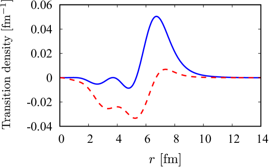
Figure 1: Transition densities for the $0^{-}$ state at $E_{0}=13.94$ MeV of ¹⁶⁰Sn. The solid (blue) and dashed (red) curves show $\rho^{\sigma}_{10}r^{3}E_{0}$ and $(\rho^{\sigma\nabla}_{0}/M)r^{2}$, respectively.

For the transition to the $1^{-}$ states, the dipole operator from the $V_{0}$ and $\bm{V}(\rm{Conv.})$ terms and the spin-dipole operator from the $\bm{A}$ term are equally important. Their contributions are shown in Tab. 2. If we do not use the current conservation relation for the convection current but use Eq. (95), the calculated decay rate becomes 140 sec^-1. The use of the current conservation relation for the electric multipole of the vector current reduces the total decay rate by about 45%, while LOB overestimates the decay rate by about 5%. The weak magnetism alters the decay rate by about 5%, which is sizable, while the contribution of the $\rho_{21}^{\nabla}$ term is less than 1%. The transition densities for the dipole and spin-dipole operators are shown in Fig. 2. One sees coherent contributions of the $V_{0}$ and $\bm{A}$ terms.

Figure 2: Transition densities for the $1^{-}$ state at $E_{0}=15.63$ MeV of ¹⁶⁰Sn. The solid (blue) and dashed (red) curves show $\rho_{1}r^{3}E_{0}$ and $\rho^{\sigma}_{11}r^{3}E_{0}$, respectively.

5 Summary

The formulas of the beta-decay rate including the velocity-dependent weak currents as well as the induced currents have been presented for the allowed and first-forbidden transitions. The longitudinal part of the vector current is eliminated by using the conservation of the vector current for the multipole operator of $P=(-1)^{J}$ transition.

The allowed and first-forbidden transitions of the beta decay of ¹⁶⁰Sn have been studied as an application of the present formulas. The transition densities are obtained by the EDF method. The results obtained with the electron wave functions in LO and NLO are compared with the ‘exact’ ones. It is shown that the conventional LO formula misses the transition rate by about 10 to 20 $\%$. Including the NLO term reproduces the ‘exact’ with high accuracy. The induced weak-magnetism term typically contributes by about a few percent to the decay rate through the interference term of the leading-order amplitude. Reorganizing the formula using the current conservation is important for the $1^{-}$ transition operator of the vector current as known well. We reconfirmed the velocity-dependent term is as equally important as the spin-dipole term for the $0^{-}$ transition. The induced pseudo-scalar term can be neglected for the nuclear beta decay.

The formulas offer semi-analytic expressions of the transition matrix element of the nuclear beta decay, which are transparent and allow us to apply not only to various beta-decay processes but also the shape and angular correlations of the beta decay and neutrino reactions. The precise formulas are also useful to search signals of BSM in nuclear beta decay.

Appendix A Nuclear matrix element

Nuclear matrix elements $w,x,u,z$ and those with Coulomb potential and velocity-dependent operators that are used in the literature are expressed in terms of the transition densities introduced in section 4:

$$w =g_{A}\sqrt{4\pi}\int_{0}^{\infty}drr^{3}\rho^{\sigma}_{10}(r),$$ (118)

$$x =\mp g_{V}\sqrt{\frac{4\pi}{3}}\int_{0}^{\infty}drr^{3}\rho_{1}(r),$$ (119)

$$u =g_{A}\sqrt{\frac{8\pi}{3}}\int_{0}^{\infty}drr^{3}\rho^{\sigma}_{11}(r),$$ (120)

$$z =-g_{A}\sqrt{\frac{16\pi}{3}}\int_{0}^{\infty}drr^{3}\rho^{\sigma}_{12}(r),$$ (121)

$$\xi w^{\prime} =g_{A}\sqrt{4\pi}\int_{0}^{\infty}drr^{2}\rho^{\sigma}_{10}(r)V_{D1}(r),$$ (122)

$$\xi x^{\prime} =\mp g_{V}\sqrt{\frac{4\pi}{3}}\int_{0}^{\infty}drr^{2}\rho_{1}(r)V_{D1}(r),$$ (123)

$$\xi u^{\prime} =g_{A}\sqrt{\frac{8\pi}{3}}\int_{0}^{\infty}drr^{2}\rho^{\sigma}_{11}(r)V_{D1}(r),$$ (124)

$$\xi^{\prime}v =\sqrt{4\pi}\frac{g_{A}}{M}\int_{0}^{\infty}drr^{2}\rho^{\sigma\nabla}_{0}(r),$$ (125)

$$\xi^{\prime}y =\mp\sqrt{4\pi}\frac{g_{V}}{M}\int_{0}^{\infty}drr^{2}\rho^{\nabla}_{01}(r),$$ (126)

$$\zeta_{0} =\xi w^{\prime}+\xi^{\prime}v+\frac{E_{0}w}{3},$$ (127)

$$\zeta_{1} =\xi^{\prime}y-\xi u^{\prime}-\xi x^{\prime}+\frac{(u-x)E_{0}}{3}$$ (128)

for $\beta^{\mp}$ decay and

$$\lambda_{2} =\frac{\alpha_{-2}^{2}+\alpha_{2}^{2}}{\alpha_{-1}^{2}+\alpha_{1}^{2}},$$ (129)

$$\frac{m_{e}}{E_{e}}\gamma_{1}\mu_{1} =\frac{\alpha_{-1}^{2}-\alpha_{1}^{2}}{\alpha_{-1}^{2}+\alpha_{1}^{2}}.$$ (130)

References

• (1) M. R. Mumpower, R. Surman, G. C. McLaughlin, and A. Aprahamian, Prog. Part. Nucl. Phys., 86, 86–126, [Erratum: Prog.Part.Nucl.Phys. 87, 116–116 (2016)] (2016), arXiv:1508.07352.
• (2) B. P. Abbott et al., Phys. Rev. Lett., 119, 161101 (2017), arXiv:1710.05832.
• (3) B. P. Abbott et al., Astrophys. J. Lett., 848, L12 (2017), arXiv:1710.05833.
• (4) G. Mention, M. Fechner, Th. Lasserre, Th. A. Mueller, D. Lhuillier, M. Cribier, and A. Letourneau, Phys. Rev. D, 83, 073006 (Apr 2011).
• (5) A. C. Hayes, J. L. Friar, G. T. Garvey, Gerard Jungman, and G. Jonkmans, Phys. Rev. Lett., 112, 202501 (May 2014).
• (6) A. Glick-Magid and D. Gazit, Jou. of Phys. G, 49(10), 105105 (sep 2022).
• (7) J. Kostensalo, M. Haaranen, and J. Suhonen, Phys. Rev. C, 95, 044313 (Apr 2017).
• (8) W. Horiuchi, T. Sato, Y. Uesaka, and K. Yoshida, Prog. Theor. Exp. Phys., 2021(10), 103D03 (2021).
• (9) K. Koshigiri, M. Nishimura, H. Ohtsubo, and M. Morita, Nucl. Phys. A, 319, 301, [Erratum: Nucl.Phys.A 340, 482 (1980)] (1979).
• (10) M. Morita and A. Fujii, Phys. Rev., 118, 606 (1960).
• (11) H. F. Schopper, Weak Interactions and Nuclear Beta Decay, (North-Holland Publishing Company, 1966).
• (12) H. Behrens and W. Bühring, Nucl. Phys. A, 162, 111–144 (1971).
• (13) I. S. Towner, Ann. Rev. Nucl. Part. Sci., 36(1), 115–136 (1986).
• (14) S. Weinberg, Phys. Rev., 112, 1375–1379 (Nov 1958).
• (15) D. H. Wilkinson, Physics Letters B, 66(2), 105–108 (1977).
• (16) J. D. Walecka, Semileptonic weak interactions in nuclei in Muon physics II, (Academic Press, Inc., 1975), Edited by V. W. Hughes and C. S. Wu.
• (17) S. Nakamura, T. Sato, Vladimir P. Gudkov, and K. Kubodera, Phys. Rev. C, 63, 034617, [Erratum: Phys.Rev.C 73, 049904 (2006)] (2001), nucl-th/0009012.
• (18) A. C. Hayes and J. L. Friar, Phys. Rev. C, 98, 065505 (Dec 2018).
• (19) A. Fujii, J.-I. Fujita, and M. Morita, Prog. Theor. Phys., 32(3), 438–449 (1964).
• (20) J.J. Sakurai and S.F. Tuan, Modern Quantum Mechanics, (Benjamin/Cummings Pub., 1985).
• (21) M. E. Rose, Elementary theory of angular momentum, (John Wiley & Sons, Inc., New York, 1957).
• (22) A.R. Edmonds, Angular Momentum in Quantum Mechanics, Investigations in Physics Series. (Princeton University Press, 1996).
• (23) T. Gorringe and H. W. Fearing, Rev. Mod. Phys., 76, 31–91 (Dec 2003).
• (24) L.D. Blokhintsev and E.I. Dolinsky, Nucl. Phys., 34(2), 498–499 (1962).
• (25) M. T. Mustonen and J. Engel, Phys. Rev. C, 93, 014304 (2016), arXiv:1510.02136.
• (26) K. Yoshida, Prog. Theor. Exp. Phys., 2013, 113D02, [Erratum: Prog. Theor. Exp. Phys., 2021, 019201 (2021)] (2013), arXiv:1308.0424.
• (27) J. Dobaczewski, H. Flocard, and J. Treiner, Nucl. Phys. A, 422, 103 – 139 (1984).
• (28) H. Kasuya and K. Yoshida, Prog. Theor. Exp. Phys., 2021, 013D01 (2021), arXiv:2005.03276.
• (29) E. Chabanat, P. Bonche, P. Haensel, J. Meyer, and R. Schaeffer, Nucl. Phys. A, 635, 231–256, [Erratum: Nucl.Phys.A 643, 441–441 (1998)] (1998).
• (30) M. Yamagami, Y. R. Shimizu, and T. Nakatsukasa, Phys. Rev. C, 80, 064301 (2009), arXiv:0812.3197.
• (31) M. Morita, Beta decay and muon capture, (Benjamin, 1973).
• (32) H. Behrens, J. Jänecke, and H. Schopper, Numerical tables for beta-decay and electron capture, (Springer-Verlag Berlin, 1969).
• (33) K. Kubodera, J. Delorme, and M. Rho, Phys. Rev. Lett., 40, 755–758 (Mar 1978).