Maxwell’s Demon for Quantum Transport
Abstract
Maxwell’s demon can be utilized to construct quantum information engines. While most of the existing quantum information engines harness thermal fluctuations, quantum information engines that utilize quantum fluctuations have recently been discussed. We propose a new type of genuinely quantum information engine that harnesses quantum fluctuations to achieve cumulative storage of useful work and unidirectional transport of a particle. Our scheme does not require thermalization, which eliminates the ambiguity in evaluating the power and velocity of our proposed engine in contrast to other existing quantum information engines that can transport a particle. We find a tradeoff relationship between the maximum achievable power and the maximum velocity. We also propose an improved definition of efficiency by clarifying all possible energy flows involved in the engine cycle.
Introduction.— A heat engine does mechanical work by harnessing thermal energy. The amount of extractable work is limited by the second law of thermodynamics. A thought experiment to overcome this limit was conceived by James Clerk Maxwell who, in modern language, realized that feedback control permits information-to-work conversion. An important application of Maxwell’s demon is to help an engine extract more work than a Carnot engine. This type of engine is called an information heat engine. A quintessential classical information heat engine is the Szilard engine Szilard (1964) which can extract work beyond the second law of thermodynamics by harnessing thermal fluctuations. Besides extracting energy and doing work in every engine cycle, one may also utilize the extracted energy cumulatively to transport a particle uphill against a potential barrier. This type of Maxwell’s-demon-assisted transport was experimentally realized with a classical Brownian particle by Toyabe et al Toyabe et al. (2010). The power and the efficiency of a heat engine, and the velocity of particle transport, have been investigated in Ref. Saha et al. (2021).
Maxwell’s demon has been extended to the quantum regime. Many types of quantum information engine have been theoretically proposed Scully et al. (2003); Kim et al. (2011); Park et al. (2013); Abah and Lutz (2014); Zhang et al. (2014); Brandner et al. (2015); Uzdin et al. (2015); Chapman and Miyake (2015); Niedenzu et al. (2016); Manzano et al. (2016); Yi et al. (2017); Elouard et al. (2017); Elouard and Jordan (2018); Ding et al. (2018); Buffoni et al. (2019); Seah et al. (2020); Auffèves (2021); Bhandari et al. (2023) and experimentally implemented Camati et al. (2016); Cottet et al. (2017); Masuyama et al. (2018); Naghiloo et al. (2018); Wang et al. (2018); Najera-Santos et al. (2020); Hernández-Gómez et al. (2022); Yan et al. (2022). However, most of them still extract work from a thermal reservoir Scully et al. (2003); Kim et al. (2011); Park et al. (2013); Abah and Lutz (2014); Zhang et al. (2014); Brandner et al. (2015); Uzdin et al. (2015); Chapman and Miyake (2015); Niedenzu et al. (2016); Manzano et al. (2016); Yi et al. (2017); Seah et al. (2020); Bhandari et al. (2023) and thermal equilibration is required for every cycle of operations. While the apparent distinction from a classical engine is that the working agent is a quantum system, it is unclear what quantum nature of the engine plays a role. Recently, quantum information engines that utilize only quantum fluctuations with no heat reservoir coupled to the working agent have been proposed Elouard et al. (2017); Auffèves (2021). The system gains energy directly from projective measurements on those observables which do not commute with the system Hamiltonian and a unit efficiency can be achieved. However, in Ref. Elouard et al. (2017), the energy extracted in one feedback loop must be released at the end of the loop to reset the engine. The lack of ability to utilize cumulatively stored energy on demand greatly limits the utility and strength of an information engine. Reference Elouard and Jordan (2018) proposes a new type of quantum information engine that can store energy and transport a particle against a potential. However, it still requires a heat bath to prepare an equilibrium state and the thermalization time is usually unknown. Therefore, it is hard to evaluate the power and the transport velocity. In this Letter, we construct a new type of quantum information engine with a tilted one-dimensional (1D) lattice that can store energy cumulatively from purely quantum fluctuations without resorting to thermalization and allows one to evaluate its power and velocity. We find that the maximum power and the maximum velocity obey a tradeoff relationship which implies that a large power can be obtained at the expense of a small velocity and vice versa. Our engine runs in pure states which are usually far from equilibrium. Transport is highly nontrivial because without Maxwell’s demon a particle in a tilted 1D lattice would undergo Bloch oscillations which are interrupted by Zener transitions Bloch (1929); Breid et al. (2006). Our information engine can transport a particle beyond the realm of Bloch oscillations without resorting to Zener transitions. We finally discuss an improved definition of the efficiency of our information engine by considering both the energy cost of measurement and that of information erasure; the former is not included in Refs. Elouard et al. (2017); Elouard and Jordan (2018); Auffèves (2021), and the later is missing in Refs. Brandner et al. (2015); Yi et al. (2017).
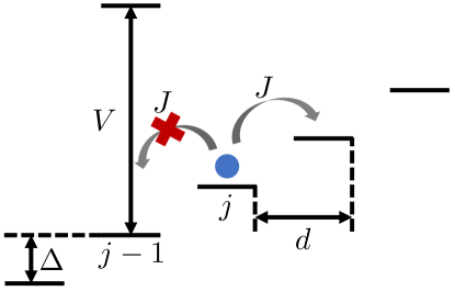
Setup.— We consider a quantum particle in a 1D ladder potential as illustrated in Fig. 1. It is described by the Wannier-Stark (WS) Hamiltonian , where is the hopping amplitude, the energy difference between two adjacent sites, the strength of the gradient force, the lattice constant, and the Wannier states. We aim at pumping up a particle against a linear potential to accumulate energy in the form of the potential energy and achieve directed motion by measurement and feedback, which is a quantum analog of Ref. Toyabe et al. (2010). We achieve this goal by the following four steps.
Step 1 – measurement: A projective position measurement is performed in the basis of Wannier states .
Step 2 – feedback control: If the particle is located at site , the potential at site is instantly raised by to prevent the particle from hopping downstairs.
Step 3 – unitary evolution: The particle undergoes a unitary evolution during time according to the Hamiltonian . A sufficiently large effectively imposes a rigid wall at site such that for . The effective Hamiltonian is then given by
| (1) |
where the upper limit of the summation is truncated because a long but finite chain with sites is used in numerical simulations. This truncation is valid if during the simulation where the time-evolved state is .
Step 4 – information erasure: We erase the information of measurement outcomes that is stored in the memory of the probe and start the next cycle.
We are interested in the average rate of energy storage (power ), the average rate of particle transport (velocity ), and the efficiency which will be defined later. We first demonstrate that the average power in a long time is defined by where is the average energy stored in one feedback loop. We consider a trajectory of feedback loops with the total time . The total accumulated energy gain is , where is the energy stored in the th loop which is a stochastic variable. The power for this trajectory is given by . In the limit of , the power converges to , where the law of large numbers is used to obtain .
Let us introduce a rescaled gradient and time . The dimensionless Hamiltonian is , and the average stored energy is , where is the probability of measurement outcome . The dimensionless energy gain is . We define the dimensionless power to be . The average velocity is defined as the number of traveled sites per second . Therefore, the dimensionless velocity is . The maximum power and velocity share the same optimal time for a fixed value of . We first present numerical results.
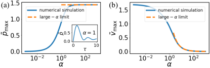
Results.— In Fig. 2, we plot the maximum power (a) and the maximum velocity (b) achievable by changing for each value of . The blue curves show numerical results. The maximum power exhibits a monotonic increase with increasing , and an opposite trend is seen for the maximum velocity, indicating a tradeoff relationship between the maximum power and the maximum velocity. To achieve a large power, a large gradient should be used, which suppresses the velocity; conversely, to achieve a large velocity, the gradient should be made small, which reduces the power.
Let us analyze the two limiting cases.
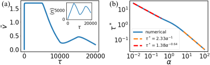
Small- regime. For , the maximally achievable power approaches zero and the maximum velocity saturates to a constant value. To understand the saturation constant for the velocity, we consider a flat lattice in the limit and assume that the particle is initially at site with a rigid wall placed at . After a short transient dynamics, the wave packet of the particle travels in the right direction with a constant velocity [see Fig. 3(a)]. For a semi-infinite chain, the velocity is kept constant. For a finite chain as used in the numerical simulation, the right boundary will eventually reflect the wave packet to decrease the velocity. The physics underlying the value of this constant velocity can be qualitatively understood from Heisenberg’s uncertainty principle. Since the particle is initially localized at site 1, the momentum fluctuates due to Heisenberg’s uncertainty relation, providing the energy for the particle to move to the right. Because the expectation value of the kinetic energy for the initial state is 0, the variance of it is . Its standard deviation is . The velocity is then expected to be with being the effective mass. This value is close to the numerically obtained result of 1.7. For a finite , the average velocity multiplied by gives the power, which makes the maximum power vanish in the small- regime.
Large- regime. For , the dynamics is effectively confined within neighboring sites which are described by a two-dimensional Hilbert space. This approximation allows exact calculations by using an effective Hamiltonian . The leading two terms of energy gain within time are . The maximum value is obtained for the running time with . The power is given by
| (2) |
The maximum value is independent of and close to at , which is consistent with the numerical results as plotted in Figs. 2(a) and 3(b). As increases, the maximum velocity decreases as as shown in Fig. 2(b).
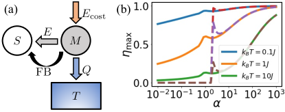
Efficiency.— Another important measure for an engine is efficiency. For a classical heat engine, the efficiency is defined as the work output by the working agent divided by the heat absorbed from the hot heat bath. Following this logic, we clarify the energy flow involved in our engine and define the efficiency [see Fig. 4(a)]. There are two steps involving energy inputs. First, during the unitary evolution, the kinetic energy is converted to the potential energy. Then the quantum measurement increases the internal energy of the particle [ in Fig. 4(a)] by which compensates for a decrease in the kinetic energy, and a correlation between the probe and the particle is established. This quantum measurement requires an energy input , which is especially important for a quantum system because quantum measurement may directly alter the energy. We assume that applying the feedback control protocol, i.e., raising a potential, is ideal and cost-free. This assumption has widely been made in the context of Maxwell’s demon Sagawa and Ueda (2008, 2009, 2011); Bhandari et al. (2023); Parrondo et al. (2015); Elouard and Jordan (2018); Auffèves (2021). The second step is information erasure. To start the next cycle, the information stored in the measurement probe must be discarded in contact with a heat bath with temperature . This requires an amount of energy according to Landauer’s principle Landauer (1961); Bennett (1982). Therefore, the energy resource required for our engine is given by . There is no fundamental limit to the energy cost of each individual process of measurement and erasure. However, there exists a fundamental bound on the total energy cost Sagawa and Ueda (2009, 2011). In Refs. Elouard et al. (2017); Elouard and Jordan (2018); Auffèves (2021), is not included in the resource, and in Refs. Brandner et al. (2015); Yi et al. (2017), is not considered. For example, in Refs. Elouard et al. (2017); Elouard and Jordan (2018); Auffèves (2021), the efficiency is defined as without . However, information erasure can, in principle, be performed without work Sagawa and Ueda (2009), which makes it possible to achieve regardless of details of the engine. We, therefore, define the efficiency of our quantum information engine as
| (3) |
This total energy cost can be calculated using standard techniques in information thermodynamics Jacobs (2009); Sagawa and Ueda (2009, 2011); Jacobs (2012); Faist et al. (2015); Abdelkhalek et al. (2016); Deffner et al. (2016); Mohammady (2021). The total energy cost considered here includes both heat and work because it is difficult to make a clear-cut distinction about the form of the energy for a quantum system. This, on the other hand, allows one to obtain an equality for this cost, rather than an inequality for heat or work alone. For projective measurements, the total energy cost is Abdelkhalek et al. (2016)
| (4) |
where is an internal energy change in the system due to the quantum measurement, is the temperature of the heat bath coupled to the probe, and is the Shannon entropy of the measurement outcomes . Because the Shannon entropy is positive for any nonzero time , the efficiency is bound within . We note that we cannot simply replace by in defined in Refs. Elouard et al. (2017); Elouard and Jordan (2018); Auffèves (2021) to make the definition of the efficiency complete since we would then have a negative efficiency. With the proposed new definition (3), such a problem is circumvented and the efficiencies for the engines in Refs. Elouard et al. (2017); Elouard and Jordan (2018); Auffèves (2021) are again bounded within . The values of the optimal efficiencies and the required conditions also remain the same.
We now examine the behavior of the maximally achievable efficiency plotted in Fig. 4(b). The numerically obtained curves increase almost monotonically with increasing , except for a small bump in the middle. As the gradient becomes steeper, the maximum efficiency increases and becomes closer to unity. The efficiency in this large- regime can analytically be calculated to be
| (5) |
where . It is clear that for a fixed , the maximum is obtained at with which agrees with the optimal time for energy gain. The maximum efficiency is given by
| (6) |
which approaches unity for large because . This possible unity efficiency is similar to the engines discussed in Refs. Elouard et al. (2017); Elouard and Jordan (2018). The reason is that the Shannon entropy of measurement outcomes is so small that little heat is dissipated into the environment. Almost all of the energy input is converted into the potential energy of the particle.
Discussions.— Our engine possesses several unique features and advantages compared with other information engines. First, it has a well-defined finite optimal time according to the task [see Fig. 3(b)], which is beneficial to experiments and performance evaluation, while the thermalization time is unspecified in Ref. Elouard and Jordan (2018). The optimal time is basically of the order of the Bloch oscillation period due to the competition between hopping to the right by and reflection by . This makes a sharp contrast with the cases in Refs. Elouard et al. (2017); Saha et al. (2021) where the maximum values are attained within a vanishingly short time.
Second, we find a crucial dependence on the gradient which was not analyzed in the continuous-space linear engine in Ref. Elouard and Jordan (2018). The power-velocity tradeoff relationship can guide experimentalists in tuning gradient and evolution time. For example, to have the largest maximum power, one needs to use a relatively large gradient, meaning a short evolution time which may also be advantageous experimentally because a shorter implementation time means less decoherence.
Another advantage of this engine is that every step in the engine cycle can be implemented with existing experimental techniques. The Hamiltonian may be experimentally realized with an ultracold atom in an optical lattice Preiss et al. (2015); Ueda (2020) or a qubit in a superconducting quantum processor Guo et al. (2021). The projective position measurement with the single-site resolution can be achieved by quantum gas microscopy Bakr et al. (2009); Sherson et al. (2010); Haller et al. (2015); Cheuk et al. (2015); Parsons et al. (2015); Yamamoto et al. (2017); Okuno et al. (2020); Yamamoto et al. (2020) and the single-site addressing Weitenberg et al. (2011); Viscor et al. (2012); Fukuhara et al. (2013); Wang et al. (2015); Zupancic et al. (2016); Koepsell et al. (2019); Ji et al. (2021) might be used to perform the feedback control.
A single particle on an infinite 1D tilted lattice can only oscillate within a constrained range around the initial position due to Bloch oscillations Bloch (1929); Hartmann et al. (2004). This is in stark contrast to the classical case where the particle tends to move downstairs due to a potential gradient Toyabe et al. (2010) and the quantum continuous-space linear potential where no Bloch oscillation occurs Gea-Banacloche (1999); Vallée (2000); Elouard and Jordan (2018). However, by measurement and feedback control, we can achieve a finite velocity of unidirectional motion even for a long time. We can transport a particle beyond the realm of Bloch oscillations without resorting to Zener transitions.
Outlook.— In this work, we have only used projective measurements. It is interesting to continuously monitor the dynamics Ashida and Ueda (2017); Bernard et al. (2018); Ashida (2020); Manzano and Zambrini (2022); Belenchia et al. (2020); Yada et al. (2022) and apply feedback control constantly as done classically Saha et al. (2021). We have also assumed cost-free feedback control. However, in modeling the feedback controller Ehrich et al. (2022) or when the feedback protocol inevitably alters the quantum state Kim et al. (2011), the energy flow due to feedback control should also be considered. Another interesting direction is to investigate fundamental bounds on the performance of our engine Barato and Seifert (2015); Pietzonka and Seifert (2018); Liu et al. (2020); Gong and Hamazaki (2022); Hamazaki (2022).
Acknowledgements.
We acknowledge David A. Sivak, Shoki Sugimoto, and Koki Shiraishi for fruitful discussions. K.L. is supported by the Global Science Graduate Course (GSGC) program of the University of Tokyo. M.N. is supported by JSPS KAKENHI Grant No. JP20K14383. M.U. is supported by KAKENHI Grant No. JP22H01152 from the Japan Society for the Promotion of Science.References
- Szilard (1964) Leo Szilard, “On the decrease of entropy in a thermodynamic system by the intervention of intelligent beings,” Behav. Sci. 9, 301–310 (1964).
- Toyabe et al. (2010) Shoichi Toyabe, Takahiro Sagawa, Masahito Ueda, Eiro Muneyuki, and Masaki Sano, “Experimental demonstration of information-to-energy conversion and validation of the generalized jarzynski equality,” Nat. Phys. 6, 988–992 (2010).
- Saha et al. (2021) Tushar K. Saha, Joseph N. E. Lucero, Jannik Ehrich, David A. Sivak, and John Bechhoefer, “Maximizing power and velocity of an information engine,” Proc. Natl. Acad. Sci. U.S.A. 118 (2021).
- Scully et al. (2003) Marlan O. Scully, M. Suhail Zubairy, Girish S. Agarwal, and Herbert Walther, “Extracting work from a single heat bath via vanishing quantum coherence,” Science 299, 862–864 (2003).
- Kim et al. (2011) Sang Wook Kim, Takahiro Sagawa, Simone De Liberato, and Masahito Ueda, “Quantum szilard engine,” Phys. Rev. Lett. 106, 070401 (2011).
- Park et al. (2013) Jung Jun Park, Kang-Hwan Kim, Takahiro Sagawa, and Sang Wook Kim, “Heat engine driven by purely quantum information,” Phys. Rev. Lett. 111, 230402 (2013).
- Abah and Lutz (2014) Obinna Abah and Eric Lutz, “Efficiency of heat engines coupled to nonequilibrium reservoirs,” EPL 106, 20001 (2014).
- Zhang et al. (2014) Keye Zhang, Francesco Bariani, and Pierre Meystre, “Quantum optomechanical heat engine,” Phys. Rev. Lett. 112, 150602 (2014).
- Brandner et al. (2015) Kay Brandner, Michael Bauer, Michael T Schmid, and Udo Seifert, “Coherence-enhanced efficiency of feedback-driven quantum engines,” New J. Phys. 17, 065006 (2015).
- Uzdin et al. (2015) Raam Uzdin, Amikam Levy, and Ronnie Kosloff, “Equivalence of quantum heat machines, and quantum-thermodynamic signatures,” Phys. Rev. X 5, 031044 (2015).
- Chapman and Miyake (2015) Adrian Chapman and Akimasa Miyake, “How an autonomous quantum maxwell demon can harness correlated information,” Phys. Rev. E 92, 062125 (2015).
- Niedenzu et al. (2016) Wolfgang Niedenzu, David Gelbwaser-Klimovsky, Abraham G Kofman, and Gershon Kurizki, “On the operation of machines powered by quantum non-thermal baths,” New J. Phys. 18, 083012 (2016).
- Manzano et al. (2016) Gonzalo Manzano, Fernando Galve, Roberta Zambrini, and Juan M. R. Parrondo, “Entropy production and thermodynamic power of the squeezed thermal reservoir,” Phys. Rev. E 93, 052120 (2016).
- Yi et al. (2017) Juyeon Yi, Peter Talkner, and Yong Woon Kim, “Single-temperature quantum engine without feedback control,” Phys. Rev. E 96, 022108 (2017).
- Elouard et al. (2017) Cyril Elouard, David Herrera-Martí, Benjamin Huard, and Alexia Auffèves, “Extracting work from quantum measurement in maxwell’s demon engines,” Phys. Rev. Lett. 118, 260603 (2017).
- Elouard and Jordan (2018) Cyril Elouard and Andrew N. Jordan, “Efficient quantum measurement engines,” Phys. Rev. Lett. 120, 260601 (2018).
- Ding et al. (2018) Xuehao Ding, Juyeon Yi, Yong Woon Kim, and Peter Talkner, “Measurement-driven single temperature engine,” Phys. Rev. E 98, 042122 (2018).
- Buffoni et al. (2019) Lorenzo Buffoni, Andrea Solfanelli, Paola Verrucchi, Alessandro Cuccoli, and Michele Campisi, “Quantum measurement cooling,” Phys. Rev. Lett. 122, 070603 (2019).
- Seah et al. (2020) Stella Seah, Stefan Nimmrichter, and Valerio Scarani, “Maxwell’s lesser demon: A quantum engine driven by pointer measurements,” Phys. Rev. Lett. 124, 100603 (2020).
- Auffèves (2021) Alexia Auffèves, “A short story of quantum and information thermodynamics,” SciPost Phys. Lect. Notes , 27 (2021).
- Bhandari et al. (2023) Bibek Bhandari, Robert Czupryniak, Paolo Andrea Erdman, and Andrew N. Jordan, “Measurement-based quantum thermal machines with feedback control,” Entropy 25, 204 (2023).
- Camati et al. (2016) Patrice A. Camati, John P. S. Peterson, Tiago B. Batalhão, Kaonan Micadei, Alexandre M. Souza, Roberto S. Sarthour, Ivan S. Oliveira, and Roberto M. Serra, “Experimental rectification of entropy production by maxwell’s demon in a quantum system,” Phys. Rev. Lett. 117, 240502 (2016).
- Cottet et al. (2017) Nathanaël Cottet, Sébastien Jezouin, Landry Bretheau, Philippe Campagne-Ibarcq, Quentin Ficheux, Janet Anders, Alexia Auffèves, Rémi Azouit, Pierre Rouchon, and Benjamin Huard, “Observing a quantum maxwell demon at work,” Proc. Natl. Acad. Sci. U.S.A. 114, 7561–7564 (2017).
- Masuyama et al. (2018) Y. Masuyama, K. Funo, Y. Murashita, A. Noguchi, S. Kono, Y. Tabuchi, R. Yamazaki, M. Ueda, and Y. Nakamura, “Information-to-work conversion by maxwell’s demon in a superconducting circuit quantum electrodynamical system,” Nat. Commun. 9, 1291 (2018).
- Naghiloo et al. (2018) M. Naghiloo, J. J. Alonso, A. Romito, E. Lutz, and K. W. Murch, “Information gain and loss for a quantum maxwell’s demon,” Phys. Rev. Lett. 121, 030604 (2018).
- Wang et al. (2018) W.-B. Wang, X.-Y. Chang, F. Wang, P.-Y. Hou, Y.-Y. Huang, W.-G. Zhang, X.-L. Ouyang, X.-Z. Huang, Z.-Y. Zhang, H.-Y. Wang, L. He, and L.-M. Duan, “Realization of quantum maxwell’s demon with solid-state spins*,” Chin. Phys. Lett. 35, 040301 (2018).
- Najera-Santos et al. (2020) Baldo-Luis Najera-Santos, Patrice A. Camati, Valentin Métillon, Michel Brune, Jean-Michel Raimond, Alexia Auffèves, and Igor Dotsenko, “Autonomous maxwell’s demon in a cavity qed system,” Phys. Rev. Res. 2, 032025 (2020).
- Hernández-Gómez et al. (2022) S. Hernández-Gómez, S. Gherardini, N. Staudenmaier, F. Poggiali, M. Campisi, A. Trombettoni, F.S. Cataliotti, P. Cappellaro, and N. Fabbri, “Autonomous dissipative maxwell’s demon in a diamond spin qutrit,” PRX Quantum 3, 020329 (2022).
- Yan et al. (2022) Lei-Lei Yan, Lv-Yun Wang, Shi-Lei Su, Fei Zhou, and Mang Feng, “Verification of information thermodynamics in a trapped ion system,” Entropy 24, 813 (2022).
- Bloch (1929) Felix Bloch, “Über die quantenmechanik der elektronen in kristallgittern,” Z. Phys. 52, 555–600 (1929).
- Breid et al. (2006) B M Breid, D Witthaut, and H J Korsch, “Bloch–zener oscillations,” New J. Phys. 8, 110 (2006).
- Sagawa and Ueda (2008) Takahiro Sagawa and Masahito Ueda, “Second law of thermodynamics with discrete quantum feedback control,” Phys. Rev. Lett. 100, 080403 (2008).
- Sagawa and Ueda (2009) Takahiro Sagawa and Masahito Ueda, “Minimal energy cost for thermodynamic information processing: Measurement and information erasure,” Phys. Rev. Lett. 102, 250602 (2009).
- Sagawa and Ueda (2011) Takahiro Sagawa and Masahito Ueda, “Erratum: Minimal energy cost for thermodynamic information processing: Measurement and information erasure [phys. rev. lett. 102, 250602 (2009)],” Phys. Rev. Lett. 106, 189901 (2011).
- Parrondo et al. (2015) Juan M. R. Parrondo, Jordan M. Horowitz, and Takahiro Sagawa, “Thermodynamics of information,” Nat. Phys 11, 131–139 (2015).
- Landauer (1961) R. Landauer, “Irreversibility and heat generation in the computing process,” IBM J. Res. Dev. 5, 183–191 (1961).
- Bennett (1982) Charles H. Bennett, “The thermodynamics of computation—a review,” Int. J. Theor. Phys. 21, 905–940 (1982).
- Jacobs (2009) Kurt Jacobs, “Second law of thermodynamics and quantum feedback control: Maxwell’s demon with weak measurements,” Phys. Rev. A 80, 012322 (2009).
- Jacobs (2012) Kurt Jacobs, “Quantum measurement and the first law of thermodynamics: The energy cost of measurement is the work value of the acquired information,” Phys. Rev. E 86, 040106 (2012).
- Faist et al. (2015) Philippe Faist, Frédéric Dupuis, Jonathan Oppenheim, and Renato Renner, “The minimal work cost of information processing,” Nat. Commun. 6, 7669 (2015).
- Abdelkhalek et al. (2016) Kais Abdelkhalek, Yoshifumi Nakata, and David Reeb, “Fundamental energy cost for quantum measurement,” (2016).
- Deffner et al. (2016) Sebastian Deffner, Juan Pablo Paz, and Wojciech H. Zurek, “Quantum work and the thermodynamic cost of quantum measurements,” Phys. Rev. E 94, 010103 (2016).
- Mohammady (2021) M. Hamed Mohammady, “Classicality of the heat produced by quantum measurements,” Phys. Rev. A 104, 062202 (2021).
- Preiss et al. (2015) Philipp M. Preiss, Ruichao Ma, M. Eric Tai, Alexander Lukin, Matthew Rispoli, Philip Zupancic, Yoav Lahini, Rajibul Islam, and Markus Greiner, “Strongly correlated quantum walks in optical lattices,” Science 347, 1229–1233 (2015).
- Ueda (2020) Masahito Ueda, “Quantum equilibration, thermalization and prethermalization in ultracold atoms,” Nat. Rev. Phys. 2, 669–681 (2020).
- Guo et al. (2021) Xue-Yi Guo, Zi-Yong Ge, Hekang Li, Zhan Wang, Yu-Ran Zhang, Pengtao Song, Zhongcheng Xiang, Xiaohui Song, Yirong Jin, Li Lu, Kai Xu, Dongning Zheng, and Heng Fan, “Observation of bloch oscillations and wannier-stark localization on a superconducting quantum processor,” Npj Quantum Inf. 7, 51 (2021).
- Bakr et al. (2009) Waseem S. Bakr, Jonathon I. Gillen, Amy Peng, Simon Fölling, and Markus Greiner, “A quantum gas microscope for detecting single atoms in a hubbard-regime optical lattice,” Nature 462, 74–77 (2009).
- Sherson et al. (2010) Jacob F. Sherson, Christof Weitenberg, Manuel Endres, Marc Cheneau, Immanuel Bloch, and Stefan Kuhr, “Single-atom-resolved fluorescence imaging of an atomic mott insulator,” Nature 467, 68–72 (2010).
- Haller et al. (2015) Elmar Haller, James Hudson, Andrew Kelly, Dylan A. Cotta, Bruno Peaudecerf, Graham D. Bruce, and Stefan Kuhr, “Single-atom imaging of fermions in a quantum-gas microscope,” Nat. Phys. 11, 738–742 (2015).
- Cheuk et al. (2015) Lawrence W. Cheuk, Matthew A. Nichols, Melih Okan, Thomas Gersdorf, Vinay V. Ramasesh, Waseem S. Bakr, Thomas Lompe, and Martin W. Zwierlein, “Quantum-gas microscope for fermionic atoms,” Phys. Rev. Lett. 114, 193001 (2015).
- Parsons et al. (2015) Maxwell F. Parsons, Florian Huber, Anton Mazurenko, Christie S. Chiu, Widagdo Setiawan, Katherine Wooley-Brown, Sebastian Blatt, and Markus Greiner, “Site-resolved imaging of fermionic in an optical lattice,” Phys. Rev. Lett. 114, 213002 (2015).
- Yamamoto et al. (2017) Ryuta Yamamoto, Jun Kobayashi, Kohei Kato, Takuma Kuno, Yuto Sakura, and Yoshiro Takahashi, “Site-resolved imaging of single atoms with a faraday quantum gas microscope,” Phys. Rev. A 96, 033610 (2017).
- Okuno et al. (2020) Daichi Okuno, Yoshiki Amano, Katsunari Enomoto, Nobuyuki Takei, and Yoshiro Takahashi, “Schemes for nondestructive quantum gas microscopy of single atoms in an optical lattice,” New J. Phys. 22, 013041 (2020).
- Yamamoto et al. (2020) Ryuta Yamamoto, Hideki Ozawa, David C. Nak, Ippei Nakamura, and Takeshi Fukuhara, “Single-site-resolved imaging of ultracold atoms in a triangular optical lattice,” New J. Phys. 22, 123028 (2020).
- Weitenberg et al. (2011) Christof Weitenberg, Manuel Endres, Jacob F. Sherson, Marc Cheneau, Peter Schauß, Takeshi Fukuhara, Immanuel Bloch, and Stefan Kuhr, “Single-spin addressing in an atomic mott insulator,” Nature 471, 319–324 (2011).
- Viscor et al. (2012) D. Viscor, J. L. Rubio, G. Birkl, J. Mompart, and V. Ahufinger, “Single-site addressing of ultracold atoms beyond the diffraction limit via position-dependent adiabatic passage,” Phys. Rev. A 86, 063409 (2012).
- Fukuhara et al. (2013) Takeshi Fukuhara, Adrian Kantian, Manuel Endres, Marc Cheneau, Peter Schauß, Sebastian Hild, David Bellem, Ulrich Schollwöck, Thierry Giamarchi, Christian Gross, Immanuel Bloch, and Stefan Kuhr, “Quantum dynamics of a mobile spin impurity,” Nat. Phys. 9, 235–241 (2013).
- Wang et al. (2015) Yang Wang, Xianli Zhang, Theodore A. Corcovilos, Aishwarya Kumar, and David S. Weiss, “Coherent addressing of individual neutral atoms in a 3d optical lattice,” Phys. Rev. Lett. 115, 043003 (2015).
- Zupancic et al. (2016) Philip Zupancic, Philipp M. Preiss, Ruichao Ma, Alexander Lukin, M. Eric Tai, Matthew Rispoli, Rajibul Islam, and Markus Greiner, “Ultra-precise holographic beam shaping for microscopic quantum control,” Opt. Express 24, 13881–13893 (2016).
- Koepsell et al. (2019) Joannis Koepsell, Jayadev Vijayan, Pimonpan Sompet, Fabian Grusdt, Timon A. Hilker, Eugene Demler, Guillaume Salomon, Immanuel Bloch, and Christian Gross, “Imaging magnetic polarons in the doped fermi–hubbard model,” Nature 572, 358–362 (2019).
- Ji et al. (2021) Geoffrey Ji, Muqing Xu, Lev Haldar Kendrick, Christie S. Chiu, Justus C. Brüggenjürgen, Daniel Greif, Annabelle Bohrdt, Fabian Grusdt, Eugene Demler, Martin Lebrat, and Markus Greiner, “Coupling a mobile hole to an antiferromagnetic spin background: Transient dynamics of a magnetic polaron,” Phys. Rev. X 11, 021022 (2021).
- Hartmann et al. (2004) T Hartmann, F Keck, H J Korsch, and S Mossmann, “Dynamics of bloch oscillations,” New J. Phys. 6, 2–2 (2004).
- Gea-Banacloche (1999) Julio Gea-Banacloche, “A quantum bouncing ball,” Am. J. Phys. 67, 776–782 (1999).
- Vallée (2000) Olivier Vallée, “Comment on “a quantum bouncing ball,” by julio gea-banacloche [am. j. phys. 67 (9), 776–782 (1999)],” Am. J. Phys. 68, 672–673 (2000).
- Ashida and Ueda (2017) Yuto Ashida and Masahito Ueda, “Multiparticle quantum dynamics under real-time observation,” Phys. Rev. A 95, 022124 (2017).
- Bernard et al. (2018) D. Bernard, T. Jin, and O. Shpielberg, “Transport in quantum chains under strong monitoring,” EPL 121, 60006 (2018).
- Ashida (2020) Yuto Ashida, “Continuous observation of quantum systems,” in Quantum Many-Body Physics in Open Systems: Measurement and Strong Correlations (Springer Singapore, Singapore, 2020) pp. 13–28.
- Manzano and Zambrini (2022) Gonzalo Manzano and Roberta Zambrini, “Quantum thermodynamics under continuous monitoring: A general framework,” AVS Quantum Science 4, 025302 (2022).
- Belenchia et al. (2020) Alessio Belenchia, Luca Mancino, Gabriel T. Landi, and Mauro Paternostro, “Entropy production in continuously measured gaussian quantum systems,” Npj Quantum Inf. 6, 97 (2020).
- Yada et al. (2022) Toshihiro Yada, Nobuyuki Yoshioka, and Takahiro Sagawa, “Quantum fluctuation theorem under quantum jumps with continuous measurement and feedback,” Phys. Rev. Lett. 128, 170601 (2022).
- Ehrich et al. (2022) Jannik Ehrich, Susanne Still, and David A. Sivak, “Energetic cost of feedback control,” (2022).
- Barato and Seifert (2015) Andre C. Barato and Udo Seifert, “Thermodynamic uncertainty relation for biomolecular processes,” Phys. Rev. Lett. 114, 158101 (2015).
- Pietzonka and Seifert (2018) Patrick Pietzonka and Udo Seifert, “Universal trade-off between power, efficiency, and constancy in steady-state heat engines,” Phys. Rev. Lett. 120, 190602 (2018).
- Liu et al. (2020) Kangqiao Liu, Zongping Gong, and Masahito Ueda, “Thermodynamic uncertainty relation for arbitrary initial states,” Phys. Rev. Lett. 125, 140602 (2020).
- Gong and Hamazaki (2022) Zongping Gong and Ryusuke Hamazaki, “Bounds in nonequilibrium quantum dynamics,” Int. J. Mod. Phys. B 36, 2230007 (2022).
- Hamazaki (2022) Ryusuke Hamazaki, “Speed limits for macroscopic transitions,” PRX Quantum 3, 020319 (2022).