Determining Aperture Field for Arbitrary Phaseless Far-Field Utilizing Inverse Design Method Based on Spectral Analysis

Abstract

In this communication, we propose an inverse design method based on spectral analysis (IDMBSA) for achieving desired far-field radiation pattern through aperture field design. The aperture field obtained through IDMBSA can be utilized for array synthesis and sparse array design, and it can also serve as a design objective for existing aperture field implementation methods. IDMBSA combined with the coordinate transformation enables the fulfillment of design requirements for arbitrary phaseless radiation pattern and polarization needs. Non-linearity introduced by phaseless is addressed with a multi-objective optimization (MOO) algorithm. Compared to traditional array synthesis methods, IDMBSA significantly reduces the number of optimization variables by using modal expansion and further reduces the computational burden by utilizing analytical solutions. The inherent smoothness of the aperture field obtained through IDMBSA allows for direct application in existing aperture field implementation methods, facilitating the direct design of radiating devices with arbitrary far-field radiation pattern. Simulations were conducted to explore IDMBSA’s application in array synthesis, sparse arrays, and dual-polarization independent design, the results show the practicability of IDMBSA and its wide application prospect.

I Introduction

The radiation pattern is a crucial parameter in antenna systems and is a hot spot for scholars’ research. Its requirements depend on the application scenarios and performance needs. Researchers have explored several approaches to shape the radiation pattern. One is to utilize array synthesis techniques to obtain the amplitude and phase information of each element’s feeding signal, and then implement it through the array antenna[1, 2, 3, 4, 5, 6, 7, 8, 9], typically with element spacing close to half a wavelength. With the development of metamaterial, array with sub-wavelength unit cell have gradually been widely used. Researchers directly design antennas that meet specific requirements, such as transmit arrays, reflect arrays[10], and metasurface antennas[11, 12]. Further, the device design methods which directly target the aperture field [13, 14], have gradually received attention from scholars.

Among early efforts in array synthesis, several effective methodologies were introduced by [1, 2], establishing the foundation for addressing array synthesis. Furthermore, Bucci and colleagues extended the work by using a generalized projection algorithm to reduce the possibility of the synthesis algorithm being trapped by spurious solutions in a subsequent publication [3]. With the increasing computational capabilities of computers, Multi-Objective Optimization (MOO) algorithms, such as Particle Swarm Optimization (PSO) [15, 16] and Genetic Algorithms (GA)[17] have found applications in array synthesis[5, 4, 7, 6]. Array synthesis techniques often require simultaneous optimization of both amplitudes and phases of elements, and sometimes only phase optimization is required [7]. This presents a significant challenge due to the notable increase in the dimensionality of the solution space as the number of elements grows [8, 7, 6]. For instance, to optimize the feed phase for an array with the electrical size of $17\lambda$, [6] utilizes PSO to search solutions in the 848-dimensional solution hyperspace. [9] proposes a method to reduce the number of variables using irregular arrays, but the method is only applicable when maximizing directivity is desired. Furthermore, due to the independence of optimization variables in array synthesis, there can be cases where adjacent elements have similar excitation amplitudes but opposite phases, which leads to increased discrepancies between simulation and measurement results.

The popularization of arrays featuring sub-wavelength unit cells, such as metaantennas, has drawn the focus of scholars toward novel methodologies. [18] introduces a procedure for solving non-convex array synthesis problems, which is based on the semidefinite relaxation (SDR) technique. [12] addresses the smooth-phase constraint to reduce the influence of the aperiodic arrangement of elements, and utilizes the alternating direction method of multipliers (ADMM) to achieve the synthesis of the Huygens metasurface.

With the rise of metamaterial and metaantennas, scholars have shown interest in integrating array synthesis techniques with metasurface design to achieve a one-stop design. For example, in [19], designers solve for the surface parameters based on their application-specific far-field criteria. Furthermore, [13] focuses on the design of tensorial modulated metasurfaces able to implement arbitrary aperture field distributions. [14] presents a design procedure for cavity-excited omega-bianisotropic metasurfaces generating desirable field distribution on their aperture.

[13] and [14] demonstrate the feasibility of achieving arbitrary aperture field and emphasize the significance of continuous aperture fields. The methods to obtain aperture fields from the far-field and near-field are indispensable. However, [13] and [14] do not discuss how to design the aperture field on demand. The authors of [13] put forward a method to derive the aperture fields generating the required near-field radiation in [20]. Similarly, we presented a method for converting port field distribution into a device’s internal field distribution using time-reversal techniques in [21].

This communication proposes an inverse design method based on spectral analysis (IDMBSA) to determine aperture field from arbitrary phaseless far-field radiation pattern (phaseless but with polarization information). IDMBSA has broad prospects for application, as it can be utilized to provide on-demand aperture field distribution for physical implementation methods like [13] and [14]. It naturally adapts to the polarization constraint and also can be used to overcome the drawback of excessive optimization variables in existing array synthesis methods such as [7, 6, 8]. IDMBSA is also applicable to sparse array design and can independently design the radiation patterns for different polarizations.

Specifically, by integrating the far-field asymptotic solution of the spectral domain method and employing analytic integration, IDMBSA successfully alleviates computational burden compared to [22]. IDMBSA utilizes modal expansion [23] to effectively reduce the number of optimization variables while ensuring the smoothness of the aperture field results, which is beneficial for physical implementation. Lastly, PSO [15, 16] is employed to determine the modal coefficients and obtain the aperture field. Additionally, IDMBSA combined with the Ludwig3 coordinate transformation [24] enables the fulfillment of design requirements for arbitrary radiation pattern and polarization needs.

The rest of this communication is presented as follows. Section II provides the background of the problem. Section III presents the inverse design method, including the specific derivation and solution process. In section IV, numerical simulations of aperture field obtained using IDMBSA are given, and verified by full-wave simulation experiments. In Section V, we present multiple cases to demonstrate the practicality of IDMBSA in array synthesis, sparse arrays, independent design for two polarizations, and so on.

II Background

The general aperture radiation problem is calculating the radiation field from the known aperture field $\boldsymbol{E}_{\mathrm{ape}}(x,y)|_{z=0}$. Its schematic diagram is shown in Fig. 1. The analysis below consider only the upper half-space ($z>0$), that is $\theta\in[0,{\pi}/{2}]$. The aperture field $\boldsymbol{E}_{\mathrm{ape}}$, defined over the domain $\left\{(x,y)\,|\,x\in[-\frac{a}{2},\frac{a}{2}],y\in[-\frac{b}{2},\frac{b}{2}]\right\}$, is mounted on an infinite ground plane (PEC) located at $z=0$. According to the uniqueness theorem, as long as the tangential components of $\boldsymbol{E}_{\mathrm{ape}}(x,y)$ ($E_{\mathrm{ape},x}$ and $E_{\mathrm{ape},y}$) are known, $\boldsymbol{E}(x,y,z)|_{z>0}$ is uniquely determined. This forward problem can be analyzed in spatial or spectral domains.

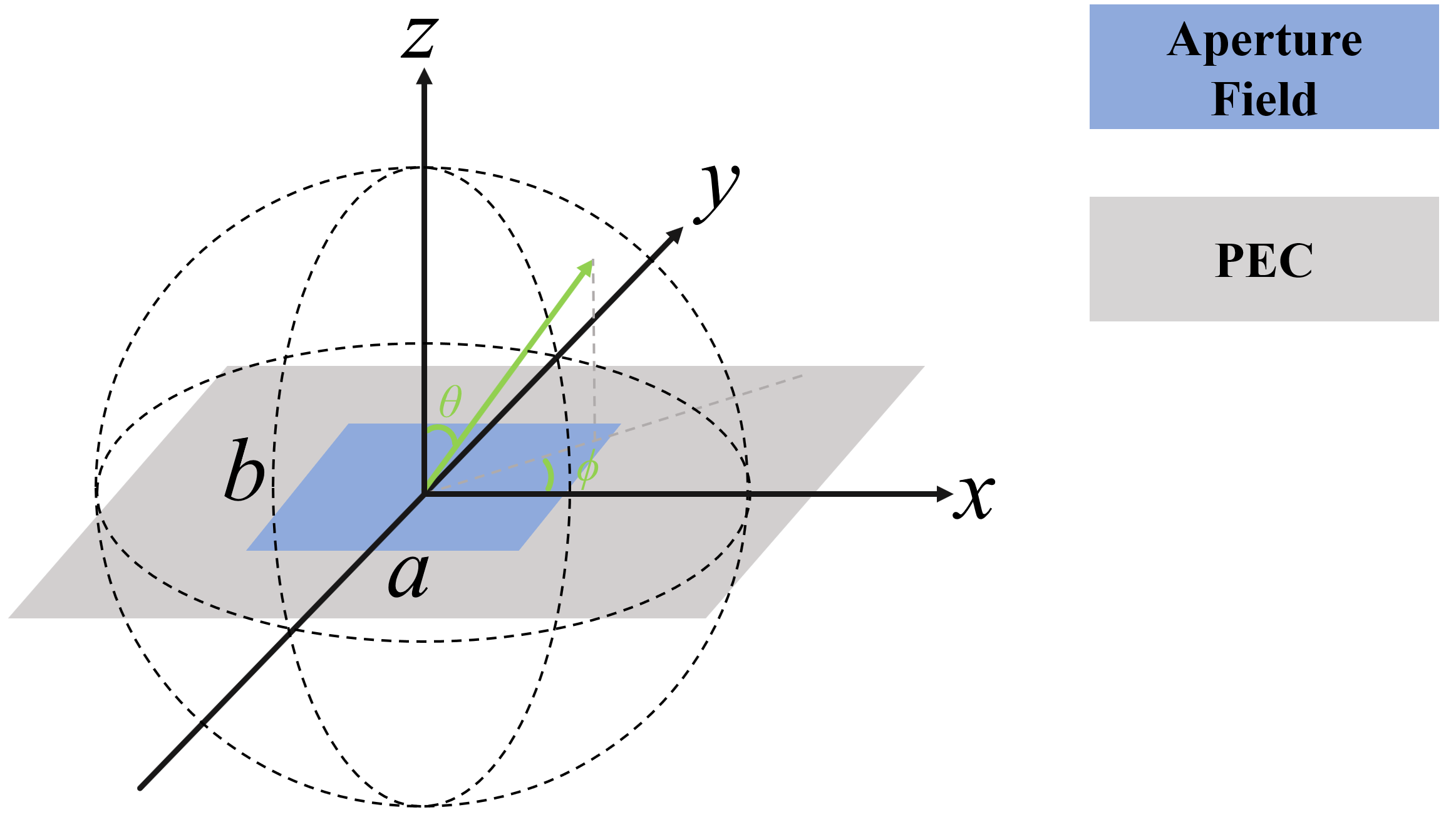
Figure 1: Schematic diagram of the general forward aperture problem

In the spectral domain, as written in (1), the monochromatic wave field $\boldsymbol{E}(x,y,z)$ radiated by the aperture field can be regarded as a superposition of plane waves of the form $\boldsymbol{f}\left(\theta,\phi\right)\exp({-j\boldsymbol{k}\cdot\boldsymbol{r}})$[25].

$$\boldsymbol{E}(x,y,z)=\frac{1}{4\pi^{2}}\int_{-\infty}^{\infty}{\int_{-\infty}^{\infty}{\boldsymbol{f}\left(\theta,\phi\right)e^{-j\boldsymbol{k}\cdot\boldsymbol{r}}}}\mathrm{d}k_{x}\mathrm{d}k_{y}$$ (1)

where $k_{x}=k\sin\theta\cos\phi$, $k_{y}=k\sin\theta\sin\phi$, and $k_{z}^{2}=k^{2}-k_{x}^{2}-k_{y}^{2}$. $\boldsymbol{f}$ consists of $f_{x}$ and $f_{y}$ given by (2).

$$f_{x}(\theta,\phi) =\int_{-\frac{b}{2}}^{\frac{b}{2}}\int_{-\frac{a}{2}}^{\frac{a}{2}}E_{\mathrm{ape},x}(x^{\prime},y^{\prime})\cdot e^{j(k_{x}x^{\prime}+k_{y}y^{\prime})}\mathrm{d}x^{\prime}\mathrm{d}y^{\prime}$$ (2a)

$$f_{y}(\theta,\phi) =\int_{-\frac{b}{2}}^{\frac{b}{2}}\int_{-\frac{a}{2}}^{\frac{a}{2}}E_{\mathrm{ape},y}(x^{\prime},y^{\prime})\cdot e^{j(k_{x}x^{\prime}+k_{y}y^{\prime})}\mathrm{d}x^{\prime}\mathrm{d}y^{\prime}$$ (2b)

The far-field asymptotic evaluation of (1) is given by (3), by using the Stationary Phase method[26].

$$\boldsymbol{E}(r,\theta,\phi)\approx\ j\frac{ke^{-jkr}}{2\pi r}\boldsymbol{e}_{\mathrm{far}}(\theta,\phi)$$ (3a)

$$\boldsymbol{e}_{\mathrm{far}}(\theta,\phi) =\boldsymbol{\hat{a}}_{\theta}e_{\mathrm{far},\theta}(\theta,\phi)+\boldsymbol{\hat{a}}_{\phi}e_{\mathrm{far},\phi}(\theta,\phi)$$ (3b)

$$=\boldsymbol{\hat{a}}_{\theta}\left(f_{x}\cos\phi+f_{y}\sin\phi\right)$$

$$\quad+\boldsymbol{\hat{a}}_{\phi}[\cos\theta\left(-f_{x}\sin\phi+f_{y}\cos\phi\right)]$$

In most cases, we pay more attention to the pattern $\boldsymbol{e}_{\mathrm{far}}(\theta,\phi)$ than the coefficient on distance $j\frac{ke^{-jkr}}{2\pi r}$. Obviously, $\boldsymbol{e}_{\mathrm{far}}$ here includes both polarization and phase information.

III Inverse Design Method

This section introduces the formulation of the inverse design method. Specifically, IDMBSA can be summarized into two steps. The first step is getting $|f_{x}|$ and $|f_{y}|$ from the desired $|e_{\mathrm{far},\theta}|$ and $|e_{\mathrm{far},\phi}|$. Additionally, for practical engineering applications, we also provide formulas to extract $|f_{x}|$ and $|f_{y}|$ from other polarization decompositions, such as horizontal (H) $|e_{\mathrm{far},h}|$ and vertical (V) polarization $|e_{\mathrm{far},v}|$. The second step is finding a suitable set of solutions ($E_{\mathrm{ape},x}$ and $E_{\mathrm{ape},y}$) from $|f_{x}|$ and $|f_{y}|$.

III-A Dealing with Phaseless Radiation Pattern

This subsection focuses on how to introduce phaseless patterns into the existing formulations, so as to convert phaseless pattern targets into constraints on aperture field. From (3b) we can derive (4), through algebraic transformations.

$$f_{x}(\theta,\phi) =e_{\mathrm{far},\theta}(\theta,\phi)\cos\theta-e_{\mathrm{far},\phi}(\theta,\phi){\sin\phi}/{\cos\theta}$$ (4a)

$$f_{y}(\theta,\phi) =e_{\mathrm{far},\theta}(\theta,\phi)\sin\phi+e_{\mathrm{far},\phi}(\theta,\phi){\cos\phi}/{\cos\theta}$$ (4b)

During the inverse design process, what usually given is $\left|e_{\mathrm{far},\theta}\right|$ and $\left|e_{\mathrm{far},\phi}\right|$ (the absolute value symbol here represents phaseless). Since $\left|e_{\mathrm{far},\theta}\right|$ and $\left|e_{\mathrm{far},\phi}\right|$ cannot be directly substituted into (4), we take the modulus of both sides of (4) and obtain (5). $\gamma$ in (5) is a function of $\theta$ and $\phi$, which represents the phase difference of two polarization components at a certain direction $(\theta,\phi)$.

$$\begin{split}\left|f_{x}(\theta,\phi)\right|=\bigg{(}&\left|e_{\mathrm{far},\theta}\right|^{2}\left|\cos\theta\right|^{2}+\left|e_{\mathrm{far},\phi}\frac{\sin\phi}{\cos\theta}\right|^{2}\\ &\qquad-2\left|e_{\mathrm{far},\theta}\right|\left|e_{\mathrm{far},\phi}\right|\left|\sin\phi\right|\cos\gamma\bigg{)}^{\frac{1}{2}}\end{split}$$ (5a)

$$\begin{split}\left|f_{y}(\theta,\phi)\right|=\bigg{(}&\left|e_{\mathrm{far},\theta}\right|^{2}\left|\sin\phi\right|^{2}+\left|e_{\mathrm{far},\phi}\right|^{2}\left|\frac{\cos\phi}{\cos\theta}\right|^{2}\\ &\qquad+2\left|e_{\mathrm{far},\theta}\right|\left|e_{\mathrm{far},\phi}\right|\left|\frac{\sin\phi\cos\phi}{\cos\theta}\right|\cos\gamma\bigg{)}^{\frac{1}{2}}\end{split}$$ (5b)

Combined with engineering applications, we also give another expression of (5) for horizontal (H) and vertical (V) polarization ($|e_{\mathrm{far},h}|$ and $|e_{\mathrm{far},v}|$), by using the Ludwig3 coordinate system, as shown in (6).

$$|f_{x}(\theta,\phi)|=\sqrt{|l_{1}|^{2}+|l_{2}|^{2}+2|l_{1}||l_{2}|\cos\gamma}$$ (6a)

$$|f_{y}(\theta,\phi)|=\sqrt{|l_{3}|^{2}+|l_{4}|^{2}+2|l_{3}||l_{4}|\cos\gamma}$$ (6b)

where

$$l_{1} =e_{\mathrm{far},h}\left(\cos^{2}\phi+\sin^{2}\phi/\cos\theta\right);$$

$$l_{2} =e_{\mathrm{far},v}\sin\phi\cos\phi\left(1-1/\cos\theta\right);$$

$$l_{3} =e_{\mathrm{far},h}\sin\phi\cos\phi\left(1-1/\cos\theta\right);$$

$$l_{4} =e_{\mathrm{far},v}\left(\sin^{2}\phi+\cos^{2}\phi/\cos\theta\right);$$

Several common cases regarding (6) are discussed next.

• Case I: Linear Polarization

  When only a single polarization is needed, another orthogonal polarization can be set to 0. For example, when only the V polarization $e_{\mathrm{far},v}$ is considered, (6) degenerates to (7).

$$|f_{x}(\theta,\phi)|=|l_{2}|;\ |f_{y}(\theta,\phi)|=|l_{4}|$$ (7)

• Case II: Circular Polarization

  Circular polarization requires that the modulus values of the two polarization components are equal, and the phase difference is $90^{\circ}$. That is $|e_{\mathrm{far},h}|=|e_{\mathrm{far},v}|$, and $\gamma=90^{\circ}$ in any direction $(\theta,\phi)$. Then, (6) degenerates to (8).

$$|f_{x}(\theta,\phi)|=\sqrt{|l_{1}|^{2}+|l_{2}|^{2}};\ |f_{y}(\theta,\phi)|=\sqrt{|l_{3}|^{2}+|l_{4}|^{2}}$$ (8)

• Case III: Elliptical Polarization

  Once $\gamma$ is determined, (6) itself corresponds to elliptical polarization.

The $|f_{x}|$ and $|f_{y}|$ in (5) and (6) act as bridges to deliver the phaseless pattern constraints to the aperture field constraints.

Obviously, it is easy to get $|f_{x}|$ and $|f_{y}|$ from the desired $|e_{\mathrm{far},\theta}|$ and $|e_{\mathrm{far},\phi}|$ or $|e_{\mathrm{far},h}|$ and $|e_{\mathrm{far},v}|$ by using (5) or (6).

III-B Solving Integral Equation for Aperture Field

Next, what we need is to find a suitable set of solutions ($E_{\mathrm{ape},x}$ and $E_{\mathrm{ape},y}$) from $|f_{x}|$ and $|f_{y}|$ according to (9).

$$|f_{x}(\theta,\phi)| =\left|\int_{-\frac{b}{2}}^{\frac{b}{2}}\int_{-\frac{a}{2}}^{\frac{a}{2}}E_{\mathrm{ape},x}(x^{\prime},y^{\prime})\cdot e^{j(k_{x}x^{\prime}+k_{y}y^{\prime})}\mathrm{d}x^{\prime}\mathrm{d}y^{\prime}\right|$$ (9a)

$$|f_{y}(\theta,\phi)| =\left|\int_{-\frac{b}{2}}^{\frac{b}{2}}\int_{-\frac{a}{2}}^{\frac{a}{2}}E_{\mathrm{ape},y}(x^{\prime},y^{\prime})\cdot e^{j(k_{x}x^{\prime}+k_{y}y^{\prime})}\mathrm{d}x^{\prime}\mathrm{d}y^{\prime}\right|$$ (9b)

During this step, the inverse Fourier transform cannot be applied in (9), because the addition of the absolute value symbol on the right-hand side eliminates all phase information. The root cause is the non-linearity introduced by the phaseless. (In mathematics, taking the modulus value on both sides of (2) is (9)). Therefore, we can only treat (9) as the first kind of two-dimensional Fredholm integral equations after the modulo operation, which is difficult to obtain analytical solutions[27]. Here, we will employ modal expansion and MOO to approximately solve (9).

III-B1 Modal Expansion on Aperture Field

First, expand the unknown integrand $\boldsymbol{E}_{\mathrm{ape}}$ using the modal expansion method. The physical constraints can be cleverly introduced into the integral equation with the help of boundary conditions. As can be seen from Fig. 1, $\boldsymbol{E}_{\mathrm{ape}}$ satisfies (10). The modal expansion of $\boldsymbol{E}_{\mathrm{ape}}$ is expressed by the terms in the braces of (11), and it follows easily that $\boldsymbol{E}_{\mathrm{ape}}$ can be approximated by a finite number of unknown modal coefficients and known modal terms.

$$\left\{\begin{array}[]{l}E_{\mathrm{ape},x}|_{y=-\frac{b}{2},\frac{b}{2}}=0\\ E_{\mathrm{ape},y}|_{x=-\frac{a}{2},\frac{a}{2}}=0\\ \end{array}\right.$$ (10)

Equation (11) converts the problem of solving $\boldsymbol{E}_{\mathrm{ape}}(x,y)$ to solving the unknown complex modal coefficients $\alpha_{mn}^{i}$ and $\beta_{mn}^{i}$, $(i=x,y)$. The selection of the basis function is not unique. The trigonometric functions were chosen because they are the harmonic functions of the waveguide harmonic equation, if we regard the modal shown in Fig. 1 as a waveguide connected to the infinite PEC plane. The analytical integration of (11) is provided in Appendix A. Thanks to the availability of an analytical expression, (11) can be integrated analytically instead of numerically, resulting in a significant improvement in computational efficiency. The number of optimization variables in general array synthesis methods is proportional to the aperture area. For example, for an array with area $L^{2}$ [$\lambda^{2}$], the number of ports is about $(L/0.5)^{2}=4L^{2}$, if the spacing of elements is $0.5[\lambda]$. The variable to be optimized is about $8L^{2}$ (considering amplitude and phase). Whereas, in IDMBSA, the number of optimization variables is associated with the number of modes and increases slowly with the expansion of the aperture area. The determination of the number of modes in IDMBSA is elaborated in Section IV-B. A rough comparison graph is summarized in Fig. 2.

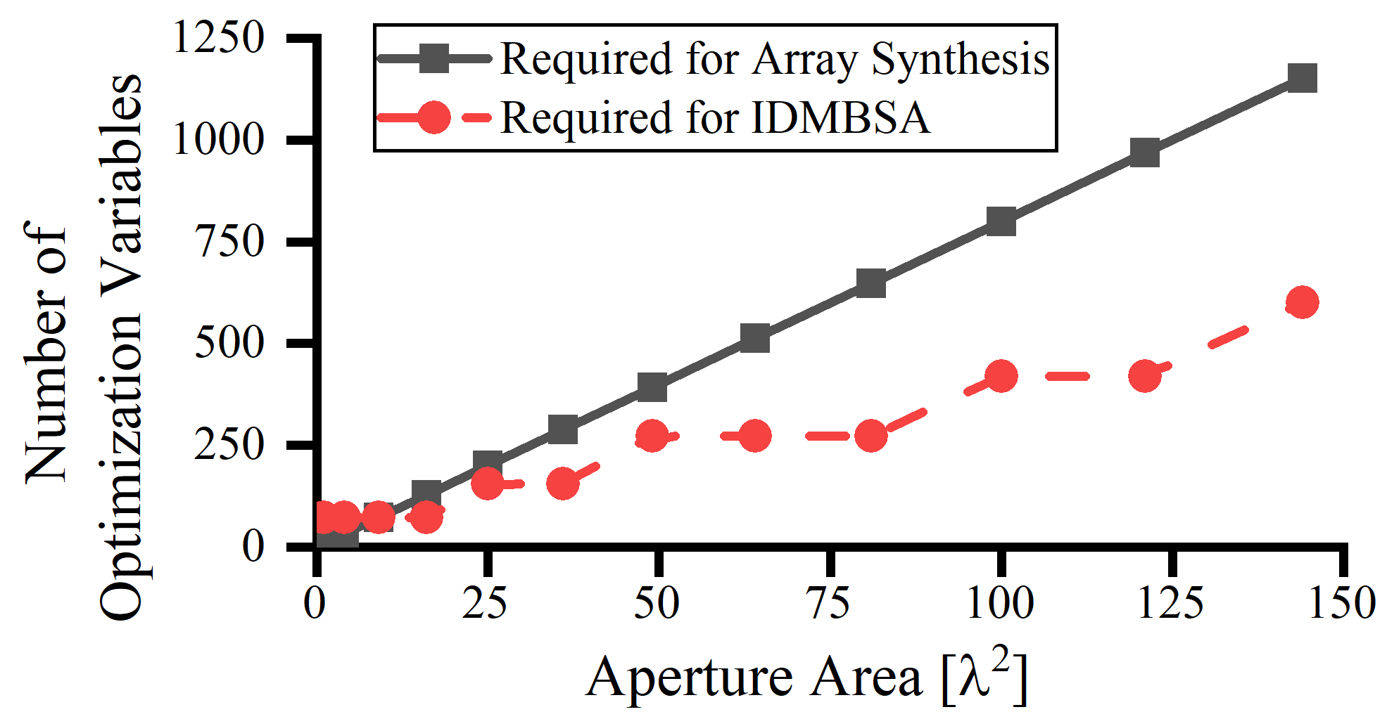
Figure 2: Variation of the number of optimization variables with aperture area

III-B2 Obtain Modal Coefficients by Using MOO

We obtain $\alpha_{mn}^{i}$ and $\beta_{mn}^{i}$ $(i=x,y)$ by using the PSO toolbox (uploaded to [28]), and define (12) as the cost function. The parameter settings for PSO are as follows: the population size is set to 40, with a maximum iteration limit of 100. The initial inertia weight is 0.9, gradually decreasing to 0.4 as the number of iterations increases. The cognitive and social learning factors are set to 0.5 and 1.25. The initial positions and velocities of the population are randomly generated in the solution space.

The selection of MOO is not exclusive. This study employed PSO due to its exceptional multi-variable problem adaptability and the author’s familiarity with PSO. Other MOOs, such as GA [17], are equally suitable alternatives. In fact, directly using the ’interior-point’ default optimization method built into the MATLAB fmincon function can also achieve optimization (unfortunately, this method is time-consuming and not recommended).

The choice of cost function is not unique and can be selected according to the design requirements. Here, we use the Pearson’s distance between $|\boldsymbol{f}_{\mathrm{tar}}(\theta,\phi)|$ and $|\boldsymbol{f}_{\mathrm{cal}}(\theta,\phi)|$ as the cost function.

$$obj=1-\rho_{X,Y}=1-\frac{\sum_{i=1}^{n}\left(x_{i}-\bar{x}\right)\left(y_{i}-\bar{y}\right)}{\sqrt{\sum_{i=1}^{n}\left(x_{i}-\bar{x}\right)^{2}\sum_{i=1}^{n}\left(y_{i}-\bar{y}\right)^{2}}}$$ (12)

where $X=|\boldsymbol{f}_{\mathrm{tar}}(\theta,\phi)|$ and $Y=|\boldsymbol{f}_{\mathrm{cal}}(\theta,\phi)|$. $x_{i}$ represents an element in $X$, and $\bar{x}$ denotes the average of all elements in $X$, similarly, $y_{i}$ and $\bar{y}$ follow the same logic. $|\boldsymbol{f}_{\mathrm{tar}}|$ is known from (5) and (6), and $\boldsymbol{f}_{\mathrm{cal}}$ is calculated from the optimized $\alpha_{mn}^{y}$ and $\beta_{mn}^{y}$.

$$\left|f_{x}(\theta,\phi)\right|=\Bigg{|}\int_{-\frac{b}{2}}^{\frac{b}{2}}{\int_{-\frac{a}{2}}^{\frac{a}{2}}{}} \left\{\sum_{n=1}^{N}\left[\left(\sum_{m=1}^{M}\alpha_{mn}^{x}\sin\left(\frac{m\pi}{a}(x^{\prime}+\frac{a}{2})\right)+\sum_{m=0}^{M}\beta_{mn}^{x}\cos\left(\frac{m\pi}{a}(x^{\prime}+\frac{a}{2})\right)\right)\sin\left(\frac{n\pi}{b}(y^{\prime}+\frac{b}{2})\right)\right]\right\}$$ (11a)

$$e^{j(k_{x}x^{\prime}+k_{y}y^{\prime})}\mathrm{d}x^{\prime}\mathrm{d}y^{\prime}\Bigg{|}$$

$$|f_{y}(\theta,\phi)|=\Bigg{|}\int_{-\frac{b}{2}}^{\frac{b}{2}}{\int_{-\frac{a}{2}}^{\frac{a}{2}}{}} \left\{\sum_{m=1}^{M}\left[\left(\sum_{n=1}^{N}\alpha_{mn}^{y}\sin\left(\frac{n\pi}{b}(y^{\prime}+\frac{b}{2})\right)+\sum_{n=0}^{N}\beta_{mn}^{y}\cos\left(\frac{n\pi}{b}(y^{\prime}+\frac{b}{2})\right)\right)\sin\left(\frac{m\pi}{a}(x^{\prime}+\frac{a}{2})\right)\right]\right\}$$ (11b)

$$e^{j(k_{x}x^{\prime}+k_{y}y^{\prime})}\mathrm{d}x^{\prime}\mathrm{d}y^{\prime}\Bigg{|}$$

III-C The IDMBSA Process: A Step-by-Step Guide

According to (5)-(12), IDMBSA can be employed for determining the aperture field for arbitrary phaseless far-field.

The detailed inverse design process is performed as follows:

Step A: Calculate $|f_{x}|$ and $|f_{y}|$ using (5) or (6) based on the target phaseless far-field radiation pattern. If the far-field polarization requirements are specific, coordinate transformation can be referred to (see [24]).

Step B: Determine certain technical parameters in (11), such as the number of sampling points for $\theta$ and $\phi$. For the formulations set up in this paper, it is recommended that M and N take values up to $2a/\lambda$ and $2b/\lambda$, as detailed in Section IV-B.

Step C: Solve for the unknown coefficients $\alpha_{mn}^{i}$ and $\beta_{mn}^{i}$ in (11) using MOO algorithms. The choice of optimization algorithm and cost function are not unique; we have achieved good results using PSO and (12).

IV Numerical Simulation

This section shows numerical experiments using IDMBSA to obtain aperture field that can produce specific $|\boldsymbol{e}_{\mathrm{tar}}|$.

IV-A Design Targets

Here, we employ array factors to generate a set of design targets. Consider a 16$\times$16 broadside array located in the $xoy$ plane with uniform amplitude excitation, where the spacing between elements is $\lambda/{2}$. By directly rotating the coordinate system, we can obtain a set of target patterns with different beam direction angles but the same directivity of 25.2 dBi and side lobe level (SLL) of -13.5 dB. Here, we present two cases, $(30^{\circ},0^{\circ})$ and $(60^{\circ},0^{\circ})$, and plot their normalized patterns as shown in Fig. 3.

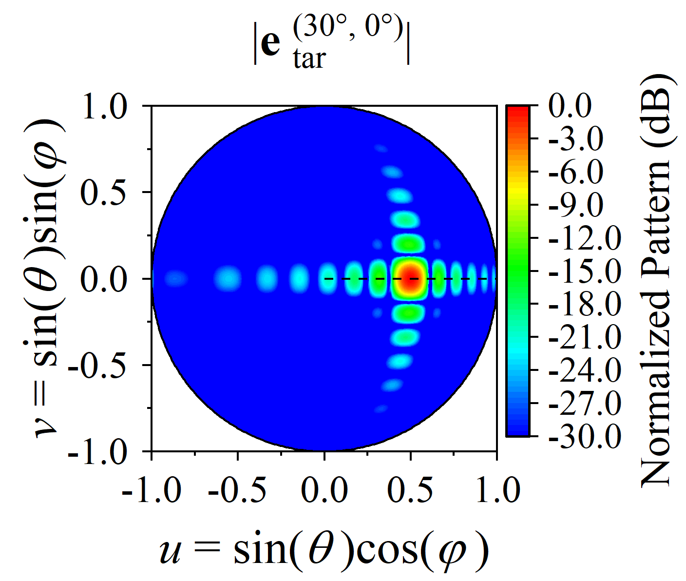
(a)

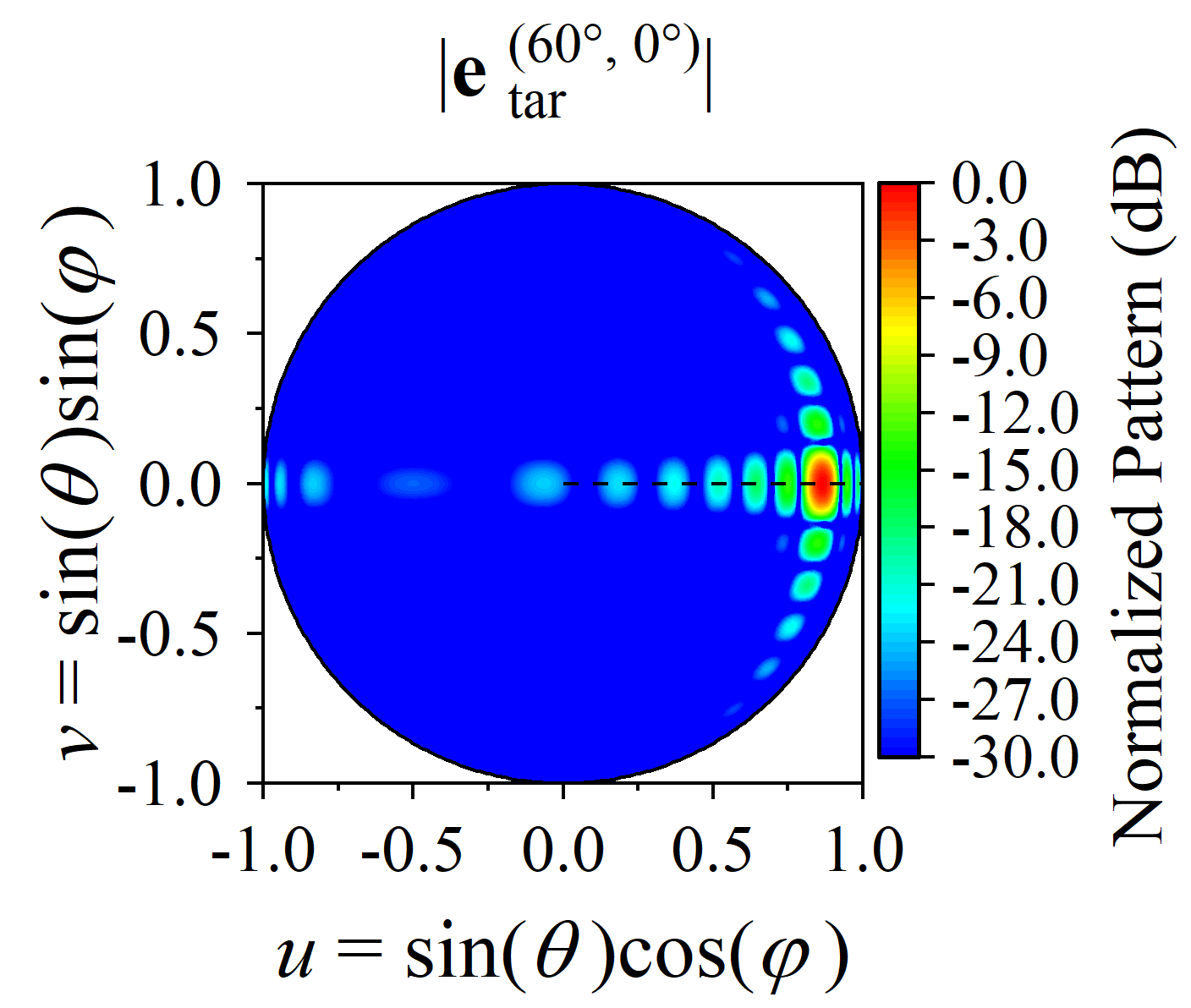
(b)

Figure 3: Target normalized radiation patterns. (a) $|\boldsymbol{e}_{\mathrm{tar}}^{(30^{\circ},0^{\circ})}|$; (b) $|\boldsymbol{e}_{\mathrm{tar}}^{(60^{\circ},0^{\circ})}|$.

Assume that the polarization is only V polarization, represented by (13), as mentioned in case I of section III. This assumption is not absolute, IDMBSA applies to any polarization distribution. In the following section, we also present a case study on independent design for dual polarization in Section V-C.

$$|{e}_{\mathrm{tar},v}^{\text{scan\_angle}}| =|\boldsymbol{e}_{\mathrm{tar}}^{\text{scan\_angle}}|$$ (13a)

$${e}_{\mathrm{tar},h}^{\text{scan\_angle}} =0$$ (13b)

Once targets are determined, the first step is to calculate $|f_{x}|$ and $|f_{y}|$ by using (7). Here, we only consider $|f_{y}|$, because the calculated $|f_{x}|$ is approximately 0. Thus, the aperture field has only $E_{\mathrm{ape},y}^{\text{scan\_angle}}$, but no $E_{\mathrm{ape},x}^{\text{scan\_angle}}$.

IV-B Numerical Simulation Settings

In the following numerical simulations, the partitioning method for $\theta$ and $\phi$ is not absolute and can be adjusted based on the oscillation of the target pattern. Here, $\theta$ from 0 to $\pi/2$ and $\phi$ from 0 to $2\pi$ are divided into 45 and 180 parts, respectively.

The aperture size $a$ and $b$ are set to $7.5\lambda$, as the same area as the 16$\times$16 array. Regarding the values of M and N, fewer modes limit design freedom, at times hindering target attainment. Excessive modes raise computational load, casusing the field vary dramatically and difficult to achieve. It is worth noting that when applying IDMBSA to array synthesis, the upper limit of theoretically achievable distortion-free modes in the array can be determined according to the Nyquist-Shannon theorem. Based on this, the upper limits for M and N should be $a/d_{x}$ and $b/d_{y}$, respectively. ( $d_{x}$ and $d_{y}$ represent the spacing between array elements.) In this paper, M and N are set to 8, while for the $(60^{\circ},0^{\circ})$ case they are set to 12.

The next step is solving $E_{\mathrm{ape},y}^{\text{scan\_angle}}$ (more precisely, obtaining $\alpha_{mn}^{y}$ and $\beta_{mn}^{y}$) from $|f_{y}|$ according to (11b) by PSO. In the iterative optimization process, the integration in (11b) is accelerated by using its analytical solution (15b).

IV-C Numerical Simulation Results

The normalized amplitude and phase distribution of $E_{\mathrm{ape},y}^{(30^{\circ},0^{\circ})}$ and $E_{\mathrm{ape},y}^{(60^{\circ},0^{\circ})}$ calculated by IDMBSA are shown in Fig. 4. We performed full-wave simulations using CST Microwave Studio to verify the correctness. First, constructed $E_{\mathrm{ape},y}$ shown in Fig. 4 by using scripts to modify files with the extensions “nfs” and “xml” from CST. The modified source files were excited in CST, and normalized radiation patterns of $E_{\mathrm{ape},y}^{(30^{\circ},0^{\circ})}$ and $E_{\mathrm{ape},y}^{(60^{\circ},0^{\circ})}$ are shown in Fig. 5(a, b), with their directivity are 24.2 dBi and 23.9 dBi, respectively. The boundary conditions are set as shown in Fig. 5(c). Additionally, their respective side lobe levels (SLL) are -13.9 dB and -11.5 dB. For better visualization, the 2D cut-plane at $v=0$ of the dashed lines in Fig. 5(b, c) are summarized in Fig. 5(d). The reviewer strongly believes that the number of modes chosen for the modal expansion could be a reason behind the mismatch. The relevant CST files with results have been uploaded to [28].

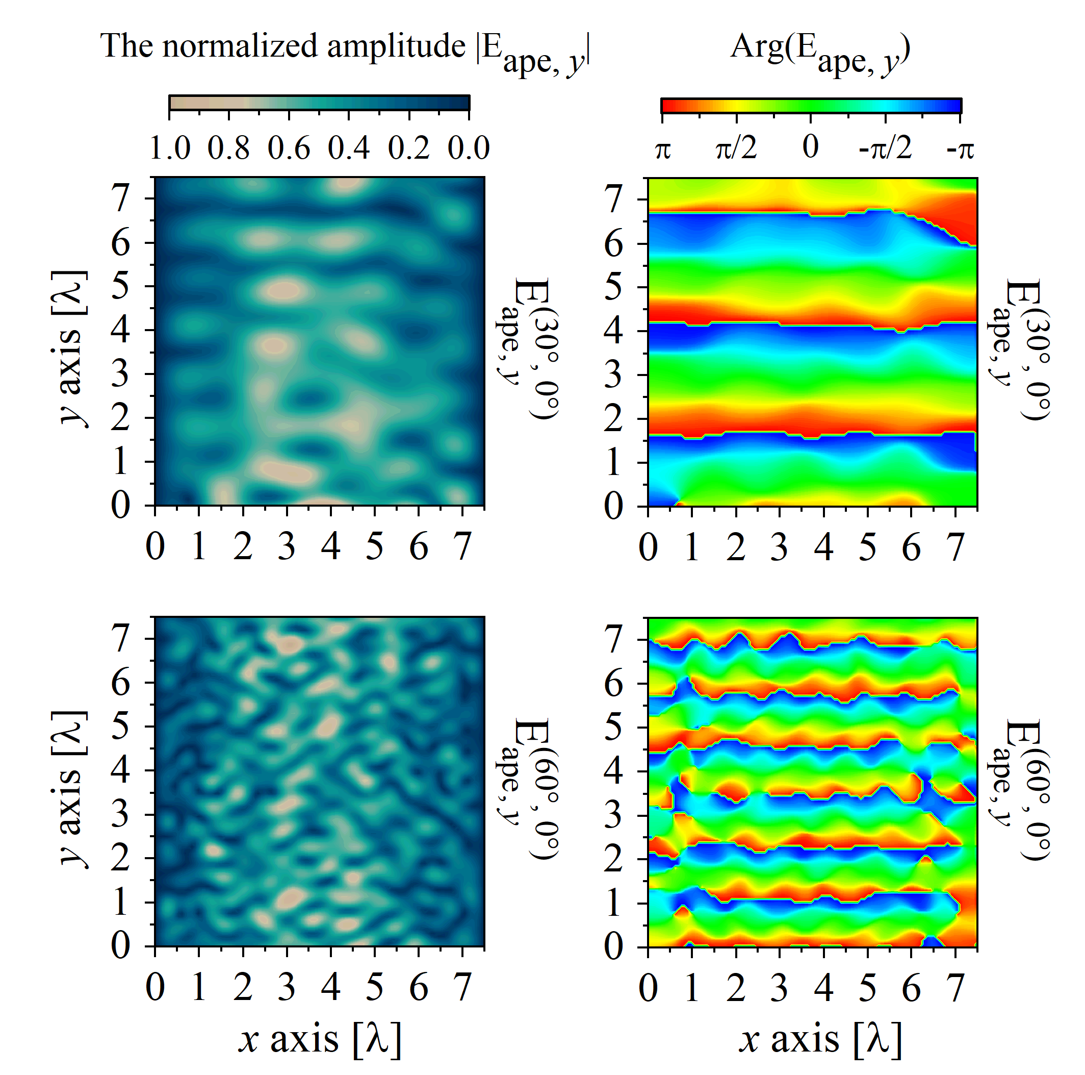
Figure 4: The normalized amplitude distribution and phase distribution of $E_{\mathrm{ape},y}^{(30^{\circ},0^{\circ})}$ and $E_{\mathrm{ape},y}^{(60^{\circ},0^{\circ})}$ .

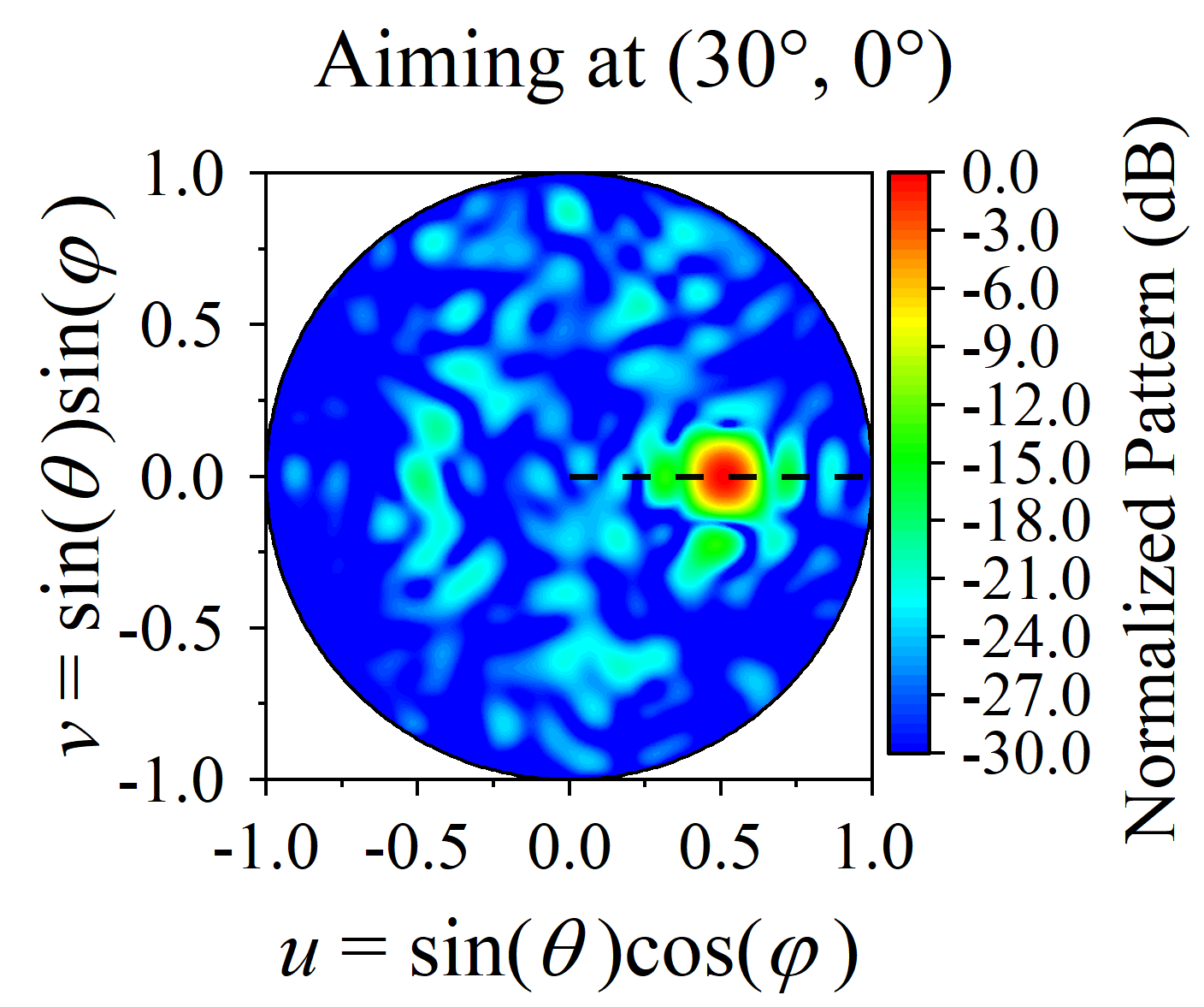
(a)

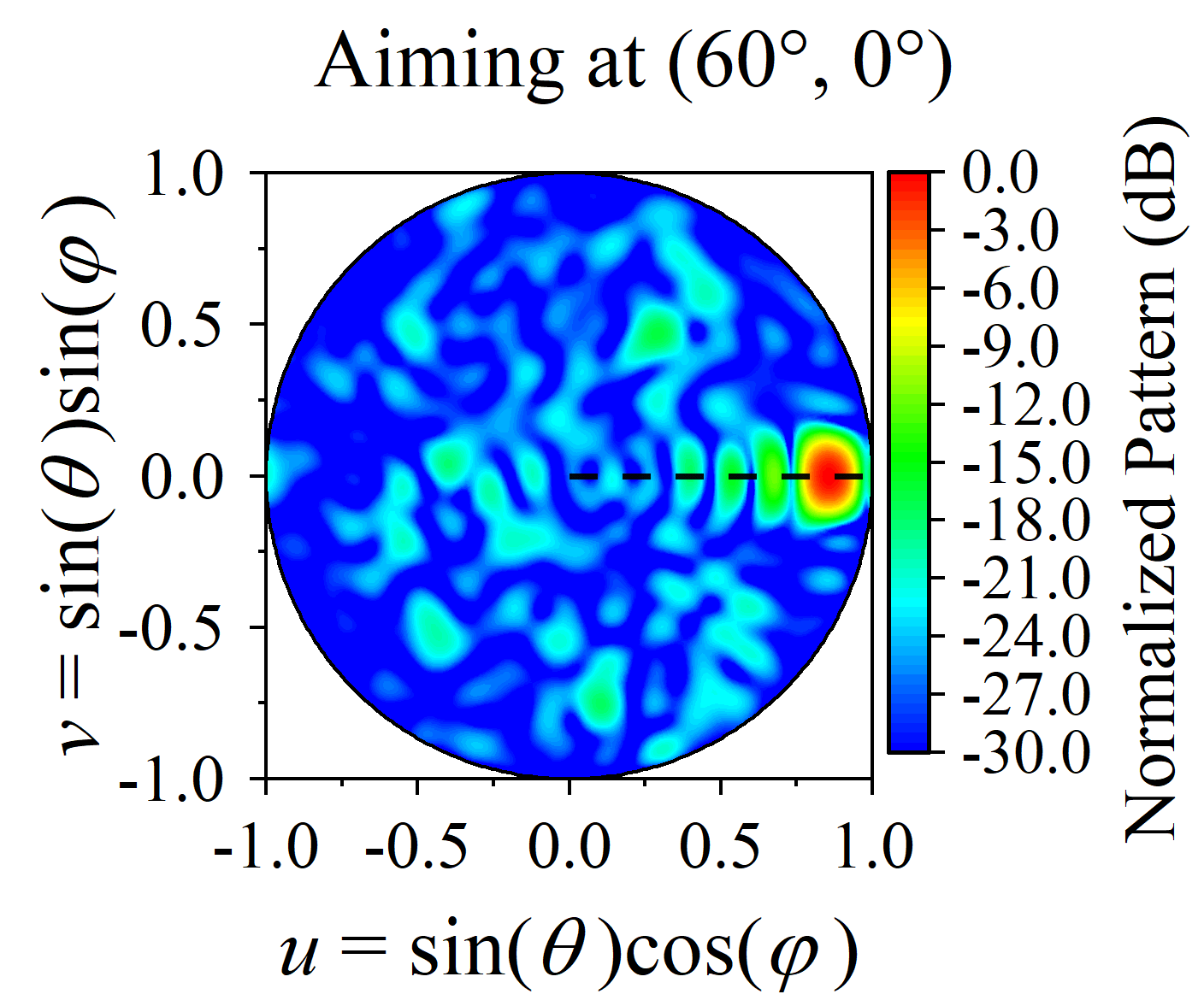
(b)

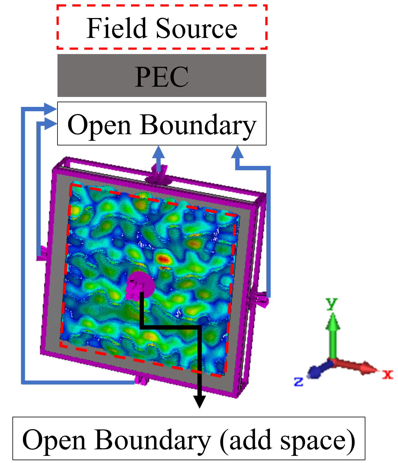
(c)

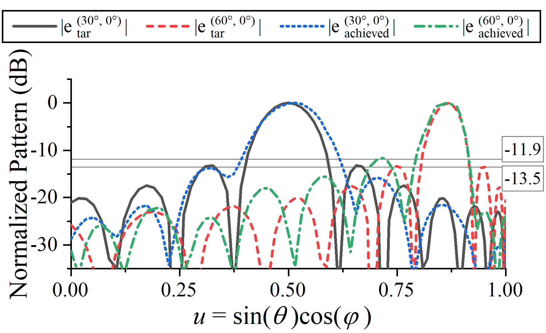
(d)

Figure 5: (a) Normalized radiation pattern of $E_{\mathrm{ape},y}^{(30^{\circ},0^{\circ})}$ ; (b) Normalized radiation pattern of $E_{\mathrm{ape},y}^{(60^{\circ},0^{\circ})}$; (c) Simulation settings in CST Microwave Studio; (d) 2D cut-plane: target vs. achieved.

V The application of IDMBSA

In the previous section, we successfully used IDMBSA to design a series of aperture field distributions for achieving specific radiation patterns. However, these aperture fields have not been physically implemented. In this section, we illustrate the physical implementation of the aperture fields through several case studies using microstrip antenna arrays, demonstrate the application of IDMBSA in existing array synthesis and antenna design. Most simulations have been uploaded to [28].

V-A Application of IDMBSA in Array Synthesis

In Section IV, the convention of (13) leaves the aperture field with only $E_{\mathrm{ape},y}^{\text{scan\_angle}}$. Therefore, a linearly polarized patch antenna is chosen as the array element, and the structure and S-parameters are depicted in Fig. 6. A planar array of 16$\times$16 elements is arranged, where the inter-element spacing is 61.18mm, half of the wavelength at 2.45GHz.

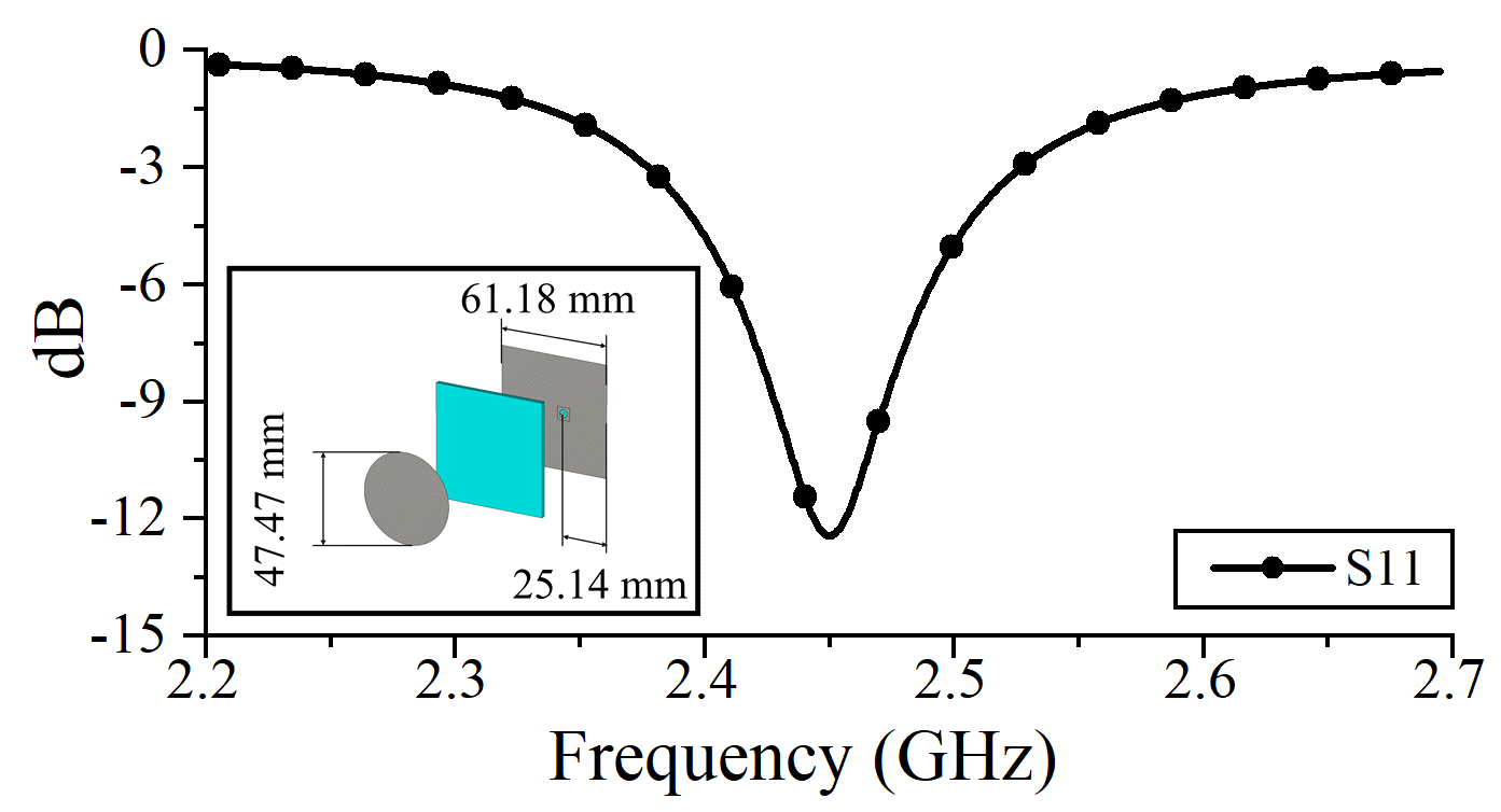
Figure 6: Array element and its S-parameter

The feeding amplitudes and phases of each element in the array are provided by the discretized $E_{\mathrm{ape},y}^{(30^{\circ},0^{\circ})}$. During the discretization process, we use complex electric field at the geometric center of each element as design basis, and the specific values are summarized in Fig. 7(a, b). The different polarization radiation patterns of the array are shown in Fig. 7(c,d), with a directivity of 23.4 dBi. The 2D cut-plane at $v=0$ of the dashed lines in Fig. 7(c) is summarized in Fig. 9(f). The simulation results are consistent with the expected pattern shown in Fig. 3(a), indicating that IDMBSA can be applied to array synthesis.

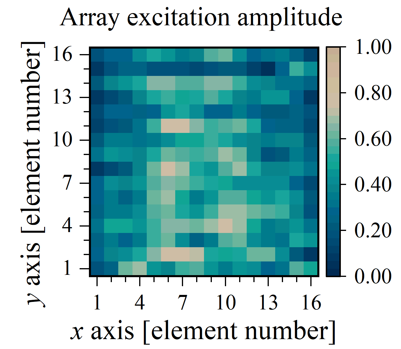
(a)

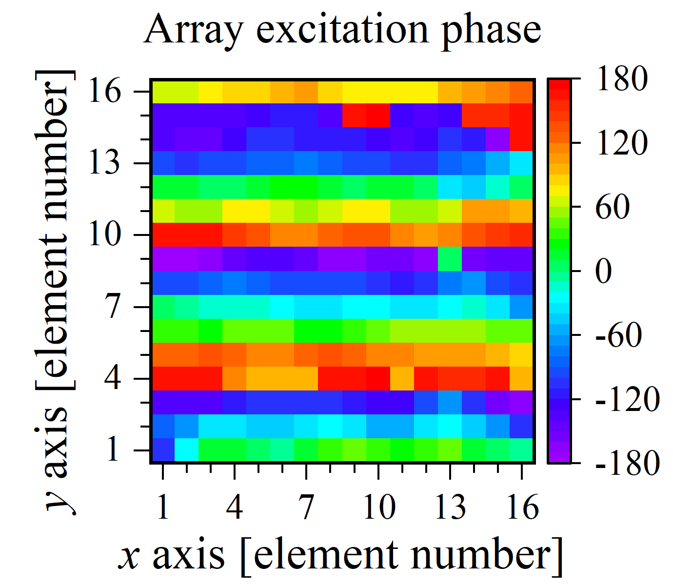
(b)

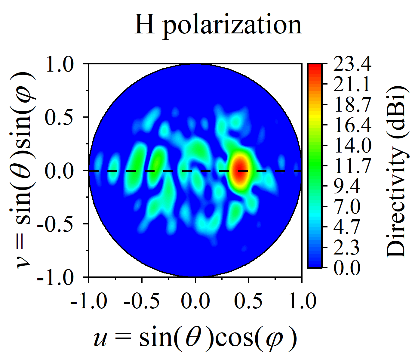
(c)

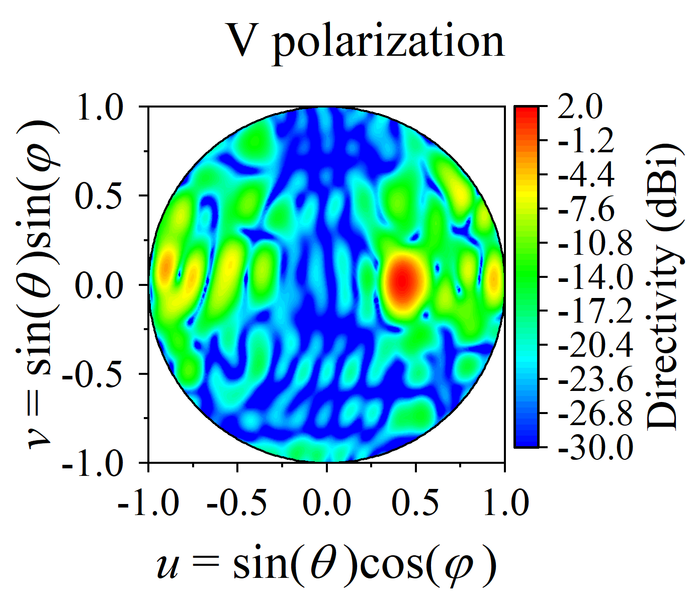
(d)

Figure 7: (a) Array excitation amplitude; (b) Array excitation phase; (c) Array radiation pattern (H polarization); (d) Array radiation pattern (V polarization).

V-B Application of IDMBSA in Sparse Array Design

Observing Fig. 7(a), it’s evident that many array elements have small normalized excitation, allowing us to designate them as dummy elements due to their negligible contributions in the far field. Based on numerical experiments, we find that when the total contribution of the low-radiating elements compared to the whole aperture is below 30%, sparse arrays can effectively replicate the desired performance. In this context, we’ve set the cutoff excitation amplitude at 0.5 (which means that elements with a normalized excitation amplitude less than 0.5 will not be excited), corresponding to the contribution of all low-radiating elements is 25.9%. The specific excitation setting is shown in Fig. 8(a). This approach yields similar radiation pattern. Furthermore, by removing the dummy elements, a new sparse array was constructed as shown in Fig. 8(b). It consists of 83 elements and its radiation patterns are shown in Fig. 8(c,d), with a directivity of 23.2 dBi. The 2D cut-plane at $v=0$ of the dashed lines in Fig. 8(c) is summarized in Fig. 9(f).

The above case demonstrates that IDMBSA can avoid the optimization of spatial coordinates with traditional sparse array design method[29, 30], and can be applied to sparse array design after post-processing (discretization and threshold-based selection).

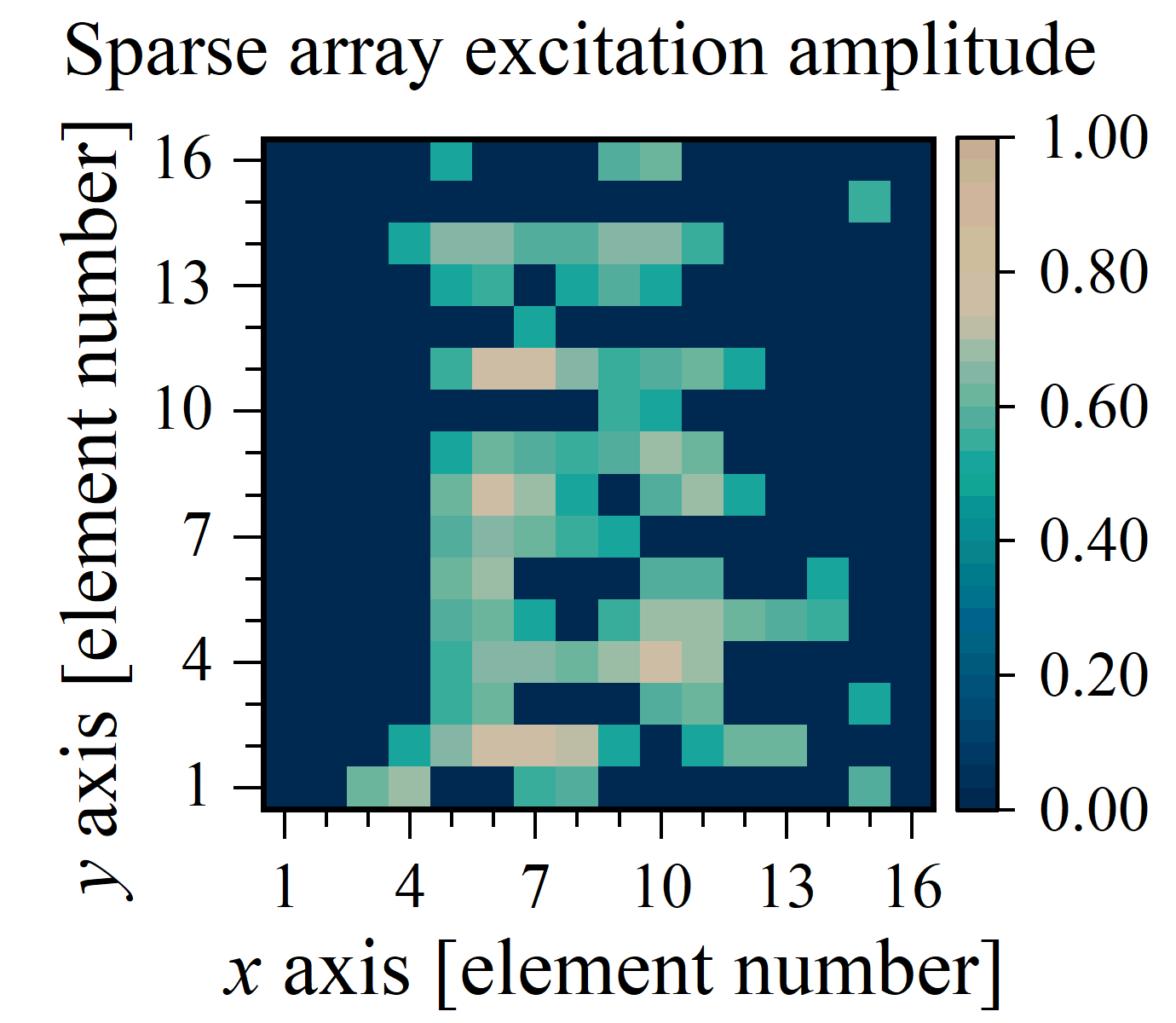
(a)

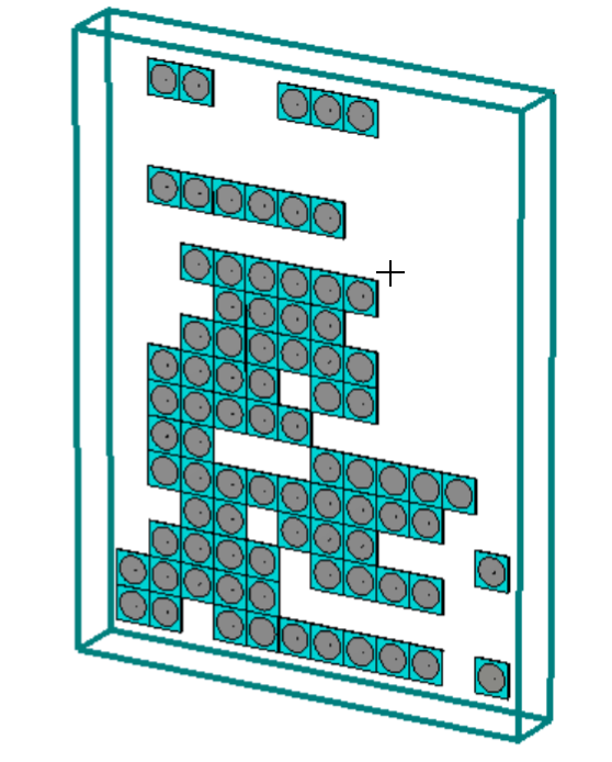
(b)

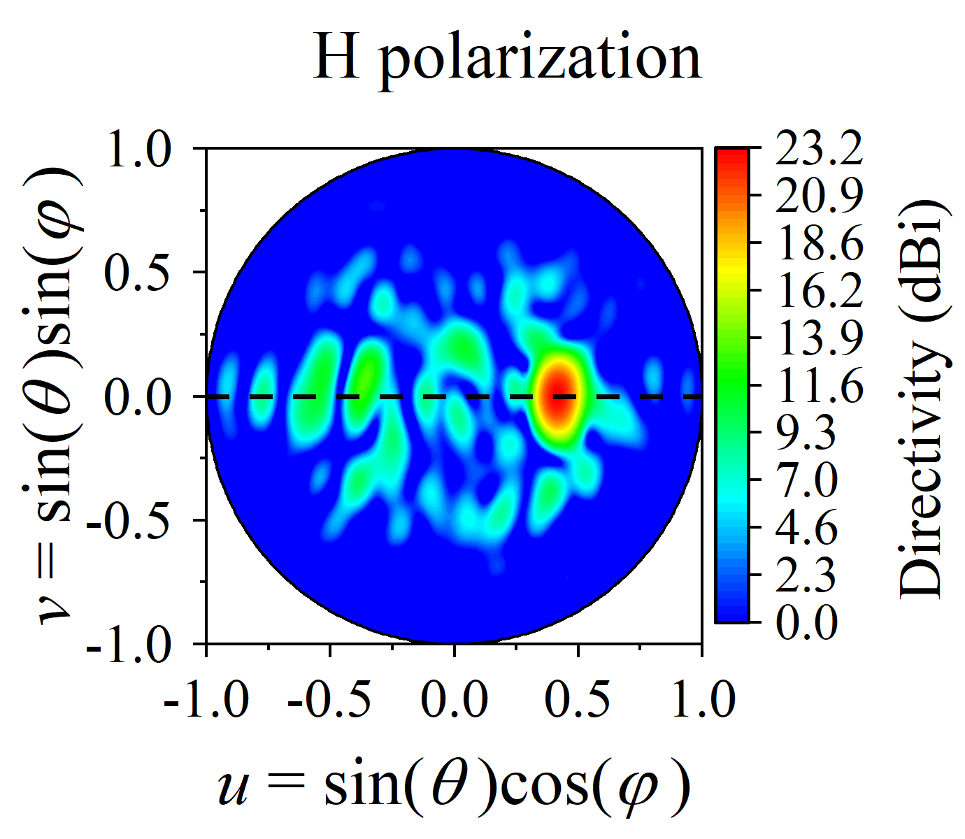
(c)

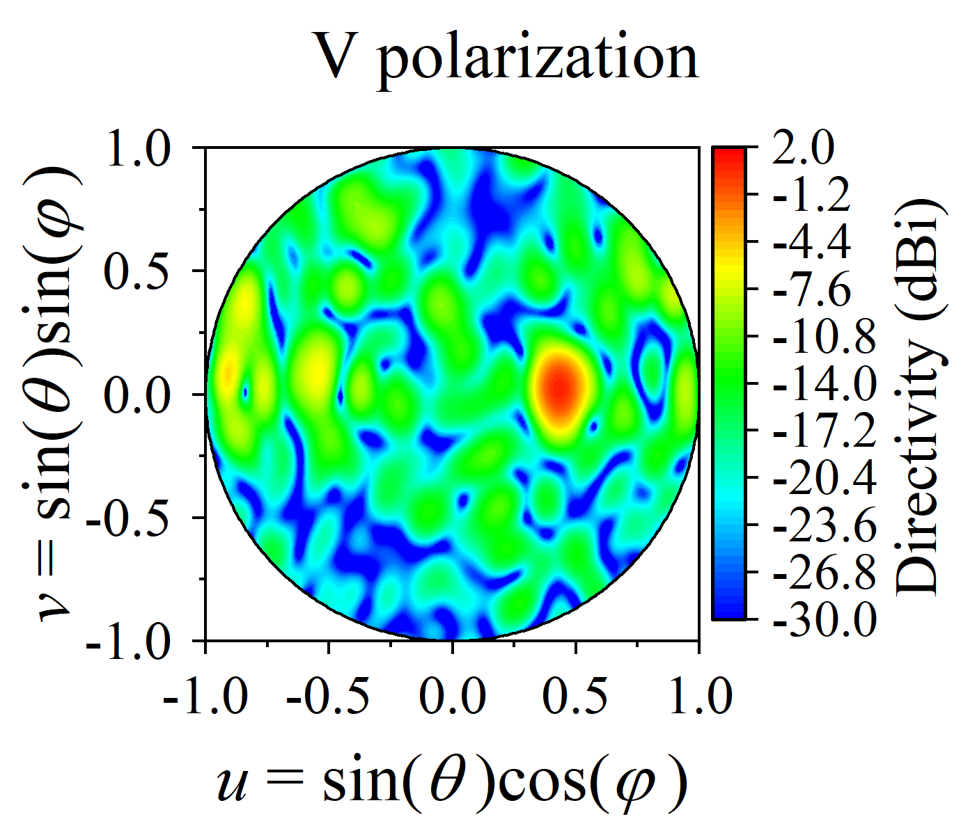
(d)

Figure 8: (a) Excitation amplitude of the sparse array; (b) Schematic diagram of the sparse array; (c) Radiation pattern of the sparse array (H polarization); (d) Radiation pattern of the sparse array (V polarization).

V-C Independent Design of Dual-Polarization using IDMBSA

This subsection presents a case of independently designing radiation patterns in both H and V polarization using IDMBSA. As we mentioned before, H polarization determines $E_{\mathrm{ape},x}$ and V polarization determines $E_{\mathrm{ape},y}$, so the two polarizations can be designed independently.

In this case, both H and V polarizations are configured to form single beams with different directional angles, as shown in (14).

$$|{e}_{\mathrm{design},v}| =|\boldsymbol{e}_{\mathrm{tar}}^{(30^{\circ},0^{\circ})}|$$ (14a)

$$|{e}_{\mathrm{design},h}| =|\boldsymbol{e}_{\mathrm{tar}}^{(0^{\circ},30^{\circ})}|$$ (14b)

The post-processed $E_{\mathrm{ape},y}^{(30^{\circ},0^{\circ})}$ field is consistent with Fig. 8(a), and the post-processed $E_{\mathrm{ape},x}^{(0^{\circ},30^{\circ})}$ field corresponds to a 90° rotation of Fig. 8(a). We verify this using both planar array and sparse array, and get similar results. For brevity, we present the results of the sparse array here. The array element is a modified patch antenna with dual-port feeding. The ports are adjusted to ensure the physical installation of SMA connectors, and its structure and S-parameters are shown in Fig. 9(a). The array is illustrated in Fig. 9(b). The array consists of 136 elements and 272 ports, but only 166 ports are utilized. Its radiation patterns are shown in Fig. 9(c,d,e). Additionally, their directivities are 20.4 dBi. The 2D cut-plane at $v=0$ of the dashed lines for both polarizations are summarized in Fig. 9(f). The observed mismatch in Fig. 9(f) between the results and the objectives on sidelobes and nulls may be attributed to an increased number of selected modes, thus hindering the accurate replication of the aperture field by the array.

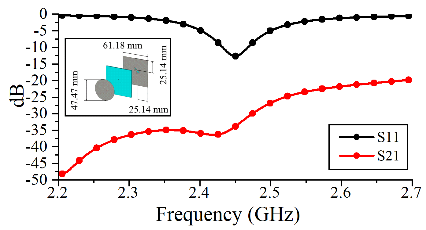
(a)

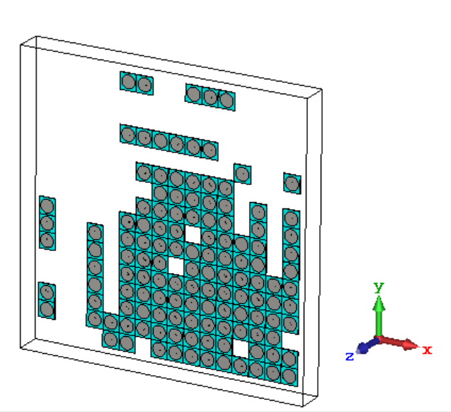
(b)

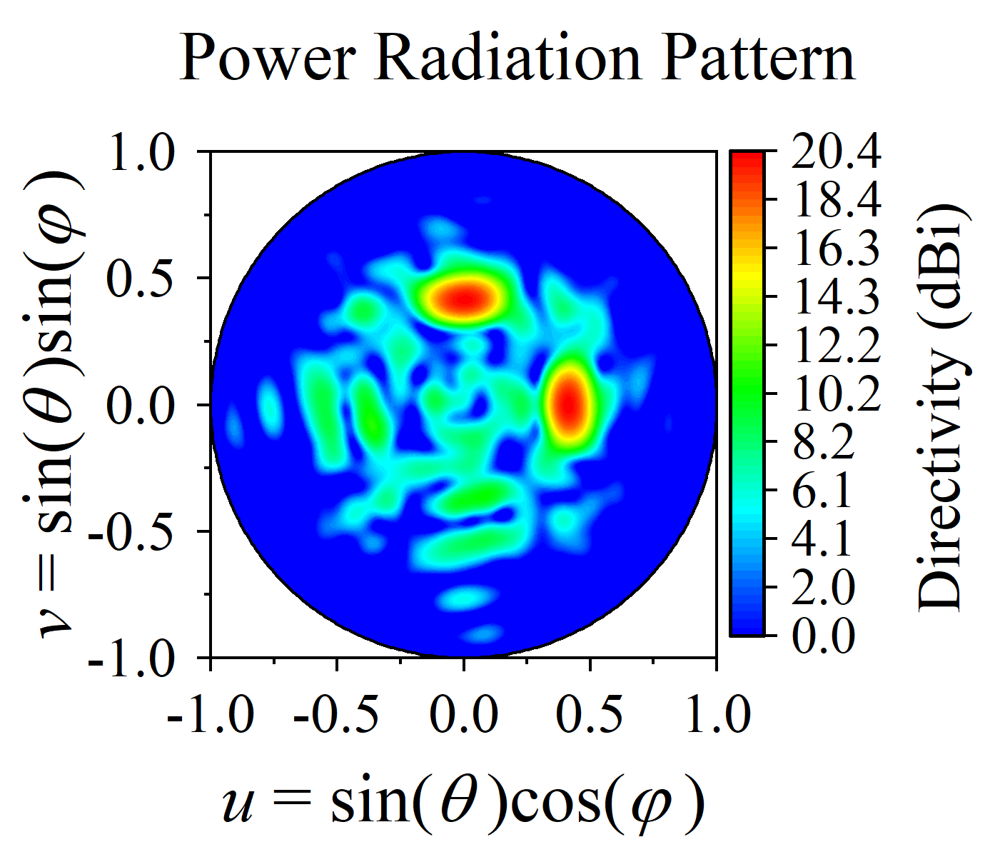
(c)

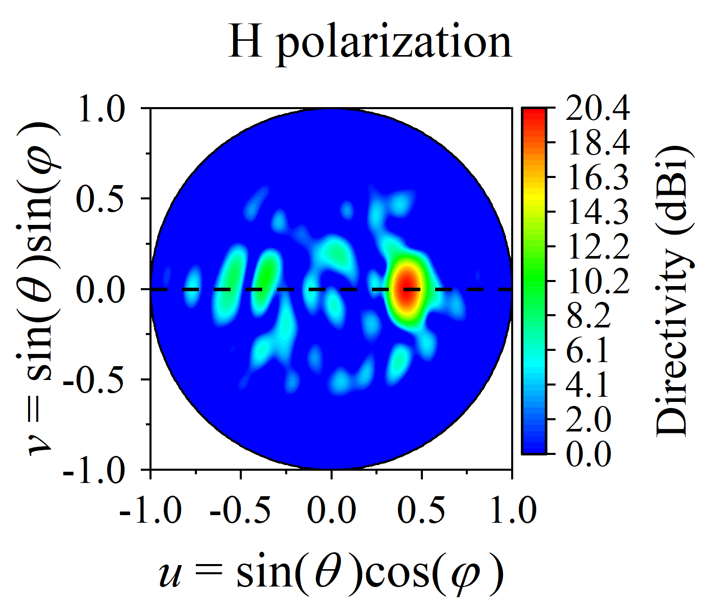
(d)

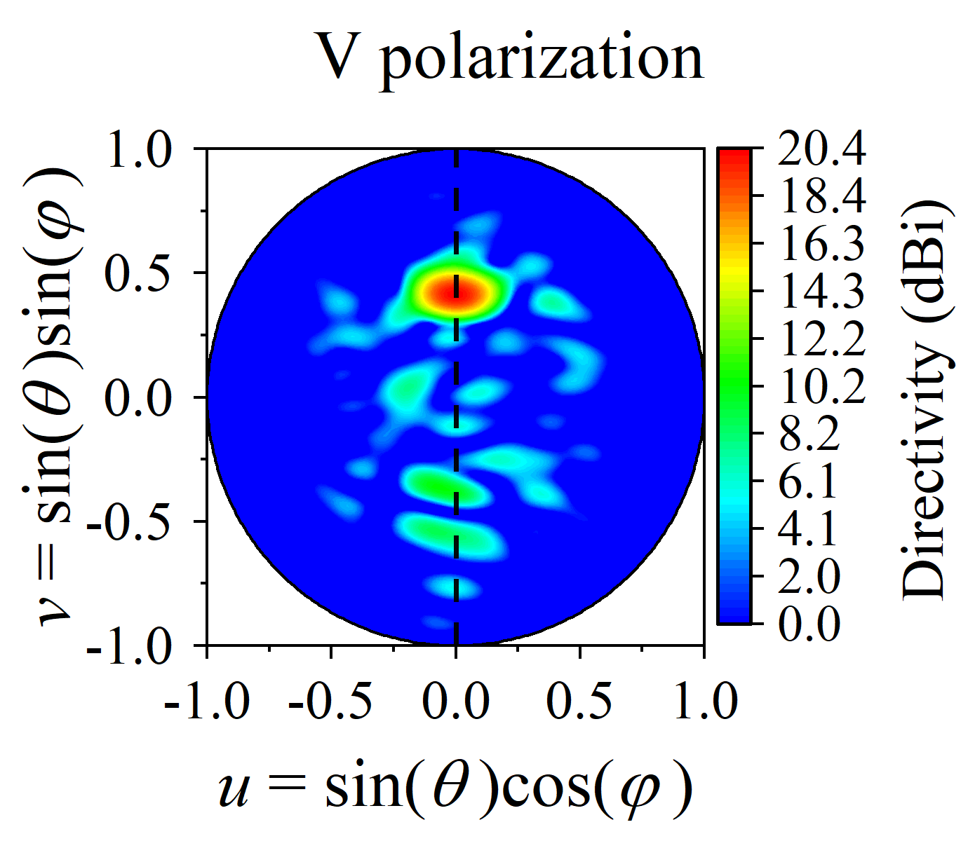
(e)

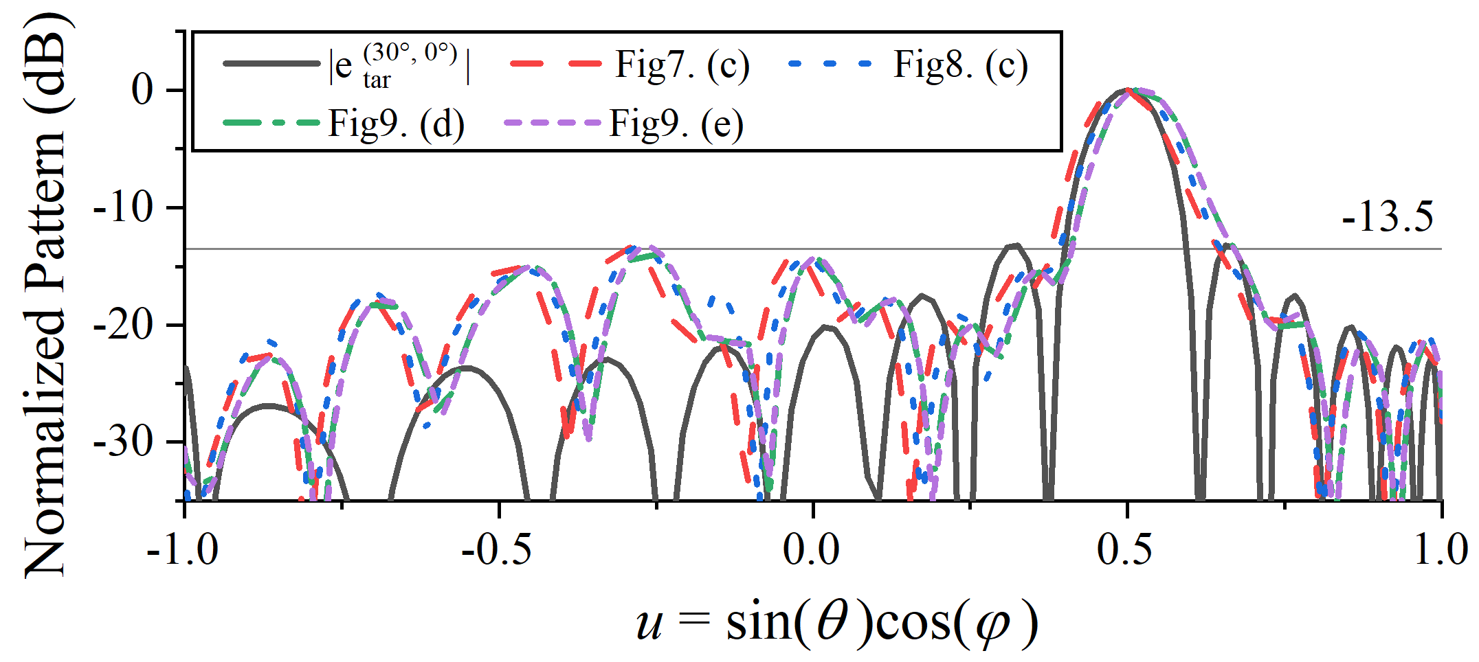
(f)

Figure 9: (a) Illustration and S-parameters of the array element (b) Schematic diagram of the dual-polarized sparse array; (c) Power radiation pattern; (d) Radiation pattern (H polarization); (e) Radiation pattern (V polarization); (f) 2D cut-plane at $v=0$: target vs. achieved.

V-D Other Potential Applications

V-D1 Flat Topped Beam

The IDMBSA is also suitable for designing special patterns, and it only requires modifying the target pattern. Here, we demonstrate a case using the flat topped beam (FTB) pattern as shown in Fig.10(a) as the target. The polarization constraint remains (13). The aperture field obtained using IDMBSA is denoted as $E_{\mathrm{ape},y}^{\mathrm{FTB}}$ as shown in Fig. 10(b, c). Its radiation pattern is shown in Fig. 10(d).

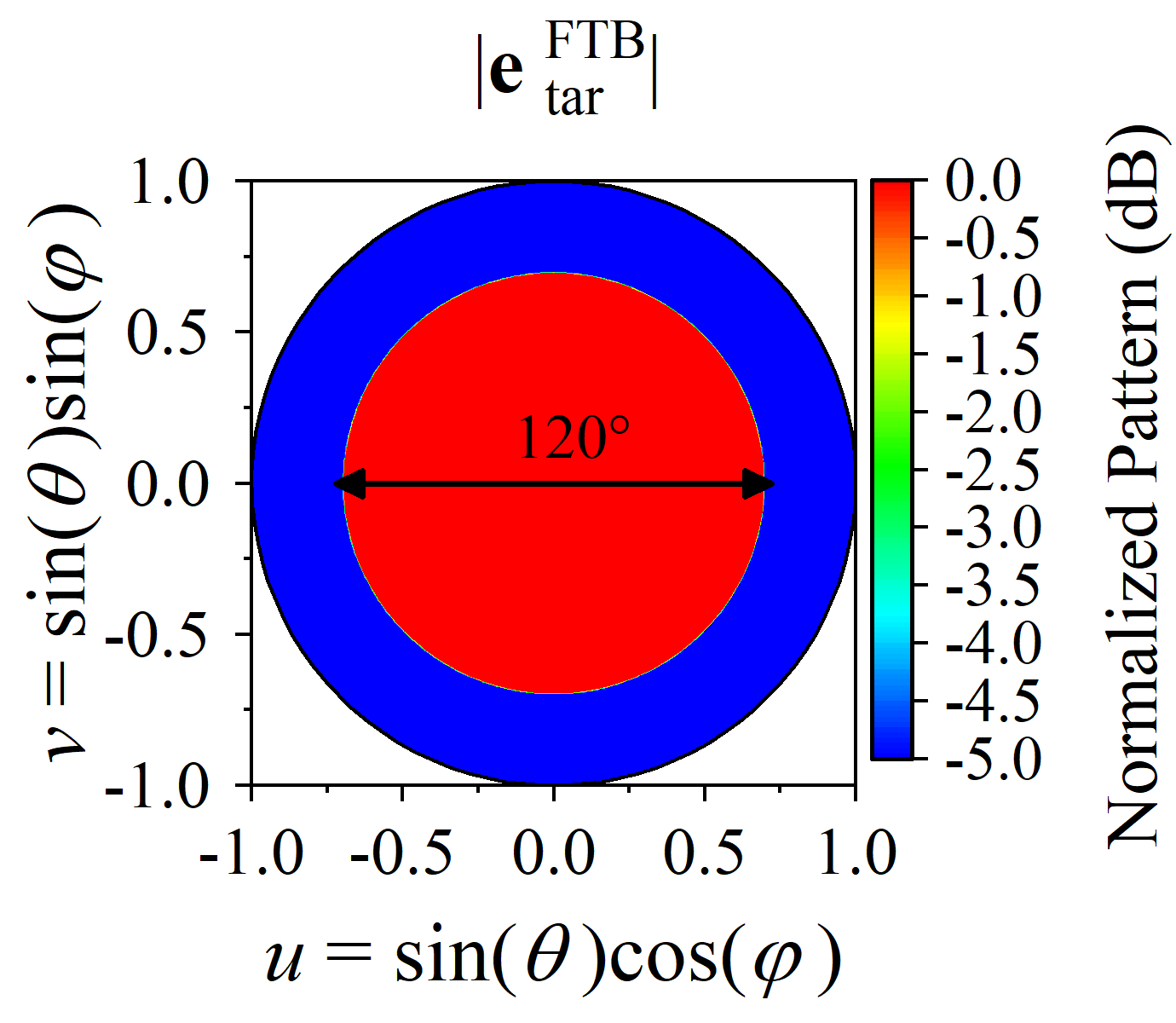
(a)

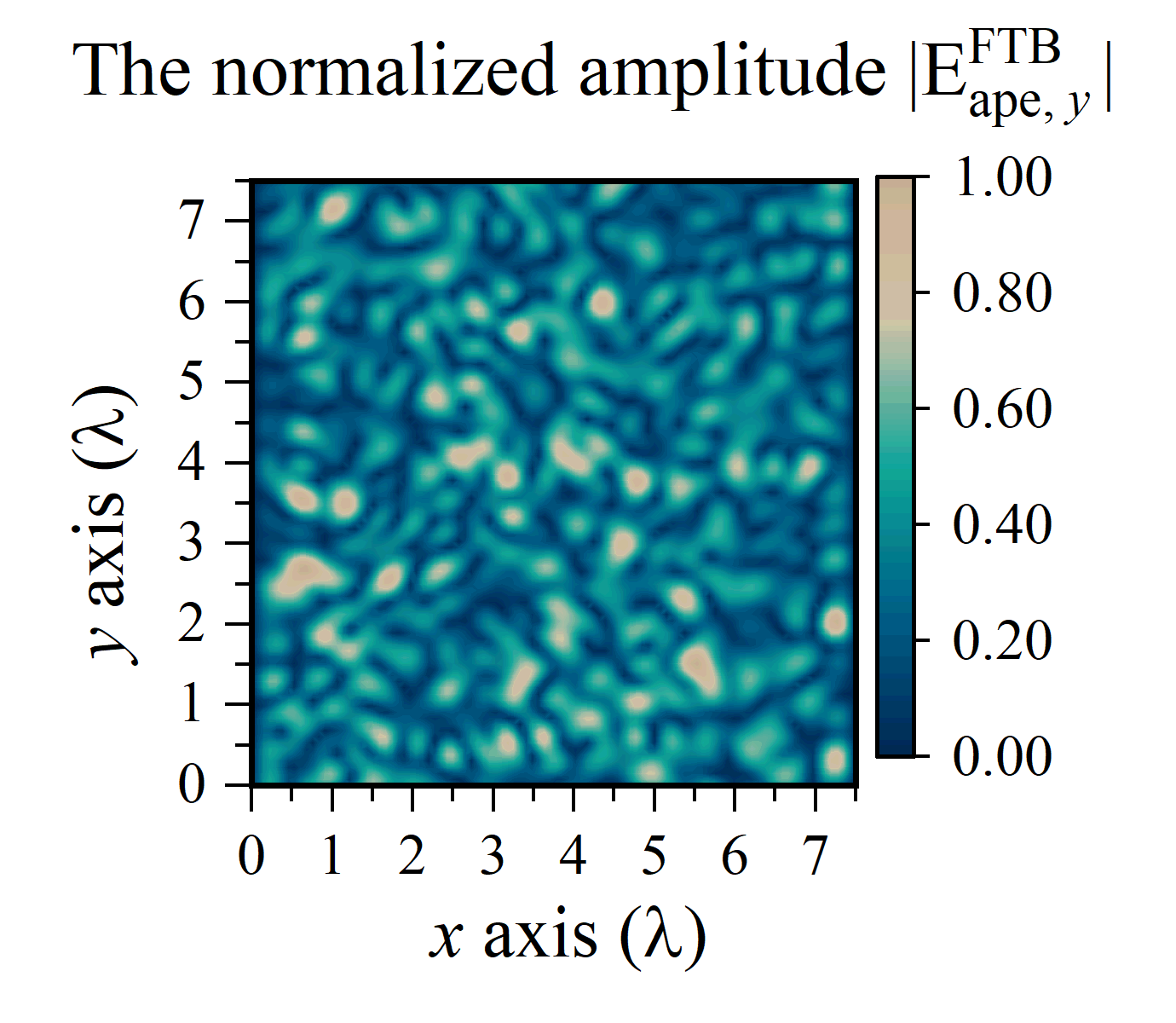
(b)

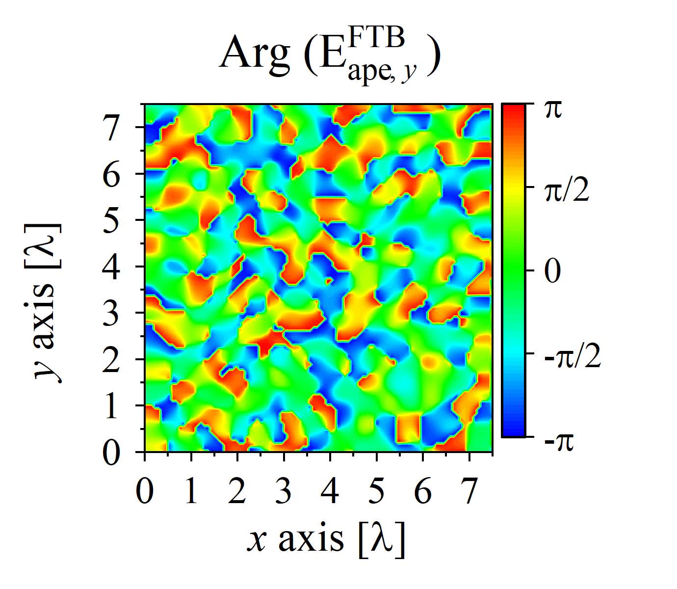
(c)

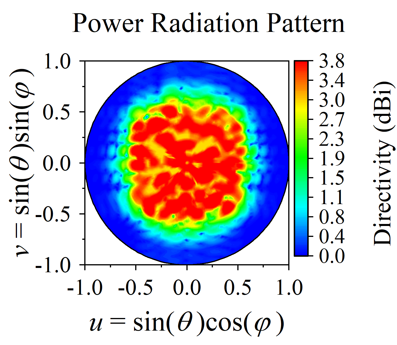
(d)

Figure 10: (a) Target FTB pattern; (b) $\left|E_{\mathrm{ape},y}^{\mathrm{FTB}}\right|$; (c) Arg $\left(E_{\mathrm{ape},y}^{\mathrm{FTB}}\right)$; (d) Power radiation pattern of $E_{\mathrm{ape},y}^{\mathrm{FTB}}$.

V-D2 Low Side Lobe Level

The side lobe level(SLL) in Fig. 5(d) and in Fig. 9 are not good. This is caused by using Fig. 3 as the target, rather than what IDMBSA brings. To handle this situation, simply use the ideal pattern like Fig. 11(a) as the target. The polarization constraint remains (13). The aperture field obtained by IDMBSA is denoted as $E_{\mathrm{SLL,ape},y}^{(60^{\circ},0^{\circ})}$ and shown in Fig. 11(b, c).

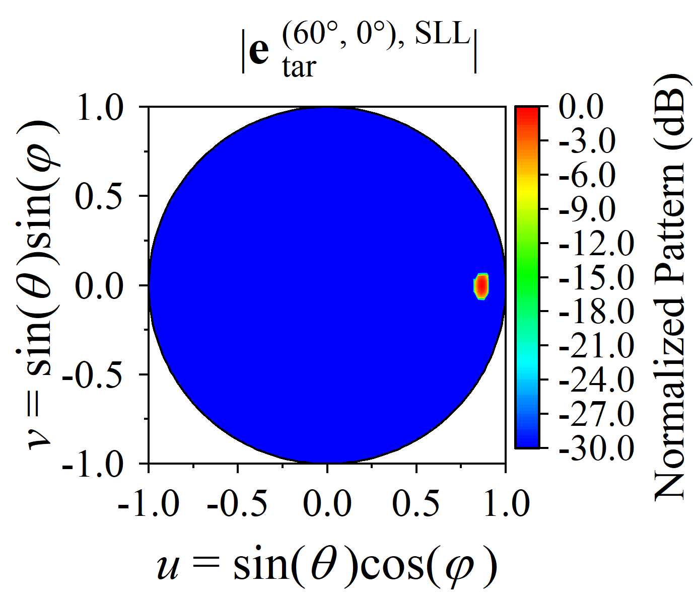
(a)

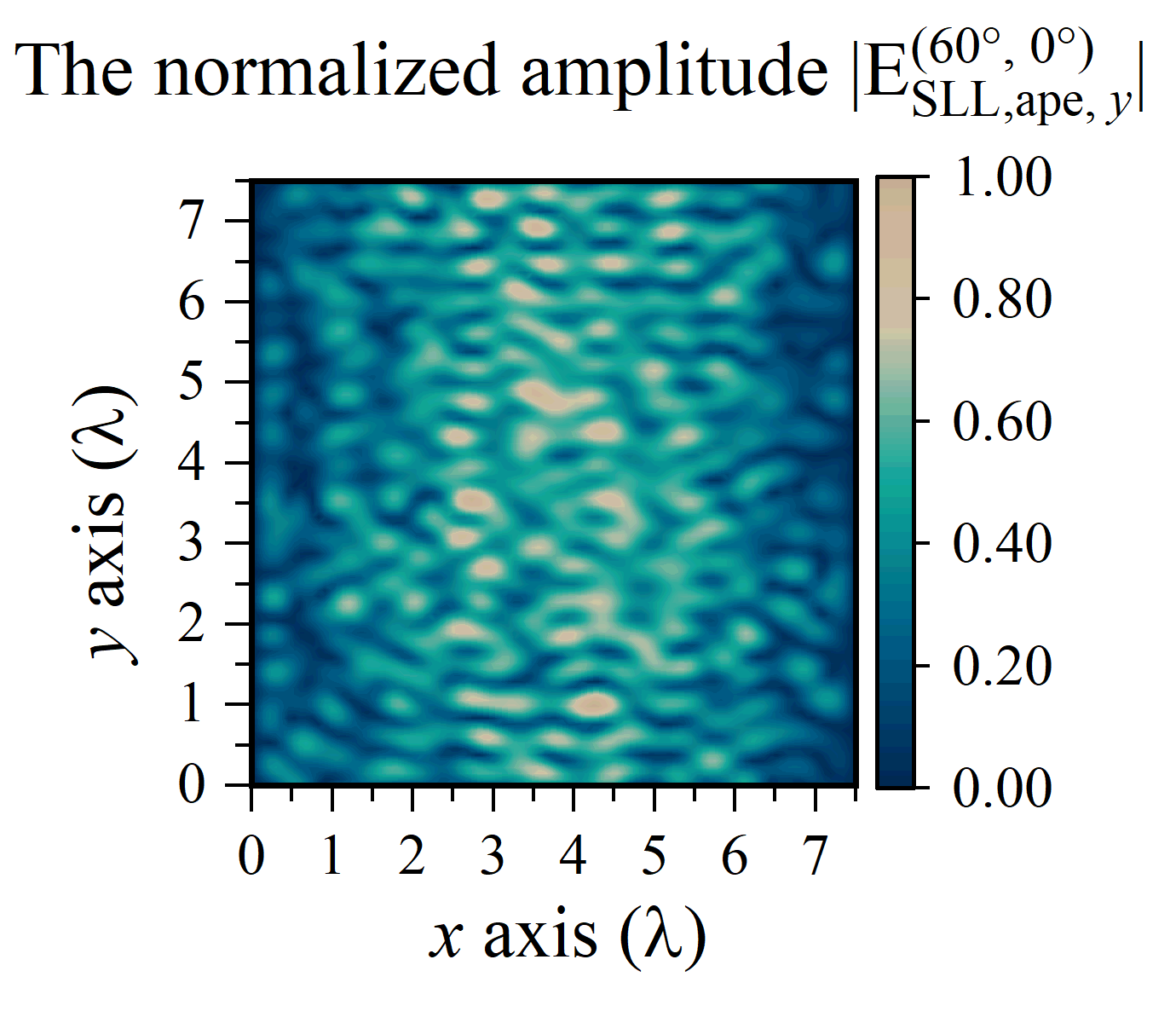
(b)

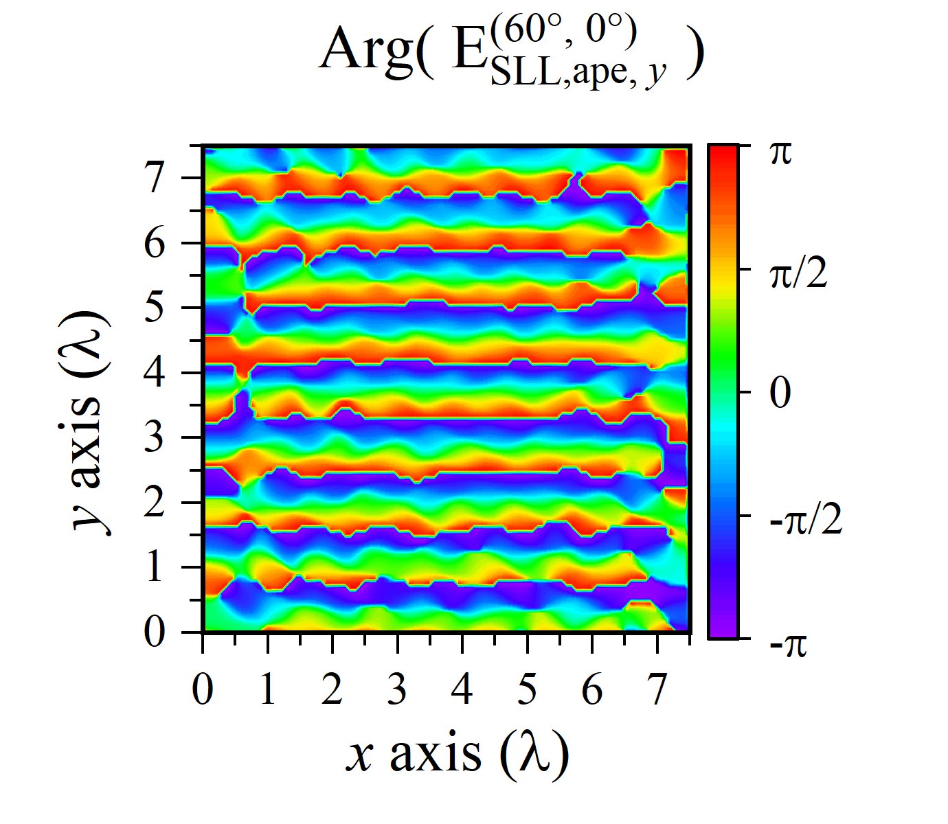
(c)

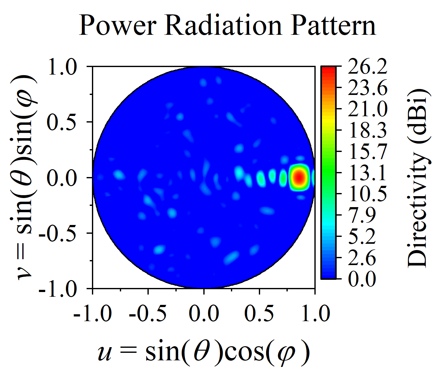
(d)

Figure 11: (a) Target pattern with low SLL; (b) $\left|E_{\mathrm{SLL,ape},y}^{(60^{\circ},0^{\circ})}\right|$; (c) Arg $\left(E_{\mathrm{SLL,ape},y}^{(60^{\circ},0^{\circ})}\right)$; (d) Power radiation pattern of $E_{\mathrm{SLL,ape},y}^{(60^{\circ},0^{\circ})}$.

V-D3 Large Aperture

Furthermore, IDMBSA remains applicable for large apertures. We once attempted to design a pencil beam pointing at 60 degrees on a super-sized aperture of 50 $\lambda$ and achieved excellent results. During this design process, we observed that a lower number of modes $M$ and $N$ made it difficult for the cost function to converge. However, once the number of modes exceeds a certain critical value (roughly 40), the cost function suddenly converges. This is an interesting phenomenon, and we believe it may hold significant implications for researching in performance limits.

V-D4 Transmitarray Antenna

IDMBSA can also be applied to the design of transmitting arrays. In such cases, it is necessary to consider the relative phase between the feeding antenna and the array elements and make appropriate adjustments. Detailed discussions and experimental validations can be found in the work of the authors [31], and we do not delve into further details here.

In addition, as mentioned in the Introduction, the aperture field distribution obtained by IDMBSA can also be used as a design objective for existing aperture field implementation methods [13] and [14]. By combining aperture field implementation methods and IDMBSA, it is possible to achieve the design of radiating devices with arbitrary far-field radiation pattern.

VI Conclusion

In this communication, we propose a method called IDMBSA for designing aperture field from arbitrary phaseless radiation pattern. The resulting aperture field obtained through IDMBSA, after discretization, can be used for traditional array synthesis. By applying suitable thresholding, it can be applied to sparse array design. Compared to traditional array synthesis methods and sparse array design methods, IDMBSA significantly reduces the dimensionality of the solution space. Furthermore, the utilization of analytical solutions further reduces the computational burden. Moreover, IDMBSA enables the independent design of dual-polarization radiation patterns. We have validated these through numerical and full-wave simulations, which show excellent agreement with the expected outcomes. Additionally, the smoothness of the aperture field obtained by IDMBSA makes it suitable as a design objective for existing aperture field implementation methods such as [13] and [14]. By combining these methods, it is possible to achieve the direct design of radiating devices from arbitrary phaseless far-field radiation pattern. However, there is still much follow-up work to be done, such as determining the limits of achievable radiation pattern complexity with finite apertures. These research will contribute to further advancing the application of IDMBSA in electromagnetic device design.

Appendix A Analytical expression of Equation (11)

Equation (15) is the analytic expression of (11).

$$|f_{x}(\theta,\phi)|=|\sum_{n=1}^{N} \left(\sum_{m=1}^{M}\alpha_{mn}^{x}\prod_{i=1}^{3}{g_{1,i}}\left(m,n,\theta,\phi\right)\right.$$ (15a)

$$\left.+\sum_{m=0}^{M}\beta_{mn}^{x}\prod_{i=1}^{3}{g_{2,i}}\left(m,n,\theta,\phi\right)\right)|$$

$$|f_{y}(\theta,\phi)|=|\sum_{m=1}^{M} \left(\sum_{n=1}^{N}\alpha_{mn}^{y}\prod_{i=1}^{3}{g_{1,i}}\left(m,n,\theta,\phi\right)\right.$$ (15b)

$$\left.+\sum_{n=0}^{N}\beta_{mn}^{y}\prod_{i=1}^{3}{g_{3,i}}\left(m,n,\theta,\phi\right)\right)|$$

where $g_{j,i}$ are defined in (16).

$$\chi_{1}=\sin\theta\sin\phi$$ (16a)

$$\chi_{2}=\sin\theta\cos\phi$$ (16b)

$$\begin{split}&g_{1,1}=\left(4abe^{-\frac{1}{2}jk\cos\phi\left(b\cos\theta+a\sin\theta\right)}\right)\\ &\quad\times\Big{[}\left(4n^{2}\pi^{2}+b^{2}k^{2}\left(\cos\left(2\phi\right)+2\cos\left(2\theta\right)\sin^{2}\left(\phi\right)-1\right)\right)\Big{.}\\ &\quad\Big{.}\times\left(a^{2}k^{2}\chi_{2}^{2}-m^{2}\pi^{2}\right)\Big{]}^{-1}\end{split}$$ (16c)

$$g_{1,2}=\left(-m\pi+e^{jka\chi_{2}}\left(m\pi\cos\left(m\pi\right)-jak\sin\left(m\pi\right)\chi_{2}\right)\right)$$ (16d)

$$\begin{split}&g_{1,3}=\left(e^{\frac{1}{2}jkb\cos\left(\phi+\theta\right)}n\pi\right.\\ &\qquad\quad\left.+e^{\frac{1}{2}jkb\cos\left(\phi-\theta\right)}\left(-n\pi\cos\left(n\pi\right)+jbk\sin\left(n\pi\right)\chi_{1}\right)\right)\end{split}$$ (16e)

$$g_{3,1}=g_{2,1}=g_{1,1}$$ (16f)

$$g_{2,2}=\left(-ak\chi_{2}+e^{jka\chi_{2}}\left(-jm\pi\sin\left(m\pi\right)+ak\cos\left(m\pi\right)\chi_{2}\right)\right)$$ (16g)

$$g_{2,3}=-jg_{1,3}$$ (16h)

$$g_{3,2}=\left(-jm\pi+e^{jka\chi_{2}}\left(jm\pi\cos\left(m\pi\right)+ak\sin\left(m\pi\right)\chi_{2}\right)\right)$$ (16i)

$$\begin{split}&g_{3,3}=\left(-bk\chi_{1}e^{\frac{1}{2}jkb\cos\left(\phi+\theta\right)}\right.\\ &\qquad\quad\ \left.+e^{\frac{1}{2}jkb\cos\left(\phi-\theta\right)}\left(-jn\pi\sin\left(n\pi\right)+bk\cos\left(n\pi\right)\chi_{1}\right)\right)\end{split}$$ (16j)

References

- [1] O. M. Bucci, G. Franceschetti, G. Mazzarella, and G. Panariello, “Intersection approach to array pattern synthesis,” IEE Proceedings H (Microwaves, Antennas and Propagation), vol. 137, no. 6, pp. 349–357(8), Dec. 1990.
- [2] O. M. Bucci, G. D’Elia, G. Mazzarella, and G. Panariello, “Antenna pattern synthesis: a new general approach,” Proceedings of the IEEE, vol. 82, no. 3, pp. 358–371, Mar. 1994.
- [3] O. M. Bucci, G. D’Elia, and G. Mazzarella, “Power synthesis of conformal arrays by a generalised projection method,” IEE Proceedings - Microwaves, Antennas and Propagation, vol. 142, no. 6, pp. 467–471(4), Dec. 1995.
- [4] Y.-Y. Bai, S. Xiao, C. Liu, and B.-Z. Wang, “A hybrid IWO/PSO algorithm for pattern synthesis of conformal phased arrays,” IEEE Transactions on Antennas and Propagation, vol. 61, no. 4, pp. 2328–2332, Apr. 2013.
- [5] O. M. Bucci and D. Pinchera, “A generalized hybrid approach for the synthesis of uniform amplitude pencil beam ring-arrays,” IEEE Transactions on Antennas and Propagation, vol. 60, no. 1, pp. 174–183, Jan. 2012.
- [6] P. Nayeri, F. Yang, and A. Z. Elsherbeni, “Design of single-feed reflectarray antennas with asymmetric multiple beams using the particle swarm optimization method,” IEEE Transactions on Antennas and Propagation, vol. 61, no. 9, pp. 4598–4605, Sep. 2013.
- [7] M. Khalaj-Amirhosseini, “Phase-only power pattern synthesis of linear arrays using autocorrelation matching method,” IEEE Antennas and Wireless Propagation Letters, vol. 18, no. 7, pp. 1487–1491, Jul. 2019.
- [8] S. Prasad, M. Meenakshi, and P. Rao, “Shaped beam from multiple beams using planar phased arrays,” Journal of Electromagnetic Waves and Applications, vol. 37, no. 4, pp. 592–604, Mar. 2023.
- [9] F. Yang, Y. Ma, Y. Chen, S. Qu, and S. Yang, “A novel method for maximum directivity synthesis of irregular phased arrays,” IEEE Transactions on Antennas and Propagation, vol. 70, no. 6, pp. 4426–4438, Jun. 2022.
- [10] S. L. Liu, X. Q. Lin, Y. H. Yan, and Y. L. Fan, “Generation of a high-gain bidirectional transmit–reflect-array antenna with asymmetric beams using sparse-array method,” IEEE Transactions on Antennas and Propagation, vol. 69, no. 9, pp. 6087–6092, Sep. 2021.
- [11] Z. N. Chen, “Metantennas: From patch antennas to metasurface mosaic antennas (invited paper),” in 2020 IEEE Asia-Pacific Microwave Conference (APMC), Dec. 2020, pp. 363–365.
- [12] J. W. Wu, Z. X. Wang, R. Y. Wu, H. Xu, Q. Cheng, and T. J. Cui, “Simple and comprehensive strategy to synthesize Huygens metasurface antenna and verification,” IEEE Transactions on Antennas and Propagation, vol. 71, no. 8, pp. 6652–6666, Aug. 2023.
- [13] M. Teniou, H. Roussel, N. Capet, G.-P. Piau, and M. Casaletti, “Implementation of radiating aperture field distribution using tensorial metasurfaces,” IEEE Transactions on Antennas and Propagation, vol. 65, no. 11, pp. 5895–5907, Nov. 2017.
- [14] A. Epstein and G. V. Eleftheriades, “Arbitrary antenna arrays without feed networks based on cavity-excited omega-bianisotropic metasurfaces,” IEEE Transactions on Antennas and Propagation, vol. 65, no. 4, pp. 1749–1756, Apr. 2017.
- [15] D. Wang, D. Tan, and L. Liu, “Particle swarm optimization algorithm: an overview,” Soft Computing, vol. 22, no. 2, pp. 387–408, Jan. 2018.
- [16] Y. Zhang, S. Wang, and G. Ji, “A comprehensive survey on particle swarm optimization algorithm and its applications,” Mathematical Problems in Engineering, vol. 2015, Oct. 2015, Art. no. 931256.
- [17] S. Katoch, S. S. Chauhan, and V. Kumar, “A review on genetic algorithm: past, present, and future,” Multimedia Tools and Applications, vol. 80, no. 5, pp. 8091–8126, Feb. 2021.
- [18] B. Fuchs, “Application of convex relaxation to array synthesis problems,” IEEE Transactions on Antennas and Propagation, vol. 62, no. 2, pp. 634–640, Feb. 2014.
- [19] S. Pearson and S. V. Hum, “Optimization of electromagnetic metasurface parameters satisfying far-field criteria,” IEEE Transactions on Antennas and Propagation, vol. 70, no. 5, pp. 3477–3488, May. 2022.
- [20] I. Iliopoulos, M. Teniou, M. Casaletti, P. Potier, P. Pouliguen, R. Sauleau, and M. Ettorre, “Near-field multibeam generation by tensorial metasurfaces,” IEEE Transactions on Antennas and Propagation, vol. 67, no. 9, pp. 6068–6075, Sep. 2019.
- [21] C.-S. Chen, B.-Z. Wang, and R. Wang, “Conversion method between port field and internal field of electromagnetic device based on time-reversal technique,” (in Chinese), ACTA PHYSICA SINICA, vol. 70, no. 7, pp. 070201–1, Apr. 2021, Art no. 20201682.
- [22] T. Brown, C. Narendra, Y. Vahabzadeh, C. Caloz, and P. Mojabi, “On the use of electromagnetic inversion for metasurface design,” IEEE Transactions on Antennas and Propagation, vol. 68, no. 3, pp. 1812-1824, Mar. 2020.
- [23] R. E. Collin, “Variational Methods for Waveguide Discontinuities, ”in Field theory of guided waves, 2nd ed. New York, NY, USA: Wiley, 1990, pp. 569–572.
- [24] J. Roy and L. Shafai, “Generalization of the Ludwig-3 definition for linear copolarization and cross polarization,” IEEE Transactions on Antennas and Propagation, vol. 49, no. 6, pp. 1006–1010, Jun. 2001.
- [25] M. Sørensen, H. Kajbaf, V. V. Khilkevich, L. Zhang, and D. Pommerenke, “Analysis of the effect on image quality of different scanning point selection methods in sparse ESM,” IEEE Transactions on Electromagnetic Compatibility, vol. 61, no. 6, pp. 1823–1831, Dec. 2019.
- [26] C. A. Balanis, “Appendix VIII: Method of Stationary Phase, ”in Antenna theory: analysis and design, 4th ed. Hoboken, NJ, USA: Wiley, 2016, pp. 1055–1059.
- [27] D. Yuan and X. Zhang, “An overview of numerical methods for the first kind Fredholm integral equation,” SN Applied Sciences, vol. 1, no. 10, p. 1178, Oct. 2019.
- [28] C.-S. Chen, R. Wang, J.-P. Liu, and B.-Z. Wang, Jun. 2023, “IDMBSA simulation data and part of the code,” IEEE Dataport, doi: https://dx.doi.org/10.21227/5sb9-4p13
- [29] Y.-F. Cheng, W. Shao, S.-J. Zhang, and Y.-P. Li, “An improved multi-objective genetic algorithm for large planar array thinning,” IEEE Transactions on Magnetics, vol. 52, no. 3, pp. 1–4, Mar. 2016.
- [30] B.-F. Sun, X. Ding, Y.-F. Cheng, and W. Shao, “Substrate integrated waveguide-slot wide-angle scanning aperiodic phased array with low side-lobe levels,” Microwave and Optical Technology Letters, vol. 62, no. 1, pp. 210–216, Jan. 2020.
- [31] C.-S. Chen, J.-P. Liu, R. Wang, and B.-Z. Wang, “The physical implementation of electromagnetic inverse design method based on metal-only transmitarray antenna,” in 2023 Int. Conf. Microwave and Millimeter Wave Technology (ICMMT 2023), QINGDAO, China, May. 2023, pp. 1–3, doi: 10.1109/ICMMT58241.2023.10277587.