Interference-Aware Constellation Design for Z-Interference Channels with Imperfect CSI

Abstract

A deep autoencoder (DAE)-based end-to-end communication over the two-user Z-interference channel (ZIC) with finite-alphabet inputs is designed in this paper. The design is for imperfect channel state information (CSI) where both estimation and quantization errors exist. The proposed structure jointly optimizes the encoders and decoders to generate interference-aware constellations that adapt their shape to the interference intensity in order to minimize the bit error rate. A normalization layer is designed to guarantee an average power constraint in the DAE while allowing the architecture to generate constellations with nonuniform shapes. This brings further shaping gain compared to standard uniform constellations such as quadrature amplitude modulation. The performance of the DAE-ZIC is compared with two conventional methods, i.e., standard and rotated constellations. The proposed structure significantly enhances the performance of the ZIC. Simulation results confirm bit error rate reduction in all interference regimes (weak, moderate, and strong). At a signal-to-noise ratio of $\rm 20dB$, the improvements reach about two orders of magnitude when only quantization error exists, indicating that the DAE-ZIC is highly robust to the interference compared to the conventional methods.

I Introduction

Interference is a central issue in today’s multi-cell networks. The information-theoretic model for a multi-cell network is the interference channel (IC). There have been many efforts to find the capacity of the IC either with the same generality and accuracy used by Shannon for point-to-point systems [1, 2] or by seeking approximate solutions with a guaranteed gap to optimality at any signal-to-noise ratio (SNR) [3]. However, the capacity region of the two-user IC is only known for strong interference where decoding and canceling the interference is optimal [1]. Also, at very weak interference, sum-capacity is achievable by treating interference as noise [4]. In general, Han-Kobayashi encoding is the best achievable scheme [2], which decodes part of the interference and treats the remaining as noise.

The aforementioned Shannon-theoretic works are based on Gaussian inputs. Despite being theoretically optimal, Gaussian alphabets are continuous and unbounded, and thus, are rarely applied in real-world communication. In practice, signals are generated using finite alphabet sets, such as phase-shift keying (PSK) and quadrature amplitude modulations (QAM). The performance gap between the finite alphabet input and the Gaussian input design is non-negligible [5]. However, conventional finite-alphabet approaches are based on predefined uniform constellations like QAM. These constellations are defined for point-to-point systems [6, 7, 8] and their constellation shaping is oblivious to interference. Such an inability to respond to interference is an obstacle to improving the bit-error rate and spectral efficiency of today’s interference-limited communication systems.

In this paper, we consider the two-user one-sided IC, also known as the Z-interference channel (ZIC) [9], with imperfect CSI. Previous works have examined the ZIC with finite alphabet inputs and uniform constellations in certain regimes. In [10], it is shown that rotating one input constellation (alphabet) can improve the sum-rate of the two-user IC in strong/very strong interference regimes. Later, an exhaustive search for finding the optimal rotation of the signal constellation was presented in [11]. The focus of the above papers is to maximize the achievable rates, and they do not study bit-error rate (BER) performance. BER is a critical metric, and interference can severely increase the BER by distorting the received constellation when uniform constellations like QAM are employed.

Deep autoencoder (DAE)-based end-to-end communication is an emerging approach to finite-alphabet communication in which BER is the main performance measure and constellation design is inherent to it. Various groups have proposed DAE-based communication both for single- and multi-user systems [12, 14, 13]. Particularly, [12, 15, 16] have studied communication over the IC. These works, however, are only for the symmetric interference case and compare their results with simple baselines (e.g., quadrature phase shift keying (QPSK)), but we know QPSK performs much poorer than a rotated QPSK [10, 11]. In addition, those structures assume perfect knowledge of channel state information (CSI), but the extension from perfect CSI to imperfect CSI is not straightforward and has not been explored.

This paper sheds light on DAE-based communication over asymmetric interference with both perfect and imperfect CSI. Specifically, we design and train novel DAE-based architectures for the ZIC with finite-alphabet inputs. In this architecture, we have two transmitter-receiver DAE pairs that work together to mitigate interference and adapt the constellation to the interference intensity, leading to improved BER. Key contributions of the paper are as follows:

• We design a DAE-based transmission structure for the ZIC which works both for imperfect and perfect CSI at different interference regimes, including weak, moderate, and strong interference. In the proposed architecture, we have designed an average power constraint normalization layer to allow generating nonuniform constellations to use the in-phase and quadrature-phase (I/Q) plane efficiently. The resulting constellations are adaptive to the interference intensity and morph in a way that the receivers see distinguishable symbols.

• This is the first study examining finite-alphabet ZIC under imperfect CSI. We consider both estimation and quantization errors. Particularly, the CSI estimation error confuses the DAE and brings difficulty in training and testing performance. The quantization error, coming from the limited feedback channel capacity, is an additional error that brings unwanted rotations to the constellations. To overcome these challenges, we first simplify the CSI parameters by designing an equivalent system model and then we build the DAE to reduce the BER.

For benchmarking, we use rotated uniform constellations which are more competitive than unrotated constellations. The proposed DAE-ZIC shows significantly better BER performance for all interference regimes (weak, moderate, and strong interference). The overall BER reduction is about 40%, and the gap between the DAE-ZIC and the best conventional method is even larger when quantization error exists.

We organize the remainder of this paper as follows. We first elaborate on the ZIC system model and its simplification in Section II. We next introduce the DAE design and the training approach in Section III. We present the simulation results and conclusions in Sections IV and V, respectively.

II System Model with Imperfect CSI

II-A Channel Model of the ZIC

The system model of two-user single-input single-output ZIC is shown in Fig. 1. The two transmitter-receiver pairs wish to reliably transmit their messages while the transmission of the first pair is interfered with by the second one. The four nodes are named Tx1, Tx2, Rx1, and Rx2. The received signals at Rx1, and Rx2 can be written as

$$y_{1}=h_{11}x_{1}+h_{21}x_{2}+n_{1},$$ (1a)

$$y_{2}=h_{22}x_{2}+n_{2},$$ (1b)

in which $x_{i}$ and $y_{i}$, $i\in\{1,2\}$, denote the transmitted and received symbols, $n_{i}$ is white Gaussian noise with mean zero and variance $\sigma_{i}^{2}$, and actual channel coefficients are given by

$$h_{ij}\sim\mathcal{CN}(\mu_{H},\sigma_{H}^{2}),\;i,j\in\{1,2\},$$ (2)

where $\mu_{H}$ and $\sigma_{H}^{2}$ are the mean and variance of the channel. $h_{12}=0$ by the definition of the ZIC. The interference intensity is defined as

$$\alpha\triangleq\left|{h_{21}}{h_{11}^{-1}}\right|^{2}.$$ (3)

In practice, perfect channel gains are not available. ${h}_{11}$ and ${h}_{21}$ are estimated by Rx1 whereas ${h}_{22}$ is estimated by Rx2. The CSI imperfectness comes from two sources: 1) the error in the CSI estimation at the receivers’ side and 2) the quantization error when feeding CSI back to the transmitters. We give the details of two types of errors as follows.

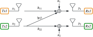
Figure 1: Original system model of the ZIC where $h_{ij}=r_{ij}e^{j\theta_{ij}}$.

II-A1 Estimation Errors

The estimated channel coefficients are determined by the actual channel and estimation error, which is modeled as [17]

$$\hat{h}_{ij}=\hat{r}_{ij}e^{j\hat{\theta}_{ij}}\triangleq{h}_{ij}-\varepsilon_{ij},\;i,j\in\{1,2\},$$ (4)

where $\hat{r}_{ij}$ and $\hat{\theta}_{ij}$ are amplitude and phase of $\hat{h}_{ij}$, $h_{ij}$ is the actual channel, and

$$\varepsilon_{ij}\sim\mathcal{CN}(0,\sigma_{E}^{2})$$ (5)

is the estimation error with the variance $\sigma_{E}^{2}$. Hence, we have $\hat{h}_{ij}\sim\mathcal{CN}(\mu_{H},\sigma_{H}^{2}+\sigma_{E}^{2})$. The imperfectness of $h_{ij}$ affects the decoding process.

II-A2 Quantization Errors

The transmitters require the knowledge of CSI in closed-loop systems. However, due to the limited feedback resources, the feedback information is quantized with reduced accuracy. Thus, quantization brings in another imperfectness. For example, Rx1 estimates ${h}_{11}$ and ${h}_{21}$ and gets the estimated interference intensity, $\hat{\alpha}=|\hat{h}_{21}\hat{h}_{11}^{-1}|^{2}$. To let all four nodes access $\hat{\alpha}$, a quantized value of that

$$\alpha_{q}=Q(\hat{\alpha}),$$ (6)

is fed back to Tx1, Tx2, and Rx2, where $Q(\cdot)$ is a quantizer of its input variable. $Q(\cdot)$ uniformly divides the considered range of $\hat{\alpha}$, which is $[0,3]$, into $2^{N_{q}}$ segments. The middle value of the segment is the quantization result.

II-B Simplified Model of the ZIC

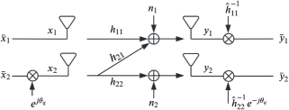
Figure 2: Pre- and post-processed model of the ZIC to simplify it (see Remark 1) for a DAE-based implementation.

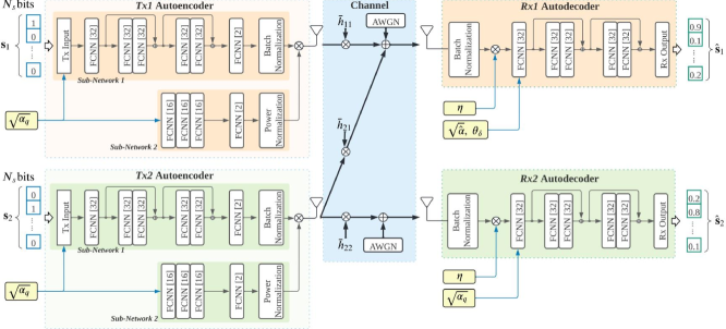
Figure 3: The architecture of the two-user DAE-ZIC implemented by two pairs of deep autoencoders. Each transmitter of the ZIC contains two sub-networks. Sub-network 1 mainly generates the constellation and sub-network 2 is used to implement the average power constraint. The receivers decode their bits from the received signal. $\eta$ is a power control parameter in (15).

In this subsection, we simplify the above model for DAE. Such a model shown in Fig. 2 is achieved by pre- and post-processing in Tx2, Rx1, and Rx2. Specifically, Tx2 applies pre-processing by multiplying $e^{j\theta_{q}}$ to the source signal defined as $\bar{x}_{2}$, i.e., $x_{2}=\bar{x}_{2}e^{j\theta_{q}}$. $\theta_{q}$ is estimated by Rx1 and fed back to other nodes designed as

$$\theta_{q}\triangleq Q(\hat{\theta}_{11}-\hat{\theta}_{21})=(\hat{\theta}_{11}-\hat{\theta}_{21})+\theta_{\delta},$$ (7)

where $\hat{\theta}_{11}$ and $\hat{\theta}_{21}$ are defined in (4), and $\theta_{\delta}$ is the quantization error. Correspondingly, ${x}_{1}=\bar{x}_{1}$ since $h_{12}=0$. The received signals after post-processing are

$$\bar{y}_{1}=\bar{h}_{11}\bar{x}_{1}+\bar{h}_{21}\bar{x}_{2}+\bar{n}_{1},$$ (8a)

$$\bar{y}_{2}=\bar{h}_{22}\bar{x}_{2}+\bar{n}_{2},$$ (8b)

where the equivalent channels are given by

$$\bar{h}_{ii}\triangleq{h}_{ii}\hat{h}_{ii}^{-1}=1+\varepsilon_{ii}\hat{h}_{ii}^{-1},\;$$ (9a)

$$\bar{h}_{21}\triangleq{h}_{21}\hat{h}_{11}^{-1}e^{j\theta_{q}}=\sqrt{\hat{\alpha}}e^{j\theta_{\delta}}+\varepsilon_{21}\hat{h}_{11}^{-1}e^{j\theta_{q}},$$ (9b)

and $\bar{n}_{i}$ is the equivalent noise which is given by

$$\bar{n}_{i}\triangleq n_{i}\hat{h}_{ii}^{-1}\sim\mathcal{CN}(0,\sigma_{N}^{2}\hat{r}_{ii}^{-2}).$$ (10)

Remark 1

If the estimation error and the quantization error are absent, i.e., $\varepsilon_{ij}=0$ and $\theta_{\delta}=0$, the system in (8a)-(8b) reduces to the one with perfect CSI case [9, 18, 19], in which the channel gains of the direct and interference links become $\bar{h}_{ii}=1$ and $\bar{h}_{21}=\sqrt{\alpha}$. These are all real-valued.

III Deep Autoencoder for ZIC for Imperfect CSI

Existing studies [10, 11] use standard QAM constellations for interference channels. Such constellations have fixed symbols and are not adjustable according to the interference intensity. To improve the transmission performance, we propose a DAE-based transmission for the two-user ZIC, named DAE-ZIC. We show the architecture in Fig. 3.

III-A The Architecture of DAE-ZIC

III-A1 Network Input

Each transmitter sends $N_{s}$ bits to the corresponding receiver. The feedback of the interference intensity $\sqrt{\alpha_{q}}$ is appended to the input bit vector. The two transmitters are expected to jointly design their constellations and the receivers will decode correspondingly.

III-A2 Transmitter DAE

As shown in Fig. 3, the DAE in each transmitter contains two sub-networks. Sub-network 1 converts the input bit-vector to symbols that take the value of $h_{21}$ into consideration. Sub-network 2 performs power allocation, which controls the power of the I/Q components.

The main components of sub-network 1 are are fully connected neural networks (FCNN), residual connections, and the output batch normalization (BN) layer. The activation function of the FCNN layers is tanh except for the last layer, which has two hidden nodes and no activation function. Assume the batch size is $N_{B}$, and the output of the last FCNN is $\mathbf{X}_{\textmd{fcnn}}\triangleq[\mathbf{x}_{\textmd{fcnn}}^{\textmd{I}},\;\mathbf{x}_{\textmd{fcnn}}^{\textmd{Q}}]$, where $\mathbf{x}_{\textmd{fcnn}}^{\textmd{I}}$ and $\mathbf{x}_{\textmd{fcnn}}^{\textmd{Q}}\in\mathbb{R}^{N_{B}\times 1}$ are the outputs of the two hidden nodes and represent I/Q of the complex-valued signal.

Since the FCNN has unbounded outputs, it cannot guarantee a power constraint at the transmitter. We propose a transmitter architecture as shown in Fig. 3 to achieve an average power constraint at each antenna. First, we use BN in sub-network 1 to unify the average power of I/Q independently. The BN layer linearly normalizes ${\mathbf{x}}_{\textmd{fcnn}}^{\textmd{I}}$ and ${\mathbf{x}}_{\textmd{fcnn}}^{\textmd{Q}}$, in which the normalized vectors $\mathbf{x}_{B}^{\textmd{I}}$ and $\mathbf{x}_{B}^{\textmd{Q}}$ are

$$\mathbf{x}_{B}^{\textmd{I}}\triangleq\beta^{\textmd{I}}{\mathbf{x}}_{\textmd{fcnn}}^{\textmd{I}},\;\text{and}\quad\mathbf{x}_{B}^{\textmd{Q}}\triangleq\beta^{\textmd{Q}}{\mathbf{x}}_{\textmd{fcnn}}^{\textmd{Q}},$$ (11)

where $\bm{\beta}\triangleq[\beta^{\textmd{I}},\;\beta^{\textmd{Q}}]^{T}$ contains two factors for normalization. Then, the powers of $\mathbf{x}_{B}^{\textmd{I}}$ and $\mathbf{x}_{B}^{\textmd{Q}}$ are modified by sub-network 2. Sub-network 2 has two output values: $\gamma^{\textmd{I}}$ and $\gamma^{\textmd{Q}}$. The FCNN layers in sub-network 2 determine the power allocated to the I/Q components based on the input value $\sqrt{\alpha}$. The power normalization (PN) block in sub-network 2 limits the total power to $P_{t}$. Defining ${\bm{\gamma}}\triangleq[\gamma^{\textmd{I}},\;\gamma^{\textmd{Q}}]^{T}\in\mathbb{R}^{2\times 1}$, we should have ${\bm{\gamma}}^{T}{\bm{\gamma}}=P_{t}$. Finally, the outputs of the BN and PN are multiplied together, i.e.,

$$\mathbf{x}_{\textmd{out}}^{\textmd{I}}\triangleq\gamma^{\textmd{I}}\mathbf{x}_{B}^{\textmd{I}},\;\text{and}\quad\mathbf{x}_{\textmd{out}}^{\textmd{Q}}\triangleq\gamma^{\textmd{Q}}\mathbf{x}_{B}^{\textmd{Q}}.$$ (12)

The powers of $\mathbf{x}_{\textmd{out}}^{\textmd{I}}$ and $\mathbf{x}_{\textmd{out}}^{\textmd{Q}}$ are $\gamma^{\textmd{I}}$ and $\gamma^{\textmd{Q}}$, respectively. To summarize, BN is applied to the I/Q components along the time, while PN normalizes the I/Q components at each time. Hence, the two normalization operations are implemented in different dimensions. In this way, the average power constraint is reached.

III-A3 Channel Implementation

The channels are implemented by FCNN layers independently. The weight, $\bar{\mathbf{H}}_{ij}$, is the real form of the channel $\bar{h}_{ij}=\bar{h}_{ij}^{\textmd{I}}+j\bar{h}_{ij}^{\textmd{Q}}$ in (9a)-(9b),

$$\bar{\mathbf{H}}_{ij}=\left[\begin{matrix}\bar{h}_{ij}^{\textmd{I}}&-\bar{h}_{ij}^{\textmd{Q}}\\ \bar{h}_{ij}^{\textmd{Q}}&\quad\bar{h}_{ij}^{\textmd{I}}\end{matrix}\right].$$ (13)

These channel layers have zero-bias, no activation function, and are non-trainable.

III-A4 Receiver DAE

The received signals are $\bar{y}_{1}$ and $\bar{y}_{2}$. To ensure the receiver networks have a finite input range, we use BN layers to unify the power of the received signals, i.e.,

$${y}_{\textmd{B},i}=\xi\bar{y}_{i},\;\;\mathbb{E}\{|{y}_{\textmd{B},i}|^{2}\}=1,\;\;\forall i\in\{1,2\},$$ (14)

where $\xi$ is a coefficient to reach the unit power. The process details and settings are the same as the ones in the transmitter.

We further define the desired signal for Rx1 as $x_{\textmd{D},1}\triangleq\bar{x}_{1}+\sqrt{\alpha}\bar{x}_{2}$ which contains the true desired signal $\bar{x}_{1}$ and the interference $\sqrt{\alpha}\bar{x}_{2}$. The goal of the receiver is to decode $x_{1}$ for an arbitrary $\bar{x}_{2}$ in its constellation. The desired signal of Rx2 is $x_{\textmd{D},2}\triangleq\bar{x}_{2}$. However, the normalization of the received signal (14) makes the power of the desired signal vary with the SNR. Hence, the autoencoder should adjust the decoding boundary according to the SNR, which is an extra burden. So, we turn to normalize the desired signal using a linear factor, $\eta$, multiplied by the batch normalization output, i.e.,

$$y_{\textmd{D},i}=\eta\cdot{y}_{\textmd{B},i},\;\eta\triangleq\sqrt{1+{P_{\textmd{D,i}}}{\sigma_{N}^{-2}}},\quad\forall i\in\{1,2\},$$ (15)

where $P_{\textmd{D},i}$ is the power of the desired signal $x_{\textmd{D},i}$ and $\sigma_{N}^{2}$ is the noise power. In short, the BN normalizes the desired signals using pre-processing $\eta$.

Besides, the receivers append the available parameters as additional input to the FCNN layer. Since the estimated interference intensity $\sqrt{\hat{\alpha}}$ and the quantization error of feedback angle $\theta_{\delta}$ are known at Rx1, we input these parameters to the autoencoder of Rx1. For Rx2, the feedback of the interference intensity $\sqrt{\alpha_{q}}$ is the additional input. The final output of the DAE is an estimation of the transmitted bit-vectors, $\hat{\mathbf{s}}_{1}$ and $\hat{\mathbf{s}}_{2}$, as shown in Fig. 3. The output layer uses soft-max. More specifically, the activation function is sigmoid.

Algorithm 1 Training Procedure for the DAE-ZIC

1:Inputs: $N_{s}$, $\alpha_{\min}$, $\alpha_{\max}$, $\mu_{H}$, $\sigma_{H}^{2}$, $\sigma_{E}^{2}$, $T$, and $N_{q}$.

2:Set $P_{t}=1$W, SNR$=10$dB, $N_{\alpha}=30,000$, $E_{p}=10$, $N_{B}=10^{4}$, and $l_{r}=10^{-2}$ which will drop to $d_{r}l_{r}=0.95l_{r}$ after every $N_{d}=200$ trained channels.

3:Initialize the DAE-ZIC network.

4:for index $i_{\alpha}$ from $1$ to $N_{\alpha}$ do

5:     Uniformly and randomly select one $\alpha\in[\alpha_{\min},\alpha_{\max}]$.

6:     while 1 do

7:         Randomly generate $h_{11}$ and $h_{22}$ using (2).

8:         Randomly generate $\varepsilon_{11}$, $\varepsilon_{22}$, and $\varepsilon_{21}$ using (5).

9:         If (17) satisfied, then Break.

10:     end while

11:     Uniformly generate $\Delta\theta_{q}$ in $\frac{1}{2^{N_{q}}}[-\pi,\pi]$.

12:     Update $\alpha_{q}$, $\theta_{\delta}$, and $\theta_{q}$ using (6) and (7).

13:     Normalize the channels using (9a) and (9b).

14:     for index $i_{e}$ from $1$ to $E_{p}$ do

15:         Randomly generate $N_{B}$ bit vectors.

16:         Update the weights of the DAE-ZIC using Adam.

17:     end for

18:     Set learning rate $l_{r}=d_{r}l_{r}$ if $i_{\alpha}/N_{d}$ is an integer.

19:end for

III-A5 Loss Function

In our DAE-ZIC, each receiver has its own estimation of the transmitted bits. Then, the overall loss function of the DAE-ZIC is $\mathcal{L}=\mathcal{L}_{1}+\mathcal{L}_{2}$, where $\mathcal{L}_{1}$ and $\mathcal{L}_{2}$ are the losses at Rx1 and Rx2. In this paper, we use binary cross-entropy as the loss function, i.e.,

$$\mathcal{L}_{i}=\frac{1}{N_{B}}\sum_{n=1}^{N_{B}}\mathbf{s}_{i,n}^{T}\log\hat{\mathbf{s}}_{i,n}+(1-\mathbf{s}_{i,n})^{T}\log(1-\hat{\mathbf{s}}_{i,n}),$$ (16)

where $i\in\{1,2\}$ distinguishes the users, $N_{B}$ is the batch size, $\mathbf{s}_{i,n}$ is the $n$th input bit-vector in the batch, and $\hat{\mathbf{s}}_{i,n}$ is corresponding the output. The loss function treats each element of the DAE output as a zero/one classification task. Cross-entropy is used to evaluate each classification task. Finally, the loss is the summation of the loss of $N_{s}$ tasks, where $N_{s}$ is the number of bits in the transmission. In the training process, the back propagation algorithm passes $\mathcal{L}_{1}$ to Rx1 and this will further go to Tx1 and Tx2. The $\mathcal{L}_{2}$ affects the Rx2 and Tx2.

III-B Training Procedure of the DAE-ZIC

We use separate instances of DAEs for different ranges of the interference gain $\alpha$. This is because training one network over all values of $\alpha$ is not easy. In each training, we select the $N_{s}$ and the desired range for $\alpha\in[\alpha_{\min},\alpha_{\max}]$. We train the DAE repeatedly using random values of $\alpha$ in this interval. For each $\alpha$, the DAE is trained through epochs $E_{p}$, mini-batch size $N_{B}$, and a constant learning rate $l_{r}$. After training the DAE for $N_{d}$ different values of $\alpha$, the learning rate is reduced to $d_{r}l_{r}$. The detailed training procedure is summarized in Algorithm 1. Also, we choose the best DAEs out of five individually trained networks with the same hyper parameters. The best is defined by the average loss on ten randomly generated values of $\alpha$ in $[\alpha_{\min},\alpha_{\max}]$. To avoid the numerical problem, in both training and testing, we only use channels satisfying

$$\max(\left|{\varepsilon_{11}}{\hat{h}_{11}^{-1}}\right|,\left|{\varepsilon_{22}}{\hat{h}_{22}^{-1}}\right|,\left|{\varepsilon_{21}}{\hat{h}_{11}^{-1}}\right|)<T,$$ (17)

where $T$ is a threshold. $T$ is set as one in this paper so that the estimation errors are not dominant in $\bar{h}_{ii}$ in (9a).

IV Performance Analysis

The performance is evaluated and compared for the three methods listed below. To be fair to the users, we the use maximum (worst) BER of the two as the measurement.

• DAE-ZIC: The proposed method which designs nonuniform constellations based on the interference intensity.

• Baseline-1: The transmitters directly use standard QAM.

• Baseline-2: Tx1 uses standard QAM, while Tx2 rotates the standard QAM symbols based on the interference intensity [11].

The implementation of DAEs are performed in TensorFlow and the baselines are performed in MATLAB.

IV-A CSI with Estimation Error

The received constellations at Rx1 generated by the baselines and the proposed DAE-ZIC are shown in Fig. 4. In this simulation, we set $N_{s}=2$, i.e., each user has $2^{N_{s}}=4$ information symbols. The estimated ${\hat{\alpha}}$ and the actual equivalent channels are given in Table I. The transmit power is unity, and the SNR is 10dB. Each sub-figure of Fig. 4 contains four symbol clusters differentiated by different colors. Each cluster refers to one symbol transmitted to Rx1. Within each cluster, there are four symbols, each corresponding to a symbol of Rx2. For example, the blue colors denote symbol $1$ of Rx1 distorted by four symbols of Rx2 and also polluted by noise. Thus, the DAE-ZIC generates distinguishable symbols at the receivers, and these symbols are nonuniform and adaptive to the interference intensity.

TABLE I: The actual equivalent channels used in Fig. 4.

$\hat{\alpha}$	$\bar{h}_{11}$	$\bar{h}_{22}$	$\bar{h}_{21}$
$0.5$	$1.14-0.06i$	$1.05+0.02i$	$0.56-0.14i$
$1.0$	$1.01+0.11i$	$0.75-0.27i$	$1.05-0.04i$
$1.5$	$1.24-0.13i$	$0.91-0.08i$	$1.28-0.12i$

It can be seen that the location and distribution of symbols are different in each method. The constellations of Baseline-1 (left column) are very crowded and symbols are even overlapped when $\hat{\alpha}=1$ and $\hat{\alpha}=1.5$ because 4-QAM is directly applied. Baseline-2 (middle column) rotates the constellation of Tx2, which enlarges the space between symbols and thus helps reduce the decoding error. However, the imperfect CSI may cause high BERs, especially when $\hat{\alpha}=1$ and $\hat{\alpha}=1.5$. This is because the accuracy of CSI highly affects the optimization of the rotation angle. Differently, the DAE (right-column) can intelligently choose and adjust various scaled constellation types to avoid constellation overlapping. When $\alpha=0.5$, the DAE-ZIC designs a parallelogram-shape constellation compared with the square-shaped constellations (4-QAM) in the baselines. When $\alpha=1$, both Tx1 and Tx2 generate rectangular-shape constellations and inter-cross with each other. When $\alpha=1.5$, both Tx1 and Tx2 use PAM. By adapting their constellations to the interference intensity, the two DAEs cooperate to avoid symbol overlapping. This is the main reason that the DAE-ZIC outperforms the baselines.

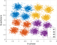
(a) Baseline-1, $\hat{\alpha}=0.5$

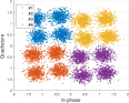
(b) Baseline-2, $\hat{\alpha}=0.5$

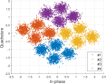
(c) DAE-ZIC, $\hat{\alpha}=0.5$

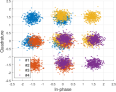
(d) Baseline-1, $\hat{\alpha}=1$

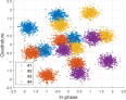
(e) Baseline-2, $\hat{\alpha}=1$

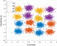
(f) DAE-ZIC, $\hat{\alpha}=1$

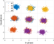
(g) Baseline-1, $\hat{\alpha}=1.5$

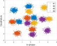
(h) Baseline-2, $\hat{\alpha}=1.5$

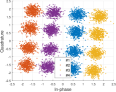
(i) DAE-ZIC, $\hat{\alpha}=1.5$

Figure 4: Constellations of the DAE-ZIC and the two baselines at Rx1 with estimated channels for three values of $\hat{\alpha}$.

TABLE II: The percentage of BER reduction obtained by the DAE-ZIC compared to Baseline-1 and Baseline-2 for different values of $\sigma_{E}^{2}$ and $N_{s}$.

Compared to		Baseline-1		Baseline-2
$N_{s}$		2	3	2	3
$\sigma_{E}^{2}$	$0$	75.77%	44.29%	44.43%	31.50%
	$0.05$	55.40%	38.97%	39.12%	31.43%
	$0.1$	48.83%	35.81%	41.41%	29.24%

We evaluate the performance on two levels of estimation error, $\sigma_{E}^{2}\in\{0.05,0.1\}$. We test the BER over 15500 random channels. The interference intensity $\alpha$ is uniformly generated from $0$ to $3$ with step $0.1$, and SNR is $10$dB. The BER reduction achieved by the proposed DAE-ZIC compared to the baseline methods is shown in Table II. The DAE-ZIC has a remarkable improvement in BER in all interference intensity and estimation error levels. The main improvement of the proposed DAE-ZIC comes from that it designs new, non-overlapping constellations based on the interference intensity.

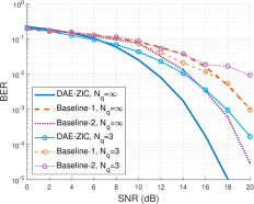
(a) ${M}_{1}={M}_{2}=4$, $\alpha=0.5$

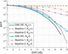
(b) ${M}_{1}={M}_{2}=4$, $\alpha=1$

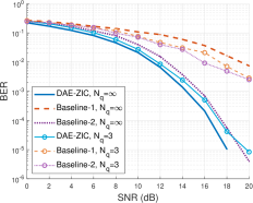
(c) ${M}_{1}={M}_{2}=4$, $\alpha=1.5$

Figure 5: The maximum (worst) BER between the two users (Rx1 and Rx2) versus SNR with and without quantization error.

IV-B CSI with Feedback Quantization

When channel estimation is perfect, the BER performance with feedback quantization (with ${N_{q}=3}$) and without quantization (${N_{q}=\infty}$) is shown in Fig. 5. The DAE-ZIC outperforms the baselines with and without feedback quantization. It is seen that the quantization increases the BER of all methods. However, the performance degradation of the DAE-ZIC is much less than the other two methods. Especially, for $\alpha=1$ and $\alpha=1.5$), where the interference is strong, the DAE-ZIC outperform other methods by over two orders of magnitude when $N_{q}=3$ and $\rm SNR=20$dB. Interestingly, Baseline-1 performs better for $N_{q}=3$ compared to $N_{q}=\infty$. The reason is that quantization of the angles introduces an unintended rotation on Tx2 constellation, unintentionally acting like Baseline-2. This then reduces the constellation overlapping and thus brings a better BER.

With high interference intensities, i.e, $\alpha=1$ and $\alpha=1.5$, the BER of the DAE-ZIC with quantization ($N_{q}=3$) is only slightly degraded compared to the un-quantized case ($N_{q}=\infty$). This is because, while Txs receive the quantized CSI, Rx1 knows CSI before and after quantization. Then, it can to some extent correct the imperfectness in transmitters. Therefore, there is no dramatic degradation for the DAE-ZICs. On the other hand, Baseline-2 is more sensitive to the quantization error and thus a big gap of the BER happens between $N_{q}=\infty$ and $N_{q}=3$. The reason is that Baseline-2 only rotates the constellation in Tx2, which highly depends on the phase shifted by the channels.

V Conclusion

A DAE-based constellation design for the two-user ZIC in the presence of channel estimation error and quantization error has been proposed. The DAE-ZIC minimizes the BER by jointly designing transmit and receive DAEs and optimizing them. A normalization layer is designed to meet the average power constraint. The DAE-ZIC results in more efficient symbols to achieve a lower BER. BER simulations verify the effectiveness of the proposed structure. Our simulation results demonstrate the effectiveness of the proposed structure, and a comparison with two baseline models shows that the DAE-ZIC significantly outperforms both.

References

- [1] A. Carleial, “A case where interference does not reduce capacity (corresp.),” IEEE Trans. Inf. Theory, vol. 21, no. 5, pp. 569–570, 1975.
- [2] T. Han and K. Kobayashi, “A new achievable rate region for the interference channel,” IEEE Trans. Inf. Theory, vol. 27, no. 1, pp. 49–60, 1981.
- [3] R. H. Etkin, D. N. Tse, and H. Wang, “Gaussian interference channel capacity to within one bit,” IEEE Trans. Inf. Theory, vol. 54, no. 12, pp. 5534–5562, 2008.
- [4] A. S. Motahari and A. K. Khandani, “Capacity bounds for the Gaussian interference channel,” IEEE Trans. Inf. Theory, vol. 55, no. 2, pp. 620–643, 2009.
- [5] Y. Wu, C. Xiao, X. Gao, J. D. Matyjas, and Z. Ding, “Linear precoder design for MIMO interference channels with finite-alphabet signaling,” IEEE Trans. Commun., vol. 61, no. 9, pp. 3766–3780, 2013.
- [6] G. Foschini, R. Gitlin, and S. Weinstein, “Optimization of two-dimensional signal constellations in the presence of Gaussian noise,” IEEE Trans. Commun., vol. 22, no. 1, pp. 28–38, 1974.
- [7] A. J. Goldsmith and S.-G. Chua, “Variable-rate variable-power MQAM for fading channels,” IEEE Trans. Commun., vol. 45, no. 10, pp. 1218–1230, 1997.
- [8] M. F. Barsoum, C. Jones, and M. Fitz, “Constellation design via capacity maximization,” in Proc. IEEE Int. Symp. Inf. Theory, pp. 1821–1825, 2007.
- [9] M. Vaezi and H. V. Poor, “Simplified Han-Kobayashi region for one-sided and mixed Gaussian interference channels,” in Proc. IEEE Int. Conf. Commun. (ICC), pp. 1–6, 2016.
- [10] F. Knabe and A. Sezgin, “Achievable rates in two-user interference channels with finite inputs and (very) strong interference,” in Proc. IEEE Asilomar Conf. Signals Syst. Comput. (ACSSC), pp. 2050–2054, 2010.
- [11] A. Ganesan and B. S. Rajan, “Two-user Gaussian interference channel with finite constellation input and FDMA,” IEEE Trans. Wirel. Commun., vol. 11, no. 7, pp. 2496–2507, 2012.
- [12] T. O’Shea and J. Hoydis, “An introduction to deep learning for the physical layer,” IEEE Trans. Cogn. Commun. Netw., vol. 3, no. 4, pp. 563–575, 2017.
- [13] X. Zhang, M. Vaezi, and T. J. O’Shea, “SVD-embedded deep autoencoder for MIMO communications,” in Proc. IEEE Int. Conf. Commun. (ICC), pp. 1–6, 2022.
- [14] J. Song, C. Häger, J. Schröder, T. O’Shea, and H. Wymeersch, “Benchmarking end-to-end learning of MIMO physical-layer communication,” in Proc. IEEE Glob. Commun. Conf. (GLOBECOM), pp. 1–6, 2020.
- [15] T. Erpek, T. J. O’Shea, and T. C. Clancy, “Learning a physical layer scheme for the MIMO interference channel,” in Proc. IEEE Int. Conf. Commun. (ICC), pp. 1–5, 2018.
- [16] D. Wu, M. Nekovee, and Y. Wang, “Deep learning-based autoencoder for M-user wireless interference channel physical layer design,” IEEE Access, vol. 8, pp. 174679–174691, 2020.
- [17] Y. Chen and C. Tellambura, “Performance analysis of maximum ratio transmission with imperfect channel estimation,” IEEE Commun. Lett., vol. 9, no. 4, pp. 322–324, 2005.
- [18] G. Kramer, “Review of rate regions for interference channels,” in Proc. IEEE Int. Zurich Seminar Commun. (IZSC), pp. 162–165, 2004.
- [19] X. Zhang and M. Vaezi, “Deep autoencoder-based Z-interference channels,” in Proc. IEEE Wireless Commun. Netw. Conf. (WCNC), 2023.