Rediscovery of CNN’s Versatility
for Text-based Encoding of Raw Electronic Health Records

Abstract

Making the most use of abundant information in electronic health records (EHR) is rapidly becoming an important topic in the medical domain. Recent work presented a promising framework that embeds entire features in raw EHR data regardless of its form and medical code standards. The framework, however, only focuses on encoding EHR with minimal preprocessing and fails to consider how to learn efficient EHR representation in terms of computation and memory usage. In this paper, we search for a versatile encoder not only reducing the large data into a manageable size but also well preserving the core information of patients to perform diverse clinical tasks. We found that hierarchically structured Convolutional Neural Network (CNN) often outperforms the state-of-the-art model on diverse tasks such as reconstruction, prediction, and generation, even with fewer parameters and less training time. Moreover, it turns out that making use of the inherent hierarchy of EHR data can boost the performance of any kind of backbone models and clinical tasks performed. Through extensive experiments, we present concrete evidence to generalize our research findings into real-world practice. We give a clear guideline on building the encoder based on the research findings captured while exploring numerous settings.

Data and Code Availability

This paper uses the MIMIC-III and eICU datasets, which are available on PhysioNet repository (Johnson et al., 2016b; Pollard et al., 2018). The source code is available at the Github repository.

Institutional Review Board (IRB)

This research does not require IRB approval.

1 Introduction

The widespread introduction of electronic health record (EHR) systems brings tremendous opportunities to apply a data-driven approach to the healthcare domain. Through EHR systems, millions of patients’ data are now collected in a systematic manner across diverse healthcare institutions. Using this rapidly growing EHR dataset, many researchers have found applications such as predicting clinical outcomes, learning representations of cohorts to get medical insights, and synthesizing clinical data.

To perform EHR-related tasks, conventional frameworks employed various encoding architectures such as Recurrent Neural Networks Lipton et al. (2015); Choi et al. (2015); Rajkomar et al. (2018), Convolutional Neural Networks Miotto et al. (2016); Nguyen et al. (2016); Landi et al. (2020), and Transformer-based models Yoon et al. (2022); Choi et al. (2019); Shang et al. (2019); Rasmy et al. (2020); Li et al. (2020); Song et al. (2018). Despite the diversity of proposed works, all these attempts have clear limitations in that they are applicable exclusively to their own EHR system. For example, they cannot use both MIMIC-III Johnson et al. (2016b, a); Goldberger et al. (2000) and eICU Pollard et al. (2018); Johnson et al. (2019) datasets together for training, unless involving manual harmonization of incompatible features. In addition, inherent disparities in the standards of medical codes and database schemas prevent data from being sourced from multiple healthcare institutions. None of previous works thus can fully utilize information in multiple diverse EHR systems.

A recent work Hur et al. (2021, 2022) presented a text-based encoding approach to address this conventional limitation. Specifically, Hur et al. (2022) proposed a universal framework that can embed entire features in raw EHR data regardless of its schema and medical code standards. Moreover, the framework showed comparable, if not better, performance on various tasks, even without relying on domain knowledge-based preprocessing. However, it comes at a steep price of the embedded data having tens to hundreds of times larger in size than existing methods, even if it covers only a few hours of medical trajectory of a patient in hospital. Therefore, a structure that efficiently extracts the core information from the large input is needed.

In this study, we search for a versatile model architecture to encode the raw EHR input into a low-dimensional space under the universal text-based encoding framework for diverse tasks such as reconstruction (i.e., autoencoding), prediction, and generation. Throughout the paper, we make the following contributions:

• To the best of our knowledge, this is the first work to search for a versatile encoder not only reduces the large raw EHR into a manageable size but also preserves patients’ core information to perform diverse clinical tasks.

• We conduct extensive experiments with multiple variables to tune model architectures and various clinical tasks (i.e., reconstruction, prediction, generation). Furthermore, by experimenting with two representative datasets in the EHR domain (i.e., MIMIC-III, eICU), we present concrete evidence for generalizing our research findings to a wide variety of EHR systems. We capture the core tendencies while exploring these numerous settings and systematically summarize the findings to give a clear guideline on building the encoder.

• The encoder that we found is widely applicable in real-world practice. Even with fewer parameters and less training time, a hierarchically structured CNN often outperforms the state-of-the-art model on widely accepted tasks in the field.

2 Related work

Feature-selection-based encoder for EHR

Many researchers have applied a data-driven approach to the healthcare domain. By making use of EHR datasets, they predict medical outcomes, learn the representation of patients for various downstream tasks, and synthesize medical data. To perform the clinical tasks, they employed various encoding backbones such as Recurrent Neural Network Lipton et al. (2015); Choi et al. (2015); Rajkomar et al. (2018), Convolutional Neural Network Miotto et al. (2016); Nguyen et al. (2016); Landi et al. (2020), and Transformer Yoon et al. (2022); Choi et al. (2019); Shang et al. (2019); Rasmy et al. (2020); Li et al. (2020); Song et al. (2018). However, all such works have invested a lot in preprocessing the raw EHR for standardizing the EHR schema, or feature engineering specifically for the given task. This is a clear limitation in that extensive human labor and clinical domain knowledge are required to produce satisfactory model performance.

Universal Healthcare Predictive Framework

Recently, Hur et al. (2022) presented UniHPF, a universal framework that can embed entire features of raw EHR regardless of schema and medical code standard used in the database. Specifically, UniHPF views EHR data as pure text and flattened the EHR tables (e.g. prescriptions, lab results) to feed them to Transformer-based text encoders. This text-based approach showed comparable if not better performance compared to conventional approaches on various predictive tasks, even without relying on medical domain knowledge. Ironically, because it can handle raw EHR data without any preprocessing or feature selection, UniHPF generates extremely long embedded data, given how it encodes entire EHR data in a text-encoding fashion . This imposes strong computational limits on the framework and necessitates an additional module for compressing the embedded data to a smaller size.

3 Method

fig:mainfigure [Illustration of EHR tables and patient representation]

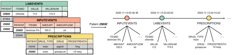
Figure 1: EHR structure and encoder framework.

[Encoder framework and examples of hierarchical input $\textbf{x}_{hi}$ and flattened input $\textbf{x}_{fl}$]

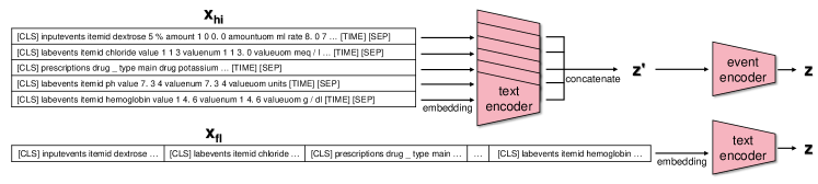
In order to search for a versatile encoder for raw text-based EHR, we examine different encoder designs. In subsec:EHRSerial, we first show how raw tabular EHR is converted into natural text, following the embedding strategy of UniHPF. In subsec:EncodingFramework, we construct both hierarchical and flattened encoder structures to confirm the effectiveness of reflecting EHR hierarchy. Also, two highly scalable model classes of CNN and Transformer are considered as backbone models .

As shown in fig:Pipeline, we evaluate the significance of the encoder in downstream tasks such as prediction, reconstruction, and generation. Accordingly, we present decoder architectures for reconstruction and generation in subsec:TaskSpecificModels and explanations for other task-specific models (e.g., classifier) in sec:expdesign.

3.1 EHR serialization

EHR structure

Once a patient is admitted to the intensive care unit (ICU), a series of medical events occur during the ICU stay. Each event is recorded in one of several tables, such as prescription, diagnosis, lab events and input events in the hospital database. Each table consists of multiple rows (e.g., lab events), which in turn consist of multiple columns representing different feature variables (e.g., lab date, lab name, lab value). The type of cell values can be categorized as textual, numeric, and itemized values (e.g., lab test ID) that can be textualized using a description from the definition table. fig:EHRstructure provides an overview of EHR structure.

EHR serialization

In order to construct the input data, we first extract each patient’s records from the multiple tables in the hospital database and sort all events chronologically. Following the UniHPF-strategy, we formulate patient representation as

$$\textbf{x}=f(\texttt{column name}\otimes g(\texttt{cell})\otimes\texttt{timegap})$$

where $f$ is a tokenizer, $g$ is a mapping function that converts the type of cell value to text, $\otimes$ is the concatenate function, and timegap represents the quantized time interval between consecutive events. In detail, $g$ converts an itemized value to a corresponding free text description (e.g., lab test ID 51385 to “Atypical Lymphocyte”) and numeric values to text separated by space (e.g., 123.1 to “1 2 3 . 1”). For $f$, resulting texts are tokenized into the sub-word level. In this way, with minimal pre-processing, we construct the patient representation x as a sequence of discrete tokens.

In addition, as shown in fig:EHRstructure, the patient representation has two levels of hierarchy; event and feature levels. Specifically, it is described by a sequence of events where each event consists of multiple features. Making use of this hierarchical relationship between events and their corresponding features, we define hierarchical input $\textbf{x}_{hi}\in\mathbb{R}^{n_{e}\times n_{t/e}}$, and flattened input $\textbf{x}_{fl}\in\mathbb{R}^{n_{t}}$, where $n_{e}$, $n_{t/e}$, and $n_{t}$ are, respectively, the number of events, the number of text tokens per event, and the number of flattened text tokens.

Note that padding and truncation approaches are used to make fixed $n_{e}$, $n_{t/e}$, and $n_{t}$. Since $\textbf{x}_{fl}$ is an unfolded version of $\textbf{x}_{hi}$ with padding removed and events concatenated, $n_{t}$ is less than $n_{e}\times n_{t/e}$ although $\textbf{x}_{fl}$ and $\textbf{x}_{hi}$ contain exactly the same amount of information. Examples of $\textbf{x}_{hi}$ and $\textbf{x}_{fl}$ are shown on the left part in fig:EncoderStructure.

3.2 Encoding framework

Embedding

Before feeding the input sequence to an encoder, we embed tokens according to the UniHPF embedding approach. Details are specified in apd:AdditionalEmbedding. We denote the hierarchical input embedding by $\textbf{E}_{hi}=\mathtt{Emb}(\textbf{x}_{hi})\in\mathbb{R}^{n_{e}\times n_{t/e}\times d}$, and the flattened input embedding by $\textbf{E}_{fl}=\mathtt{Emb}(\textbf{x}_{fl})\in\mathbb{R}^{n_{t}\times d}$, where $d$ is the token embedding dimension.

Encoder

To encode $\textbf{E}_{hi}$ and $\mathbf{E}_{fl}$ into latent vector z, we construct $\mathtt{Enc}_{struc}$ reflecting the input structure. fig:EncoderStructure summarizes the overall encoding process.

For hierarchical embedding $\textbf{E}_{hi}$, we use a two-stage encoder $\mathtt{Enc}_{hi}$ consisting of a text encoder $\mathtt{Enc}^{t}$ for token embedding within an event, followed by an event encoder $\mathtt{Enc}^{e}$ for aggregating and compressing encoded events $\textbf{z}^{\prime}$ into z. Specifically, $\mathtt{Enc}^{t}$ takes per-event token embeddings $\{\textbf{e}_{hi}^{i}\}_{i=1}^{n_{e}}\subset\mathbb{R}^{n_{t/e}\times d}$ as input and produces $\textbf{z}^{\prime}\in\mathbb{R}^{n_{e}\times d^{\prime}}$ with the following operation:

$$\textbf{z}^{\prime}=\mathtt{Concat}(\mathtt{Flatten}([\mathtt{Enc}^{t}(\textbf{e}_{hi}^{1}),...,\mathtt{Enc}^{t}(\textbf{e}_{hi}^{n_{e}})]))$$

where $\mathtt{Flatten}$ is an element-wise operation that expands each $\mathtt{Enc}^{t}(\textbf{e}_{hi}^{i})$ into a 1D vector with $d^{\prime}$ dimension and $\mathtt{Concat}$ is a function that concatenates events in a chronological order. Note that all $\mathtt{Enc}^{t}$ are shared across events. Afterwards, $\mathtt{Enc}^{e}$ compresses $\textbf{z}^{\prime}$ into a latent vector $\textbf{z}\in\mathbb{R}^{t\times c}$ where $t$ and $c$ are the desired temporal and channel dimension, respectively. Such a two-stage process gives the encoder explicit information about the hierarchical structure between events and their features.

For flattened embedding $\textbf{E}_{fl}$, we use an one-stage encoder $\mathtt{Enc}_{fl}$ consisting only of $\mathtt{Enc}^{t}$, which directly compress $\textbf{E}_{fl}$ into z.

3.3 Encoding schemes

In this section, we describe how the input embedding $\textbf{E}_{hi}$ or $\textbf{E}_{fl}$ is compressed into z of a desired dimension. Note that the encoding strategy is shared for both $\mathtt{Enc}^{t}$ and $\mathtt{Enc}^{e}$. Therefore, we can generalize the input and output of each encoder as $\textbf{E}_{input}\in\mathbb{R}^{n\times d}$ with $n$ sequence length and $d$ dimension, and $\textbf{E}_{output}\in\mathbb{R}^{n^{\prime}\times d^{\prime}}$ where $n^{\prime}$ and $d^{\prime}$ denote the desired length and hidden dimension.

We consider using CNN and Transformer as the backbone of the encoder and develop a custom encoding scheme for each of them. We examine several Transformer-based encoding schemes summarized in apd:TransfEncoding and decide on the encoding strategy for each backbone. alg:CNNlayernum and 3 summarize the CNN encoding scheme, while alg:Transformer summarizes Transformer encoding scheme. Specific examples of each algorithm are provided in tab:algCNN and tab:algTransf.

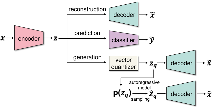
Figure 2: Overall pipeline. We search for a versatile encoder design and validate it in three downstream tasks: reconstruction, prediction, and generation.

3.4 Decoder

We employ CNN-based and Transformer-based decoder architectures for the reconstruction and generation tasks (shown in fig:Pipeline).

The CNN-based decoder is designed with a symmetric structure of the CNN-based encoder. Specifically, while the encoder layers either compress the dimension in half or leave it unchanged, the decoder layers inversely expand the dimension by two or leave it unchanged, respectively.

For the Transformer-based decoder, we reconstruct the original input x by using cross attention between the latent vector z and a learnable placeholder embedding with the identical length of x. Specifically, the placeholder embeddings are randomly initialized at first, and while passing through each layer of the decoder, the embeddings are decompressed at the channel level with cross attention applied. As shown in the decoder of fig:transformerdecoder, the decoder block consists of a Transformer decoder layer in which cross-attention is applied and a linear layer for channel increase. Between the encoder and decoder, we add linear layers in order to match the latent and placeholder dimensions before applying cross attention. This is because the placeholder embedding dimension is increased with each decoder layer. An exploration of various Transformer-based decoder architectures can be found in apd:TransfDec.

4 Experiments

4.1 Dataset description

Source data

We experimented with two representative datasets in the EHR domain; MIMIC-III and eICU. The MIMIC-III dataset comprises deidentified clinical data from more than 40,000 patients admitted to the ICU of Beth Israel Deaconess Medical Center. The eICU is populated with data from around 140,000 patients who were admitted to a combination of many critical care units throughout the continental United States. To fully represent patients’ medical trajectories, the datasets contain many medical events, such as laboratory test, prescriptions, and input events (e.g., fluid injections) with temporal information. In accordance with the UniHPF configuration, we employed solely three tables from both datasets - laboratory test, prescriptions, and input events.

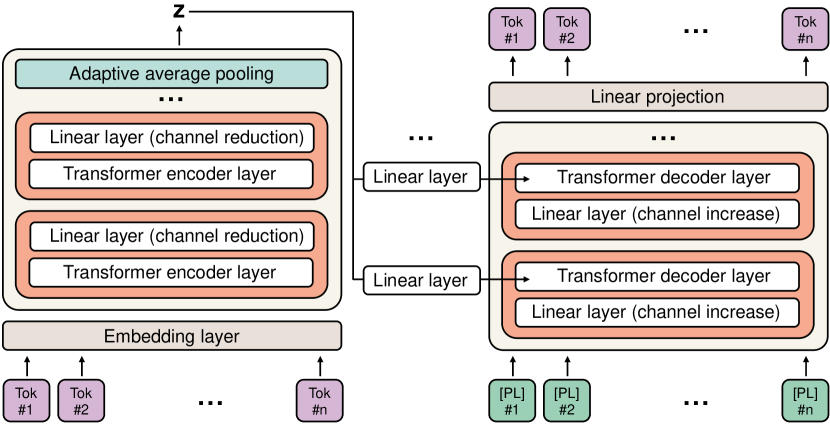
Figure 3: Proposed Transformer-based encoder and decoder architecture.

Cohort definition

To build cohorts of patients from MIMIC-III and eICU databases, we follow the criteria on which the universal framework Hur et al. (2022) is based. We retrieve records of patients over 18 years old who stayed in the ICU for over 24 hours. We filter out ICU stays with less than five medical events and use the first 12 hours of events of the first ICU stay for each hospital stay. For both datasets, we divide patients into separate train, validation, and test sets with a ratio of 8:1:1.

4.2 Experimental design and model

We perform three downstream tasks: reconstruction, prediction, and generation. For each downstream task, we explore multiple settings for the encoder $\mathtt{Enc}_{struc}$ (or additionally decoder $\mathtt{Dec}_{struc}$), where $struc\in\{hi,fl\}$. We use the same $struc$ for both $\mathtt{Enc}_{struc}$ and $\mathtt{Dec}_{struc}$. Their backbone can either be CNN or Transformer, denoted by $C$ and $T$, respectively.

Reconstruction task

In order to evaluate the efficacy of the encoder in preserving patient information, we build an autoencoder as follows:

$$\mathbf{\tilde{x}}=\mathtt{Dec}_{struc}(\mathtt{Enc}_{struc}(\mathbf{x}))$$

We train the autoencoder with a cross-entropy loss between $\mathbf{x}$ and $\mathbf{\tilde{x}}$. We experimented $(\mathtt{Enc}_{struc},\mathtt{Dec}_{struc})$ on $(C,C),(T,C)\text{ and }(T,T)$ for $hi$ and $fl$. We evaluate the reconstruction performance via token-level accuracy, the ratio of correct tokens to the total number of tokens.

Prediction task

To perform clinical outcome prediction, we formulate the task as binary, multi-class or multi-label classification:

$$\tilde{\textbf{y}}=\mathtt{Classifier}(\mathtt{Enc}_{struc}(\mathbf{x}))$$

The encoder and classifier are trained with the binary cross-entropy loss (cross-entropy loss for multi-class) between the predicted probabilities $\tilde{\textbf{y}}$ and the true label y. For $\mathtt{Classifier}$, we use Transformer due to its permutation invariant nature, rather than a purely MLP-based classifier. After linearly projecting x into z, we pass z through the Transformer layers. The output is then averaged and linearly mapped to generate logits for each class. We adopted six clinically meaningful prediction tasks following Hur et al. (2022); Diagnosis, Mortality, Final acuity Imminent Discharge, Length-Of-Stay for cases of three and seven days. Further details of each clinical task are provided in the apd:DefClinicTask. We evaluated all prediction tasks in terms of AUROC.

Generation task

For the unconditional synthesis of textualized EHR x, autoregressive modeling of x is challenging due to the high modeling capacity and memory inefficiency required by the considerable sequence length of UniHPF syntax. Therefore, we use the VQ-VAE Van Den Oord et al. (2017) approach to model the discrete latent space autoregressively. The VQ-VAE consists of $\mathtt{Enc}_{struc}$, $\mathtt{Dec}_{struc}$, a vector quantization layer $\mathtt{VQ}$ and a learnable codebook, formulated as follows:

$$\textbf{z}_{q} =\mathtt{VQ}(\mathtt{Enc}_{struc}(\textbf{x})),\ \tilde{\textbf{x}}=\mathtt{Dec}_{struc}(\textbf{z}_{q})$$

$$\hat{\textbf{x}} =\mathtt{Dec}_{struc}(\hat{\textbf{z}}_{q})\ \text{where}\ \hat{\textbf{z}}_{q}\sim p(\textbf{z}_{q})$$

where $\mathtt{VQ}$ maps each vector $\textbf{z}=\mathtt{Enc}_{struc}(\textbf{x})$ into $\textbf{z}_{q}$ with the nearest code. The VQ-VAE is trained in two steps. First, $\mathtt{Enc}_{struc}$, $\mathtt{Dec}_{struc}$, and the codebook are trained simultaneously to minimize the distance between x and $\tilde{\textbf{x}}$ and the distance between z and $\textbf{z}_{q}$. Second, the Transformer-based autoregressive model is trained to learn the prior distribution over the discrete latent space $p(\textbf{z}_{q})$. Then the sampled latent code sequence $\hat{\textbf{z}}_{q}$ is passed into the decoder to synthesize $\hat{\textbf{x}}$. Further details of training VQ-VAE are in apd:VQVAE. We conduct experiments on $(C,C)$, $(T,C)$ and $(T,T)$ for $(\mathtt{Enc}_{hi},\mathtt{Dec}_{hi})$.

We assess the quality of synthetic data quantitatively, qualitatively, and from a privacy perspective.

We propose a metric to measure the preservation of table syntax and semantic consistency by comparing triples (table, column name, cell) in generated data with real data. For example, the lab ID should be on a lab table, not a prescription table. On a per-event or per-sample basis, we compute RCE (ratio of correct events to total events), RUE (ratio of correct unique events to total unique events), and RCS (ratio of correct samples to total samples). Specifics regarding the evaluation algorithm and scoring metrics are listed in apd:SyntheticDataScoring.

To qualitatively compare the distribution of original and synthetic data, we used t-SNE to visualize latent vectors in a two-dimensional space.

In addition, for the privacy evaluation, we conducted a membership inference attack Shokri et al. (2017), and the task definition and results are shown in apd:MI.

4.3 Implementation details

For the CNN-based encoder (alg:CNNlayernum and 3), we employed a scheme that compresses the dimension as desired by combining two types of kernels, one with a kernel size of 5, a stride of 2, and a padding size of 2, and the other with a kernel size of 1 and a stride of 1 and no padding.

For the Transformer-based encoder (alg:Transformer), we use four Transformer layers for $\mathtt{Enc}_{hi}$ and four Performer Choromanski et al. (2020) layers for $\mathtt{Enc}_{fl}$, in which all layers in both $\mathtt{Enc}_{hi}$ and $\mathtt{Enc}_{fl}$ use 4 attention heads.

We use 2 Transformer layers with 4 heads and a hidden dimension of 128 for the $\mathtt{Classifier}$. As for the Transformer-based autoregressive model used for generation, we utilize 4 Transformer layers with 4 heads and a hidden dimension of 256. The Adam optimizer Kingma and Ba (2014), along with a learning rate of 5e-4 (or 5e-5 for models that failed to train), is employed for the optimization process. Additionally, we select different batch sizes of 16, 64, and 32 for reconstruction, prediction, and generation, respectively. Experiments are conducted with different random seed values, with three seeds for reconstruction and prediction, and two seeds for the generation.

4.4 Searching range

For input embeddings $\textbf{E}_{hi}\in\mathbb{R}^{n_{e}\times n_{t/e}\times d}$ and $\textbf{E}_{fl}\in\mathbb{R}^{n_{t}\times d}$, we employ $n_{e}=256$, $n_{t/e}=128$ for $\textbf{E}_{hi}$, and $n_{t}=8192$ for $\textbf{E}_{fl}$. The embedding layer $\mathtt{Emb}$ has a fixed dimension $d=256$. For the compressed latent vector $\textbf{z}\in\mathbb{R}^{t\times c}$ of $\textbf{E}_{hi}$ and $\textbf{E}_{fl}$, we define the latent dimension $l=t\times c$.

For prediction and reconstruction tasks, we explore its size starting from $l$ = 256 and double it up until $l$ = 4096. For each $l$, represented as $2^{2i-1}$ or $2^{2i}$, we search five possible cases of $t$ from $2^{i-2}$ to $2^{i+2}$ by increasing $i$. (e.g., For the latent vector z having $l=2048=2^{2*6-1}$, we search $t$ from $2^{4}$ to $2^{8}$).

However, for the generation task, we use a less compressed searching range of $l$, starting from 4096 up to 32768. This is because the first stage in VQVAE can be viewed as conducting reconstruction along with vector quantization, in which additional information loss is inevitable.

Compression rate, indicating how many times z is smaller than $\textbf{E}_{hi}$ or $\textbf{E}_{fl}$, can be calculated by $\frac{n_{e}\times n_{t/e}\times d}{l}$ and $\frac{n_{t}\times d}{l}$, respectively. (e.g., if z has a shape of $(256,8)$ in hierarchical case, the compression rate is ${\times}4096=\frac{256\times 128\times 256}{2048}$). Consequently, $\mathtt{Enc}_{hi}$ has a compression rate ranging from 2048 to 32768, while $\mathtt{Enc}_{fl}$ has a lower rate ranging from 512 to 8192.

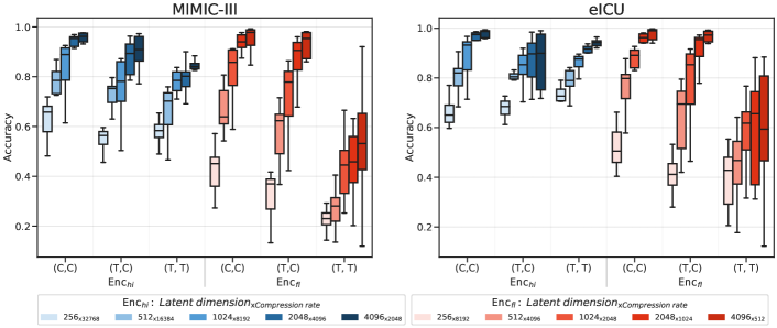
fig:comparison_recon_mimic_eicu [Reconstruction performances arranged by the latent dimension $l$] [Reconstruction performances arranged by the temporal dimension $t$]

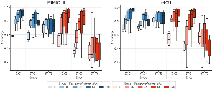
Figure 4: Comparison of reconstruction performance for both MIMIC-III (left) and eICU (right) datasets.

fig:comparison_pred_mimic_eicu [Prediction performances arranged by the latent dimension $l$]

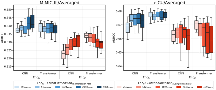
Figure 5: Comparison of prediction performance for both MIMIC-III (left) and eICU (right) datasets.

[Prediction performances arranged by the temporal dimension $t$]

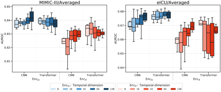
5 Result

We conducted extensive experiments on building $\mathtt{Enc}_{struc}$ for the above reconstruction, prediction, and generation tasks. Specifically, we experiment on different types of backbone models, both $hi$ and $fl$ structures, and various combinations of ($t$, $c$) of latent vector z $\in\mathbb{R}^{t\times c}$. When comparing performances using box plots, it is important to consider both the mean and best performances respectively represented by the box’s position and the upper whisker, as each box contains several model variants of the same latent dimension or temporal dimension.

5.1 Reconstruction

For the reconstruction task for MIMIC-III and eICU datasets, CNN outperforms Transformer when used as both the encoder and a decoder. recon_summary_latent shows the reconstruction performances of autoencoders $(C,C)$, $(T,T)$, and $(T,C)$ at the same latent dimension $l$. We evaluated each backbone as an encoder by comparing models with the different encoders but with the same decoder and vice versa for the decoder case.

Results in recon_summary_latent show that CNN is a better encoder compared to Transformer, as $(C,C)$ shows higher performance compared to $(T,C)$ for both $hi$ and $fl$ structures. When compared in the same manner, CNN as a decoder showed a far better performance than Transformer with a much wider margin than the encoder case. The conclusion that CNN is better in both aspects is reinforced by the fact that the autoencoder composed solely of CNN performs better than that of Transformers.

Finding

Our experiment results show that EHR as a time series dataset has inherent temporal locality; each medical event contained in EHR is mainly correlated with events that happened in a short period. Specifically, the reconstruction results with CNN, having a local receptive field, outperform that of Transformer, which has a global receptive field. Moreover, as depicted in apd:LocalEHR, Transformer mainly attends temporally proximal events represented by the elements near the diagonal line, which shows an entirely different pattern in the case of prediction. Lastly, by rearranging the results with temporal dimension $t$ as shown in recon_summary_temporal, CNN performs clearly better as $t$ increases, while the performance of Transformer either remains stagnant or decreases. Thus, in order to preserve patient information with minimal loss, it is better to keep more temporal information even within the same latent dimension.

5.2 Prediction

For the prediction tasks, the CNN-based encoder shows comparable performance to the Transformer-based encoder in the hierarchical setting. pred_summary illustrates the averaged AUROC performance of the six prediction tasks for each model architecture. As the four models share the same classifier, we compare the results based on different encoder settings. Specific results for each task are reported in apd:Pred6Tasks. For the $hi$ setting, the CNN-based encoder shows comparable performance to Transformer, whereas for the $fl$ setting, CNN shows lower performance. Such results imply that explicit information on EHR hierarchy is more effective for the CNN compared to the Transformer in predictive tasks.

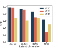
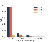
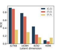
fig:quan_eval_mimic_eicu [MIMIC-III/RCE][MIMIC-III/RCS][eICU/RCE] [eICU/RCS]

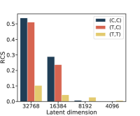
Figure 6: Quantitative evaluation on MIMIC-III and eICU datasets. RCE and RCS represent the ratio of correct events to total events and the ratio of correct samples to total samples, respectively.

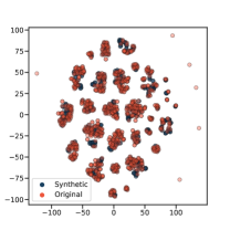
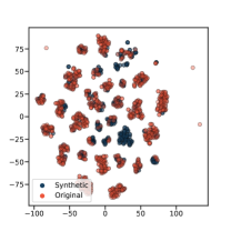
fig:tsne_mimic [(C,C)][(T,C)] [(T,T)]

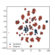
Figure 7: t-SNE visualization on latent space on MIMIC-III dataset.

Finding

For the CNN-based encoder, both reconstruction and prediction tasks showed a significant positive correlation. As shown in apd:pca, the CNN-based encoder learns similar latent representations for reconstruction and prediction. Moreover, as shown in pred_summary_temporal, keeping more temporal information by increasing $t$ improves the predictive performance, even within the same $l$. By increasing $t$, we can thus enhance the CNN-based encoder in both aspects simultaneously; the higher performance for both reconstruction and prediction tasks.

5.3 Generation

Quantitative evaluation

As shown in fig:scores, we report the results of proposed metrics according to the different $(\mathtt{Enc}_{hi},\mathtt{Dec}_{hi})$ combinations, and latent dimensions. High RCE indicates that each generated event follows the table structure while maintaining the semantic consistency of input. The RCS, a stricter measure, denotes the amount of synthetic patient data readily available. In the case of latent dimension 32768, $(C,C)$ and $(T,C)$ show comparable performance. However, as the compression rate increases, the performance gap between $(C,C)$ and $(T,C)$ is enlarged, with $(C,C)$ showing superior performance. Such results indicate that the CNN-based encoder effectively preserves patient information despite a high compression rate. $(T,T)$, on the other hand, generally shows the lowest performance compared to both $(C,C)$ and $(T,C)$. We also report RUE on the apd:RUE.

Qualitative evaluation

We conduct t-SNE on the encoded latent $\textbf{z}\in\mathbb{R}^{32768}$ of $(C,C)$, $(T,C)$ and $(T,T)$ for both the original and synthetic data, as shown in fig:tsne. The distributions of both the original and synthetic data surprisingly form in multiple clusters with some outliers. For the case of $(C,C)$, although the synthetic data distribution does not cover all outliers, it shows clusterings in similar regions to the original. On the other hand, the synthetic data of $(T,C)$ and especially $(T,T)$ also form condensed clusters that resemble those of the original data. However, some clusters do not contain any original data clusters. Such results show that compared to the Transformer-based encoder, the CNN-based encoder better encodes the input with similar distributions to the original data. We also included t-SNE visualization results according to perplexity values in apd:tsne_ppl.

Furthermore, the poor performance of membership inference attack in apd:MI showed a low possibility of privacy leakage.

5.4 Structure

We compared the hierarchical structure to the flattened one to measure the effect with all the other variables controlled. In recon_summary and pred_summary, the blue histograms are positioned higher than the red ones, indicating that hierarchically structuring the model led to higher performance across tasks and backbone models. Using the inherent hierarchy of the EHR system can boost the model’s performance.

5.5 Time and Parameter Efficiency

We compare the resource consumption of each model in our experiments. fig:efficiency illustrates the parameters-performance, FLOPs-performance, and time-performance curves for the models performing the reconstruction task. We only consider the encoder without the rest of the model for the number of parameters and time consumed for training. Compared to the Transformer-based models, the results of the CNN-based models are located in the upper left part for all 8, 8 and 8. Thus, CNN is a better backbone for building an encoder than Transformer, even with notably fewer parameters and lower computational cost.

[Model Size vs. Performance]

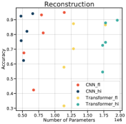
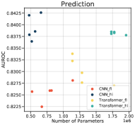
[FLOPs vs. Performance]

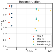
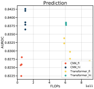
[Training time vs. Performance]

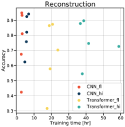
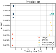
Figure 8: Reconstruction (left) and prediction (right) performances on MIMIC-III relative to the resource (the number of parameters, FLOPs, and training time) consumed. In all figures, CNN having $hi$ structure is located in the upper left corner; it shows better performance with lower cost than the others. For each model, we grouped variants based on $l=t\times c$ and averaged them. As the recipe of building $\mathtt{Enc}_{struc}$ varies by the ratio of $t$ to $c$ even within same $l$, the model size is not strictly proportional to the compression rate.

6 Conclusion

We have searched for a versatile architecture to encode the raw EHR input into a low-dimensional space when the input processed by the universal framework is on a large scale. To the best of our knowledge, this is the first work to search for a versatile encoder not only reducing the large EHR into a manageable size but also well preserving the core information of patients to perform clinical tasks. Even with fewer parameters and less training time, hierarchical CNN outperforms the state-of-the-art model on widely accepted tasks in the field. Moreover, it turns out that making use of the inherent hierarchy of the EHR system can boost the performance of any backbone models and clinical tasks performed. By conducting extensive experiments, we present concrete evidence for generalizing our research findings into real-world practice. We capture the core tendencies while exploring these numerous settings and systematically summarize the findings to give a clear guideline on building the encoder.

We are grateful to Seongsu Bae, Sungjin Park, and Jiyoung Lee for their fruitful comments and inspiration. We acknowledge the support of Google’s TPU Research Cloud (TRC), which provided us with Cloud TPUs to conduct the research. This work was supported by Institute of Information & Communications Technology Planning & Evaluation (IITP) grant (No.2019-0-00075), National Research Foundation of Korea (NRF) grant (NRF-2020H1D3A2A03100945), and the Korea Health Industry Development Institute (KHIDI) grant (No.HI21C1138), funded by the Korea government (MSIT, MOHW).

Appendix A Input Embedding

Before being embedded to the encoder, token sequence x is first mapped to a vector representation based on a learnable lookup table. Next, we add different types of embeddings to the vector representation:

• Token-type embedding adds structural information of table to the vector representation, considering that the input is based on tabular data. The types of added embeddings are [table name], [column name], [column value], [timegap], [start token], [end token], and [pad token].

• Digit-place embedding adds value embeddings for numeric features (e.g. dosage, rate). Since neural tokenizers are notorious for having difficulty in processing numbers, we use Digit-Place Embedding (DPE) to let the models to recognize numbers naturally. DPE first splits the numeric values into digits and assigns each digit to its place value. For example, ”123.1” becomes ”1 2 3 . 1”, and corresponds to “[hundreds], [tens], [units], [decimal point], [tenth]”. For tokens that are not a number or decimal point, we add [non-digit].

• Positional embedding adds a time signal by mapping each position of the sequence to the embedding space. Such embedding is needed for models without recurrence or convolution, such as the Transformer. Thus, we use sinusoidal positional embedding for the Transformer-based encoder.

Appendix B Algorithm for building encoders and examples

For CNN encoding scheme, alg:CNNlayernum and 3 respectively summarize the number of layers by type and the order of layers. To reduce the biased effect on the manifold in low-dimensional space when compressing only one dimension consecutively, we carefully design the order of layers to compress the temporal and channel dimensions alternately. For Transformer, alg:Transformer summarizes encoding scheme.

We provide examples of algorithms for building encoders in tab:algCNN and 2 for some specific cases.

Input: $\mathbf{E}_{input}\in\mathbb{R}^{n\times d},n^{\prime},d^{\prime}$

// $(n^{\prime},d^{\prime}):$ an expected shape of $\mathbf{E}_{output}$

Output: $D_{enc}$

// $L_{n}$ compresses $n$-axis in half

// $L_{d}$ compresses $d$-axis in half

// $L_{nd}$ compresses $n$ and $d$ axes in half

// Determine the number of layers $n_{l}$

$r_{n},r_{d}\leftarrow log_{2}(n/n^{\prime}),log_{2}(d/d^{\prime})$

$n_{l}\leftarrow max(r_{n},r_{d})$

// Decide the number of layers by type

if $r_{n}>r_{d}$ then

       $D_{enc}\leftarrow\{L_{nd}:r_{d},\;L_{n}:n_{l}-r_{d}\}$

      

else if $r_{n}<r_{d}$ then

       $D_{enc}\leftarrow\{L_{nd}:r_{n},\;L_{d}:n_{l}-r_{n}\}$

      

else

       $D_{enc}\leftarrow\{L_{nd}:n_{l}\}$

      

Algorithm 1 CNN encoding scheme: the number of layers by type

Input: $\textbf{E}_{input}\in\mathbb{R}^{n\times d},n^{\prime},d^{\prime},n_{l}$

Output: encoder layers

$(n^{\prime},d^{\prime}):$ an expected shape of $\textbf{E}_{output}$

// adaptive average pooling: $P_{adpt}(\mathbf{E}_{input},n^{\prime})\in\mathbb{R}^{n^{\prime}\times d^{\prime}}$

$r_{c}\leftarrow log_{2}(d/d^{\prime})$

$q\leftarrow r_{d}//n_{l}$

$r\leftarrow r_{d}\%n_{l}$

// Define the encoder layers

set $L_{d_{1}}$ to decrease channel dim by $2^{q+1}$

set $L_{d_{2}}$ to decrease channel dim by $2^{q}$

return $[L_{d_{1}}]*r+[L_{d_{2}}]*(n_{l}-r)+[P_{adpt}]$

Algorithm 2 Transformer encoding scheme

Appendix C Definition of clinical predictive task

1. Diagnosis (Dx) (multi-label): Predict all diagnoses occurred during the entire ICU stay. By following Clinical Classification Software (CCS) for ICD-9-CM criteria, diagnosis codes are classified into 18 categories.

2. Final Acuity (Fi_ac) (multi-class): At the end of the ICU stay, predict where the patient will be discharged among the various places.

3. Imminent Discharge (Im_disch) (multi-class): Predict whether the patient will be discharged within the subsequent prediction window of 48 hours and, if so, where to be discharged.

Input: $D_{enc},n_{l},r_{n},r_{d}$

Output: encoder layers

// $block_{alt}$ compresses $n$ and $d$ axes alternatively

if $L_{n}\in D_{enc}$ then

       $num_{n}^{block}\leftarrow(n_{l}+1)//(r_{d}+1)$

       $num_{n}^{rem}\leftarrow(n_{l}+1)\%(r_{d}+1)$

       $block_{n}\leftarrow[L_{n}]*\text{max}(num_{n}^{block},0)$

       $block_{alt}\leftarrow block_{n}+[L_{nd}]$

       $block_{alt^{\prime}}\leftarrow block_{alt}+[L_{n}]$

       return ($block_{alt})*(r_{d}-num_{n}^{rem})+(block_{alt^{\prime}})*(num_{n}^{rem})+block_{n}$

      

else if $L_{d}\in D_{enc}$ then

       $block_{alt}\leftarrow[L_{nd},L_{d}]$

       if $n_{l}-2(r_{d}-r_{n})+1<0$ then

             $n_{odd}\leftarrow n_{l}\%2$

             return $[L_{d}]*n_{odd}+block_{alt}*r_{n}+[L_{d}]*(n_{l}-2r_{n}-n_{odd})$

            

      

      else

             if $2r_{n}-r_{d}\geq 0$ then

                  $num_{alt}\leftarrow r_{d}-r_{n}$

             else

                  $num_{alt}\leftarrow\text{min}(r_{n},r_{d}//2)$

            

            if $(r_{n}-num_{alt})=r_{d}-2num_{alt}$ then

                  $block_{non-alt}\leftarrow[L_{nd}]*(r_{n}-num_{alt})$

             else

                  $block_{non-alt}\leftarrow[L_{d}]*(r_{d}-2num_{alt})$

             return $block_{non-alt}+block_{alt}*num_{alt}$

            

      

else

       return $[L_{nd}]*n_{l}$

      

Algorithm 3 CNN encoding scheme: the order of layers

1. Mortality (Mort) (binary): Predict whether or not a patient will be discharged with the state “expired” within the prediction window of 48 hours. The discharge state was “expired” within the prediction window of 48 hours.

2. Length-of-Stay (binary): Predict whether the patient’s whole length of stay will be longer than 3 days or not (LOS3), and 7 days or not (LOS7).

Appendix D Choice of classifier backbone for the prediction tasks

We consider using MLP and Transformer as backbone of the classifier for z. When CNN encodes x into z, the temporal order of x is preserved (i.e., permutation equivariant). Thus, the classifier should aggregate z to be permutation invariant for better prediction.

For the MLP-based classifier, z is flattened into a 1D vector, then linearly projected into logits. However, only specific parameters are used to process z at specific locations, preventing full aggregation of z into logits.

The Transformer-based classifier, on the other hand, passes z into the self-attention layer, resulting in complete aggregation of z (i.e., permutation invariant).

As a result, we choose the Transformer-based classifier instead of the MLP classifier. fig:clsf also shows that the CNN-based encoder using Transformer as a classifier has a higher AUROC than MLP, proving that prediction with permutation invariant backbone is a better choice.

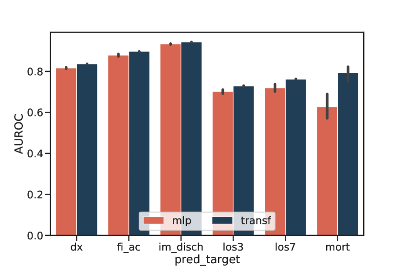
Figure 9: Prediction results according to the classifier backbone when $\textbf{z}\in\mathbb{R}^{2048}$ is compressed by a CNN-based one-stage encoder.

Table 1: Example of CNN-based encoder compressing $\textbf{E}_{input}\in\mathbb{R}^{8192\times 256}$ to $\textbf{E}_{output}\in\mathbb{R}^{64\times 8}$ following alg:CNNlayernum and 3.

Encoding	CNN-based
Input	$n=8192,d=256$ n’=64, d’=8
Build Layers	$r_{n}=log_{2}(8192/64)=7$ $r_{d}=log_{2}(256/8)=5$ $n_{l}=7$
Layer	Layer type	Output shape
1	$L_{nd}$	(4096,128)
2	$L_{nd}$	(2048,64)
3	$L_{nd}$	(1024,32)
4	$L_{nd}$	(512,16)
5	$L_{n}$	(256,16)
6	$L_{nd}$	(128,8)
7	$L_{n}$	(64,8)

Table 2: Example of Transformer-based encoder compressing $\textbf{E}_{input}\in\mathbb{R}^{8192\times 256}$ to $\textbf{E}_{output}\in\mathbb{R}^{64\times 8}$ according to alg:Transformer.

Encoding	Transformer-based
Input	$n=8192,d=256$ n’=64, d’=8, $n_{l}=4$
Build Layers	$r_{d}=log_{2}(256/8)=5$ $q=1,r=1$ $L_{d_{1}}$: decrease $d$ by $2^{2}$ $L_{d_{2}}$: decrease $d$ by $2^{1}$
Layer	Layer type	Output shape
1	$L_{d_{1}}$	(8192,64)
2	$L_{d_{2}}$	(8192,32)
3	$L_{d_{2}}$	(8192,16)
4	$L_{d_{2}}$	(8192,8)
-	$P_{adpt}$	(64,8)

Appendix E VQ-VAE

Stage 1. Learning a codebook

With the conventional VQ-VAE method, latent vector $\textbf{z}\in\mathbb{R}^{t\times c}$ consists of $t$ fibers, and each fiber $\textbf{z}^{i}\in\mathbb{R}^{c}$ is mapped to the nearest code. However, in order to improve the representation of each fiber, we divide each fiber into four pieces and replace each piece $\textbf{z}^{i,j}\in\mathbb{R}^{c/4}$ $(j\in 1,...,4)$ with its closest code from the codebook $\{\textbf{e}_{k}\}_{k=1}^{K}\in\mathbb{R}^{c/4}$ as follows:

$$\textbf{z}_{q}^{i,j}=\textbf{e}_{k}\ \text{where}\ k=\text{arg min}_{l}||\textbf{z}^{i,j}-\textbf{e}_{l}||$$

As a result, z is mapped into $\textbf{z}_{q}$ with $4t$ codes, and $\textbf{z}_{q}$ is fed to the decoder to reconstruct $\tilde{\textbf{x}}$.

The encoder, decoder, and codebook are trained in an end-to-end manner to minimize the distance between x, $\tilde{\textbf{x}}$ and z, $\textbf{z}_{q}$ respectively:

$$\mathcal{L}_{VQ}=||\textbf{x}-\tilde{\textbf{x}}||^{2}_{2}+||\text{sg}[\textbf{z}]-\textbf{z}_{q}||^{2}_{2}+\beta||\text{sg}[\textbf{z}_{q}]-\textbf{z}||^{2}_{2}$$

where sg$[\cdot]$ stands for the stop gradient operation, which supplements the non-differentiable quantization operation, and $\beta$ is a weight hyperparameter. In our case, we replace the second loss term with an exponential moving average for the codebook.

Stage 2. Learning a prior over discrete latents

We train the Transformer-based autoregressive model to learn the prior distribution over the discrete latent space:

$$p(\textbf{z}_{q})=\prod_{i}^{4t}p(\textbf{z}_{q,i}|\textbf{z}_{q,1},...,\textbf{z}_{q,i-1})$$

The autoregressive (AR) model predicts the next code based on past codes on every step to maximize the log-likelihood of the joint distribution of $p(\textbf{z}_{q})$:

$$\mathcal{L}_{AR}=\mathbb{E}_{\textbf{x}\sim p(\textbf{x})}[-\log{p(\textbf{z}_{q})}]$$

Finally, the sampled latent code sequence from $p(\textbf{z}_{q})$ is decoded to generate $\mathbf{\hat{x}}$.

Appendix F Qualitative Evaluation Method for Synthetic Data

Real data consists of samples representing patient data, and each sample consists of multiple events $\mathcal{E}_{R}$. Each event $e_{R}\in\mathcal{E}_{R}$, can be expressed as follows: $(\texttt{table},(\texttt{column name},\texttt{cell})\times\textit{n},\texttt{timegap})$, where n represents the number of columns for the event. Likewise, synthetic data consists of samples with multiple events $\mathcal{E}_{G}$. We evaluate the quality of synthetic data based on table syntax preservation and semantics consistency by comparing triples (table, column name, cell) in $\mathcal{E}_{G}$ to $\mathcal{E}_{R}$. The two-step procedure is as follows: (1) Definition of a set of triples (table, column name, content) based on $\mathcal{E}_{R}$, (2) Synthetic data evaluation based on pre-defined triples.

Definition of a set of triples

Each event $e_{R}$ is first split into triples of (table, column name, cell). Each cell can be categorized as either numeric or text-type. For the (table, column name) combinations of all resulting triples from $\mathcal{E}_{R}$, we remove duplicates and extract only the minimum and maximum values for numeric-type cells while performing tokenization for text-type cells. As a result, we build a refined set of triples (table, column name, content).

Synthetic data evaluation

for ${e}_{G}\in\mathcal{E}_{G}$ do

       // syntax check

       if not (order($e_{G}$) and column_pair($e_{G}$) and table_column($e_{G}$)) then

             return incorrect

            

       end if

      // semantics check

       for (column, content) in $e_{G}$ do

             if type(column) is numeric then

                   if not min_max(content) then

                         return incorrect

                        

                  

             else

                   if not sub_word(content) then

                         return incorrect

                        

                  

            

       end for

      return correct

      

end for

Algorithm 4 Qualitative Evaluation Metric for Synthetic Data

We define the functions of alg:Metric as follows:

To measure syntactic consistency, order checks whether $e_{G}$ starts with a table name. column_pair checks whether columns and contents consist in a pair. table_column checks whether the table and column names are in the pre-defined set.

To evaluate semantic consistency, for numeric-type cells, min_max checks whether the content lies within the minimum and maximum value of $(\texttt{table},\texttt{column name})$ in the pre-defined set. For the text-type cells, sub_word splits the cell values into subwords and then checks whether the split content is in the pre-defined set of $(\texttt{table},\texttt{column name})$.

Based on evaluation of each $e_{G}$ with alg:Metric, we use the 3 metrics below to report the synthetic data scores:

• RCE: ratio of correct events to total events

• RUE: ratio of correct unique events to total unique events

• RCS: ratio of correct samples to total samples

Specifically, RCE and RUE evaluate the number of correct events given all generated events on a non-unique and unique basis, respectively. RCS evaluates the number of correct patient samples out of all generated patient samples, in which each patient sample is a batch of events. By measuring the event-level and sample-level accuracy of synthetic data, we can analyze the consistency of synthetic data with real data.

Appendix G Additional results of qualitative evaluation (RUE)

We measured RUE metrics for synthetic data. Since RUE ignores duplicates and only considers unique events, it can measure the generative data from a different perspective than RCE. However, as shown in fig:RUE, it matches other metrics in section:Gen.

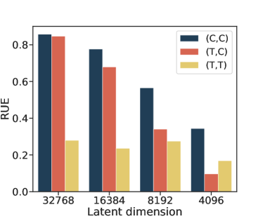
fig:qual_eval_RUE [RUE/mimic-III] [RUE/eicu]

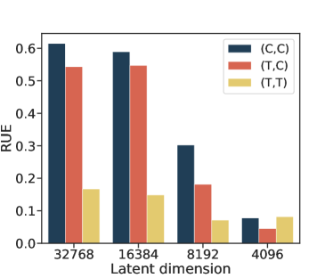
Figure 10: Quantitative evaluation on MIMIC-III and eICU datasets. RUE represents the ratio of correct unique events to total unique events.

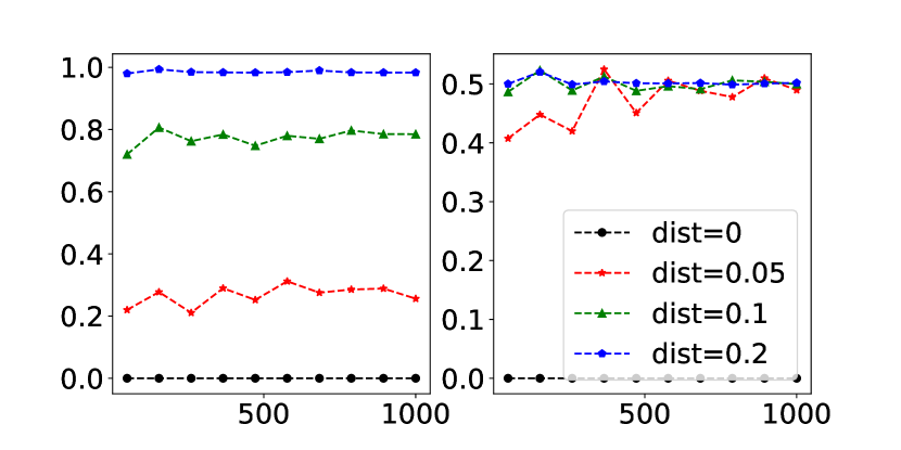
Figure 11: Recall (left) and precision (right) according to the number of real data that the attacker can access. The legend expressed Hamming distance threshold divided by the number of tokens.

Appendix H Privacy evaluation

Privacy evaluation is essential for assessing the quality of synthetic medical data. We conducted membership inference that measures the privacy leakage risk by determining whether the data generated by the model is similar enough to be considered a member of the training dataset.

We generated 1,000 records and sampled $n_{r}$ records each for train data and test data. The attacker has access to the real records of $2n_{r}$ and determines if each record was used for synthetic data creation via Hamming distance threshold between the two records. fig:MI shows recall and precision of membership inference for CNN-based VQ-VAE. Recall is the ratio from which members of a training set are correctly inferred as members by the attacker. Precision represents how many of the samples inferred as members are actually in training data set. Precision and recall are zero when Hamming distance threshold is zero, indicating that the synthetic data is not memorized by the model nor copied from the training data. A precision around 0.5, regardless of the $n_{r}$, suggests the attacker has poor membership inference performance.

Appendix I t-SNE visualization for different perplexity values

When using t-SNE for a qualitative evaluation, the interpretation may vary depending on the perplexity value, so we performed visualizations at various perplexities. The results displayed in fig:tsneppl demonstrate that increasing perplexity led to tighter clustering of the data points. Notably, the analysis conducted with multiple perplexity values yielded consistent results with those obtained in Section 5.3, which relied on a single perplexity value.

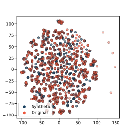
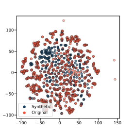
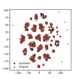
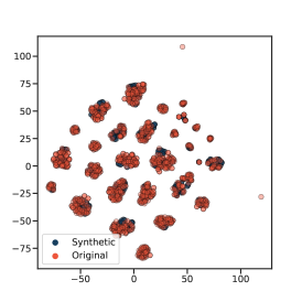
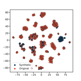
fig:tsneppl_mimic3 [(C,C) (PPL=1)][(T,C) (PPL=1)][(T,T) (PPL=1)]
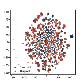
[(C,C) (PPL=5)][(T,C) (PPL=5)][(T,T) (PPL=5)]
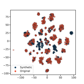
[(C,C) (PPL=10)][(T,C) (PPL=10)][(T,T) (PPL=10)]

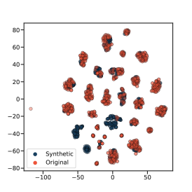
Figure 12: t-SNE visualization in latent space on MIMIC-III dataset according to perplexiy (PPL).

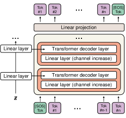
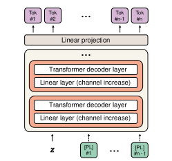
fig:TrnasfDecDesign [AR & CA] [non-AR & SA] [non-AR & SA+Unpool]

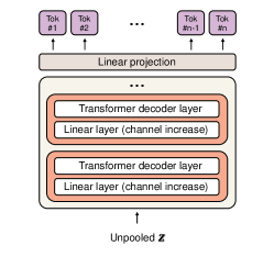
Figure 13: Transformer decoding scheme designs

Appendix J Transformer encoding schemes

As shown in alg:Transformer, our proposed Transformer encoding method gradually reduces the channel dimension as input x is passed through encoding layers. However, for Transformer-based encoding, it is common only to compress the temporal dimension (using [CLS] token or mean pooling) while leaving the channel dimension unchanged. Thus, we experiment and compare the temporal dimension compression to our channel compression method for reconstruction and prediction with z in 256 and 2048 dimensional spaces.

For $\textbf{z}\in\mathbb{R}^{1\times 256}$, the Transformer encoder layers process x and aggregate the temporal dimension into one by either extracting the [CLS] tokens or by mean pooling.

For $\textbf{z}\in\mathbb{R}^{1\times 2048}$, the output of the Transformer encoder is linearly projected into 2048 dimensions and then temporally compressed.

For $\textbf{z}\in\mathbb{R}^{8\times 256}$, we apply [CLS]-based and mean pooling-based compression with the following processes. For [CLS]-based compression, we insert 7 [CLS] tokens to the start of the sequence before encoding and subsequently use the 8 [CLS] tokens (i.e., encoded [CLS] output) for compression. We apply adaptive average pooling to the encoded outputs for mean pooling-based compression.

apd:TransfDecoding shows the results of reconstruction and prediction. For the reconstruction tasks, our encoding scheme outperforms all existing methods with a significant gap in accuracy for both l = 256 and l = 2048. Our method also shows comparable AUROC but slightly lower than mean pooling and higher AUROC than using [CLS].

Appendix K Transformer decoding schemes

We experiment on four different Transformer decoding schemes (shown in fig:TransfDec), including the setting in fig:transformerdecoder, where both the encoder and decoder are Transformers. After z is generated from the encoder, the decoder reconstructs input x by using either autoregressive or non-autoregressive methods. The autoregressive method generates x sequentially based on tokens from previous time steps, while the non-autoregressive method generates x at once.

For non-autoregressive decoding, z can be passed to the decoder either indirectly as a key for cross-attention (subsec:TaskSpecificModels) or directly for self-attention.

We use two different types of decoder inputs for self-attention. The first input type is a vector obtained by unpooling z to the length of input x, followed by adding positional encoding. Unpooling replicates adaptive mean pooling values for each pooling window by the size of the window. Also, positional encoding was added to overcome Transformer’s inability to distinguish tokens with identical values of different positions. The other input type is a vector of length x, created by concatenating placeholder tokens to z.

As shown in fig:TransfDecoding, autoregressive decoding shows the lowest reconstruction accuracy and does not appear to be suitable for reconstructing long sequences. Among the non-autoregressive decoding methods, the method of passing information of z from the encoder to the decoder through cross-attention shows the most efficient reconstruction.

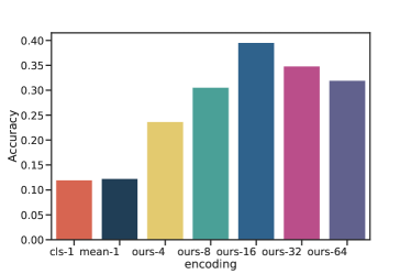
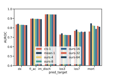
fig:comparisonTrnasformerEncdoing [Reconstruction ($l=256$)][Prediction ($l=256$)] [Reconstruction ($l=2048$)][Prediction ($l=2048$)]

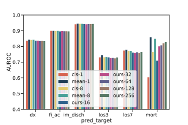
Figure 14: Comparison of Transformer encoding schemes.

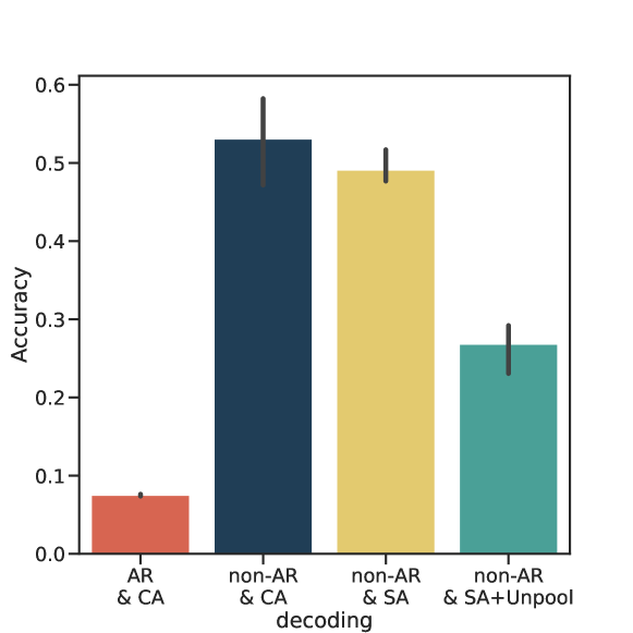
Figure 15: Reconstruction accuracy of various Transformer decoding schemes.

Appendix L Visualization and analysis of self-attention maps in Transformer

By visualizing the self-attention map of the Transformer layer having a hierarchical structure, we analyze how the reconstruction and prediction task differ from each other. Specifically, we choose a patient who has less than ten pad-events, which are fully filled with pad tokens, out of $n_{e}=256$ events. Then, we draw a heat-map for the first self-attention layer of the $\mathtt{Enc}^{e}$ in the autoencoder $(T,T)$ and the predictive model $\mathtt{Classifier}(\mathtt{Enc}_{struc}(\mathbf{x}))$. The patient’s key and query medical events respectively correspond to the y and x axes in the fig:sa.

As shown in the figure, Transformer shows an entirely different pattern in cases of reconstruction and prediction. For the reconstruction task illustrated in Figure 16, most of the attention heads in the Transformer mainly attend temporally proximal events represented by the elements near the diagonal line. However, almost every query event attends specific events out of all $n_{e}$ events to perform the clinical prediction task, as depicted both in fig:sapreddx and 16.

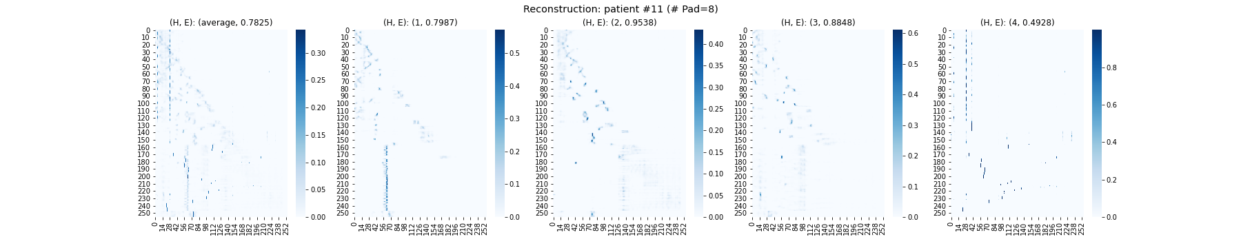
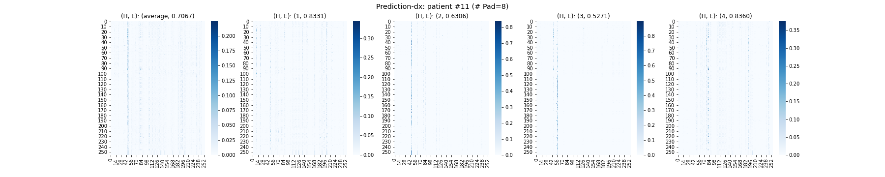
fig:selfattentionmap [Reconstruction] [Prediction-dx] [Prediction-mort]

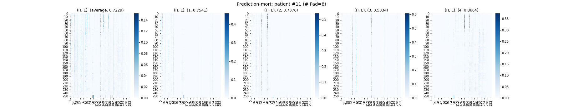
Figure 16: Self-attention heat-map of the $\mathtt{Enc}^{e}$ in the hierarchically-structured Transformer. In $\mathtt{Enc}^{e}$, the input for the patient has 256 medical events as query and key vectors. y and x axes in the figure respectively mean key and query event vector in each head. Query event vectors shows completely different pattern in reconstruction and prediction case.

Appendix M Results of each prediction task

fig:pred6Tasks-mimic-latent, 18, 19, and 20 show the prediction performances without averaging in a task-wise manner. Prediction performances are arranged by the latent dimension $l$ in fig:pred6Tasks-mimic-latent and 19, and by the temporal dimension $t$ in fig:pred6Tasks-mimic-temporal and 20. We report these performances of each subtask on both MIMIC-III and eICU datasets.

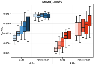
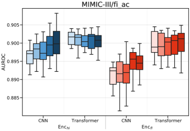
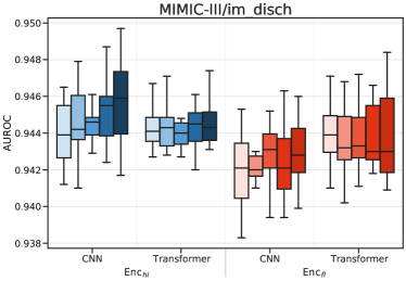
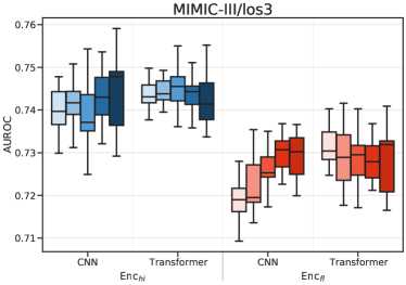
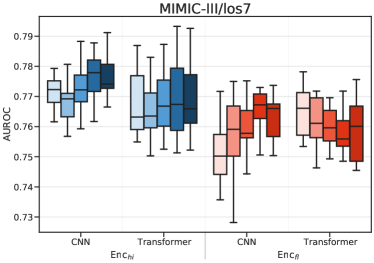
fig:prediction_arranged_by_latent [Diagnosis] [Final acuity] [Imminent Discharge] [Length-Of-Stay for case of three days] [Length-Of-Stay for case of seven days] [Mortality]

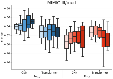
Figure 17: Prediction performances on MIMIC-III arranged by the latent dimension $l$

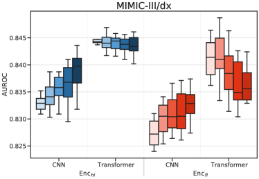
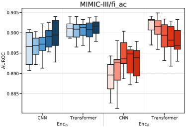
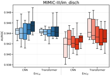
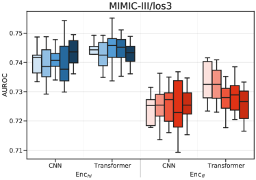
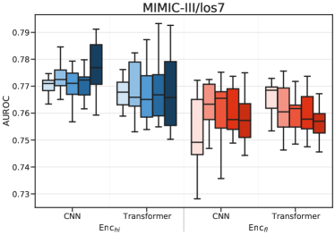
fig:prediction_aranged_by_temporal [Diagnosis][Final acuity] [Imminent Discharge][Length-Of-Stay for case of three days] [Length-Of-Stay for case of seven days][Mortality]

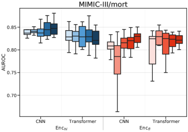
Figure 18: Prediction performances on MIMIC-III arranged by the temporal dimension $t$

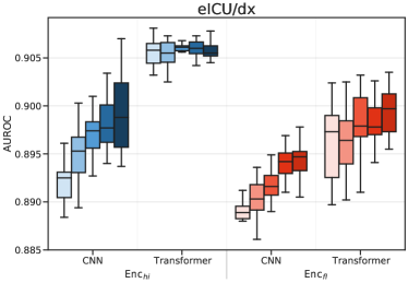
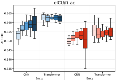
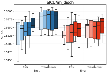
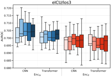
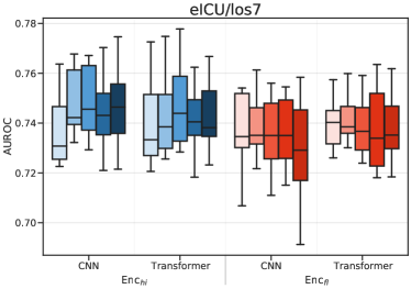
fig:prediction_eicu_latnet [Diagnosis][Final acuity] [Imminent Discharge][Length-Of-Stay for case of three days] [Length-Of-Stay for case of seven days][Mortality]

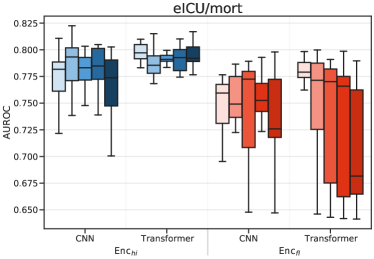
Figure 19: Prediction performances on eICU arranged by the latent dimension $l$

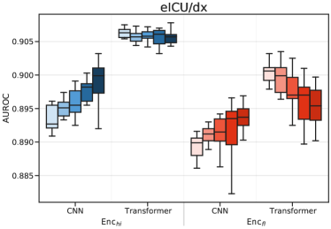
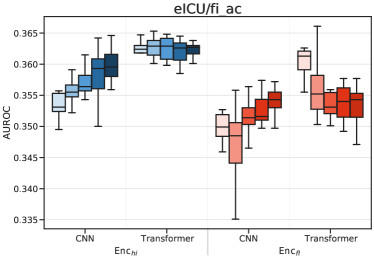
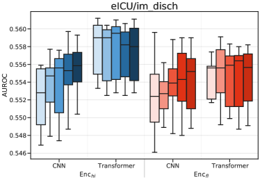
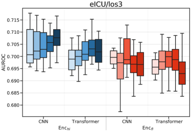
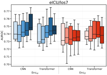
fig:prediction_eicu_temporal [Diagnosis][Final acuity] [Imminent Discharge][Length-Of-Stay for case of three days] [Length-Of-Stay for case of seven days][Mortality]

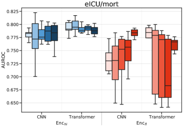
Figure 20: Prediction performances on eICU arranged by the temporal dimension $t$

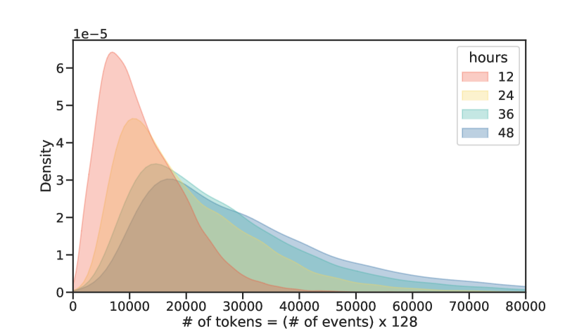
fig:kde_plot_mimic [Total number of tokens of hierarchical input] [Total number of tokens (excluding pad)]

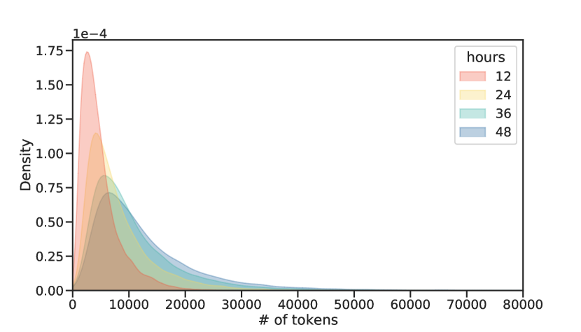
Figure 21: Kernel Density Estimate (KDE) plot visualizing the distribution of the total number of tokens according to observation time in the MIMIC-III dataset.

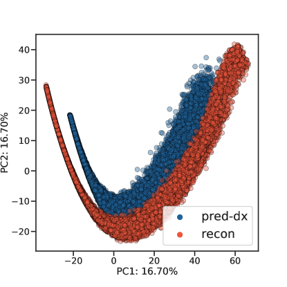
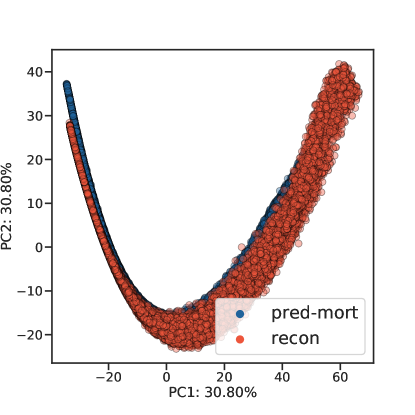
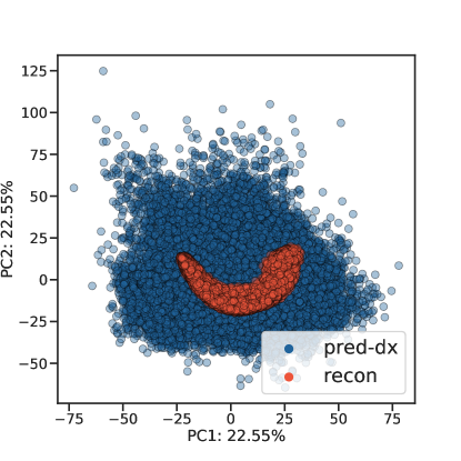
fig:pca_mimiciii [CNN-based (dx)][CNN-based (mort)] [Transformer-based (dx)][Transformer-based (mort)]

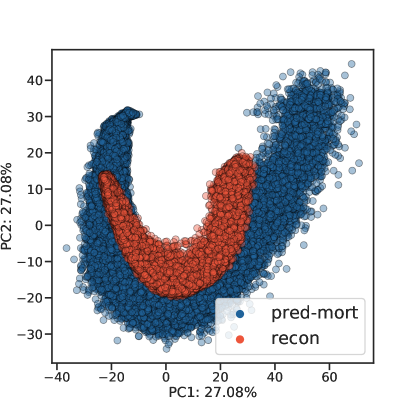
Figure 22: Visualization of latent vector using PCA on MIMIC-III dataset. Both CNN-based and Transformer-based encoders use CNN-based decoders for reconstruction.

References

- Choi et al. (2015) Edward Choi, Mohammad Taha Bahadori, Andy Schuetz, Walter F. Stewart, and Jimeng Sun. Doctor ai: Predicting clinical events via recurrent neural networks, 2015. URL https://arxiv.org/abs/1511.05942.
- Choi et al. (2019) Edward Choi, Zhen Xu, Yujia Li, Michael W. Dusenberry, Gerardo Flores, Yuan Xue, and Andrew M. Dai. Graph convolutional transformer: Learning the graphical structure of electronic health records. CoRR, abs/1906.04716, 2019. URL http://arxiv.org/abs/1906.04716.
- Choromanski et al. (2020) Krzysztof Choromanski, Valerii Likhosherstov, David Dohan, Xingyou Song, Andreea Gane, Tamas Sarlos, Peter Hawkins, Jared Davis, Afroz Mohiuddin, Lukasz Kaiser, et al. Rethinking attention with performers. arXiv preprint arXiv:2009.14794, 2020.
- Goldberger et al. (2000) Ary L Goldberger, Luis AN Amaral, Leon Glass, Jeffrey M Hausdorff, Plamen Ch Ivanov, Roger G Mark, Joseph E Mietus, George B Moody, Chung-Kang Peng, and H Eugene Stanley. Physiobank, physiotoolkit, and physionet: components of a new research resource for complex physiologic signals. circulation, 101(23):e215–e220, 2000.
- Hur et al. (2021) Kyunghoon Hur, Jiyoung Lee, Jungwoo Oh, Wesley Price, Young-Hak Kim, and Edward Choi. Unifying heterogenous electronic health records systems via text-based code embedding. CoRR, abs/2108.03625, 2021. URL https://arxiv.org/abs/2108.03625.
- Hur et al. (2022) Kyunghoon Hur, Jungwoo Oh, Junu Kim, Min Jae Lee, Eunbyeol Cho, Jiyoun Kim, Seong-Eun Moon, Young-Hak Kim, and Edward Choi. Unihpf : Universal healthcare predictive framework with zero domain knowledge, 2022. URL https://arxiv.org/abs/2207.09858.
- Johnson et al. (2019) A Johnson, T Pollard, O Badawi, et al. Eicu collaborative research database (version 2.0). PhysioNet, 2019.
- Johnson et al. (2016a) Alistair E. W. Johnson, Tom J. Pollard, and Roger G. Mark. MIMIC-III clinical database (version 1.4), 2016a.
- Johnson et al. (2016b) Alistair E. W. Johnson, Tom J. Pollard, Lu Shen, Li-wei H. Lehman, Mengling Feng, Mohammad Ghassemi, Benjamin Moody, Peter Szolovits, Leo Anthony Celi, and Roger G. Mark. MIMIC-III, a freely accessible critical care database. Scientific Data, 3(160035), 2016b. https://doi.org/10.1038/sdata.2016.35.
- Kingma and Ba (2014) Diederik P Kingma and Jimmy Ba. Adam: A method for stochastic optimization. arXiv preprint arXiv:1412.6980, 2014.
- Landi et al. (2020) Isotta Landi, Benjamin S Glicksberg, Hao-Chih Lee, Sarah Cherng, Giulia Landi, Matteo Danieletto, Joel T Dudley, Cesare Furlanello, and Riccardo Miotto. Deep representation learning of electronic health records to unlock patient stratification at scale. NPJ digital medicine, 3(1):1–11, 2020.
- Li et al. (2020) Yikuan Li, Shishir Rao, José Roberto Ayala Solares, Abdelaali Hassaine, Rema Ramakrishnan, Dexter Canoy, Yajie Zhu, Kazem Rahimi, and Gholamreza Salimi-Khorshidi. Behrt: transformer for electronic health records. Scientific reports, 10(1):1–12, 2020.
- Lipton et al. (2015) Zachary C Lipton, David C Kale, Charles Elkan, and Randall Wetzel. Learning to diagnose with lstm recurrent neural networks. arXiv preprint arXiv:1511.03677, 2015.
- Miotto et al. (2016) Riccardo Miotto, Li Li, Brian A Kidd, and Joel T Dudley. Deep patient: an unsupervised representation to predict the future of patients from the electronic health records. Scientific reports, 6(1):1–10, 2016.
- Nguyen et al. (2016) Phuoc Nguyen, Truyen Tran, Nilmini Wickramasinghe, and Svetha Venkatesh. Deepr: A convolutional net for medical records, 2016. URL https://arxiv.org/abs/1607.07519.
- Pollard et al. (2018) Tom J Pollard, Alistair EW Johnson, Jesse D Raffa, Leo A Celi, Roger G Mark, and Omar Badawi. The eicu collaborative research database, a freely available multi-center database for critical care research. Scientific data, 5(1):1–13, 2018.
- Rajkomar et al. (2018) Alvin Rajkomar, Eyal Oren, Kai Chen, Andrew M Dai, Nissan Hajaj, Michaela Hardt, Peter J Liu, Xiaobing Liu, Jake Marcus, Mimi Sun, et al. Scalable and accurate deep learning with electronic health records. NPJ digital medicine, 1(1):1–10, 2018.
- Rasmy et al. (2020) Laila Rasmy, Yang Xiang, Ziqian Xie, Cui Tao, and Degui Zhi. Med-bert: pre-trained contextualized embeddings on large-scale structured electronic health records for disease prediction, 2020. URL https://arxiv.org/abs/2005.12833.
- Shang et al. (2019) Junyuan Shang, Tengfei Ma, Cao Xiao, and Jimeng Sun. Pre-training of graph augmented transformers for medication recommendation. CoRR, abs/1906.00346, 2019. URL http://arxiv.org/abs/1906.00346.
- Shokri et al. (2017) Reza Shokri, Marco Stronati, Congzheng Song, and Vitaly Shmatikov. Membership inference attacks against machine learning models. In 2017 IEEE symposium on security and privacy (SP), pages 3–18. IEEE, 2017.
- Song et al. (2018) Huan Song, Deepta Rajan, Jayaraman Thiagarajan, and Andreas Spanias. Attend and diagnose: Clinical time series analysis using attention models. In Proceedings of the AAAI conference on artificial intelligence, volume 32, 2018.
- Van Den Oord et al. (2017) Aaron Van Den Oord, Oriol Vinyals, et al. Neural discrete representation learning. Advances in neural information processing systems, 30, 2017.
- Yoon et al. (2022) Jinsung Yoon, Michel Mizrahi, Nahid Ghalaty, Thomas Jarvinen, Ashwin Ravi, Peter Brune, Fanyu Kong, Dave Anderson, George Lee, Arie Meir, Farhana Bandukwala, Elli Kanal, Sercan Arik, and Tomas Pfister. Ehr-safe: Generating high-fidelity and privacy-preserving synthetic electronic health records. 2022. https://doi.org/10.21203/rs.3.rs-2347130/v1.