An alternative approach to optimal wire cutting
without ancilla qubits

Abstract

Wire cutting is a technique for partitioning large quantum circuits into smaller subcircuits in such a way that observables for the original circuits can be estimated from measurements on the smaller subcircuits. Such techniques provide workarounds for the limited numbers of qubits that are available on near-term quantum devices. Wire cutting, however, introduces multiplicative factors in the number of times such subcircuits need to be executed in order to estimate desired quantum observables to desired levels of statistical accuracy. An optimal wire-cutting methodology has recently been reported that uses ancilla qubits to minimize the multiplicative factors involved as a function of the number of wire cuts. Until just recently, the best-known wire-cutting technique that did not employ ancillas asymptotically converged to the same multiplicative factors, but performed significantly worse for small numbers of cuts. This latter technique also requires inserting measurement and state-preparation subcircuits that are randomly sampled from Clifford 2-designs on a per-shot basis. This paper presents a modified wire-cutting approach for pairs of subcircuits that achieves the same optimal multiplicative factors as wire cutting aided by ancilla qubits, but without requiring ancillas. The paper also shows that, while unitary 2-designs provide a sufficient basis for satisfying the decomposition, 2-designs are not mathematically necessary and alternative unitary designs can be constructed for the decompositions that are substantially smaller in size than 2-designs. As this paper was just about to be released, a similar result was published, so we also include a comparison of the two approaches.

1 Introduction

Current quantum computing devices implement limited numbers of qubits. If a quantum circuit requires more qubits than is available on a given device, the circuit cannot be executed directly. Various technical approaches have been developed to address this situation, one of which is known as wire cutting.

Wire cutting partitions a large quantum circuit into smaller subcircuits that can then execute on small quantum devices. Partitioning is achieved by “cutting” some of the connections between quantum gates, and then replacing those connections with measurement and state-preparation operations. By cutting a sufficient number of such connections, a set of disconnected subcircuits can be created, whereby each subcircuit can then be executed on a desired target device that implements a limited number of qubits. After execution, the measurements made for each subcircuit can be post-processed using classical computation to estimate a desired quantum observable for the overall circuit, almost as though the entire circuit was executed on a single, sufficiently large, quantum device without wire cutting.

However, wire cutting incurs a cost. Each cut introduces a multiplicative factor in the number of times the subcircuits need to be executed in order to estimate desired quantum observables to desired levels of statistical accuracy. Quantum observables are calculated classically by applying post-processing functions that map actual measurement outcomes (i.e., binary 1’s and 0’s) to real numbers and then averaging the resulting real numbers across multiple executions. The averaging serves to estimate expected values, and the statistical estimation errors in those estimates increase with each wire cut by multiplicative factors. To compensate, the number of circuit executions must then be increased by corresponding multiplicative factors in order to achieve the same levels of statistical accuracy as would be obtain without wire cutting. A central issue in wire-cutting research is to therefore develop measurement and state-preparation protocols that minimize the multiplicative factors incurred.

Wire cutting was originally proposed by Peng et al. [1]. The basic idea is to decompose the identity channel into a linear combination of measurement and state preparation operations. Wire cutting is performed by inserting an identity gate at the point where a cut is to be made, and then replacing the identity gate with its linear decomposition. The decomposition of the identity channel for a single qubit may be expressed mathematically as

$$\text{id}(\rho)=\rho=\sum_{j=1}^{T}c_{j}\rho^{j}\text{Tr}\left(O^{j}\rho\right)\;,$$ (1)

where each $O^{j}$ is a Hermitian observable, $\rho$ and $\rho^{j}$ are density matrices, and each $c_{j}$ is a real-valued coefficient. The observables $O^{j}$ correspond to measurements, while the density matrices $\rho^{j}$ correspond to state preparations. The coefficients $c_{j}$ are multiplying weights that are used when calculating the net overall observable for the original circuit from the measurements made on the partitioned subcircuits.

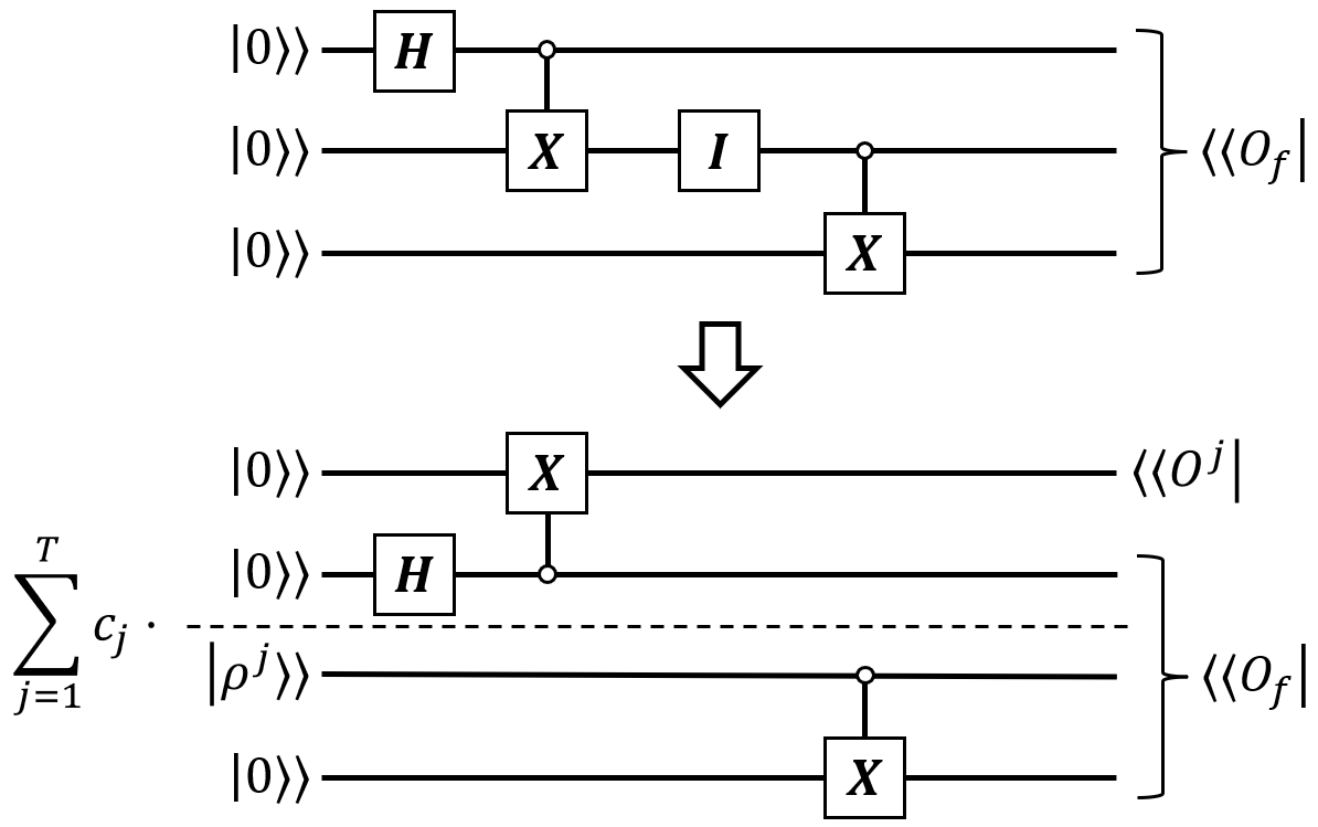
Figure 1: An example of performing wire cutting on a circuit where the objective is to estimate an observable $O_{f}$. An identity gate is inserted at the point where a wire cut is to be made. The gate is then replaced with its linear decomposition, which in this example results in two disconnected subcircuits and the introduction of an additional observable $O^{j}$ and state preparation $\rho^{j}$. The resulting subcircuits can be executed separately, with their measurements combined during post-processing to estimate the resulting overall observable $O^{j}\otimes O_{f}$ for the decomposed circuit.

Fig. 1 illustrates the wire cutting process for a simple circuit where the objective is to estimate an observable $O_{f}$. In this example, wire cutting creates two disconnected subcircuits and introduces an additional observable $O^{j}$ and state preparation $\rho^{j}$ per Eq. 1. If $\mathcal{U}$ is the channel implemented by the original circuit and if $\mathcal{U}_{A}$ and $\mathcal{U}_{B}$ are the channels implemented by the top and bottom disconnected subcircuits, respectively, then the expected value of $O_{f}$ can be expressed in terms of the expected values of the observables in the disconnected subcircuits as

$$\langle O_{f}\rangle=\text{Tr}\left(O_{f}\mathcal{U}(\rho_{0}^{\otimes 3})\right)=\sum_{j=1}^{T}c_{j}\text{Tr}\left((O^{j}\otimes O_{f})\left(\mathcal{U}_{A}(\rho_{0}^{\otimes 2})\otimes\mathcal{U}_{B}(\rho^{j}\otimes\rho_{0})\right)\right)\;,$$ (2)

where $\rho_{0}=\mathinner{\lvert{0}\rangle}\mathinner{\langle{0}\rvert}$.

A notable feature of the decomposition of Peng et al. is that the state preparations $\rho^{j}$ do not depend on the measurement outcomes of the observables $O^{j}$. The decomposition therefore does not require classical communication between subcircuits. The same is true of immediately subsequent work [2, 3, 4] in which variations on the same decomposition were proposed. A recent result by Brenner et al. [5] shows that, for any decomposition without communication, estimation errors must necessarily grow by multiplicative factors of at least $(4^{n})^{2}$ for $n$ wire cuts, where $(4^{n})^{2}$ is the optimum multiplicative factor achievable across all possible wire-cutting protocols without communication for $n$ wire cuts. The original decomposition of Peng et al. and its subsequent variations [2, 3, 4] all achieve this optimum.

To do better, classical communication must be employed. A more recent wire-cutting decomposition by Lowe et al. [6] does consider classical communication between subcircuits and achieves a multiplicative factor of $(2^{n+1}+1)^{2}$. Their approach combines two key insights.

• State preparations on one side of a wire cut can be made contingent on the measurement outcomes obtained on the other side of the cut, which requires communication and can lead to more efficient decompositions.

• When cutting several wires that connect two subcircuits, it is more efficient to decompose a single identity gate for the entire group of wires than it is to decompose separate identity gates, one for each individual wire being cut.

Thus, parallel cuts across $n$ qubits are treated as a single cut across a $d$-dimensional complex space, $d=2^{n}$. Their decomposition employs measure-and-prepare channels of the following form expressed in terms of unitaries $U\in\mathsf{U}(\mathbb{C}^{d})$ in dimension $d$

$$\Psi_{U}(\rho)=\sum_{k=1}^{d}\mathinner{\langle{k|U^{\dagger}\rho U|k}\rangle}U\mathinner{\lvert{k}\rangle}\mathinner{\langle{k}\rvert}U^{\dagger}\;.$$ (3)

Given a probability distribution $\{(p_{j},U_{j})\}$ over unitaries that forms a 2-design [7], they then define a pair of channels in dimension $d$

$$\Psi_{0}(\rho)=E_{U}[\Psi_{U}]=\sum_{j}p_{j}\sum_{k=1}^{d}\mathinner{\langle{k|U_{j}^{\dagger}\rho U_{j}|k}\rangle}U_{j}\mathinner{\lvert{k}\rangle}\mathinner{\langle{k}\rvert}U_{j}^{\dagger}$$ (4)

and

$$\Psi_{1}(\rho)={1\over d}\text{Tr}(\rho)\mathbbm{1}\;,$$ (5)

and they show that, if $Z$ is a Bernoulli random variable, $Z\in\{0,1\}$ with probability of outcome $1$ being $d/(2d+1)$, then

$$\text{id}(\rho)=(2d+1)E_{Z}\left[(-1)^{Z}\Psi_{Z}(\rho)\right]\;.$$ (6)

When cutting $n$ qubits, $d=2^{n}$ and the unitaries $U_{j}$ define paired measurement and state-preparation operations on the $n$ qubits being cut. The multiplicative factor affecting statistical estimation error is then $(2d+1)^{2}=(2^{n+1}+1)^{2}$.

Lowe et al. show that Eq. 6 holds for any probability distribution $\{(p_{j},U_{j})\}$ over unitaries that forms a 2-design. Such designs exist for all dimensions $d$ [7]. In particular, the uniform distribution over Clifford circuits forms a unitary 2-design, and it also forms a 3-design when the dimension $d$ is a power of two [8]. Lowe et al. recommend using uniformly random Clifford circuits as the 2-designs in their decomposition given that efficient methods exist for generating pseudorandom Clifford circuits [9]. Implementing this approach, however, would require generating and applying a separate Clifford circuit for each individual shot, which can be problematic for existing control circuitry.

This paper presents two improvements to the decomposition of Lowe et al. The first improvement is an alternative decomposition of the identity channel of the form

$$\text{id}(\rho)=(2d-1)E_{U}\left[\Phi_{U}(\rho)\right]\;.$$ (7)

The corresponding multiplicative factor is $(2d-1)^{2}=(2^{n+1}-1)^{2}$, which matches the optimal multiplicative factor achieved by Brenner et al. [5] using wire-cutting decompositions that leverage ancilla qubits, but in our case without using ancillas. It should be noted, however, that this improvement only pertains to wire cuts between individual pairs of subcircuits (i.e., “parallel” wire cuts), whereas the approach of Brenner et al. achieves this multiplicative factor across all wire cuts between a subcircuit and all of its neighbors in the resulting communication graph (i.e., “arbitrary” wire cuts). Nevertheless, the improvement presented here still offers a significant reduction in multiplicative factors versus Lowe et al., particularly for small numbers of wire cuts $n$.

The second improvement is that we show that the probability distribution $\{(p_{j},U_{j})\}$ over unitaries does not have to be a 2-design, and that it is in fact possible to construct alternative unitary designs $\{(p_{j},U_{j})\}$ that satisfy the decomposition that contain substantially fewer unitaries. In particular, we present an algorithm for constructing such unitary designs that, in experiments conducted thus far, has generated surprisingly compact designs.

This result is interesting from a theoretical perspective in that it establishes, by way of example, that unitary 2-designs are sufficient but not mathematically necessary in order to satisfy Eqs. 6 and 7. It is also interesting from a practical perspective in that the result raises the possibility of compiling compact libraries of unitary designs that can be used when applying Eqs. 6 and 7 in practice, thereby avoiding the need to generate uniformly random Clifford circuits on a per-run, per-shot basis.

As this paper was just about to be released, a very similar result was published by Harada et al. [10]. They employ a decomposition of the identity channel that can be written in quasiprobability form as

$$\text{id}(\rho)=(2d-1)\left(\sum_{j=1}^{d}{1\over 2d-1}\sum_{k=1}^{d}\mathinner{\langle{k|U_{j}^{\dagger}\rho U_{j}|k}\rangle}U_{j}\mathinner{\lvert{k}\rangle}\mathinner{\langle{k}\rvert}U_{j}^{\dagger}-{d-1\over 2d-1}\sum_{k=1}^{d}\mathinner{\langle{k|\rho|k}\rangle}\rho_{k}\right)\;,$$ (8)

where

$$\rho_{k}=\sum_{\ell=1}^{d}{1\over d-1}(1-\delta_{k,\ell})\mathinner{\lvert{\ell}\rangle}\mathinner{\langle{\ell}\rvert}\;,\qquad\delta_{i,j}=\begin{cases}1&i=j\\ 0&i\not=j\end{cases}\;,$$ (9)

and where $\{U_{j}\}_{j=1}^{d}\cup\{I^{\otimes n}\}$ denotes a set of unitary operators in dimension $d$ that transform the computational bases into $d+1$ mutually unbiased bases [11]. The corresponding multiplication factor is thus the same as that achieved here of $(2d-1)^{2}=(2^{n+1}-1)^{2}$ for $n$ qubits.

If we define $U_{0}=I^{\otimes n}$, Eq. 8 can be rewritten as

$$\text{id}(\rho) =(d+1)\sum_{j=0}^{d}{1\over d+1}\sum_{k=1}^{d}\mathinner{\langle{k|U_{j}^{\dagger}\rho U_{j}|k}\rangle}U_{j}\mathinner{\lvert{k}\rangle}\mathinner{\langle{k}\rvert}U_{j}^{\dagger}-d\left({1\over d}\text{Tr}(\rho)\mathbbm{1}\right)$$

$$=(2d+1)E_{Z}\left[(-1)^{Z}\Psi_{Z}(\rho)\right]\;.$$ (10)

Thus, the decomposition of Harada et al. can likewise be seen as an improvement to the decomposition of Lowe et al, where the corresponding unitary design is $\{(p,U_{j})\}_{j=0}^{d}$, and where $p=1/(d+1)$, $U_{0}=I^{\otimes n}$, and the unitary operators in the design transform the computational bases into $d+1$ mutually unbiased bases. Per Eq. 1, this unitary design likewise satisfies both the original decomposition of Lowe et al. and the decomposition presented here. Further relationships among these decompositions are discussed at the end of this paper.

2 Improvements to the Decomposition

An improved quasiprobability decomposition can be obtained by algebraically combining the depolarizing channel $\Psi_{1}$ in the decomposition of Lowe et al. with the measure-and-prepare channel $\Psi_{0}$ by replacing the pure-state preparations in $\Psi_{0}$ with mixed-state preparations, and by introducing a sign (i.e., $\pm 1$) term to account for the negative weighting assigned to the depolarizing channel $\Psi_{1}$ in Eq. 6. To define this mixed-state preparation, we define $q_{\ell|k}$ to be the conditional probability of preparing state $\mathinner{\lvert{\ell}\rangle}$ after measuring outcome $\mathinner{\lvert{k}\rangle}$, where

$$q_{\ell|k}=\begin{cases}{d\over 2d-1}&\ell=k\\ {1\over 2d-1}&\ell\not=k\end{cases}\;.$$ (11)

In addition, we define the sign multiplier $s_{\ell|k}$ to be

$$s_{\ell|k}=\begin{cases}1&\ell=k\\ -1&\ell\not=k\end{cases}\;.$$ (12)

We then define the signed mixed-state measure-and-prepare operation $\Phi_{U}$ to be

$$\Phi_{U}(\rho)=\sum_{k=1}^{d}\mathinner{\langle{k|U^{\dagger}\rho U|k}\rangle}\sum_{\ell=1}^{d}q_{\ell|k}s_{\ell|k}U\mathinner{\lvert{\ell}\rangle}\mathinner{\langle{\ell}\rvert}U^{\dagger}\;.$$ (13)

If it were not for the sign term $s_{\ell|k}$, $\Phi_{U}$ would be completely positive and trace preserving, but because of $s_{\ell|k}$ it is not. However, we can prove the following.

Lemma 2.1.

For any probability distribution $\{(p_{j},U_{j})\}$ over unitaries (not necessarily a 2-design), and for Bernoulli random variable $Z\in\{0,1\}$ with probability of outcome $1$ being $d/(2d+1)$, it is the case that

$$(2d-1)E_{U}\left[\Phi_{U}(\rho)\right]=(2d+1)E_{Z}\left[(-1)^{Z}\Psi_{Z}(\rho)\right]\;.$$ (14)

Proof.

From the above definitions we have

$$(2d-1)E_{U}\left[\Phi_{U}(\rho)\right] =\sum_{j}p_{j}\sum_{k=1}^{d}\mathinner{\langle{k|U_{j}^{\dagger}\rho U_{j}|k}\rangle}\sum_{\ell=1}^{d}(2d-1)q_{\ell|k}s_{\ell|k}U_{j}\mathinner{\lvert{\ell}\rangle}\mathinner{\langle{\ell}\rvert}U_{j}^{\dagger}$$

$$=\sum_{j}p_{j}\sum_{k=1}^{d}\mathinner{\langle{k|U_{j}^{\dagger}\rho U_{j}|k}\rangle}\left((d+1)U_{j}\mathinner{\lvert{k}\rangle}\mathinner{\langle{k}\rvert}U_{j}^{\dagger}-\sum_{\ell=1}^{d}U_{j}\mathinner{\lvert{\ell}\rangle}\mathinner{\langle{\ell}\rvert}U_{j}^{\dagger}\right)$$

$$=(d+1)\sum_{j}p_{j}\Psi_{U_{j}}(\rho)-d\sum_{j}p_{j}{1\over d}\text{Tr}(\rho)\mathbbm{1}$$

$$=(2d+1)\left({d+1\over 2d+1}\Psi_{0}-{d\over 2d+1}\Psi_{1}\right)$$

$$=(2d+1)E_{Z}\left[(-1)^{Z}\Psi_{Z}(\rho)\right]\;.$$ (15)

∎

Lemma 2.2.

For any 2-design $\{(p_{j},U_{j})\}$

$$\text{\rm id}(\rho)=(2d-1)E_{U}\left[\Phi_{U}(\rho)\right]$$ (16)

Proof.

Follows immediately from the above lemma and Lemma 2.1 in [6]. ∎

Algorithm 1 Single Monte Carlo Trial

Input: $f:\{0,1\}^{n}\rightarrow[-1,1]$, quantum circuit $C$ on $n$ qubits, unitary design $\{(p_{i},U_{i})\}$
      Output: Random Variable $Y$ s.t. $E[Y]=\text{Tr}(O_{f}\mathcal{N}(\rho_{0}^{\otimes n}))$

1:Initialize wires $A$ to $\mathinner{\lvert{0}\rangle}_{A}$

2:Apply circuit $C_{A}$ to wires $A$

3:$V\leftarrow$  unitary $U_{i}$ on $k$ qubits randomly drawn according to $\{(p_{i},U_{i})\}$

4:Apply circuit $V^{\dagger}$ to wires $A\cap B$

5:$y\leftarrow$  measurement of wires $A\cap B$

6:$x_{A}\leftarrow$  measurement of wires $[n]\setminus B$

7:$z\leftarrow\ell$ randomly drawn according to the conditional distribution $q_{\ell|y}$ defined in Eq. 18

8:Initialize wires $B$ to $\mathinner{\lvert{z}\rangle}_{A\cap B}\mathinner{\lvert{0}\rangle}_{[n]\setminus A}$

9:Apply circuit $V$ to wires $A\cap B$

10:Apply circuit $C_{B}$ to wires $B$

11:$x_{B}\leftarrow$  measurement of wires $B$

12:$x\leftarrow x_{A}x_{B}$

13:$Y\leftarrow(2^{k+1}-1)\,s_{z|y}\,f(x)$, where $s_{z|y}$ is defined in Eq. 12

14:return $Y$

In practice, the identity decomposition in Lemma 2.2 can be implemented as a Monte Carlo simulation that combines classical computation with quantum execution. An algorithm for implementing a single trial of this simulation is specified in pseudocode in Algorithm 1. This algorithm would then be executed multiple times and the resulting outputs $Y$ would be averaged over the resulting trials to estimate the expected value of a desired observable. Algorithm 1 borrows notation and terminology from Lowe et al. for ease of comparison. Thus, we consider an $n$-qubit circuit $C$ composed of subcircuits $C_{A},C_{B}$ acting on sets of qubits $A,B\subseteq[n]$, respectively, where $|A\cup B|=n$ and $|A\cap B|=k$. We also consider a diagonal observable $O_{f}$ with eigenvalues defined by a function $f:\{0,1\}^{n}\rightarrow[-1,1]$ such that $O_{f}=\sum_{x\in\{0,1\}^{n}}f(x)\mathinner{\lvert{x}\rangle}\mathinner{\langle{x}\rvert}$. The overall action of the quantum circuit $C$ is to implement a quantum channel denoted by $\mathcal{N}$, and the goal is therefore to estimate $\text{Tr}(O_{f}\mathcal{N}(\rho_{0}^{\otimes n}))$, $\rho_{0}=\mathinner{\lvert{0}\rangle}\mathinner{\langle{0}\rvert}$. The pseudocode notation in each line in Algorithm 1 likewise follows Lowe et al.

Comparing Algorithm 1 to Algorithm 1 of Lowe et al. [6], we can see that in both cases, a random variable $z$ is introduced that controls a stochastic initialization of wires $B$ prior to executing subcircuit $C_{B}$. The only significant procedural difference between the two algorithms is that this stochastic initialization is conditioned on the measurement outcome of subcircuit $C_{A}$ in the case of Algorithm 1 above, whereas it is independent of the measurement outcome in the case of Algorithm 1 in [6]. The mathematical consequences of this procedural difference are that, in the case of Algorithm 1 above, the output $Y$ is scaled by a factor $2^{k+1}-1$ and the sign change $s_{z|y}$ is conditioned on the measurement outcome of subcircuit $C_{A}$, whereas for Algorithm 1 in [6] the output $Y$ is scaled by a factor $2^{k+1}+1$ and the sign change $(-1)^{z}$ is independent of the measurement outcome of subcircuit $C_{A}$.

The scaling factors $2^{k+1}-1$ and $2^{k+1}+1$ correspond to the $\gamma$’s in the quasiprobability representations [12] of these decompositions of the identity channel. The importance of $\gamma$ for both algorithms is that the probability of the estimation error of the observable exceeding $\epsilon$ after averaging over $N$ trials can be bounded by the Hoeffding inequality using $\gamma$:

$$Pr\left\{\left|\text{Tr}(O_{f}\mathcal{N}(\rho_{0}^{\otimes n}))-{1\over N}\sum_{i=1}^{N}Y_{i}\right|\geq\epsilon\right\}\leq 2e^{-{N\epsilon^{2}\over 2\gamma^{2}}}\;.$$ (17)

Although the difference between $\gamma=2^{k+1}-1$ for Algorithm 1 above and $\gamma=2^{k+1}+1$ for Algorithm 1 in [6] becomes asymptotically negligible as the number of wire cuts $k$ gets large, for one wire cut it means a $\gamma$ of $3$ instead of $5$ and, hence, a multiplicative factor in the Hoeffding exponent of $9$ versus $25$. For two cuts it means a $\gamma$ of $7$ versus $9$ and a multiplicative factor of $49$ versus $81$. So, for small numbers of wire cuts, the statistical differences between the two are quite significant, with the decomposition presented here offering a substantial improvement over the decomposition presented in [6].

Algorithm 2 Alternative Single Monte Carlo Trial

Input: $f:\{0,1\}^{n}\rightarrow[-1,1]$, quantum circuit $C$ on $n$ qubits, unitary design $\{(p_{i},U_{i})\}$
      Output: Random Variable $Y$ s.t. $E[Y]=\text{Tr}(O_{f}\mathcal{N}(\rho_{0}^{\otimes n}))$

1:Initialize wires $A$ to $\mathinner{\lvert{0}\rangle}_{A}$

2:Apply circuit $C_{A}$ to wires $A$

3:$V\leftarrow$  unitary $U_{i}$ on $k$ qubits randomly drawn according to $\{(p_{i},U_{i})\}$

4:Apply circuit $V^{\dagger}$ to wires $A\cap B$

5:$y\leftarrow$  measurement of wires $A\cap B$

6:$x_{A}\leftarrow$  measurement of wires $[n]\setminus B$

7:$w\leftarrow 1$ with probabilty $2^{k}/(2^{k+1}-1)$, $0$ otherwise

8:if $w=0$ then

9:     Initialize wires $B$ to $\mathinner{\lvert{y}\rangle}_{A\cap B}\mathinner{\lvert{0}\rangle}_{[n]\setminus A}$

10:     $z\leftarrow y$

11:else

12:     Initialize wires $B$ to $\mathinner{\lvert{0}\rangle}_{A\cap B}\mathinner{\lvert{0}\rangle}_{[n]\setminus A}$

13:     Apply Hadamard gates to wires $A\cap B$

14:     $z\leftarrow$  measurement of wires $A\cap B$

15:end if

16:Apply circuit $V$ to wires $A\cap B$

17:Apply circuit $C_{B}$ to wires $B$

18:$x_{B}\leftarrow$  measurement of wires $B$

19:$x\leftarrow x_{A}x_{B}$

20:$Y\leftarrow(2^{k+1}-1)\,s_{z|y}\,f(x)$, where $s_{z|y}$ is defined in Eq. 12

21:return $Y$

It is worth noting that the random initialization defined in Steps 7 and 8 of Algorithm1 can also be implemented in a slightly different manner by leveraging the fact that the conditional probability distribution $q_{\ell|y}$ defined in Eq. 18 can be expressed as a mixture of a deterministic distribution and a uniformly random distribution

$$q_{\ell|k}=\left({d-1\over 2d-1}\right)q^{0}_{\ell|k}+\left({d\over 2d-1}\right)q^{1}_{\ell|k}\;,\qquad q^{0}_{\ell|k}=\begin{cases}1&\ell=k\\ 0&\ell\not=k\end{cases}\;,\qquad q^{1}_{\ell|k}={1\over d}\;.$$ (18)

Thus, initialing wires $A\cap B$ in circuit $C_{B}$ to $\mathinner{\lvert{\ell}\rangle}$ according to the distribution $q_{\ell|k}$ is equivalent to initializing those wires to $\mathinner{\lvert{k}\rangle}$ with probability $(d-1)/(2d-1)$ and to a uniformly random state (i.e., completely depolarized) with probability $d/(2d-1)$. The latter can be accomplished by initializing wires $A\cap B$ to the ground state $\mathinner{\lvert{0}\rangle}$, applying Hadamard gates, and then measuring those qubits.

Algorithm 2 embodies this alternative approach, which may be easier to implement on existing quantum devices than Algorithm 1. With this change, $\Phi_{U}$ in Eq. 2 is effectively being re-expressed as

$$\Phi_{U}(\rho) ={d-1\over 2d-1}\sum_{k=1}^{d}\mathinner{\langle{k|U^{\dagger}\rho U|k}\rangle}U\mathinner{\lvert{k}\rangle}\mathinner{\langle{k}\rvert}U^{\dagger}+{d\over 2d-1}\sum_{k=1}^{d}\mathinner{\langle{k|U^{\dagger}\rho U|k}\rangle}\sum_{\ell=1}^{d}s_{\ell|k}{1\over d}U\mathinner{\lvert{\ell}\rangle}\mathinner{\langle{\ell}\rvert}U^{\dagger}$$

$$=\left({d-1\over 2d-1}\right)\Psi_{U}+{d\over 2d-1}\sum_{k=1}^{d}\mathinner{\langle{k|U^{\dagger}\rho U|k}\rangle}\sum_{\ell=1}^{d}s_{\ell|k}{1\over d}U\mathinner{\lvert{\ell}\rangle}\mathinner{\langle{\ell}\rvert}U^{\dagger}\;,$$ (19)

where $\Psi_{U}$ is the measure-and-prepare channel of Lowe et al. defined in Eq. 3.

3 Improvements to the Unitary Design

Our second result demonstrates that, while unitary 2-designs are sufficient to satisfy the equational form of the decomposition proposed by Lowe et al., they are not mathematically necessary. The mapping from unitaries $U$ to measure-and-prepare channels $\Psi_{U}$ is, in fact, highly injective (i.e., many to one). There are two fundamental reasons:

• Measurements remove phase information, so unitaries that achieve the same amplitude magnitudes but with different phases during measurement will yield the same measurement outcomes.

• Two unitaries that are identical to within a permutation of the quantum state will also yield the same channel because the measure-and-prepare step at the heart of the operation effectively removes the effect of such permutations (e.g., a sequence of CNOT gates produces the same overall measure-and-prepare channel as the identity gate).

Consequently, any 2-design $\{(p_{i},U_{i})\}$ can be collapsed to produce a smaller design $\{(q_{j},V_{j})\}$, not necessarily a 2-design, that achieves the same decomposition, where

• The set of $V_{j}$’s is a subset of the $U_{i}$’s in the 2-design, with each $V_{j}$ defining an equivalence class of $U_{i}$’s that yield identical measure-and-prepare channels: $\Psi_{U_{i}}=\Psi_{V_{j}}$, $\Psi_{V_{j}}\not=\Psi_{V_{k}}$ for $j\not=k$.

• Each $q_{j}$ is the sum of the $p_{i}$’s for which $U_{i}$ produces the same channel as $V_{j}$, $q_{j}=\sum_{i:\Psi_{U_{i}}=\Psi_{V_{j}}}p_{i}$.

Just as one can perform an algorithmic search for efficient 2-designs (e.g., [13]), it is also possible to perform an algorithmic search for efficient unitary designs that satisfy the equational form of Lowe et al., at least for small numbers of cut wires such as one would encounter in practice. The basic approach would be to generate sets of circuits that yield distinct measure-and-prepare channels $\Psi_{U}$ and to simultaneously use linear techniques to find decompositions of the form

$$\text{id}=a_{0}\left(-\Psi_{1}\right)+\sum_{j=1}^{\mathcal{N}}a_{j}\Psi_{U_{j}}\;.$$ (20)

Such decompositions can then be directly related back to the decomposition of Lowe et al. as well as its refinement presented here.

Various linear techniques can be used to determine whether coefficients $a_{i}$ exist that satisfy the decomposition, and to also calculate their values:

• Ordinary least-squares linear regression can be used to find coefficients $a_{i}$ that can be either positive or negative.

• Non-negative least-squares linear regression can be used to find coefficients $a_{i}$ that are strictly non-negative.

• Linear programming can be used to find coefficients $a_{i}$ that minimize the sum of their absolute values $\gamma=\sum_{i}|a_{i}|$, where $\gamma$ then enters into the Hoeffding bound.

The squared errors returned by ordinary and non-negative least-squares can be used to determine when a sufficient number of measure-and-prepare channels $\Psi_{U}$ have been generated so that a solution then exists that satisfies the constraints of those methods. In that case, once the squared error falls below a desired tolerance (e.g., $10^{-12}$), the resulting coefficients can then be used as a solution to the decomposition. Linear programming, on the other hand, requires that the decomposition be introduced as a constraint when optimizing the coefficients. As such, linear programming can only be used once it has been determined, using one of the linear regression methods, that a sufficient number of measure-and-prepare channels have been generated.

To simplify the task of applying these linear techniques, we use a linear-algebra approach to represent the channels $\Psi_{1}$ and $\Psi_{U}$ as 4-dimensional tensors that can then be reshaped into the 1-dimensional column vectors needed by computer implementations of these linear techniques. The construction is provided by the following lemma.

Lemma 3.1.

Any linear transformation $T:\mathbb{C}^{m\times n}\rightarrow\mathbb{C}^{m\times n}$ over complex matrices $\mathbb{C}^{m\times n}$ can be equivalently represented as a 4-dimensional tensor $L^{T}$ such that, for all $A\in\mathbb{C}^{m\times n}$,

$$\left(T(A)\right)_{i,j}=\sum_{\ell,m}L^{T}_{i,j,\ell,m}A_{\ell,m}\;.$$ (21)

Proof.

We begin by noting that the set of $m\times n$ complex matrices is a vector space in and of itself without having to first “vectorize” the matrices. Specifically, for all matrices $A,B\in\mathbb{C}^{m\times n}$, scalars $a,b\in\mathbb{C}$, the zero matrix $0\in\mathbb{C}^{m\times n}$, and the unity scalar $1\in\mathbb{C}$:

$$A+B=B+A$$

(22)

In the usual manner, we define $\langle A,B\rangle=\sum_{i,j}\overline{A}_{i,j}B=\sum_{i,j}A^{*}_{i,j}B=Tr(A^{H}B)=Tr(A^{{\dagger}}B)$, where, depending on your preferred notation, $\overline{A}_{i,j}$ and $A^{*}_{i,j}$ are the complex conjugates of $A$, and $A^{H}$ and $A^{{\dagger}}$ are the conjugate (i.e., Hermitian) transposes of $A$. Then $\langle\cdot,\cdot\rangle$ is an inner product that is linear in the second argument. Specifically, for all matrices $A,B,C\in\mathbb{C}^{m\times n}$, scalars $a,b\in\mathbb{C}$, and the zero scalar $0\in\mathbb{R}$:

$$\langle A,B\rangle=\overline{\langle B,A\rangle}=\langle B,A\rangle^{*}$$

(23)

Consequently, if the set $\{\beta_{s}\}$ forms an orthonormal basis for $\mathbb{C}^{m\times n}$, then for any matrix $A\in\mathbb{C}^{m\times n}$,

$$A=\sum_{s}\beta_{s}\langle\beta_{s},A\rangle$$ (24)

Similarly, for any linear transformation $T:\mathbb{C}^{m\times n}\rightarrow\mathbb{C}^{m\times n}$

$$T(A)=\sum_{s}T(\beta_{s})\langle\beta_{s},A\rangle=\sum_{r}\sum_{s}\langle\beta_{r},T(\beta_{s})\rangle\beta_{r}\langle\beta_{s},A\rangle$$ (25)

When written using tensor indices, this equation becomes

$$\left(T(A)\right)_{i,j} =\sum_{r}\sum_{s}\langle\beta_{r},T(\beta_{s})\rangle\left(\beta_{r}\right)_{i,j}\langle\beta_{s},A\rangle$$

$$=\sum_{r}\sum_{s}\langle\beta_{r},T(\beta_{s})\rangle\left(\beta_{r}\right)_{i,j}\sum_{\ell,m}\left(\beta^{*}_{s}\right)_{\ell,m}A_{\ell,m}$$

$$=\sum_{\ell,m}\left(\sum_{r}\sum_{s}\langle\beta_{r},T(\beta_{s})\rangle\left(\beta_{r}\right)_{i,j}\left(\beta^{*}_{s}\right)_{\ell,m}\right)A_{\ell,m}$$

$$=\sum_{\ell,m}L^{T}_{i,j,\ell,m}\,A_{\ell,m}\;,$$ (26)

where

$$L^{T}_{i,j,\ell,m}=\sum_{r}\sum_{s}\langle\beta_{r},T(\beta_{s})\rangle\left(\beta_{r}\right)_{i,j}\left(\beta^{*}_{s}\right)_{\ell,m}\;.$$ (27)

Thus, all linear transformations $T$ over complex matrices can be equivalently represented as 4-dimensional tensors $L^{T}$, which have similar multiplication rules as matrices, except that the summations are taken over two indices instead of just one index. In terms of tensor operators, $L^{T}$ may be expressed as

$$L^{T}=\sum_{r}\sum_{s}\langle\beta_{r},T(\beta_{s})\rangle\beta_{r}\otimes_{\text{outer}}\beta^{*}_{s}\;,$$ (28)

where $\otimes_{\text{outer}}$ is the tensor outer product, not to be confused with the Kronecker product. It should be noted that the choice of orthonormal basis $\{\beta_{s}\}$ is irrelevant in the above construction: all choices yield the same tensor $L^{T}$. ∎

Because the above construction makes no assumptions regarding the nature of the linear transformations $T$, the construction can be directly applied in Liouville space, where the resulting tensors $L^{T}$ are the tensor representations of superoperators and the density matrices they operate on do not have to be “vectorized” (c.f., [14]).

The benefit of the tensor representation of superoperators is that it is then quite straight forward to construct the superoperator tensors for the channels in Eq. 20. In the case of the measure-and-prepare channel $\Psi_{U}$, if we write the equation $\rho^{\prime}=\Psi_{U}(\rho)=\sum_{k=1}^{d}\mathinner{\langle{k|U^{\dagger}\rho U|k}\rangle}U\mathinner{\lvert{k}\rangle}\mathinner{\langle{k}\rvert}U^{\dagger}$ in terms of tensor indices we obtain

$$\rho^{\prime}_{i,j} =\sum_{k=1}^{d}\sum_{\ell,m}U^{\dagger}_{k,\ell}\rho_{\ell,m}U_{m,k}U_{i,k}U^{\dagger}_{k,j}$$

$$=\sum_{\ell,m}\left(\sum_{k=1}^{d}U_{i,k}U^{*}_{j,k}U^{*}_{\ell,k}U_{m,k}\right)\rho_{\ell,m}$$

$$=\sum_{\ell,m}L^{\Psi_{U}}_{i,j,\ell,m}\,\rho_{\ell,m}\;,$$ (29)

where

$$L^{\Psi_{U}}_{i,j,\ell,m}=\sum_{k}U_{i,k}U^{*}_{j,k}U^{*}_{\ell,k}U_{m,k}\;.$$ (30)

Similarly, for the depolarizing channel $\rho^{\prime}=\Psi_{1}(\rho)={1\over d}\text{Tr}(\rho)\mathbbm{1}$ we obtain

$$\rho^{\prime}_{i,j} ={1\over d}\sum_{\ell,m}\delta_{\ell,m}\rho_{\ell,m}\delta_{i,j}$$

$$=\sum_{\ell,m}\left({1\over d}\delta_{i,j}\delta_{\ell,m}\right)\rho_{\ell,m}$$

$$=\sum_{\ell,m}L^{\Psi_{1}}_{i,j,\ell,m}\,\rho_{\ell,m}\;,$$ (31)

where

$$L^{\Psi_{1}}_{i,j,\ell,m}={1\over d}\,\delta_{i,j}\delta_{\ell,m}\;,\qquad\delta_{i,j}=\begin{cases}1&i=j\\ 0&i\not=j\end{cases}\;.$$ (32)

For the identity channel,

$$\rho^{\prime}_{i,j}=\sum_{\ell,m}\left(\delta_{i,\ell}\delta_{j,m}\right)\rho_{\ell,m}=\sum_{\ell,m}L^{\text{id}}_{i,j,\ell,m}\,\rho_{\ell,m}\;,\qquad L^{\text{id}}_{i,j,\ell,m}=\delta_{i,\ell}\delta_{j,m}\;.$$ (33)

Algorithm 3 Measure-and-Prepare Channel Generation for Unitary Designs

Input: number of qubits $n$, set of one-qubit gates $\mathcal{S}$, set of two-qubit gates $\mathcal{D}$, stopping criterion
      Output: set of unitaries $\mathcal{U}$, set of measure-and-prepare superoperator tensors $\mathcal{L}$

1:Initialize $\mathcal{U}\leftarrow\{I^{\otimes n}\},\mathcal{L}\leftarrow\{L^{\Psi_{I^{\otimes n}}}\}$

2:Initialize $Flag\leftarrow True$

3:while $Flag$ is $True$ and the stopping criterion has not been met do

4:     $Flag\leftarrow False$

5:     for $U\in\mathcal{U}$ do

6:         for $G\in\mathcal{S}$ and $k$ from 1 to $n$ do

7:              $V\leftarrow(I^{\otimes k-1}\otimes G\otimes I^{\otimes n-k})U$

8:              if $L^{\Psi_{V}}\notin\mathcal{L}$ then

9:                  $\mathcal{U}\leftarrow\mathcal{U}\cup\{G\}$

10:                  $\mathcal{L}\leftarrow\mathcal{L}\cup\{L^{\Psi_{V}}\}$

11:                  $Flag\leftarrow True$

12:              end if

13:         end for

14:         for $G\in\mathcal{D}$ do

15:              $V\leftarrow DU$

16:              if $L^{\Psi_{V}}\notin\mathcal{L}$ then

17:                  $\mathcal{U}\leftarrow\mathcal{U}\cup\{G\}$

18:                  $\mathcal{L}\leftarrow\mathcal{L}\cup\{L^{\Psi_{V}}\}$

19:                  $Flag\leftarrow True$

20:              end if

21:         end for

22:     end for

23:end while

24:return $\mathcal{U},\mathcal{L}$

The above definitions can be readily implemented using numerical packages that support tensor computations. The resulting 4-dimensional superoperator tensors can then be flattened into 1-dimensional vectors for use in solving Eq. 20. Specifically, flattened versions of $-L^{\Psi_{1}}$ and $L^{\Psi_{U_{j}}}$ for each value of $j$ would be assembled to form the columns of an “$A$” matrix, $L^{\text{id}}$ would become a “$b$” vector, and the coefficients in Eq. 20 would be obtained by solving linear equations of the form $Ax=b$.

Algorithm 3 defines a method for constructing sets of unitaries and their corresponding measure-and-prepare channels that can then be used to solve Eq. 20 as described above. A desired subgroup of unitaries from which to construct measure-and-prepare channels can be specified by providing the generating elements of the subgroup as input. In practice, when applying the resulting unitary designs in actual circuits, SWAP gates may be needed to move the wires that are to be cut to a connected subgraph of qubits on a target quantum device. Once moved, it would be preferable not to apply any additional SWAP gates when performing the measure-and-prepare operations needed for wire cutting. Algorithm 3 accommodates this need by requiring that two sets of generating elements be provided: a set of single-qubit gates $\mathcal{S}$ that can be applied to any qubit being cut, and a set of two-qubit gates $\mathcal{D}$ that are qubit-specific so that the connectivity graph of the target quantum device can be respected by supplying only those qubit combinations that are natively supported by the hardware. In this manner, Algorithm 3 can be used to generate customized unitary designs for specific regions of specific target devices.

A third input to Algorithm 3 is a stopping criterion. As described earlier, the squared errors returned by ordinary and non-negative least-squares can be used to determine when a sufficient number of measure-and-prepare channels $\Psi_{U}$ have been generated so that a solution then exists that satisfies the constraints of those methods. Once the squared error falls below a desired tolerance (e.g., $10^{-12}$), the resulting coefficients can then be used as a solution to the decomposition. This is then the stopping criterion used in the experiments conducted thus far, using either ordinary or non-negative least-squares regression, depending on the experiment.

Our initial experiments have focused on Clifford designs without device connectivity constraints. The single-qubit generating elements employed were thus Hadamard gates $H$ and phase gates $S$, while the two-qubit generators were CNOT gates across all pairs of qubits.

In our experience thus far in generating Clifford designs that satisfy Eq. 20, off-the-shelf ordinary least-squares regression (i.e., numpy.linalg.lstsq) identifies decompositions that require the fewest Clifford circuits, but the resulting $\gamma$’s (i.e., the sums of the absolute values of the regression coefficients) always seem to be greater than those obtained using non-negative least-squares and linear programming.

Off-the-shelf non-negative least-squares regression (i.e., scipy.optimize.nnls) seems to identify decompositions that require more Clifford circuits than ordinary least-squares, but the resulting $\gamma$’s are then identical to the $\gamma$’s discussed earlier for 2-designs, but using far fewer Clifford circuits. The resulting Clifford circuits and their coefficients are presented in Appendix A for 1, 2, 3, and 4 wire cuts. The numbers of unitaries in these designs are 3, 5, 28, and 136, respectively, as compared to the sizes of the corresponding Clifford groups, which are 8, 192, 92,160, and 743,178,240 [15]. Appendix A includes the associated probabilities of the resulting sets of Clifford circuits. All of these unitary designs satisfy both the original wire-cutting decomposition of Lowe et al. as well as the improved decomposition presented in the previous section.

Off-the-shelf linear programming (i.e., scipy.optimize.linprog) was only applied once a sufficient number of measure-and-prepare channels were generated for a solution to be obtained using non-negative least-squares regression. The linear programming solutions did not improve the resulting $\gamma$’s, but the solutions that were found were much larger in size than those obtained using non-negative least squares. Because these results are therefore inferior to those obtained using non-negative least-squares in terms of their sizes, they are not reported. Interestingly, all solutions found using linear programming also had non-negative coefficients, even though no constraints were added forcing the coefficients to be non-negative.

4 Comparisons with Harada et al.

One very interesting aspect of the decomposition just published by Harada et al. [10] is that the unitary designs they consider contain only $d+1=2^{n}+1$ unitaries, including the identity. Of the four designs presented in Appendix A, the first design for one qubit matches the design presented in [10]. The design for two qubits matches the size of the design reported in [10], but it does not include the identity circuit. The other two designs contain 28 and 136 unitaries for three and four-qubit wire cuts, respectively, versus the 9 and 17 unitaries that would be obtained by considering transformations from the computational bases to mutually unbiased bases. Because it is easy to constrain least-squares methods to include specific regressors, we re-executed our experiments to include the identity circuit and obtained the unitary designs presented in Appendix B. The resulting designs for three and four wire cuts then contained 17 and 122 unitaries, which is a mild improvement. However, the numbers of gates required to implement the unitaries then increased, which indicates that a trade-off must therefore exist between the number of unitaries that appear in a measure-and-prepare decomposition and the number of gates needed to implement those unitaries.

As mentioned in the Introduction, the unitary design presented by Harada et al. [10] also satisfies the decomposition presented here. From a practical point of view, the question then becomes which decomposition is easier to implement on a target quantum device. Algorithm 2 was introduced in Section 2 to provide an alternative means of preparing the mixed states that are needed so they can be more easily implemented on existing hardware. A similar type of mixed state appears in the decomposition of Harada et al. (see Eq. 9). A similar approach could potentially be used to handle this mixed state as was used in developing Algorithm 2. The resulting algorithm, though, would likely be very similar to Algorithm 2, since both decompositions are basically algebraic variations of each other.

5 Conclusions

With the modified decomposition presented here, the $\gamma$ factor that determines the rate of convergence of estimation errors for expected values of observables is reduced from $\gamma=2^{n+1}+1$ to $\gamma=2^{n+1}-1$, which matches the optimum $\gamma$ reported by Brenner et al. [5], but without using ancilla qubits in the wire cutting. This $\gamma$ also matches that of the recently published decomposition reported by Harada et al. [10].

The algorithms explored for constructing improved unitary designs produce much, much smaller sets of unitaries than 2-designs, which then makes both the original decomposition of Lowe al. [6], and the improved decomposition presented here, much more practical for real-world application. The algorithm for generating candidate measure-and-prepare channels allows custom sets of generating gates to be supplied as input, which then enables custom unitary designs to be generated that respect qubit connectivity patterns in specific regions of specific target devices. This capability could potentially be leveraged as an optimization when transpiling cut circuits to specific target devices. However, the sizes of the resulting unitary designs can be further improved as demonstrated by the unitary designs reported by Harada et al. [10]. Further research is therefore needed to produce custom unitary designs of comparable size that respect qubit connectivity patterns of target quantum devices.

Appendix A Appendix

The following are the unitary designs obtained for 1, 2, 3, and 4 wire cuts using non-negative least-squares regression. The sums of these coefficients match the value of $\gamma=2^{n+1}+1$ defined in the decomposition of Lowe et al. [6]. The probabilities define the corresponding unitary designs. All of these designs satisfy both the original decomposition of Lowe et al. and the improved decomposition presented in this paper.

A.1 One Wire Cut, 3 Unitaries

Coefficient	Probabilty	PseudoQASM Circuit	Num Gates
2.000000		Complete Depolarization
1.000000	0.33333333	Identity Circuit	0
1.000000	0.33333333	h 0;	1
1.000000	0.33333333	h 0; s 0;	2

A.2 Two Wire Cuts, 5 Unitaries

Coefficient	Probabilty	PseudoQASM Circuit	Num Gates
4.000000		Complete Depolarization
1.000000	0.20000000	h 0; h 1;	2
1.000000	0.20000000	h 0; s 0;	2
1.000000	0.20000000	h 1; s 1;	2
1.000000	0.20000000	h 0; s 0; cx 0, 1;	3
1.000000	0.20000000	h 0; cx 0, 1; h 0;	3

A.3 Three Wire Cuts, 28 Unitaries

Coefficient	Probabilty	PseudoQASM Circuit	Num Gates
8.000000		Complete Depolarization
0.500000	0.05555556	h 0; h 1; h 2;	3
0.125000	0.01388889	h 0; h 1; cx 1, 2;	3
0.500000	0.05555556	h 0; s 0; cx 0, 2;	3
0.625000	0.06944444	h 0; cx 0, 1; h 0;	3
0.125000	0.01388889	h 0; h 1; s 0; s 1;	4
0.375000	0.04166667	h 0; h 1; s 0; cx 0, 2;	4
0.250000	0.02777778	h 0; h 1; s 0; cx 1, 0;	4
0.125000	0.01388889	h 0; h 2; s 0; s 2;	4
0.250000	0.02777778	h 0; h 2; s 0; cx 2, 0;	4
0.125000	0.01388889	h 0; s 0; cx 0, 2; h 2;	4
0.250000	0.02777778	h 1; h 2; s 1; s 2;	4
0.125000	0.01388889	h 1; h 2; s 1; cx 2, 1;	4
0.625000	0.06944444	h 1; s 1; cx 1, 2; h 2;	4
0.375000	0.04166667	h 0; h 1; s 0; s 1; cx 1, 2;	5
0.125000	0.01388889	h 0; h 1; s 0; cx 0, 2; h 0;	5
0.375000	0.04166667	h 0; h 1; s 0; cx 1, 2; h 1;	5
0.625000	0.06944444	h 0; h 1; s 1; cx 0, 2; h 0;	5
0.250000	0.02777778	h 0; h 1; s 1; cx 0, 2; cx 1, 0;	5
0.375000	0.04166667	h 0; h 1; s 1; cx 1, 2; h 1;	5
0.250000	0.02777778	h 0; h 1; cx 0, 2; h 0; cx 1, 0;	5
0.250000	0.02777778	h 0; h 1; cx 0, 2; h 0; cx 1, 2;	5
0.625000	0.06944444	h 0; h 2; s 0; s 2; cx 0, 1;	5
0.375000	0.04166667	h 0; h 2; s 0; cx 0, 1; h 0;	5
0.125000	0.01388889	h 0; h 2; s 0; cx 0, 1; h 1;	5
0.375000	0.04166667	h 0; h 2; s 0; cx 2, 0; cx 0, 1;	5
0.125000	0.01388889	h 0; s 0; cx 0, 1; h 0; cx 0, 2;	5
0.500000	0.05555556	h 0; s 0; cx 0, 1; h 1; cx 1, 2;	5
0.250000	0.02777778	h 0; cx 0, 1; h 0; cx 0, 2; cx 1, 0;	5

A.4 Four Wire Cuts, 136 Unitaries

Coefficient	Probabilty	PseudoQASM Circuit	Num Gates
16.000000		Complete Depolarization
0.077381	0.00455182	h 0; h 1; s 0; cx 0, 3; h 3;	5
0.177954	0.01046790	h 0; h 1; s 1; cx 0, 2; cx 1, 0;	5
0.117719	0.00692462	h 0; h 2; s 0; cx 0, 3; h 0;	5
0.070027	0.00411922	h 0; h 2; s 0; cx 0, 3; cx 2, 0;	5
0.018012	0.00105952	h 0; h 2; s 0; cx 0, 3; cx 2, 3;	5
0.089097	0.00524098	h 0; h 2; s 2; cx 0, 1; cx 2, 3;	5
0.071553	0.00420902	h 0; h 3; s 0; cx 0, 1; h 1;	5
0.105949	0.00623232	h 1; h 2; s 2; cx 2, 3; h 3;	5
0.072323	0.00425430	h 0; h 1; h 2; h 3; s 0; cx 1, 0;	6
0.084937	0.00499627	h 0; h 1; h 2; h 3; s 1; cx 2, 1;	6
0.054453	0.00320312	h 0; h 1; h 2; h 3; s 2; cx 3, 2;	6
0.048801	0.00287065	h 0; h 1; h 2; s 0; cx 2, 0; cx 2, 3;	6
0.182626	0.01074273	h 0; h 1; h 3; s 0; s 1; cx 3, 0;	6
0.057030	0.00335469	h 0; h 1; h 3; s 0; s 3; cx 0, 2;	6
0.081442	0.00479070	h 0; h 1; h 3; s 0; s 3; cx 1, 0;	6
0.178872	0.01052189	h 0; h 1; h 3; s 1; s 3; cx 1, 2;	6
0.023948	0.00140871	h 0; h 1; s 0; s 1; cx 1, 2; h 1;	6
0.099682	0.00586366	h 0; h 1; s 0; cx 0, 2; h 0; cx 1, 2;	6
0.055007	0.00323569	h 0; h 1; s 0; cx 0, 2; h 2; cx 1, 0;	6
0.065589	0.00385817	h 0; h 1; s 0; cx 0, 2; cx 1, 0; h 0;	6
0.026757	0.00157396	h 0; h 1; s 0; cx 0, 2; cx 1, 0; cx 1, 3;	6
0.137451	0.00808535	h 0; h 1; s 0; cx 0, 2; cx 1, 2; h 2;	6
0.307929	0.01811345	h 0; h 1; s 0; cx 0, 3; h 0; cx 0, 2;	6
0.108920	0.00640705	h 0; h 1; s 0; cx 0, 3; h 0; cx 1, 3;	6
0.034429	0.00202525	h 0; h 1; s 0; cx 0, 3; h 3; cx 1, 0;	6
0.156286	0.00919332	h 0; h 1; s 0; cx 0, 3; cx 1, 0; cx 1, 2;	6
0.069658	0.00409751	h 0; h 1; s 1; cx 0, 2; cx 0, 3; cx 1, 0;	6
0.300465	0.01767439	h 0; h 1; s 1; cx 0, 2; cx 0, 3; cx 1, 2;	6
0.342935	0.02017266	h 0; h 1; s 1; cx 0, 3; cx 1, 0; h 1;	6
0.351542	0.02067894	h 0; h 1; s 1; cx 1, 2; h 1; cx 1, 3;	6
0.231054	0.01359143	h 0; h 1; s 1; cx 1, 3; h 1; cx 1, 2;	6
0.056278	0.00331044	h 0; h 1; cx 0, 2; h 0; cx 0, 3; cx 1, 3;	6
0.054619	0.00321287	h 0; h 1; cx 0, 2; h 0; cx 1, 0; cx 1, 3;	6
0.055383	0.00325779	h 0; h 1; cx 0, 2; h 0; cx 1, 3; cx 2, 1;	6
0.128292	0.00754657	h 0; h 1; cx 0, 2; cx 0, 3; h 3; cx 1, 2;	6
0.068560	0.00403294	h 0; h 1; cx 0, 2; cx 0, 3; cx 1, 2; h 1;	6
0.132793	0.00781133	h 0; h 1; cx 0, 3; h 0; cx 1, 0; cx 1, 2;	6
0.171234	0.01007257	h 0; h 1; cx 0, 3; cx 1, 0; cx 1, 2; h 1;	6
0.111486	0.00655800	h 0; h 2; h 3; s 0; s 3; cx 0, 1;	6
0.049308	0.00290046	h 0; h 2; h 3; s 0; s 3; cx 2, 0;	6
0.067551	0.00397362	h 0; h 2; h 3; s 0; cx 2, 0; cx 0, 1;	6
0.067291	0.00395829	h 0; h 2; s 0; s 2; cx 0, 3; h 0;	6
0.278136	0.01636096	h 0; h 2; s 0; cx 0, 1; h 0; cx 0, 3;	6
0.172267	0.01013333	h 0; h 2; s 0; cx 0, 1; h 1; cx 1, 3;	6
0.040293	0.00237016	h 0; h 2; s 0; cx 0, 3; cx 2, 0; cx 0, 1;	6
0.107591	0.00632888	h 0; h 2; s 0; cx 0, 3; cx 2, 3; h 2;	6
0.232530	0.01367821	h 0; h 2; s 2; cx 0, 3; h 0; cx 2, 3;	6
0.088464	0.00520376	h 0; h 2; cx 0, 1; cx 0, 3; cx 2, 3; h 3;	6
0.146617	0.00862451	h 0; h 2; cx 0, 3; h 0; cx 2, 0; cx 0, 3;	6
0.095580	0.00562235	h 0; h 3; s 0; cx 0, 2; h 0; cx 0, 1;	6
0.012711	0.00074768	h 1; h 2; h 3; s 1; s 2; cx 3, 2;	6
0.036036	0.00211979	h 1; h 2; h 3; s 1; s 3; cx 2, 1;	6
0.180186	0.01059920	h 1; h 2; s 1; cx 1, 3; h 1; cx 2, 3;	6
0.226670	0.01333355	h 1; h 2; s 1; cx 1, 3; h 3; cx 2, 1;	6
0.176104	0.01035906	h 1; h 2; s 2; cx 1, 3; cx 2, 1; h 2;	6
0.193634	0.01139026	h 0; h 1; h 2; s 0; s 1; cx 0, 3; cx 2, 0;	7
0.311273	0.01831017	h 0; h 1; h 2; s 0; s 1; cx 2, 3; h 2;	7
0.138706	0.00815915	h 0; h 1; h 2; s 0; s 2; cx 0, 3; cx 1, 3;	7
0.125152	0.00736191	h 0; h 1; h 2; s 0; s 2; cx 1, 0; cx 1, 3;	7
0.104305	0.00613559	h 0; h 1; h 2; s 0; s 2; cx 1, 0; cx 2, 3;	7
0.112402	0.00661191	h 0; h 1; h 2; s 0; s 2; cx 1, 3; cx 2, 1;	7
0.149947	0.00882044	h 0; h 1; h 2; s 0; cx 0, 3; cx 1, 3; cx 2, 1;	7
0.104210	0.00612999	h 0; h 1; h 2; s 0; cx 1, 0; cx 0, 3; cx 2, 3;	7
0.111984	0.00658729	h 0; h 1; h 2; s 0; cx 2, 0; cx 0, 3; h 0;	7
0.104404	0.00614139	h 0; h 1; h 2; s 0; cx 2, 0; cx 2, 3; h 2;	7
0.203606	0.01197682	h 0; h 1; h 2; s 1; s 2; cx 0, 3; h 0;	7
0.099142	0.00583188	h 0; h 1; h 2; s 1; s 2; cx 1, 3; h 3;	7
0.132070	0.00776880	h 0; h 1; h 2; s 2; cx 0, 3; h 0; cx 2, 0;	7
0.069135	0.00406678	h 0; h 1; h 2; s 2; cx 0, 3; cx 1, 0; cx 2, 0;	7
0.083391	0.00490533	h 0; h 1; h 3; s 0; s 1; cx 1, 2; h 1;	7
0.208424	0.01226026	h 0; h 1; h 3; s 0; s 1; cx 1, 2; h 2;	7
0.018317	0.00107749	h 0; h 1; h 3; s 0; s 1; cx 1, 2; cx 3, 0;	7
0.100713	0.00592429	h 0; h 1; h 3; s 0; s 1; cx 3, 0; cx 0, 1;	7
0.096150	0.00565587	h 0; h 1; h 3; s 0; s 1; cx 3, 0; cx 0, 2;	7
0.003405	0.00020032	h 0; h 1; h 3; s 0; s 3; cx 1, 0; cx 0, 2;	7
0.260562	0.01532716	h 0; h 1; h 3; s 0; s 3; cx 1, 2; h 1;	7
0.121145	0.00712619	h 0; h 1; h 3; s 0; cx 1, 0; cx 1, 2; h 2;	7
0.039427	0.00231925	h 0; h 1; h 3; s 0; cx 3, 0; cx 0, 2; cx 1, 0;	7
0.036867	0.00216862	h 0; h 1; h 3; s 1; cx 0, 2; cx 1, 0; h 1;	7
0.197091	0.01159358	h 0; h 1; s 0; s 1; cx 0, 2; h 0; cx 0, 1;	7
0.243278	0.01431048	h 0; h 1; s 0; s 1; cx 0, 2; h 2; cx 2, 1;	7
0.057754	0.00339732	h 0; h 1; s 0; cx 0, 2; h 0; cx 0, 3; cx 1, 0;	7
0.096286	0.00566388	h 0; h 1; s 0; cx 0, 2; h 0; cx 1, 0; cx 0, 3;	7
0.051346	0.00302035	h 0; h 1; s 0; cx 0, 2; h 0; cx 1, 2; cx 1, 3;	7
0.023306	0.00137093	h 0; h 1; s 0; cx 0, 2; h 0; cx 1, 2; cx 2, 3;	7
0.219133	0.01289015	h 0; h 1; s 0; cx 0, 2; h 0; cx 1, 3; h 1;	7
0.118390	0.00696409	h 0; h 1; s 0; cx 0, 2; h 0; cx 2, 3; cx 1, 2;	7
0.342627	0.02015455	h 0; h 1; s 0; cx 0, 2; h 2; cx 0, 3; cx 1, 0;	7
0.047876	0.00281621	h 0; h 1; s 0; cx 0, 2; h 2; cx 0, 3; cx 1, 3;	7
0.380592	0.02238779	h 0; h 1; s 0; cx 0, 2; h 2; cx 1, 2; cx 2, 3;	7
0.224981	0.01323416	h 0; h 1; s 0; cx 0, 2; h 2; cx 1, 3; h 1;	7
0.055010	0.00323590	h 0; h 1; s 0; cx 0, 2; cx 0, 3; cx 1, 2; h 1;	7
0.061342	0.00360834	h 0; h 1; s 0; cx 0, 2; cx 1, 0; cx 1, 3; h 1;	7
0.009913	0.00058309	h 0; h 1; s 0; cx 0, 2; cx 1, 0; cx 1, 3; h 3;	7
0.006922	0.00040716	h 0; h 1; s 0; cx 0, 2; cx 1, 2; cx 1, 3; h 1;	7
0.113841	0.00669654	h 0; h 1; s 0; cx 0, 2; cx 1, 2; cx 1, 3; h 3;	7
0.249738	0.01469046	h 0; h 1; s 0; cx 0, 3; h 3; cx 1, 0; cx 0, 2;	7
0.242043	0.01423783	h 0; h 1; s 0; cx 0, 3; h 3; cx 1, 2; cx 1, 3;	7
0.020993	0.00123491	h 0; h 1; s 0; cx 1, 0; cx 1, 2; h 1; cx 1, 3;	7
0.149748	0.00880871	h 0; h 1; s 0; cx 1, 0; cx 1, 2; h 1; cx 2, 3;	7
0.001248	0.00007342	h 0; h 1; s 1; cx 0, 2; h 0; cx 1, 0; cx 0, 3;	7
0.337875	0.01987501	h 0; h 1; s 1; cx 0, 2; h 0; cx 1, 3; h 1;	7
0.332991	0.01958770	h 0; h 1; s 1; cx 0, 2; h 0; cx 1, 3; h 3;	7
0.139003	0.00817666	h 0; h 1; s 1; cx 0, 2; cx 0, 3; cx 1, 3; h 1;	7
0.002701	0.00015886	h 0; h 1; s 1; cx 0, 2; cx 1, 0; h 1; cx 1, 3;	7
0.133693	0.00786431	h 0; h 1; s 1; cx 0, 2; cx 1, 3; h 1; cx 1, 0;	7
0.151284	0.00889903	h 0; h 1; s 1; cx 0, 2; cx 1, 3; h 3; cx 3, 0;	7
0.116149	0.00683229	h 0; h 1; s 1; cx 0, 3; h 0; cx 1, 2; h 2;	7
0.052431	0.00308417	h 0; h 1; s 1; cx 0, 3; cx 1, 0; cx 1, 2; h 2;	7
0.078384	0.00461084	h 0; h 1; s 1; cx 0, 3; cx 1, 2; h 1; cx 1, 0;	7
0.085250	0.00501469	h 0; h 1; cx 0, 2; h 0; cx 0, 3; cx 1, 3; cx 2, 0;	7
0.156046	0.00917916	h 0; h 1; cx 0, 2; h 0; cx 0, 3; cx 2, 0; cx 1, 2;	7
0.200294	0.01178202	h 0; h 1; cx 0, 2; h 0; cx 1, 0; cx 0, 2; cx 0, 3;	7
0.097268	0.00572162	h 0; h 1; cx 0, 2; h 0; cx 1, 0; cx 0, 2; cx 1, 3;	7
0.134494	0.00791138	h 0; h 1; cx 0, 2; h 0; cx 1, 0; cx 0, 2; cx 2, 3;	7
0.146746	0.00863209	h 0; h 1; cx 0, 2; cx 0, 3; cx 1, 3; h 1; cx 0, 1;	7
0.184532	0.01085485	h 0; h 1; cx 0, 2; cx 1, 0; cx 1, 3; h 1; cx 1, 0;	7
0.040634	0.00239023	h 0; h 1; cx 0, 3; h 0; cx 1, 0; cx 0, 3; cx 1, 2;	7
0.045664	0.00268612	h 0; h 2; h 3; s 0; s 2; cx 0, 1; h 0;	7
0.001225	0.00007205	h 0; h 2; h 3; s 0; s 2; cx 0, 1; h 1;	7
0.035090	0.00206411	h 0; h 2; h 3; s 0; s 2; cx 0, 1; cx 3, 2;	7
0.111340	0.00654940	h 0; h 2; h 3; s 0; cx 2, 0; cx 0, 1; h 0;	7
0.248069	0.01459231	h 0; h 2; h 3; s 0; cx 3, 0; cx 0, 1; h 0;	7
0.221859	0.01305053	h 0; h 2; h 3; s 2; s 3; cx 0, 1; h 0;	7
0.097355	0.00572679	h 0; h 2; s 0; s 2; cx 0, 1; h 1; cx 1, 3;	7
0.073219	0.00430699	h 0; h 2; s 0; s 2; cx 0, 3; h 0; cx 0, 2;	7
0.041301	0.00242946	h 0; h 2; s 0; s 2; cx 0, 3; h 3; cx 2, 0;	7
0.017849	0.00104993	h 0; h 2; s 0; s 2; cx 2, 3; h 2; cx 2, 0;	7
0.058538	0.00344344	h 0; h 2; s 0; s 2; cx 2, 3; h 3; cx 0, 2;	7
0.373068	0.02194518	h 0; h 2; s 0; cx 0, 1; h 0; cx 1, 3; cx 2, 3;	7
0.153232	0.00901365	h 0; h 2; s 0; cx 0, 1; h 1; cx 2, 3; h 2;	7
0.169538	0.00997284	h 0; h 2; s 2; cx 0, 1; cx 0, 3; cx 2, 3; h 2;	7
0.250401	0.01472949	h 0; h 2; s 2; cx 0, 1; cx 2, 3; h 3; cx 0, 3;	7
0.052500	0.00308822	h 0; h 2; cx 0, 1; cx 0, 3; cx 2, 3; h 2; cx 0, 2;	7
0.123896	0.00728798	h 1; h 2; h 3; s 1; s 2; cx 3, 2; cx 2, 1;	7
0.138447	0.00814395	h 1; h 2; s 1; s 2; cx 1, 3; h 3; cx 3, 2;	7

Appendix B Appendix

The following are the unitary designs obtained for 1, 2, 3, and 4 wire cuts using non-negative least-squares regression with the constraint that the identity circuit must be included in the unitary design. The sums of these coefficients match the value of $\gamma=2^{n+1}+1$ defined in the decomposition of Lowe et al. [6]. The probabilities define the corresponding unitary designs. All of these designs satisfy the original decomposition of Lowe et al. and the improved decomposition presented in this paper.

B.1 One Wire Cut, 3 Unitaries

Coefficient	Probabilty	PseudoQASM Circuit	Num Gates
2.000000		Complete Depolarization
1.000000	0.33333333	Identity Circuit	0
1.000000	0.33333333	h 0;	1
1.000000	0.33333333	h 0; s 0;	2

B.2 Two Wire Cuts, 5 Unitaries

Coefficient	Probabilty	PseudoQASM Circuit	Num Gates
4.000000		Complete Depolarization
1.000000	0.20000000	Identity Circuit	0
1.000000	0.20000000	h 0; h 1;	2
1.000000	0.20000000	h 0; h 1; s 0; s 1;	4
1.000000	0.20000000	h 0; s 0; cx 0, 1; h 0;	4
1.000000	0.20000000	h 0; s 0; cx 0, 1; h 1;	4

B.3 Three Wire Cuts, 17 Unitaries

Coefficient	Probabilty	PseudoQASM Circuit	Num Gates
8.000000		Complete Depolarization
1.000000	0.11111111	Identity Circuit	0
0.500000	0.05555556	h 0; h 2; cx 0, 1; h 0;	4
0.500000	0.05555556	h 0; h 1; h 2; s 0; s 2;	5
0.500000	0.05555556	h 0; h 1; h 2; s 0; cx 1, 0;	5
0.500000	0.05555556	h 0; h 1; s 0; cx 0, 2; h 2;	5
0.500000	0.05555556	h 0; h 1; s 0; cx 1, 2; h 1;	5
0.500000	0.05555556	h 0; h 1; s 1; cx 1, 2; h 1;	5
0.500000	0.05555556	h 0; h 1; s 1; cx 1, 2; h 2;	5
0.500000	0.05555556	h 0; h 1; h 2; s 0; s 1; cx 2, 0;	6
0.500000	0.05555556	h 0; h 1; h 2; s 0; cx 1, 0; cx 2, 0;	6
0.500000	0.05555556	h 0; h 1; s 0; s 1; cx 0, 2; h 0;	6
0.500000	0.05555556	h 0; h 1; s 0; cx 0, 2; h 0; cx 1, 2;	6
0.500000	0.05555556	h 0; h 1; s 0; cx 0, 2; cx 1, 0; h 1;	6
0.500000	0.05555556	h 0; h 1; s 0; cx 1, 0; cx 0, 2; h 2;	6
0.500000	0.05555556	h 0; h 1; s 1; cx 0, 2; h 0; cx 1, 0;	6
0.500000	0.05555556	h 0; h 1; cx 0, 2; h 0; cx 1, 0; cx 0, 2;	6
0.500000	0.05555556	h 0; h 2; s 0; s 2; cx 0, 1; h 1;	6

B.4 Four Wire Cuts, 122 Unitaries

Coefficient	Probabilty	PseudoQASM Circuit	Num Gates
16.000000		Complete Depolarization
1.000000	0.05882353	Identity Circuit	0
0.214221	0.01260126	h 0; h 1; h 2; s 0; cx 0, 3; h 0; cx 1, 3;	7
0.003864	0.00022732	h 0; h 1; h 2; s 0; cx 1, 0; cx 1, 3; h 1;	7
0.055663	0.00327429	h 0; h 1; h 2; s 0; cx 1, 0; cx 1, 3; h 3;	7
0.201531	0.01185477	h 0; h 1; h 2; s 0; cx 1, 3; h 1; cx 2, 0;	7
0.095508	0.00561810	h 0; h 1; h 2; s 2; cx 1, 3; cx 2, 1; h 2;	7
0.084546	0.00497331	h 0; h 1; s 0; cx 0, 2; h 0; cx 1, 3; h 1;	7
0.092639	0.00544933	h 0; h 1; s 0; cx 0, 2; h 2; cx 1, 3; h 1;	7
0.175169	0.01030405	h 0; h 2; s 0; cx 0, 1; h 1; cx 2, 3; h 2;	7
0.304852	0.01793247	h 0; h 1; h 2; h 3; s 0; s 1; s 2; cx 3, 1;	8
0.324670	0.01909825	h 0; h 1; h 2; h 3; s 0; s 1; s 2; cx 3, 2;	8
0.197758	0.01163285	h 0; h 1; h 2; h 3; s 0; s 1; cx 2, 0; cx 0, 1;	8
0.169863	0.00999196	h 0; h 1; h 2; h 3; s 0; s 1; cx 2, 0; cx 2, 1;	8
0.171991	0.01011710	h 0; h 1; h 2; h 3; s 0; s 1; cx 2, 1; cx 3, 0;	8
0.016726	0.00098386	h 0; h 1; h 2; h 3; s 0; s 1; cx 3, 1; cx 1, 0;	8
0.185850	0.01093233	h 0; h 1; h 2; h 3; s 0; s 2; s 3; cx 1, 0;	8
0.012637	0.00074338	h 0; h 1; h 2; h 3; s 0; s 2; cx 1, 0; cx 3, 2;	8
0.124522	0.00732482	h 0; h 1; h 2; h 3; s 0; s 2; cx 3, 0; cx 0, 2;	8
0.136982	0.00805779	h 0; h 1; h 2; h 3; s 0; s 2; cx 3, 2; cx 2, 0;	8
0.124977	0.00735156	h 0; h 1; h 2; h 3; s 1; s 2; cx 3, 1; cx 1, 2;	8
0.044544	0.00262021	h 0; h 1; h 2; h 3; s 1; s 2; cx 3, 1; cx 3, 2;	8
0.148831	0.00875475	h 0; h 1; h 2; s 0; s 1; cx 0, 3; h 0; cx 0, 1;	8
0.165057	0.00970923	h 0; h 1; h 2; s 0; s 1; cx 0, 3; h 0; cx 1, 3;	8
0.194340	0.01143175	h 0; h 1; h 2; s 0; s 1; cx 0, 3; h 3; cx 1, 0;	8
0.223555	0.01315028	h 0; h 1; h 2; s 0; s 1; cx 0, 3; cx 2, 3; h 3;	8
0.138879	0.00816932	h 0; h 1; h 2; s 0; s 1; cx 1, 3; h 1; cx 1, 0;	8
0.062420	0.00367175	h 0; h 1; h 2; s 0; s 1; cx 1, 3; h 3; cx 0, 1;	8
0.054081	0.00318126	h 0; h 1; h 2; s 0; s 1; cx 2, 0; cx 0, 3; h 3;	8
0.082694	0.00486435	h 0; h 1; h 2; s 0; s 1; cx 2, 1; cx 2, 3; h 2;	8
0.262084	0.01541668	h 0; h 1; h 2; s 0; s 1; cx 2, 1; cx 2, 3; h 3;	8
0.009140	0.00053763	h 0; h 1; h 2; s 0; s 2; cx 0, 3; h 0; cx 0, 2;	8
0.035367	0.00208038	h 0; h 1; h 2; s 0; s 2; cx 0, 3; h 0; cx 2, 3;	8
0.092308	0.00542988	h 0; h 1; h 2; s 0; s 2; cx 0, 3; h 3; cx 2, 0;	8
0.338913	0.01993607	h 0; h 1; h 2; s 0; s 2; cx 0, 3; h 3; cx 3, 2;	8
0.080891	0.00475827	h 0; h 1; h 2; s 0; s 2; cx 0, 3; cx 1, 3; h 3;	8
0.102957	0.00605628	h 0; h 1; h 2; s 0; s 2; cx 1, 0; cx 0, 3; h 0;	8
0.229110	0.01347703	h 0; h 1; h 2; s 0; s 2; cx 1, 0; cx 0, 3; h 3;	8
0.056791	0.00334063	h 0; h 1; h 2; s 0; s 2; cx 1, 0; cx 1, 3; h 3;	8
0.025700	0.00151179	h 0; h 1; h 2; s 0; s 2; cx 1, 3; h 1; cx 2, 3;	8
0.262768	0.01545696	h 0; h 1; h 2; s 0; s 2; cx 2, 3; h 3; cx 0, 2;	8
0.031957	0.00187982	h 0; h 1; h 2; s 0; cx 0, 3; h 3; cx 1, 0; cx 2, 0;	8
0.155043	0.00912018	h 0; h 1; h 2; s 0; cx 0, 3; cx 1, 0; h 0; cx 2, 3;	8
0.300150	0.01765589	h 0; h 1; h 2; s 0; cx 0, 3; cx 1, 0; cx 2, 0; h 2;	8
0.239679	0.01409875	h 0; h 1; h 2; s 0; cx 0, 3; cx 1, 3; h 1; cx 2, 0;	8
0.051930	0.00305471	h 0; h 1; h 2; s 0; cx 0, 3; cx 1, 3; h 1; cx 2, 3;	8
0.076754	0.00451491	h 0; h 1; h 2; s 0; cx 0, 3; cx 1, 3; h 3; cx 2, 0;	8
0.101581	0.00597537	h 0; h 1; h 2; s 0; cx 0, 3; cx 1, 3; h 3; cx 2, 1;	8
0.132617	0.00780101	h 0; h 1; h 2; s 0; cx 0, 3; cx 1, 3; cx 2, 1; h 2;	8
0.191823	0.01128368	h 0; h 1; h 2; s 0; cx 1, 0; cx 0, 3; h 0; cx 2, 3;	8
0.171652	0.01009717	h 0; h 1; h 2; s 0; cx 1, 0; cx 0, 3; cx 2, 3; h 2;	8
0.030134	0.00177258	h 0; h 1; h 2; s 0; cx 1, 0; cx 0, 3; cx 2, 3; h 3;	8
0.242716	0.01427742	h 0; h 1; h 2; s 0; cx 1, 0; cx 1, 3; h 1; cx 2, 0;	8
0.079205	0.00465911	h 0; h 1; h 2; s 0; cx 1, 0; cx 1, 3; cx 2, 1; h 2;	8
0.183147	0.01077338	h 0; h 1; h 2; s 0; cx 1, 0; cx 2, 0; cx 2, 3; h 3;	8
0.016263	0.00095667	h 0; h 1; h 2; s 0; cx 1, 3; h 1; cx 2, 0; cx 0, 1;	8
0.100611	0.00591827	h 0; h 1; h 2; s 0; cx 1, 3; cx 2, 0; cx 0, 1; h 0;	8
0.126487	0.00744043	h 0; h 1; h 2; s 1; s 2; cx 1, 3; h 1; cx 1, 2;	8
0.120775	0.00710439	h 0; h 1; h 2; s 1; s 2; cx 1, 3; h 1; cx 2, 3;	8
0.060643	0.00356726	h 0; h 1; h 2; s 1; s 2; cx 1, 3; h 3; cx 2, 1;	8
0.180021	0.01058947	h 0; h 1; h 2; s 1; s 2; cx 1, 3; h 3; cx 3, 2;	8
0.247046	0.01453211	h 0; h 1; h 2; s 1; s 2; cx 2, 3; h 3; cx 1, 2;	8
0.176296	0.01037034	h 0; h 1; h 2; s 1; cx 0, 3; h 0; cx 1, 0; cx 2, 0;	8
0.184335	0.01084322	h 0; h 1; h 2; s 1; cx 0, 3; h 0; cx 1, 3; cx 2, 1;	8
0.024029	0.00141344	h 0; h 1; h 2; s 1; cx 0, 3; h 0; cx 1, 3; cx 2, 3;	8
0.100179	0.00589287	h 0; h 1; h 2; s 1; cx 0, 3; h 0; cx 2, 0; cx 2, 1;	8
0.101584	0.00597550	h 0; h 1; h 2; s 1; cx 0, 3; h 0; cx 2, 1; cx 1, 3;	8
0.041209	0.00242404	h 0; h 1; h 2; s 1; cx 0, 3; h 0; cx 2, 1; cx 2, 3;	8
0.082703	0.00486488	h 0; h 1; h 2; s 1; cx 0, 3; cx 1, 0; cx 2, 1; h 2;	8
0.098880	0.00581647	h 0; h 1; h 2; s 1; cx 0, 3; cx 2, 0; cx 2, 1; h 2;	8
0.099215	0.00583615	h 0; h 1; h 2; s 2; cx 0, 3; h 0; cx 1, 0; cx 2, 0;	8
0.066052	0.00388543	h 0; h 1; h 2; s 2; cx 0, 3; h 0; cx 1, 3; cx 2, 1;	8
0.191521	0.01126596	h 0; h 1; h 2; s 2; cx 0, 3; cx 1, 0; h 1; cx 2, 0;	8
0.086139	0.00506700	h 0; h 1; h 2; s 2; cx 0, 3; cx 1, 0; cx 2, 0; h 2;	8
0.031068	0.00182752	h 0; h 1; h 2; cx 0, 3; h 0; cx 1, 0; cx 0, 3; cx 2, 0;	8
0.382225	0.02248384	h 0; h 1; h 2; cx 0, 3; h 0; cx 1, 0; cx 0, 3; cx 2, 1;	8
0.188316	0.01107742	h 0; h 1; h 2; cx 0, 3; h 0; cx 1, 0; cx 0, 3; cx 2, 3;	8
0.100905	0.00593557	h 0; h 1; h 2; cx 0, 3; h 0; cx 1, 0; cx 2, 0; cx 2, 3;	8
0.297486	0.01749917	h 0; h 1; h 2; cx 0, 3; cx 1, 0; h 1; cx 2, 0; cx 2, 1;	8
0.048851	0.00287361	h 0; h 1; h 3; s 0; s 1; cx 0, 2; h 0; cx 1, 2;	8
0.159416	0.00937744	h 0; h 1; h 3; s 0; s 1; cx 0, 2; h 2; cx 1, 0;	8
0.103242	0.00607306	h 0; h 1; h 3; s 0; s 1; cx 0, 2; h 2; cx 2, 1;	8
0.079588	0.00468168	h 0; h 1; h 3; s 0; s 1; cx 1, 2; h 1; cx 1, 0;	8
0.241280	0.01419294	h 0; h 1; h 3; s 0; s 1; cx 1, 2; h 2; cx 0, 1;	8
0.079088	0.00465223	h 0; h 1; h 3; s 0; s 1; cx 3, 0; cx 0, 2; h 0;	8
0.318606	0.01874151	h 0; h 1; h 3; s 0; s 1; cx 3, 0; cx 0, 2; h 2;	8
0.178152	0.01047950	h 0; h 1; h 3; s 0; s 3; cx 0, 2; cx 1, 0; h 1;	8
0.172076	0.01012209	h 0; h 1; h 3; s 0; s 3; cx 0, 2; cx 1, 2; h 1;	8
0.163125	0.00959561	h 0; h 1; h 3; s 0; s 3; cx 1, 0; cx 1, 2; h 1;	8
0.054692	0.00321719	h 0; h 1; h 3; s 0; s 3; cx 1, 0; cx 1, 2; h 2;	8
0.071280	0.00419294	h 0; h 1; h 3; s 0; cx 1, 0; cx 1, 2; h 2; cx 3, 0;	8
0.035301	0.00207651	h 0; h 1; h 3; s 0; cx 1, 2; h 1; cx 3, 0; cx 0, 1;	8
0.191611	0.01127122	h 0; h 1; h 3; s 0; cx 1, 2; h 1; cx 3, 0; cx 0, 2;	8
0.127911	0.00752417	h 0; h 1; h 3; s 0; cx 1, 2; cx 3, 0; cx 0, 1; h 0;	8
0.044008	0.00258869	h 0; h 1; h 3; s 0; cx 3, 0; cx 0, 2; cx 1, 0; h 0;	8
0.063755	0.00375029	h 0; h 1; h 3; s 0; cx 3, 0; cx 0, 2; cx 1, 0; h 1;	8
0.091413	0.00537726	h 0; h 1; s 0; cx 0, 2; h 2; cx 0, 3; cx 1, 0; h 0;	8
0.105057	0.00617985	h 0; h 1; s 0; cx 0, 2; h 2; cx 1, 0; cx 0, 3; h 0;	8
0.038709	0.00227701	h 0; h 1; s 0; cx 0, 3; h 0; cx 0, 2; cx 1, 0; h 1;	8
0.153584	0.00903436	h 0; h 1; s 0; cx 0, 3; h 0; cx 1, 2; h 1; cx 1, 3;	8
0.134770	0.00792765	h 0; h 1; s 0; cx 0, 3; h 0; cx 1, 2; h 1; cx 2, 3;	8
0.330392	0.01943483	h 0; h 1; s 0; cx 0, 3; h 3; cx 1, 0; cx 0, 2; h 0;	8
0.214438	0.01261398	h 0; h 1; s 0; cx 0, 3; h 3; cx 1, 0; cx 0, 2; h 2;	8
0.134696	0.00792327	h 0; h 1; s 0; cx 0, 3; h 3; cx 1, 0; cx 1, 2; h 2;	8
0.205824	0.01210727	h 0; h 1; s 0; cx 0, 3; cx 1, 0; h 1; cx 0, 2; h 0;	8
0.042706	0.00251210	h 0; h 1; s 0; cx 0, 3; cx 1, 0; h 1; cx 0, 2; h 2;	8
0.090090	0.00529938	h 0; h 1; s 0; cx 1, 0; cx 0, 3; h 0; cx 1, 2; h 2;	8
0.072129	0.00424286	h 0; h 1; s 0; cx 1, 0; cx 0, 3; h 3; cx 1, 2; h 1;	8
0.198947	0.01170275	h 0; h 1; s 1; cx 0, 2; h 0; cx 0, 3; cx 1, 3; h 1;	8
0.108637	0.00639042	h 0; h 1; s 1; cx 0, 2; h 0; cx 0, 3; cx 1, 3; h 3;	8
0.151433	0.00890781	h 0; h 1; s 1; cx 0, 2; h 0; cx 1, 0; cx 0, 3; h 0;	8
0.174774	0.01028084	h 0; h 1; s 1; cx 0, 2; h 0; cx 2, 3; cx 1, 2; h 1;	8
0.147430	0.00867238	h 0; h 1; s 1; cx 0, 2; cx 0, 3; h 3; cx 1, 2; h 1;	8
0.080042	0.00470837	h 0; h 1; s 1; cx 0, 3; h 0; cx 1, 2; h 2; cx 0, 2;	8
0.019889	0.00116995	h 0; h 1; s 1; cx 1, 2; h 2; cx 0, 2; cx 2, 3; h 2;	8
0.075331	0.00443125	h 0; h 1; s 1; cx 1, 2; h 2; cx 0, 2; cx 2, 3; h 3;	8
0.039551	0.00232652	h 0; h 2; h 3; s 0; s 2; cx 3, 0; cx 0, 1; h 0;	8
0.246106	0.01447680	h 0; h 2; h 3; s 0; s 3; cx 2, 0; cx 0, 1; h 1;	8
0.051552	0.00303247	h 0; h 2; h 3; s 0; cx 2, 0; cx 0, 1; h 0; cx 3, 2;	8
0.139623	0.00821313	h 0; h 2; s 0; cx 0, 3; h 3; cx 2, 0; cx 0, 1; h 1;	8
0.099269	0.00583935	h 0; h 2; s 0; cx 2, 0; cx 0, 1; h 0; cx 2, 3; h 2;	8
0.082586	0.00485799	h 0; h 2; s 2; cx 0, 1; h 0; cx 0, 3; cx 2, 3; h 2;	8
0.242271	0.01425123	h 0; h 2; s 2; cx 0, 1; h 0; cx 1, 3; cx 2, 3; h 2;	8

References

- [1] Peng, T., Harrow, A. W., Ozols, M. & Wu, X. Simulating large quantum circuits on a small quantum computer. Phys. Rev. Lett. 125, 150504 (2020). URL https://link.aps.org/doi/10.1103/PhysRevLett.125.150504.
- [2] Ayral, T., Régent, F.-M. L., Saleem, Z., Alexeev, Y. & Suchara, M. Quantum divide and compute: Exploring the effect of different noise sources. SN Computer Science 2, 132 (2021). URL https://doi.org/10.1007/s42979-021-00508-9.
- [3] Tang, W., Tomesh, T., Suchara, M., Larson, J. & Martonosi, M. Cutqc: Using small quantum computers for large quantum circuit evaluations. In Proceedings of the 26th ACM International Conference on Architectural Support for Programming Languages and Operating Systems, ASPLOS ’21, 473–486 (Association for Computing Machinery, New York, NY, USA, 2021). URL https://doi.org/10.1145/3445814.3446758.
- [4] Perlin, M. A., Saleem, Z. H., Suchara, M. & Osborn, J. C. Quantum circuit cutting with maximum-likelihood tomography. npj Quantum Information 7, 64 (2021). URL https://doi.org/10.1038/s41534-021-00390-6.
- [5] Brenner, L., Piveteau, C. & Sutter, D. Optimal wire cutting with classical communication. arXiv preprint arXiv:2302.03366 (2023). URL https://arxiv.org/pdf/2302.03366.pdf.
- [6] Lowe, A. et al. Fast quantum circuit cutting with randomized measurements. Quantum 7, 934 (2023). URL https://doi.org/10.22331/q-2023-03-02-934.
- [7] Dankert, C., Cleve, R., Emerson, J. & Livine, E. Exact and approximate unitary 2-designs and their application to fidelity estimation. Phys. Rev. A 80, 012304 (2009). URL https://link.aps.org/doi/10.1103/PhysRevA.80.012304.
- [8] Webb, Z. The Clifford group forms a unitary 3-design. Quantum Info. Comput. 16, 1379–1400 (2016). URL https://dl.acm.org/doi/abs/10.5555/3179439.3179447.
- [9] Van Den Berg, E. A simple method for sampling random Clifford operators. In 2021 IEEE International Conference on Quantum Computing and Engineering (QCE), 54–59 (2021). URL https://ieeexplore.ieee.org/document/9605330.
- [10] Harada, H., Wada, K. & Yamamoto, N. Optimal parallel wire cutting without ancilla qubits. arXiv preprint arXiv:2303.07340 (2023). URL https://arxiv.org/pdf/2303.07340.pdf.
- [11] Gokhale, P. et al. Measurement cost for variational quantum eigensolver on molecular hamiltonians. IEEE Transactions on Quantum Engineering 1, 1–24 (2020).
- [12] Temme, K., Bravyi, S. & Gambetta, J. M. Error mitigation for short-depth quantum circuits. Phys. Rev. Lett. 119, 180509 (2017). URL https://link.aps.org/doi/10.1103/PhysRevLett.119.180509.
- [13] Bravyi, S., Latone, J. A. & Maslov, D. 6-qubit optimal Clifford circuits. npj Quantum Information 8, 75 (2022). URL https://doi.org/10.1038/s41534-022-00583-7.
- [14] Gyamfi, J. A. Fundamentals of quantum mechanics in Liouville space. European Journal of Physics 41, 063002 (2020). URL https://dx.doi.org/10.1088/1361-6404/ab9fdd.
- [15] Sloane, N. J. A. & Shor, P. A00395: Order of complex Clifford group of degree arising in quantum coding theory. In Sloane, N. J. A. (ed.) The on-line encyclopedia of integer sequences (OEIS Foundation Inc., 2023). URL https://oeis.org/A003956.