Statistical Mechanics of Monitored Dissipative Random Circuits

Abstract

Dissipation is inevitable in realistic quantum circuits. We examine the effects of dissipation on a class of monitored random circuits that exhibit a measurement-induced entanglement phase transition. This transition has previously been understood as an order-to-disorder transition of an effective classical spin model. We extend this mapping to include on-site dissipation described by the dephasing and amplitude damping channel and study the corresponding 2D Ising model with generalized interactions and develop diagrammatic methods for the exact Boltzmann weights of the bonds in terms of probability of measurement $p$, the dissipation rate $\Gamma$ and the on-site Hilbert space dimension $q$. The dissipation plays the role of $\mathbb{Z}_{2}$-symmetry-breaking interactions, while small measurement rates reduces the ratio of the symmetry-breaking interactions to the pairwise interactions, conducive to long-range order. We analyze the dynamical regimes of the Rényi mutual information and find that the joint action of monitored measurements and dissipation yields short time, intermediate time and steady state behavior that can be understood in terms of crossovers between different classical domain wall configurations. The presented analysis applies to monitored open or Lindbladian quantum systems and provides a tool to understand entanglement dynamics in realistic dissipative settings and achievable system sizes.

I Introduction

A defining feature of many-body quantum systems in contrast with the classical world is the phenomenon of entanglement. The study of entanglement ranges from the cosmic-scale objects such as black holes Hayden et al. (2016); Swingle (2012); Pastawski et al. (2015); Dong et al. (2016) to subatomic particles that constitute everyday materials Peres (1985); Knill (2005); Lassen et al. (2010); Aolita et al. (2015). The entanglement entropy quantifies quantum correlations of a pure quantum state, so a detailed understanding of its behavior in realistic setups is essential to prepare states and apparatus suitable for information storage, teleportation and quantum computation. Holographic entanglement entropy has also received much attention in high energy theory, partly because it is challenging to define entanglement in a UV complete field theory Casini et al. (2014) and partly because within AdS/CFT correspondence, the entanglement entropy of a state in a strongly coupled gauge theory is conjectured to be equal to the area of an extremal surface in its dual gravity theory Ryu and Takayanagi (2006); Hubeny et al. (2007); Faulkner et al. (2013); Pastawski et al. (2015).

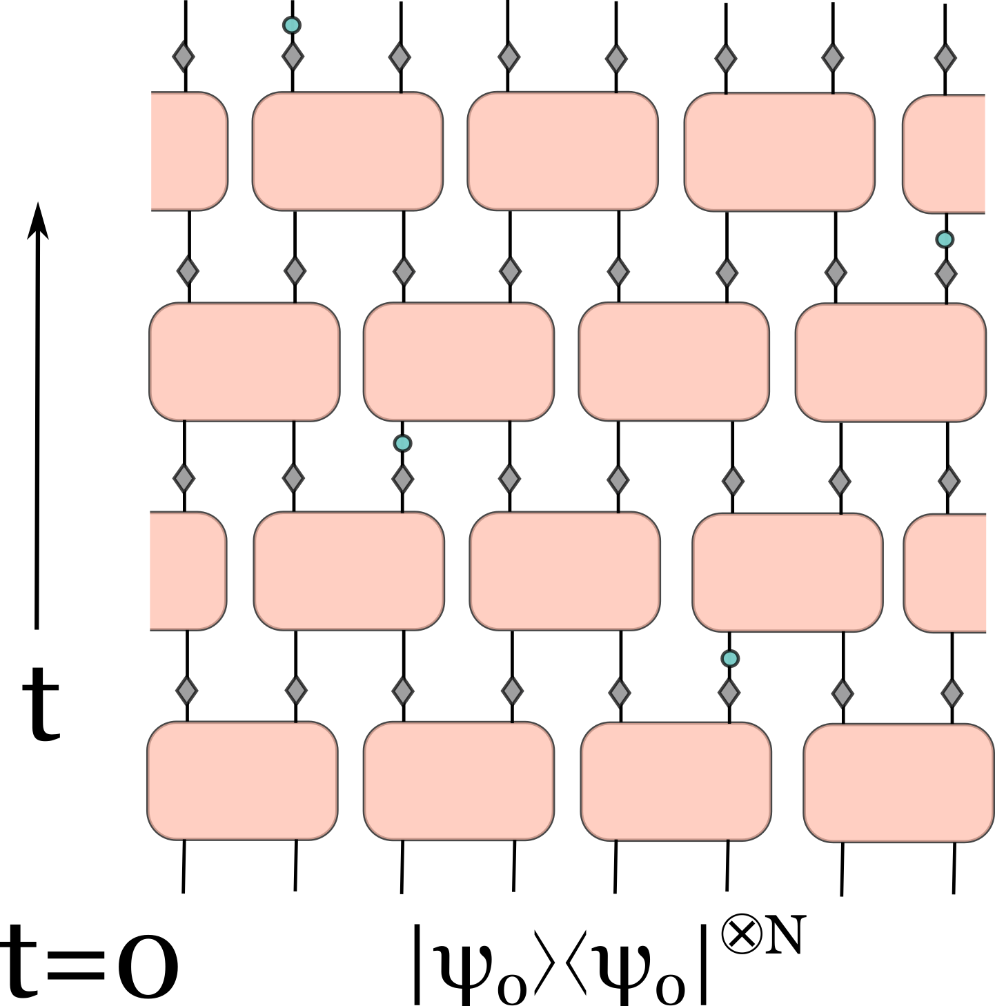
(a)

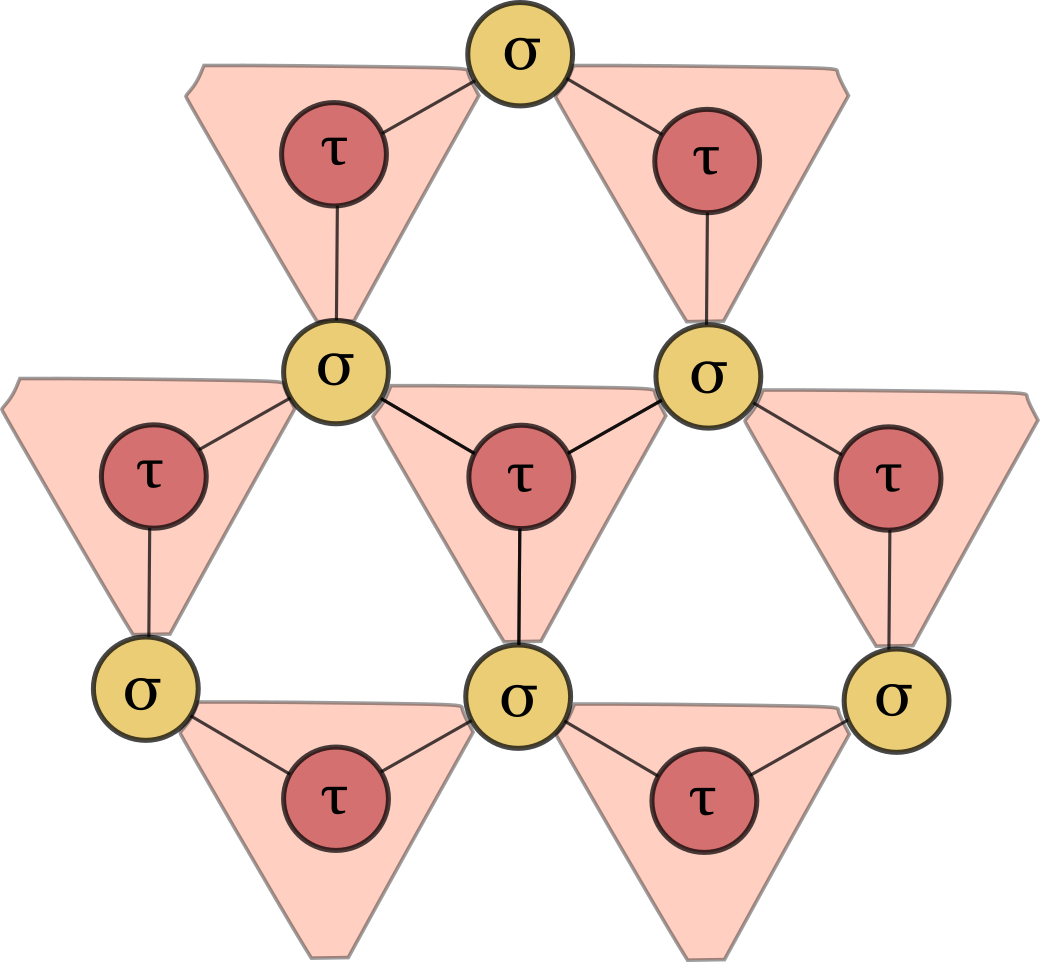
(b)

Figure 1: (a) Brick-wall structure of the random circuits. Each orange rectangle is a 2 qubit random Haar unitary gate. Grey diamonds denote independent dissipation with fixed rate $\Gamma$ and green circles are independent measurement with probability $p$. Ancilla are not shown in this diagram. This structure describes the system dynamics $\rho(t)=\cdots U^{\prime}P\sum_{i}K_{i}U\rho(t_{0})U^{\dagger}K_{i}^{\dagger}PU^{\prime\dagger}\cdots$. (b) The underlying lattice of the classical model that the quantum model is mapped to. The triangular lattice can be obtained using the star-triangle relationship. The time dimension becomes the vertical spatial dimension.

Recently, random quantum circuits (FIG. 1(a)) have been studied extensively due to their tractable representation of a wide range of entanglement phenomena as well as equivalences to other statistical physics problems Li et al. (2019); Li and Fisher (2021); Nahum et al. (2018). Random unitary circuits and driven systems can exhibit extensive entanglement entropy and ballistic information spreading Nahum et al. (2017); Zhou and Nahum (2019); Jonay et al. (2018). The resulting highly entangled state was shown to persist per quantum trajectory even when local monitored measurements are made with a sufficiently small rate, and information remains encoded non-locally. Remarkably, however, a transition from volume law to area law entanglement has been observed upon further increasing the probability of measurement over a critical threshold. This transition is known as the entanglement phase transition or measurement-induced phase transition (MPT), and has been understood in terms of a bond percolation transition through first mapping the $n$-th Rényi entropy to the partition function of an $n!$-state Potts model on a triangular lattice (FIG.1(b)) in the $q\to\infty$ limit, and then taking the replica limit $n\to 1$, where a Potts model turns into a bond percolation problem Lubensky (1983). In the percolation picture, the quantum volume law phase corresponds to the existence of a spanning cluster of the underlying lattice and the area law phase to the lack thereof Li and Fisher (2021); Nahum et al. (2018); Jian et al. (2020).

Realistic implementations of monitored circuits in noisy intermediate-scale quantum (NISQ) devices necessarily involve unwanted interactions with the environment. These can be equivalently regarded as subjecting the qubits to non-unitary quantum channels or Lindbladians, or as monitoring only a subset of measurements while averaging over the rest of the measurement outcomes. The volume-to-area-law transition as a function of monitored measurements disappears in the presence of dissipation Botzung et al. (2021), which can be understood analytically via dissipation explicitly breaking the replica symmetry that needs to be spontaneously broken in the effective classical theory Bao et al. (2020); Weinstein et al. (2022); Li et al. (2023); Nahum et al. (2018); Jian et al. (2021). At the same time, an understanding of the transient entanglement dynamics prior to reaching the long-time steady state remains important, to reveal limitations for time scales and circuit depths for which useful computations can be performed. The coarse grained dynamics of random unitary circuit has been under theoretical scrutiny through the Kardar-Parisi-Zhang equation that describes the surface growth in the effective classical theory Jonay et al. (2018); Nahum et al. (2017); Zhou and Nahum (2019), and how boundary dissipation and bulk probablistic dissipation affect this dynamics is only recently studied in Clifford circuits Weinstein et al. (2022); Liu et al. (2022).

Our work aims to tackle the effect of dissipation in a controlled manner by generalizing the classical statistical mapping of unitary circuits with measurements to include noisy quantum channels. We compute the annealed second Rényi entropy and mutual information by mapping the quantum circuit onto a generalized classical Ising model which includes both biasing magnetic fields and three-spin interactions, and illustrate their emergence for both dephasing and amplitude damping quantum channels. With the circuit initialized in a product state, we then study the mutual information dynamics the effective classical model at finite time with dissipation-induced symmetry-breaking contributions and analyze the dynamical regimes that emerge from domain wall configurations. We then compare the classical behavior with quantum simulations for small systems of qubits subjected to the joint action of recorded measurements and dissipation to an environment.

The rest of the paper is organized as follows: In section II, we introduce the setup of the ancilla-assisted dissipative plus measurement circuit. This overviews a few different representations of quantum operations, where the Lindbladian describes continuous dissipation in realistic devices, the ancilla assisted picture is instrumental in our analytical mapping, and the operator-sum representation is implemented numerically to simulate the open circuit. In section III, we map the second Rényi entropy of two open circuits - dephasing and amplitude damping - to the partition function of a generalized Ising model. We study the relation between the quantum parameters and classical parameters, the former of which consists of the local Hilbert space dimension $q$, the probability of measurement $p$, the dissipation rate $\Gamma$, and the latter of which includes the external field $h$, diagonal pair-wise bonds $J_{13}$ and $J_{23}$, the horizontal pair-wise bond $J_{12}$ and the three-body interaction $J_{123}$. With the classical picture in mind, we obtain the energy-minimizing domain wall configurations from which two dynamical scales of entanglement arise for a finite system, the ballistic growth in a short time, and the exponential decay that follows. We propose a modified classical picture for the dissipative system in the thermodynamic limit, where the time scales do not depend on the system size. In section IV, we simulate the hybrid circuit with on-site amplitude damping and present the short-time dynamics and the steady state values of the mutual information, which confirms qualitatively the intuition and prediction of our classical theory on the 2nd Rényi mutual information of the quantum system. Finally, we comment on possible future directions in section V.

II Setup

The model consists of a chain of $N$ qudits initialized in a product state $\rho(t_{0})=\outerproduct{\psi_{0}}{\psi_{0}}^{\otimes N}=\frac{1}{N}(\sum_{i,j=0}^{q-1}\outerproduct{i}{j})^{\otimes N}$, which is subjected to 2-qudit Haar random unitary gates $U$ that entangle every other pair of neighboring spins. A 2-qubit Haar operator is a matrix drawn uniformly over the unitary group $U(q^{2})$.

After being subjected to a random unitary gate, each qudit interacts with its environment independently at each site. The operator-sum representation of this step is defined via the Kraus operators $\{K_{i}\}$:

$$\rho(t_{0}+\Delta t)=\sum_{i}K_{i}\rho(t_{0})K_{i}^{\dagger}.$$ (1)

The Kraus operators considered in this work can also be described by the Lindbladian evolution by integrating the following equation for finite time $\Delta t$:

$$\dot{\rho}=\gamma\left(\sum_{i}-\frac{1}{2}\{L_{i}L_{i}^{\dagger},\rho\}+L_{i}\rho L_{i}^{\dagger}\right)$$ (2)

where $\gamma$ is the dissipation rate, and $L_{i}$ are the jump operators. The Lindbladian assumes Markovian dissipation, with a vanishing correlation time for the bath. These two equivalent descriptions (1) and (2) of completely positive trace-preserving channels Breuer and Petruccione (2007) can be transformed into each other through the Choi-Jamikolski isomorphism Milz et al. (2017). We henceforth parameterize the dissipation rate via a dimensionless parameter $\Gamma$ for the Kraus operators, which can be equivalently expressed as a function of $\gamma\Delta t$ for a Lindbladian evolving the quantum state over a discrete time step $\Delta t$.

In this work, we consider two dissipation mechanisms: dephasing and amplitude damping. Dephasing can be viewed as an infinite-temperature bath that acts on the system qudits, with Kraus operators

$$K_{0} =\cos(\theta)\mathbb{I},$$

$$K_{i} =\sin(\theta)\sqrt{\frac{q}{2(q-1)}}\gamma_{i},~{}~{}i=1,\dots,q-1.$$

where $\gamma_{i}$ are the diagonal generalized Gell-Mann matrices for qudits $q$, and $[q\cos^{2}(\theta)-1]/2=1-\Gamma q$ determines $\theta$. For qubits, $q=2$, and the corresponding Lindbladian jump operator is the Pauli matrix $\sigma_{z}$, with $\Gamma=(1-e^{-2\gamma\Delta t})/2$. As the jump operator is Hermitian, the density matrix of the system is subjected to sequences of random unitary evolution and the dephasing channel will evolve to a fully mixed state. The derivation of the Kraus operators is included in Appendix A.

The amplitude damping channel is described by a set of Kraus operators

$$K_{0} =\outerproduct{0}{0}+\sqrt{1-\Gamma}\sum_{i=1}^{q-1}\outerproduct{i}{i}$$

$$K_{i} =\sqrt{\Gamma}\outerproduct{i-1}{i},~{}~{}i=1,\dots,q-1.$$

In the amplitude damping channel, the bath can be understood as a zero-temperature environment that absorbs the energy carried by photons emitted from the qudits relaxing to state $\left|0\right>$, or equally as a fully polarized bath of qudits. The corresponding Lindblad jump operator for $q=2$ is $\sigma_{-}=\frac{1}{2}(\sigma_{x}-i\sigma_{y})$. In contrast to the dephasing channel, the steady state of the Lindbladian is pure and fully polarized. Therefore, it reaches a non-trivial mixed state under joint unitary evolution and dissipation even in the absence of measurements.

Yet another description of the open system is to introduce an ancilla that is always initialized at some fixed state $\ket{0}$ and interacts with the principal system through an interaction Hamiltonian that reproduces the dissipative dynamics after tracing out the ancilla

$$\rho(t_{0}+\Delta t)=\Tr_{E}\left(U_{\alpha}\rho(t_{0})\otimes\outerproduct{0}{0}U_{\alpha}^{\dagger}\right),$$ (3)

where $U(t)\equiv U_{\alpha}=e^{iH_{\alpha}}$ describes the interaction with the environment. For example, the unitary evolution for the amplitude damping channel is generated by $H_{\alpha}=\alpha(\sigma_{+}^{S}\sigma_{-}^{E}+\sigma_{-}^{S}\sigma_{+}^{E})$, where $\sigma_{\pm}$ are the raising/lowering operators for qudits. One can then see that the dissipation rate is $\Gamma=\sin^{2}{\alpha}$. This will be the primary example of dissipation considered in this manuscript.

After dissipation, the measurement of each spin in the z-direction is performed with probability $p$ independently, and the probability of an outcome is assigned according to the Born rule, $p_{q}=\frac{P_{m,q}\rho P_{m,q}}{\Tr{P_{m,q}\rho P_{m,q}}}$, where $P_{m,q}$ are projection operator on to the $q$ orthogonal states on the site $m$. The unitary-dissipation-measurement process completes one discrete time step. The next layer consists of the same procedure with Haar random unitaries shifted by one site to create the brickwork pattern in Fig. 1(a). Iterating this procedure creates an ensemble of mixed steady states with different histories of the quenched unitary $U$, the location of measurements, and measurement outcomes, distributed according to the unitary group, the probability $p$, and the Born rule respectively.

III Theory of the transition

The MPT has been understood through a mapping between the entropic measures evaluated for $n$-replicated $(1+1)$ dimensional qudit systems to the partition function $Z$ of the $2$-d classical spin model on a triangular lattice with fixed boundary conditions Bao et al. (2020). Since dissipation is equivalent to measuring and discarding the outcome, introducing dissipation does not change the essence of the mapping, so we will review the mapping here, and extend it to include dissipation.

The primary quantities simulated in prior work are the von Neumann entropy $S(\rho_{A})$ of a subset $A$ of the chain as well as the mutual information $I$ for a bipartition. The von Neumann entropy can be calculated from Rényi entropies of order $n$: $S^{(n)}(\rho_{A})=\frac{1}{1-n}\log\Tr\rho_{A}^{n}$ in the limit $n\to 1$. This quantity can be related to the partition function $Z^{(n)}$ of the $n!$-state Potts model in the $q\to\infty$ limit, so in the $n\to 1$ limit, the entanglement entropy can be understood in terms of bond-percolation or the Fortuin-Kasteleyn random cluster model Lubensky (1983). In random unitary circuits without the $q\to\infty$ and $n\to 1$ limit, a $S_{n}\times S_{n}\rtimes\mathbb{Z}^{\mathbb{H}}_{2}$ symmetry emerges from the replica theory and is spontaneously broken Bao et al. (2021). The classical spin value determines the different ways of connecting the $n$ replicas at every site, and a microstate in the spin system constitutes one complete history of the replicated qudit chain.

The replica limit $n\to 1$ is crucial in producing the correct universality class of the measurement induced phase transition. Nevertheless, the free energy of the Ising model can still illuminate the new type of entanglement dynamics present in a dissipative monitored circuit, analogous to analyses without the replica limit inWeinstein et al. (2022); Bao et al. (2021). To capture entanglement, we compute the annealed Rényi mutual information. Although it is a classical information measure, it reveals quantum correlations as the total thermal entropy is subtracted. Beyond mutual information, deciding the separability of a mixed state is an NP-hard problem Gurvits (2003). Common measures for mixed state entanglement are the negativity or the logarithmic negativityVidal and Werner (2002). However, computing the negativity of the state requires more than two classical states per site, i.e. more than two replicas. This can be done in principle and will be simplified in $q\to\infty$ limit, see Appendix B. Empirically, the dynamics and the steady state values of mutual information and negativity are almost identical [see Appendix C], which also validates entanglement dynamics predicted from the analytic calculation of the mutual information.

In the rest of the section, we will first review how to compute the Rényi entropy of the random circuit of qudits in which the dissipation is in the form of the dephasing channel, by mapping it to an effective spin model. The only difference between the measurement and the dephasing channel here is that after the ancilla and the on-site qudits are coupled completely, the ancilla is projected when a measurement is performed and traced out while the system dissipates. Then we compute the second Rényi entropy of the amplitude damping channel using the Kraus operator representation. Compared to hybrid unitary circuits, the circuit with dissipation can be mapped to an Ising model with general three-body interactions on downward pointing triangles of the resulting triangular lattice, beyond the purview of exact solutions Eggarter (1975). This mapping is exact when $n=2$, but note that for $n\geq 3$ positivity of the classical Boltzmann weights cannot be guaranteed. We then directly use the Boltzmann weights to compute possible domain wall configurations in different time regimes of the quantum system, which translates to the vertical extent of the corresponding 2D classical magnet. We finally estimate the dynamical time scales of the second Rényi mutual information for transitions between different domain wall configurations in finite system size $N$.

III.1 The dephasing channel

The open quantum circuit contains a qudit chain with $q$ states $\{\ket{1},\ket{2},\cdots,\ket{q}\}$ on each site and 2-qudit Haar random unitary matrices $U\in U(q^{2})$ that act on neighboring spins as the orange boxes in Fig. 1(a). The average of the von Neumann entropy Nielsen and Chuang (2010) over the Haar measure is simply

$$\mathbb{E}_{U}[S_{A}] =-\int_{U}dU\Tr{\rho_{A}(U)\log{\rho_{A}(U)}}$$

$$=\frac{\partial}{\partial n}\Big{|}_{n\to 1^{+}}\log\mathbb{E}_{U}[\Tr(\rho^{n})].$$ (4)

The right hand side is not a properly quenched averaged $n$-th Rényi entropy over the Haar ensemble but can be viewed as an annealed Rényi entropy. In this paper, the “Rényi index” is conflated with the number of replicas, i.e. the $n\to 1$ limit will indeed give the von Neumann entropy, but without taking the limit, it does not give a properly averaged $n$-th Rényi entropy, but an “annealed” version of the entropy-like quantity, and is lower bounded by the $n$-th Rényi entropy. For simplicity, it will be referred to it as the $n$-th Rényi entropy and it should be understood that all analytic averaging stays annealed in the replica formalism until $n\to 1$ is taken. There is another similar line of replica calculation where the Rényi index and the number of replicas are independent Weinstein et al. (2022); Jian et al. (2020). One can take both limits at once to obtain the von Neumann entropy, or only the replica limit to obtain the Rényi entropies.

The unitary evolution acting on the replicas will be a tensor product of $n$ Haar matrices $U\in U(q^{2})$, i.e. $U\otimes U^{\dagger}\otimes\cdots\otimes U^{\dagger}$, and averaging over the Haar ensemble results Collins (2003) in a simpler network that hosts only $n!$ degrees of freedom for each $\sigma$ and $\tau\in S_{n}$ on each site

$$\int_{U^{\bigotimes n}}\bigotimes_{i=1}^{n}dU_{i}\;\vbox{\hbox{\includegraphics[scale={0.8}]{diagrams/singlesiteU.png}}}$$

$$=\sum_{\sigma,\tau\in S_{n}}w_{g}(\sigma\tau^{-1},q^{2})\vbox{\hbox{\includegraphics[scale={0.8}]{diagrams/singlesiteSpin.png}}}$$ (5)

where $w_{g}(\sigma\tau^{-1},q^{2})$ is the Weingarten function, which bridges the group of unitary matrices of size $d\times d$ and the symmetric group on $q$ letters $S_{q}$. It is a polynomial function of $d$ of most degree $q$, defined over $S_{q}$ as

$$w_{g}(\sigma,d)=\frac{1}{q!^{2}}\sum_{\lambda}\frac{\chi^{\lambda}(\mathbb{I})^{2}\chi^{\lambda}(\sigma)}{s_{\lambda,d}(\mathbb{I})},$$ (6)

where $\sigma\in S_{n}$, $\lambda$ is a partition, $\chi^{\lambda}$ is the character of the partition, and $s_{\lambda,d}$ is the dimension of the irreducible representation of the unitary group associated with $\lambda$ Collins (2003). In the quantum model, the values of $\sigma$ and $\tau$ represent different configurations of how the replica indices are connected locally. In the classical picture, they are simply the different spin states in the group $S_{n}$. The unitary evolution is followed by dissipation. We choose here an ancilla representation where every qudit on the principal Hilbert space is entangled with an ancilla initialized at $\ket{0}$. The ancilla lives in a Hilbert space of $q+1$ states $\{\ket{0},\ket{1},\cdots\ket{q}\}$ and becomes entangled via the unitary gate $R_{\alpha}=\sum_{i=1}^{q}\outerproduct{i}{i}\otimes e^{-i\alpha X_{i}}$ where $X_{i}=\outerproduct{i}{0}+\outerproduct{0}{i}$. The strength of the interaction is controlled by the dimensionless parameter $\Gamma=\sin^{2}{\alpha}$ Bao et al. (2020). After the application of $R_{\alpha}$, the ancilla degrees of freedom are traced out independently at every site. Tracing out the environment is averaging the state of the principal system over the ensemble of measurement outcomes, which is a simple statistical averaging and requires no replica trick.

The measurement step is operationally similar to but fundamentally different from dissipation. The ancilla gets projected onto its computational basis $\ket{i}_{m}$ (with each basis state describing a trajectory) which can be carried out by $\mathcal{N}_{\phi}[\rho]=\sum_{i=0}^{q}\outerproduct{i}{i}_{m}\rho\outerproduct{i}{i}_{m}$. The von Neumann entropy of the subsystem $A$ can therefore be formally computed as the annealed conditional entropy between the system $M$ and $A$ Bao et al. (2020):

$$\mathbb{E}_{U}[S_{A}] =\frac{\partial}{\partial n}\bigg{|}_{n\to 1^{+}}S^{(n)}_{A}$$ (7)

where

$$S^{(n)}_{A}=\tilde{S}_{AM}^{(n)}-\tilde{S}_{M}^{(n)}$$ (8)

is the difference between the Rényi entropies of the subsystems $AM$ and $M$ after the ancilla are projected onto the trajectory specified by $m$:

$$\tilde{S}_{X}^{(n)}=\log\mathbb{E}_{U}\Tr\{\mathcal{N}_{\phi}[\rho_{X}]^{n}\}.$$ (9)

The average von Neumann entropy $\langle S_{A}\rangle$ is recovered only when $n\to 1$. However, the $S^{(n)}_{A}$ is substantially simpler to compute for fixed $n$. As we are interested in the understanding qualitative features of for small-system dynamics, we focus on calculating $S^{(2)}_{A}$ as well as a corresponding generalized mutual information measure, and compare results to small-system quantum simulations.

III.2 Dephasing channel

Combining the above steps, the effect of dissipation followed by measurement can be compactly expressed by the Boltzmann weight of the diagonal bond of the resulting honeycomb lattice of classical effective spins, by contracting the tensor formed by the diagonal bonds with the tensor formed by the two connected spins $\sigma$ and $\tau$:

$$w^{(n)}_{d}(\sigma,\tau)=\sum_{\vec{a},\vec{b},\vec{a^{\prime}},\vec{b^{\prime}}}\vbox{\hbox{\includegraphics[scale={0.7}]{diagrams/singlesiteMsm.png}}}$$

$$= \sum_{\vec{a},\vec{b},\vec{a^{\prime}},\vec{b^{\prime}}}M^{(n)}_{\vec{a}\vec{b},\vec{a^{\prime}}\vec{b^{\prime}}}\sigma_{\vec{a}\vec{b}}\tau_{\vec{a^{\prime}}\vec{b^{\prime}}}$$

$$= \sum_{\vec{a},\vec{b},\vec{a^{\prime}},\vec{b^{\prime}}}\prod_{k=1}^{n}\Tr\{\mathcal{N}_{\phi}\left[e^{-i\beta X_{a_{k}}}\outerproduct{0}{0}e^{i\beta X_{b_{k}}^{\dagger}}\right]$$

$$\hskip 14.22636pt\delta_{a_{k},a^{\prime}_{k}}\delta_{b_{k},b^{\prime}_{k}}((1-\Gamma)+\delta_{a^{\prime}_{k}b^{\prime}_{k}}\Gamma)\Big{\}}\sigma_{\vec{a}\vec{b}}\tau_{\vec{a^{\prime}}\vec{b^{\prime}}}$$

$$= \sum_{\vec{a},\vec{b}}\Bigg{\{}(1-p)^{n}\prod_{k=1}^{n}\left((1-\Gamma)+\delta_{a^{\prime}_{k}b^{\prime}_{k}}\Gamma\right)$$

$$\hskip 14.22636pt+p^{n}\prod_{k=1}^{n}\delta_{a_{k}b_{k}}\delta_{b_{k}a_{k+1}}\left((1-\Gamma)+\delta_{a^{\prime}_{k}b^{\prime}_{k}}\Gamma\right)\Bigg{\}}\sigma_{\vec{a}\vec{b}}\tau_{\vec{a}\vec{b}}$$

$$= qp^{n}+(1-p)^{n}\times$$

$$\sum_{\vec{a},\vec{b}}\sum_{k=0}^{n-1}(1-\Gamma)^{k}\Gamma^{n-k}q^{\mathrm{\#conn}(\prod_{j}\delta_{a_{j}b_{\sigma}(j)}\delta_{a_{j}b_{\tau}(j)}\prod_{\alpha}^{n-k}\delta_{a_{j_{\alpha}}b_{j_{\alpha}}})}$$

$$= qp^{n}+q^{\mathrm{\#cycle}(\sigma\tau^{-1})}(1-p)^{n}(1-\Gamma)^{n}+(1-p)^{n}\times$$

$$\sum_{\vec{a},\vec{b}}\sum_{k=0}^{n-1}(1-\Gamma)^{k}\Gamma^{n-k}q^{\mathrm{\#conn}(\prod_{j=0}^{n-1}\delta_{a_{j}b_{\sigma}(j)}\delta_{a_{j}b_{\tau}(j)}\prod_{\alpha}^{n-k}\delta_{a_{\alpha}b_{\alpha}})}.$$ (10)

where $\#$conn($\cdot$) is the function that counts the number of connected components of the argument and $\#$cycle($\cdot$) counts the number of cycles of the argument. For example, fix $n=2$, $\sigma=\tau=(12)$. The exponent of $q$ in the $k=1$ term is $\#\text{conn}(\prod_{j=0}^{2-1}\delta_{a_{j}b_{\sigma(j)}}\delta_{a_{j}b_{\tau}(j)}\prod_{\alpha=0}^{2-1}\delta_{a_{j_{\alpha}}b_{j_{\alpha}}}=\#\text{conn}(\delta_{a_{0}b_{1}}\delta_{a_{1}b_{0}}\delta_{a_{0}b_{0}}\delta_{a_{1}b_{1}})=1$. Without the $\prod_{\alpha}^{n-k}\delta_{a_{\alpha}b_{\alpha}}$ term, the connected components are the same as the number of cycles, which would be 2. The cycle structure only depends on $\sigma\tau^{-1}$ which has $S_{n}\times S_{n}$ symmetry, while the connected component depends on $\sigma$ and $\tau$ independently and there is no apparent symmetry associated with the counting of fixed points of $\sigma\tau^{-1}$. This is the replica symmetry breaking that leads to the disappearance of MPT in dissipative systems Bao et al. (2020); Weinstein et al. (2022). The tensor notation is adopted from the previous workBao et al. (2020). In the tensor network picture, the $\alpha$ gates connect all the legs between $\tau$ and $\sigma$, which makes up one connected component, and there are no more cycles. Naturally, the permutations with more fixed points, or more cycles of length 1, will have more connected components. Since the identity $\mathbb{I}\in S_{n}$ fixes every index, its Boltzmann weight is larger than any other spin value and the spin symmetry is broken. When $\Gamma=0$, the third term in (10) drops out and the expression again only depends on the cycle structure of $\sigma\tau^{-1}$, restoring the symmetry.

Because the weights from the Weingarten function can be negative, an extra step must be taken to ensure that the statistical model is sensible. Half of the spins can be summed first, resulting in a spin model defined on a triangular plaquette, such as the one in FIG.1(b). With dissipation, integrating out $\tau$ or $\sigma$ first can in principle, yield distinct magnetic models for the remaining spin $\sigma$ or $\tau$, respectively, while representing the same quantum behavior. We choose the former, with the Boltzmann weight of a triangular plaquette given by

$$w^{(n)}(\sigma_{1},\sigma_{2},\sigma_{3}) =\sum_{\tau\in S_{n}}\vbox{\hbox{\includegraphics[scale={0.8}]{diagrams/threeSpinWeight.png}}}$$

$$=\sum_{\tau\in S_{n}}w_{g}(\sigma_{3}\tau^{-1},q^{2})w_{d}(\sigma_{1},\tau)w_{d}(\sigma_{2},\tau).$$ (11)

This is the star-triangle relation. The 3-body weight is always positive for $n=2$ and positive under certain conditions on $p$ and $q$ for general $n\geq 3$ Bao et al. (2020).

The last step that completes the mapping is to impose the correct boundary condition. The qudit chain is initialized the same way at every site and across different replicas, which means that the bottom boundary of the classical is open and its Boltzmann weight $w_{\text{bottom}}$ is 1. The boundary condition at the top is determined by the subregion $A$ for which the entropy is computed. Recall that the quantities of interest are $\tilde{S}_{AM}^{(n)}$ and $\tilde{S}_{M}^{(n)}$ after (5) and (7) are combined. The former has the subregion $B$ traced out before replicating, while the latter has both $A$ and $B$ traced out before replicating. To write $S$ as a linear function of the replicated density matrix so that it can be substituted into the replica trick in (4), one can insert $\mathbb{I}\in S_{n}$ in the subregion that needs to be traced out first, and insert $C^{(n)}\in S_{n}$ in the subregion where the Rényi entropy needs to be computed. The first term in (7) can be identified with the partition function

$$\mathbb{E}_{U}[\langle\Tr{\rho^{(n)}_{AM}}\rangle]=\mathbb{E}_{U}\Big{[}\Tr\{(\mathcal{C}^{(n)}_{A}\otimes\mathbb{I}^{(n)}_{B}\otimes\mathcal{C}^{(n)}_{M})$$

$$\hskip 56.9055pt\langle\rho(U)_{1}\otimes\cdots\otimes\rho(U)_{n}\rangle\Big{\}}\Big{]}$$

$$= w_{\mathrm{top}}(C^{(n)}_{A},\mathbb{I}^{(n)}_{B},C^{(n)}_{M})\sum_{\{\vec{\sigma}\}}\prod_{i}w^{n}_{3}(\{\sigma^{i}_{1},\sigma^{i}_{2},\sigma^{i}_{3}\})$$

$$= Z^{(n)}_{AM},$$ (12)

where the subscripts of the partition function $Z$ means the spins in the $AM$ subregion of the boundary are pinned in a different direction from those in $B$, which are in the $\mathbb{I}\in S_{n}$ direction. For instance, when $n=2$, all the spins in the subregion $AM$ point down and the spins in the subregion $B$ point up, by convention. Therefore, combining (4), (7), (12), one can compute the von Neumann entropy (7) as the free energy difference between two spin models with different boundary conditions:

$$\mathbb{E}_{U}[\langle S_{A}\rangle] =\frac{\partial}{\partial n}\big{|}_{n\to 1^{+}}\left[\log Z^{(n)}_{AM}-\log Z^{(n)}_{M}\right]$$

$$=\lim_{n\to 1}\frac{1}{n-1}\left[F^{(n)}_{AM,}-F^{(n)}_{M}\right],$$ (13)

The limit is difficult to take as it requires a general expression of the right hand side as a function of $n$. In the confined phase, which is the low-temperature limit of the classical model with the $S_{n}\times S_{n}\rtimes Z^{\mathbb{H}}_{2}$ symmetry, the mixed boundary condition induces at least one domain wall and the entropy hence becomes directly associated to the free energy of the domain wall. In graph theory, this domain wall is a minimal-cut surface in the graph with edges weighted by $w_{g}$ and $w_{d}$, and its existence in the tensor network construction of AdS/CFT gives a means to calculating the von Neumann entropy of the boundary subregion homologous to this surface Ryu and Takayanagi (2006); Pastawski et al. (2015).

For a mixed state, the mutual information $I=S_{A}+S_{B}-S_{AB}$ between subystems $A$ and $B$ provides a measure for quantum correlations in the system. As the limit $n\to 1$ is analytically challenging, we focus on $\tilde{S}_{X}^{(2)}$ as discussed above, which gives the annealed second Rényi mutual information:

$$\tilde{I}^{(2)}_{A:B} :=S^{(2)}_{A}+S^{(2)}_{B}-S^{(2)}_{AB}$$

$$=\tilde{S}_{AM}^{(2)}-\tilde{S}_{M}^{(2)}+\tilde{S}_{BM}^{(2)}-\tilde{S}_{M}^{(2)}-\left(\tilde{S}_{ABM}^{(2)}+\tilde{S}_{M}^{(2)}\right)$$

$$:=F^{(2)}_{A}+F^{(2)}_{B}-\left(F^{(2)}_{AB}+F^{(2)}_{\emptyset}\right).$$ (14)

The numerics has shown that the critical exponents and the critical probability of measurement do not depend on the Rényi index Skinner et al. (2019). The calculation, therefore, simplifies to approximating the free energies of the Ising model $F_{X}\equiv\tilde{S}_{X}^{(2)}$ as a function of the quantum parameters in different limits of the system size and time, for different boundary conditions that are determined by $X$. We take $A$ and $B$ to be bipartitions of the top boundary of the statistical model and the subregion $M$ does not need to appear since it is fixed in the direction $\mathbb{I}\in S_{n}$ in every term. Furthermore, $F_{\emptyset}=S^{(n)}_{M}$ represents the spin model with the entire top boundary fixed to be $\mathbb{I}\in S_{n}$. This term is necessary to compute the conditional entropy and it functions as a constant shift in the mutual information. We note that the Rényi entropies and its generalized annealed versions do not satisfy subadditivity, so the corresponding mutual information can be negative Scalet et al. (2021). Alternative generalizations of mutual information have been proposed such as the Petz Rényi mutual information or the Rényi divergence Scalet et al. (2021); Kudler-Flam (2023), the study of which will be left for future work.

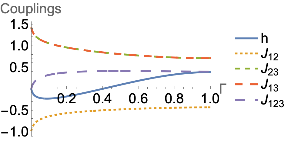
Figure 2: Classical parameters as a function of the parameters in the quantum model, with $p=0.1,q=2$.

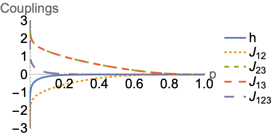
Figure 3: Classical parameters as a function of the parameters in the quantum model, with $\Gamma=0.001,q=2$.

With the boundary conditions established, we are now ready to map the twice-replicated open quantum circuit ($n=2$) above to the Ising spins defined the downward pointing triangular plaquette with arbitrary interactions. The Boltzmann weight on one plaquette is:

$$w(\sigma_{1},\sigma_{2},\sigma_{3})=e^{-\beta E(\sigma_{1},\sigma_{2},\sigma_{3})}$$

$$:=\exp\{h_{0}+h_{1}\sigma_{1}+h_{2}\sigma_{2}+h_{3}\sigma_{3}+J_{12}\sigma_{1}\sigma_{2}$$

$$\hskip 28.45274pt+J_{23}\sigma_{2}\sigma_{3}+J_{31}\sigma_{3}\sigma_{1}+J_{123}\sigma_{1}\sigma_{2}\sigma_{3}\big{\}},$$ (15)

Here, $J_{123}$ is the coupling between the three spins for a downward-facing triangle, the $J_{ij}$ are the pairwise couplings, $h_{i}$ describe effective external magnetic fields, and $h_{0}$ is a normalization. Each of these effective parameters depends on the measurement and dissipation rates $p$ and $\Gamma$, as well as the qudit dimension $q$. All eight parameters are defined via the weights for eight distinct configurations of triangle spins $w(\sigma_{1},\sigma_{2},\sigma_{3})$, where $\sigma_{1},\sigma_{2}$, and $\sigma_{3}$ are taken to denote the top left, top right and bottom spin of downward-pointing triangles. Combining the triangles into a triangular-lattice Ising model, the total magnetic field acting on each spin is $h=\sum_{i=1}^{3}h_{i}$ because every lattice spin is at the corner of three downward triangles.

We illustrate how the classical parameters behave as one adjusts the quantum parameters $\Gamma$ and $p$ respectively in FIG.2 and FIG. 3. In the absence of dissipation, all the symmetry-breaking terms $h_{i}$ and $J_{123}$ are 0, which recovers the spin model in Bao et al. (2020). Increasing the probability of measurement $p$ weakens pairwise interactions, eventually reaching a transition from ferromagnetic order to disorder. When $\Gamma>0$, the symmetry-breaking terms $h_{i}$ and $J_{123}$ become non-zero, and the probability of measurement $p$ decreases bias terms at a much faster rate than the pairwise interaction couplings (FIG.3). We will see similar effects of $p$ and $\Gamma$ for the amplitude damping channel in the next subsection.

III.3 Amplitude damping channel

Now consider the amplitude damping channel. The reader who only wishes to know the consequence of the calculation, i.e. the entanglement dynamics described by the domain walls rather than the details of using of replica symmetry breaking tensor diagrams, can skip to section III.4. This channel is commonly used to model spontaneous emission processes, e.g., the qudit chain is coupled to a polarized zero-temperature bath, which forces the system qudits to collapse to $\ket{0}$. The Kraus operators for the channel are $\{K_{0}=\outerproduct{0}{0}+\sqrt{1-\Gamma}\sum_{i=1}^{q-1}\outerproduct{i}{i},K_{m}=\sqrt{\Gamma}\outerproduct{m-1}{m}\}_{m=1}^{q-1}$. To introduce these to the mapping, we replace the ancilla couplings ($\alpha$ gates) by a sum over Kraus operators. The weights are computed from contracting $\sum_{m=0}^{q-1}K_{m,a^{\prime}_{i}a_{i}}K^{\dagger}_{m,b^{\prime}_{i}b_{i}}$, $i=1,\dots,n$ with the $\sigma$ and $\tau$ tensors, weighted by the same coupling to the measurement ancillae. One obtains the following:

$$w^{(n)}_{d}(\sigma,\tau)=\sum_{\vec{a},\vec{b},\vec{a^{\prime}},\vec{b^{\prime}}}\vbox{\hbox{\includegraphics[scale={0.8}]{diagrams/singlesiteKraus.png}}}$$

$$=\sum_{\vec{a},\vec{b},\vec{a^{\prime}},\vec{b^{\prime}}}\prod_{j=1}^{n}\Big{[}(\delta_{a^{\prime}_{j}0}\delta_{a_{j}0}+\sqrt{1-\Gamma}(\delta_{a^{\prime}_{j}a_{j}}-\delta_{a^{\prime}_{j}0}\delta_{a_{j}0}))(\delta_{b^{\prime}_{j}0}\delta_{b_{j}0}+\sqrt{1-\Gamma}(\delta_{b^{\prime}_{j}b_{j}}-\delta_{b^{\prime}_{j}0}\delta_{b_{j}0}))$$

$$\hskip 28.45274pt+\Gamma\sum_{m=1}^{q}\delta_{a^{\prime}_{j}m-1}\delta_{a_{j}m}\delta_{b^{\prime}_{j}m}\delta_{b_{j}m-1}\Big{]}\Big{[}(1-p)^{n}+p^{n}\prod_{k=1}^{n}\delta_{b^{\prime}_{k}a^{\prime}_{k+1}}\delta_{a^{\prime}_{k}b^{\prime}_{k}}\Big{]}\delta_{a^{\prime}_{j}b^{\prime}_{\sigma(j)}}\delta_{a_{j}b_{\tau(j)}}$$

The first bracket in the product (LABEL:eq:_w_d_of_sigma_-) explicitly breaks the replica symmetry. In the dephasing channel, the identity $\mathbb{I}\in S_{n}$ will give the highest Boltzmann weight because it has the most connected components. In this channel, the same structure is imposed by the $K_{i}$ terms, favoring the configuration $\mathbb{I}$ that maximizes the number of total connections of the delta functions. To simplify the weights from (LABEL:eq:_w_d_of_sigma_-), we create the following diagrammatic rules. The terms from $K_{0}$ has the two following contributions - the stub for $\delta_{a_{i}0}$s and the legs for $\delta_{a_{i}a^{\prime}_{i}}$s:

$$\delta_{a_{i}0}\delta_{b_{i}0}\delta_{a^{\prime}_{i}0}\delta_{b^{\prime}_{i}0} =\vbox{\hbox{\includegraphics[scale={1}]{diagrams/delta_ai_0.png}}},\;$$

$$\sum_{a_{i},a^{\prime}_{i},b_{i},b^{\prime}_{i}}\delta_{a_{i}0}\delta_{b_{i}0}\delta_{a_{i}0}\delta_{b_{i}0} =\vbox{\hbox{\includegraphics[scale={1}]{diagrams/sum_delta_ai_0.png}}}=1$$ (17)

where the stub is contracted with the state $\ket{0}$, which gives the sum 1. The straight legs live in the $(q-1)$ dimensional Hilbert space with the states $\{1,\dots,q-1\}$

$$\delta_{a_{i}a^{\prime}_{i}}\delta_{b_{i}b^{\prime}_{i}}=\vbox{\hbox{\includegraphics[scale={1}]{diagrams/delta_ai_api.png}}};\;\sum_{a_{i},a^{\prime}_{i},b_{i},b^{\prime}_{i}=1}^{q-1}\delta_{a_{i}a^{\prime}_{i}}\delta_{b_{i}b^{\prime}_{i}}\vbox{\hbox{\includegraphics[scale={1}]{diagrams/sum_delta_ai_api.png}}}=q-1.$$ (18)

Each term above is accompanied by a factor of $(1-\Gamma)$. The contraction of (17) and (18) between different replicas yields 0. The tensor and tensor contraction associated with the operator $K_{i}$ is

$$\delta_{a_{i}b_{i}}\delta_{a^{\prime}_{i}b^{\prime}_{i}}\delta_{a_{i}a^{\prime}_{i}-1} =\vbox{\hbox{\includegraphics[scale={1}]{diagrams/delta_ai-1_api.png}}};$$

$$\sum_{a_{i},b_{i}=1}^{q-1}\sum_{a^{\prime}_{i}b^{\prime}_{i}=0}^{q-1}\delta_{a_{i}b_{i}}\delta_{a^{\prime}_{i}b^{\prime}_{i}}\delta_{a_{i}-1a^{\prime}_{i}} =\vbox{\hbox{\includegraphics[scale={1}]{diagrams/sum_delta_ai-1_api.png}}}=q-1,$$ (19)

where the circles with the minus sign ensure that $a^{\prime}_{i}=a_{i}-1$ and $b^{\prime}_{i}=b_{i}-1$. The diagram is always accompanied by $\Gamma$. The upper legs of the circle live in the Hilbert space spanned by $\{\ket{0},\dots,\ket{q-2}\}$ and the lower legs by $\{\ket{1},\dots,\ket{q-1}\}$, both having one fewer dimension than the straight legs from $K_{0}$. This means that in the cross terms, the contraction between the Hilbert space $\{\ket{0},\dots,\ket{q-2}\}$ of $K_{0}$ and $\{\ket{1},\dots,\ket{q-1}\}$ of $K_{i}$ gives $q-2$.

The contractions shown above occur when the output ket $a^{\prime}_{i}$ and bra $b^{\prime}_{i}$ are identified within each replica, i.e. when the spin points in the $\uparrow$ direction. From this, we can calculate the diagrams that contribute to the weight $w(\uparrow\uparrow)$ in the Ising case ($n=2$) as the following:

$$w_{d}(\uparrow\uparrow) =\Bigg{[}\vbox{\hbox{\includegraphics[scale={0.8}]{w_++_/K1_diag1.png}}}+2(1-\Gamma)\vbox{\hbox{\includegraphics[scale={0.8}]{w_++_/K1_diag2.png}}}+(1-\Gamma)^{2}\vbox{\hbox{\includegraphics[scale={0.8}]{w_++_/K1_diag4.png}}}$$

$$+2\Gamma\vbox{\hbox{\includegraphics[scale={0.8}]{w_++_/K1_diag5.png}}}+2\Gamma(1-\Gamma)\vbox{\hbox{\includegraphics[scale={0.8}]{w_++_/K1_diag6.png}}}+\Gamma^{2}\vbox{\hbox{\includegraphics[scale={0.8}]{w_++_/K1_diag7.png}}}\Bigg{]}(1-p)^{2}$$

$$+\Bigg{[}\vbox{\hbox{\includegraphics[scale={0.8}]{w_++_/K1_diag8.png}}}+(1-\Gamma)^{2}\vbox{\hbox{\includegraphics[scale={0.8}]{w_++_/K1_diag9.png}}}+2\Gamma\vbox{\hbox{\includegraphics[scale={0.8}]{w_++_/K1_diag10.png}}}$$

$$+\Gamma^{2}\vbox{\hbox{\includegraphics[scale={0.8}]{w_++_/K1_diag11.png}}}\Bigg{]}p^{2}$$

$$=[1+2(1-\Gamma)(q-1)+(1-\Gamma)^{2}(q-1)^{2}+2\Gamma(q-1)$$

$$+2\Gamma(1-\Gamma)(q-1)^{2}+(q-1)^{2}\Gamma^{2}](1-p)^{2}$$

$$+\big{[}1+(1-\Gamma)^{2}(q-1)+2\Gamma+\Gamma^{2}\big{]}p^{2}$$

$$=q^{2}(1-2p+p^{2})+qp^{2}+2p^{2}\Gamma^{2}.$$ (20)

Factors of 2 are introduced due to the invariance of the tensor contraction under the exchange of the two replicas. When the brakets connect different copies, as a general rule, any connected component contributes a factor of $q-1$, except for those involving a stub (17), which contributes 1, and when the (18) is connected to the upper leg of (19), which contributes $q-2$. The other weights can be derived similarly:

$$w_{d}(\downarrow\downarrow) =\Bigg{[}\vbox{\hbox{\includegraphics[scale={0.8}]{w_--_/K2_diag1.png}}}+(1-\Gamma)^{2}\vbox{\hbox{\includegraphics[scale={0.8}]{w_--_/K2_diag2.png}}}+2(1-\Gamma)\vbox{\hbox{\includegraphics[scale={0.8}]{w_--_/K2_diag3.png}}}$$

$$+\Gamma^{2}\vbox{\hbox{\includegraphics[scale={0.8}]{w_--_/K2_diag4.png}}}\Bigg{]}(1-p)^{2}+\Bigg{[}\vbox{\hbox{\includegraphics[scale={0.8}]{w_--_/K2_diag5.png}}}+(1-\Gamma)^{2}\vbox{\hbox{\includegraphics[scale={0.8}]{w_--_/K2_diag6.png}}}$$

$$+\Gamma^{2}\vbox{\hbox{\includegraphics[scale={0.8}]{w_--_/K2_diag7.png}}}\Bigg{]}p^{2}$$

$$=(q^{2}(1-\Gamma)^{2}+q(2-\Gamma)\Gamma)(1-p)^{2}$$

$$+(1+(q-1)(2\Gamma^{2}-2\Gamma+1))p^{2}$$ (21)

$$w_{d}(\uparrow\downarrow) =\Bigg{[}\vbox{\hbox{\includegraphics[scale={0.8}]{w_+-_/K4_diag1.png}}}+(1-\Gamma)^{2}\vbox{\hbox{\includegraphics[scale={0.8}]{w_+-_/K4_diag2.png}}}$$

$$+2\Gamma(1-\Gamma)\vbox{\hbox{\includegraphics[scale={0.8}]{w_+-_/K4_diag3.png}}}+\Gamma^{2}\vbox{\hbox{\includegraphics[scale={0.8}]{w_+-_/K4_diag4.png}}}\Bigg{]}(1-p)^{2}$$

$$+\Bigg{[}\vbox{\hbox{\includegraphics[scale={0.8}]{w_+-_/K4_diag5.png}}}+\vbox{\hbox{\includegraphics[scale={0.8}]{w_+-_/K4_diag6.png}}}(1-\Gamma)^{2}+\vbox{\hbox{\includegraphics[scale={0.8}]{w_+-_/K4_diag7.png}}}\Gamma^{2}\Bigg{]}p^{2}$$

$$=[1+(q-1)(1-\Gamma)^{2}+(q-1)\Gamma^{2}+2(q+1)\Gamma(1-\Gamma)]$$

$$(1-p)^{2}+[1+(q-1)(1-\Gamma)^{2}+(q-1)\Gamma^{2}]p^{2}$$

$$=q((1-p)^{2}+p^{2}(2\Gamma^{2}-2\Gamma+1))+2p^{2}\Gamma(1-\Gamma)$$ (22)

$$w_{d}(\downarrow\uparrow) =\Bigg{[}\vbox{\hbox{\includegraphics[scale={0.8}]{w_-+_/K3_diag1.png}}}+(1-\Gamma)\vbox{\hbox{\includegraphics[scale={0.8}]{w_-+_/K3_diag2.png}}}+\Gamma^{2}\vbox{\hbox{\includegraphics[scale={0.8}]{w_-+_/K3_diag3.png}}}$$

$$+2\Gamma(1-\Gamma)\vbox{\hbox{\includegraphics[scale={0.8}]{w_-+_/K3_diag4.png}}}+2\Gamma\vbox{\hbox{\includegraphics[scale={0.8}]{w_-+_/K3_diag5.png}}}\Bigg{]}((1-p)^{2}+p^{2})$$

$$=[1+(q-1)(1-\Gamma)^{2}+(q-1)\Gamma^{2}$$

$$+2(q-2)\Gamma(1-\Gamma)](p^{2}+(1-p)^{2})$$

$$=(q+2\Gamma^{2})(1-2p+2p^{2}).$$ (23)

We note that the diagrams illustrate how to generalize the weight computation for general $n>2$, but the positivity of the Boltzmann weights is again not guaranteed.

At small values of $\Gamma$ and $p$, the Ising model representation of the emission channel behaves similarly to the dephasing channel. This can be understood as the principal function of dissipation at small $\Gamma$ is making the quantum state mixed regardless of the specific dissipative mechanism. At small enough $\Gamma$, dissipation increases the biasing terms and decreases pair-wise interactions, as can be seen from FIG.4. As $\Gamma$ increases, the bath ultimately forces the quantum system into a fully polarized state. At very large $\Gamma$, the parameters of the two classical models have very different behaviors, which illustrates that the two steady states, $\frac{1}{N}\mathbb{I}^{\otimes N}$ and $\ket{0}^{\otimes N}$, of the open quantum circuits are drastically different, as a result from interacting with an infinite temperature and zero-temperature bath.

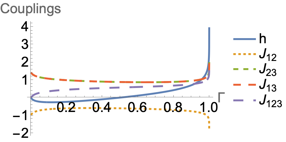
Figure 4: Classical parameters as a function of the parameters in the quantum model in the amplitude damping model, with $p=0.1,q=2$.

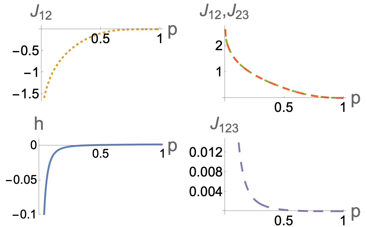
Figure 5: Classical parameters as a function of the parameters in the quantum model in the amplitude damping model, with $\Gamma=0.001,q=2$.

The dependence of the individual couplings on $p$ at $\Gamma=0.001$ are shown in FIG.5. As $p$ increases, the symmetry-breaking $h$ and $J_{123}$ are quickly suppressed to orders of magnitude smaller than $J_{ij}$, which restores the long-range order in the pairwise Ising model on the triangular lattice Bao et al. (2020); Eggarter (1975) and nudges the dissipative system towards larger steady-state entanglement. This suggests sweet spots which, although obeying area laws for mutual information and entanglement negativity, yield maximal prefactors for their asymptotic behavior by virtue of competition between dissipation and measurements. The consequences for the mutual information will be further analyzed in the next section.

III.4 $\tilde{S}^{(n)}_{X}$ and domain walls

We now turn to extract the mutual information $\tilde{I}^{(2)}$ from domain walls that form for different boundary conditions in (14). Without dissipation, the free energy of domain walls scales with the subsystem size $N/2$ in the small-$p$ ferromagnetic phase for $F_{A}$ and $F_{B}$ while $F_{AB}$ and $F_{\emptyset}$ remain trivial, which results in an entanglement volume law.

At finite $\Gamma$, the situation becomes richer: the energy of boundary-enforced domains with spins that are anti-aligned to the bias field and three-spin interaction now scales with the domain area rather than just the domain wall length. The enclosed area is a product of the subsystem size and the time-like direction, and preferable domain wall configurations will therefore sensitively depend on time. Furthermore, $F_{AB}$ can favor hosting domain walls as well. The expected area laws in the steady state must consequently result from the cancellation of free energies from different boundary conditions.

III.4.1 $p=0$ measurement limit, $t\to\infty$

We start by reviewing the limit of an unmonitored circuit at long times and use the exact dependence of the Boltzmann weights on $(p,\Gamma)$ to deduce the saddle point of the classical model with different boundary conditions and in the two-dimensional limit for the classical model, to extract the steady state behavior of the mutual information. This is tractable as there is no entropic contribution to the free energy of the model. At $p=0,\Gamma\neq 0$, the classical system will minimize the area spanned by , because will always cost less energy from FIG.6. Even though domain walls are energetically costly, in the thermodynamic and at long times, the bulk will be fully $\uparrow$ polarized regardless of the boundary condition. All domain walls therefore stick to the top boundary and determine the Rényi mutual information (14). After subtracting a system-spanning domain wall in $F_{AB}$ from two half system domain walls in $F_{A}$ and $F_{B}$, only a contribution from the boundary between subsystems $A$ and $B$ remains. This means that the mutual information obeys an area law, as expected. We carry out the infinite $q$ expansion of the domain wall configuration explicitly in Appendix.B. From table. 1, the leading order of $\frac{1}{q}$ to the Rényi mutual information is:

$$\tilde{I}^{(2)}_{A:B} =F^{(2)}_{A}+F^{(2)}_{B}-(F^{(2)}_{AB}+F^{(2)}_{\emptyset})$$

$$=E(\downarrow\in A,\;\uparrow\in B)+E(\uparrow\in A,\;\downarrow\in B)$$

$$\hskip 28.45274pt-(E(\downarrow\in AB)+E(\uparrow\in AB))$$

$$=F\left(\vbox{\hbox{\includegraphics[scale={0.5}]{diagrams/F_A_bdry.png}}}\right)+F\left(\vbox{\hbox{\includegraphics[scale={0.5}]{diagrams/F_B_bdry.png}}}\right)$$

$$-F\left(\vbox{\hbox{\includegraphics[scale={0.5}]{diagrams/F_AB_bdry.png}}}\right)-\left(\vbox{\hbox{\includegraphics[scale={0.5}]{diagrams/F_empty_bdry.png}}}\right)$$

$$\approx 2\lim_{q\to\infty}\bigg{(}E(\vbox{\hbox{\includegraphics[scale={0.4}]{triangles/pmp.png}}})+E(\vbox{\hbox{\includegraphics[scale={0.4}]{triangles/mpp.png}}})$$

$$\hskip 28.45274pt-E(\vbox{\hbox{\includegraphics[scale={0.4}]{triangles/mmp.png}}})-E(\vbox{\hbox{\includegraphics[scale={0.4}]{triangles/ppp.png}}})\bigg{)}$$

$$=4\log 1=0.$$ (24)

The factor of 2 comes from the periodic boundary condition in the spatial direction of the quantum model. The diagrams in the third line are the classical configurations close to the last time slice of the random circuits (FIG.1(a)) and the dark regions mark the downward spin clusters. The corresponding quantum state is a product state in spite of the infinite number of on-site degrees of freedom, which is expected when the system only scrambles and dissipates, wherein the unitary scrambling accelerates the dissipation since the local information dissipates globally.

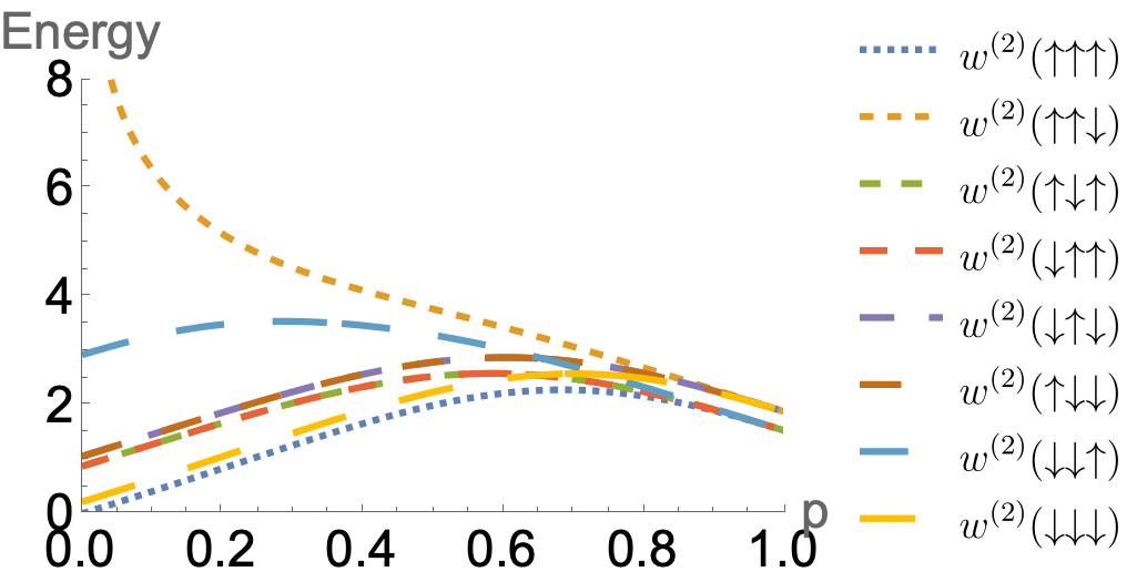
Figure 6: The energy of each plaquette in the Ising model (12) mapped from the dissipative open circuit. $\Gamma$ is set to 0.1 to exaggerate the Ising symmetry breaking in the weights.

When $q<\infty$, the mutual information receives correction in $p$, $\Gamma$ and $\frac{1}{q}$, which turns out to be negative. This is not prohibited because Rényi entropies do not satisfy subadditivity. Its negativity is heuristically an extreme case of the “decoupling principle” Li and Fisher (2021); Li et al. (2021), where quantities like $\Tr{\rho_{AB}^{2}}$ may encode more information than $\Tr{\rho_{A}^{2}}$ or $\Tr{\rho_{B}^{2}}$ combined, because the former contains interactions between the subsystem $A$ and $B$. This may especially be true for systems that interact with a bath since measuring the subsystem $A$ reveals “less information about $B$ than 0”, where 0 is the decoupling principle in the $\Gamma\to 0$ limit. The naive Rényi mutual information can be computed in terms of Boltzmann weights of the individual plaquette (FIG.6)

$$\tilde{I}^{(2)}_{A:B}(p=0,q,\Gamma>0)=2\log\left(\frac{w(\uparrow\downarrow\uparrow)w(\downarrow\uparrow\uparrow)}{w(\downarrow\downarrow\uparrow)w(\uparrow\uparrow\uparrow)}\right),$$ (25)

The case $(p=0,\Gamma=0)$ is excluded because in this limit $w(\downarrow\downarrow\uparrow)=w(\uparrow\uparrow\downarrow)=0$, which means the horizontal domain wall costs infinite energy, and the picture breaks down. On the other hand, for $\Gamma=0$, the mutual information will be in the volume law phase because there will be no domain walls for homogeneous boundaries and the energies of and are 0:

$$\tilde{I}^{(2)}_{A:B}(p=0,q,\Gamma=0)$$

$$=F\left(\vbox{\hbox{\includegraphics[scale={0.5}]{diagrams/F_A_tri.png}}}\right)+F\left(\vbox{\hbox{\includegraphics[scale={0.5}]{diagrams/F_B_tri.png}}}\right)$$

$$-F\left(\vbox{\hbox{\includegraphics[scale={0.5}]{diagrams/F_AB_whole.png}}}\right)-F\left(\vbox{\hbox{\includegraphics[scale={0.5}]{diagrams/F_empty_whole.png}}}\right)$$

$$\approx-N\log\left(\frac{w(\uparrow\downarrow\uparrow)w(\downarrow\uparrow\uparrow)}{w(\uparrow\uparrow\uparrow)w(\downarrow\downarrow\downarrow)}\right)$$

$$=-2N\log w(\uparrow\downarrow\uparrow)$$ (26)

where $-2\log w(\uparrow\downarrow\uparrow)$ would be the prefactor of the volume law growth for the mutual information.

III.4.2 $p>0$, $t<t^{*}_{A}$ (short time regime)

Introducing measurements makes the system more entropic, lowering the free energy of the classical model and the entanglement in the quantum model, but the free energy is still dominated by energy ($p<p_{c}$). As seen from section III.3 and FIG.6, the measurement probability $p$ decreases the strength of the bias field and three-spin interactions.

We analyze the domain wall configuration in $F_{A}$ by studying the energetic and entropic contributions of two symmetric random walkers that start from the top ($t=t_{\mathrm{final}}$) $AB$ boundary. First, we eliminate the possibility of a horizontal domain wall because it incurs a high energy cost, as seen from the Boltzmann weights in FIG. 6, and will hence be unstable to the following fluctuation

$$\vbox{\hbox{\includegraphics[scale={0.4}]{diagrams/eg2fluc.png}}}\Rightarrow\vbox{\hbox{\includegraphics[scale={0.4}]{diagrams/eg1fluc.png}} }$$ (27)

as the latter configuration is energetically much cheaper. Therefore, the allowed moves for the walkers will be and at short time scales, which means that the domain wall must connect the top $t=t_{\rm max}$ and bottom ($t=0$) boundaries. Within time $t$, the total number of sample paths is $2^{2t}$. However, not all walks have equal energies, and we estimate the energy of the two parallel walks as it is the most entropic choice amongst the $2^{2t}$ paths while keeping the energy identical, which makes up a macrostate with well-defined free energy. The parallel constraint halves the number of paths, which will underestimate the domain wall fluctuation so the actual entropy of the state is bounded between $2t\log 2$ and $t\log 2$. We therefore denote the entropic correction as $\lambda t$ with $\log(2)\lesssim\lambda\lesssim 2\log(2)$. We note that for much larger $\Gamma$, domain wall configurations must instead minimize the domain area with anti-aligned spins, but we focus here on $\Gamma\ll p<1$. Similarly, $F_{AB}$ and $F_{\emptyset}$ must both remain fully polarized as a horizontal domain for $F_{AB}$ is too costly, and hence increase linearly with time. Collectively, the mutual information grows linearly, which follows from the free energy difference per unit time $\Delta E$ as:

$$\Delta E(p,\Gamma)=-\log{\frac{w(\uparrow\downarrow\uparrow)w(\uparrow\downarrow\downarrow)}{w(\uparrow\uparrow\uparrow)w(\downarrow\downarrow\downarrow)}}$$ (28)

This needs to be corrected by the entropy growth $t\log 2$ per random walker. Therefore, the total mutual information growth reads

$$\tilde{I}^{(2)}_{A:B} =F\left(\vbox{\hbox{\includegraphics[scale={0.5}]{diagrams/F_A_half.png}}}\right)+F\left(\vbox{\hbox{\includegraphics[scale={0.5}]{diagrams/F_B_half.png}}}\right)$$

$$\hskip 14.22636pt-F\left(\vbox{\hbox{\includegraphics[scale={0.5}]{diagrams/F_AB_whole.png}}}\right)-F\left(\vbox{\hbox{\includegraphics[scale={0.5}]{diagrams/F_empty_whole.png}}}\right)$$

$$=2t\Delta E-2\lambda t$$

$$=v_{2}(p,\Gamma)t.$$ (29)

Termed the entanglement velocity Zhou and Nahum (2019), $v_{2}(p,\Gamma)$ is shown in FIG.7 as a function of dissipation and measurement rates for parallel walkers $\lambda=\log(2)$, which shows that they both smoothly slow down the entanglement growth. The growth in free energy here is the same mechanism as the entanglement growth of the Rényi entropy in the case without dissipation, but twice in value. Each Rényi entropy has its own velocity $v_{n}$ that is the prefactor of the ballistic surface growth predicted by the KPZ equation, followed by the subleading correction $t^{1/3}$ that accounts for the fluctuation Li et al. (2021); Li and Fisher (2021); Zhou and Nahum (2019); Weinstein et al. (2022); Liu et al. (2022). A bound on the growth of the mutual information would be difficult to estimate because the speed at which $S^{(n)}_{A}$ and $S^{(n)}_{AB}$ are separately bounded and with opposite signs. In principle, the estimated velocity for Rényi index $n>1$ can be negative at large $p$; however, the above domain wall analysis breaks down for large $p$ as entropy dominates the free energy.

Figure 7: The prefactor of the extensive part of the second Rényi mutual information of the dissipative quantum circuit.

III.4.3 $p>0$, $t^{*}_{A}<t<t^{*}_{AB}$ (intermediate time regime)

For $F_{A}$ and $F_{B}$ at longer times, the pair of domain walls that traverse the time direction will instead transition to one that traverses the spatial direction, i.e. it starts and ends on the same boundary. First, the two random walkers can now cross via low-energy diagonal moves and hence terminate. Second, the domain with spins aligned in the direction disfavored by the symmetry-breaking terms $h$ and $J_{123}$ will be minimized for longer times, making a domain wall that starts and ends on the top boundary energetically favorable.

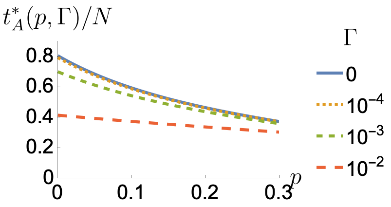
Figure 8: The rescaled crossover times $t^{*}_{A}/N$ for finite system size $N$ (right). The system size used is $N=250$.

When the system size $N$ is sufficiently small, the free energy that includes the entropy $\lambda t$ in the previous subsection is appropriate since $t$ for this configuration can be on the same order as $N$. After $t_{A}^{*}$, a different domain wall configuration for $F_{A}$ can appear, which consists of diagonal domain walls that encloses a V-shaped region of $\downarrow$ like that in $F_{A}(p=0,\Gamma=0)$. Entropic contributions are suppressed as the following fluctuation on the laterals of the triangles

$$\vbox{\hbox{\includegraphics[scale={0.4}]{diagrams/eg3fluc.png}}}\Rightarrow\vbox{\hbox{\includegraphics[scale={0.4}]{diagrams/eg4fluc.png}} }$$ (30)

incurs an enormous energy cost for small $p$ due to substituting by .

Equating the free energies of the short and intermediate-time domain wall states

$$\hskip 28.45274ptF\left(\vbox{\hbox{\includegraphics[scale={0.4}]{diagrams/F_A_half.png}}}\right)=F\left(\vbox{\hbox{\includegraphics[scale={0.4}]{diagrams/F_A_tri.png}}}\right)$$ (31)

defines the time scale $t_{A}^{*}$ via the solution of

$$-t^{*}_{A}\bigg{(}\log w(\uparrow\downarrow\uparrow)w(\uparrow\downarrow\downarrow)+\frac{N-2}{2}\log w(\downarrow\downarrow\downarrow)+\lambda\bigg{)}$$

$$=-\frac{1}{2}\left(\frac{N}{2}-1\right)^{2}\log w(\downarrow\downarrow\downarrow)-N\log w(\downarrow\uparrow\uparrow)$$

$$\hskip 28.45274pt-\bigg{[}\frac{N}{2}t^{*}_{A}-\frac{1}{2}\left(\frac{N}{2}+1\right)^{2}\bigg{]}\log w(\uparrow\uparrow\uparrow)$$ (32)

where only the region where the two saddle points differ is equated in the free energy expression above which consists of $\frac{Nt^{*}_{A}}{2}$ plaquettes; the rest of the state would be uniformly $\uparrow$. The solution of $t^{*}_{A}$ is plotted in FIG.8. This $t^{*}_{A}$ is proportional to the system size $N$. $t^{*}_{A}$ is shortened with increasing $p$ and $\Gamma$. This together with the decrease in the entanglement velocity $v_{2}$ predicted in III.4.2 explains why circuits with higher rate of measurement and dissipation form less entanglement even at short times. We note that in the thermodynamic limit $N\to\infty$ as well as in the large $\Gamma$ limit, or when $N\Gamma\gg 1$, the domain wall will stay closer to the top boundary because the free energy scales with the area of $\downarrow$ which is proportional to $Nt$, and $t^{*}_{A}$ will instead be system size independent.

III.4.4 $p>0$, $t>t^{*}_{AB}$ (long time regime)

Another dynamical crossover in the mutual information happens when the saddle point of the homogenous $\downarrow$ boundary turns from all $\downarrow$ to having a small island of $\downarrow$ close to the top, enclosed by V-shaped vertical boundaries. This happens in a finite-size system and the time scale can be estimated by setting the free energies of the two configurations to be equal.

For a finite system, the vertical domain walls plus can cost less energy than the horizontal domain wall so one can imagine a typical state is one that zig-zag along the waist, but if there are more zig-zags, there must be more that are costly. We approximate the energetic cost of such a configuration with a single V-shape,

$$\hskip 28.45274ptF\left(\vbox{\hbox{\includegraphics[scale={0.4}]{diagrams/F_AB_full.png}}}\right)=F\left(\vbox{\hbox{\includegraphics[scale={0.4}]{diagrams/F_AB_tri.png}}}\right)$$ (33)

which defines an equation for $t_{AB}^{\star}$

$$\hskip 28.45274pt-Nt^{*}_{AB}\log w(\downarrow\downarrow\downarrow)$$

$$=\frac{(N-2)^{2}}{2}\log w(\downarrow\downarrow\downarrow)-(2N-4)\log w(\uparrow\downarrow\downarrow)$$

$$\hskip 14.22636pt-2\log w(\downarrow\downarrow\uparrow)-\left(Nt^{*}_{AB}-\frac{N^{2}}{2}\right)\log w(\uparrow\uparrow\uparrow)$$ (34)

Its dependence on $\Gamma$ and $p$ is shown in FIG.9. The leading terms in $t^{*}_{AB}$ consist of $\frac{N}{2}+\frac{2(\log w(\downarrow\uparrow\uparrow)-\log w(\downarrow\downarrow\downarrow))}{\log w(\downarrow\downarrow\downarrow)-\log w(\uparrow\uparrow\uparrow)}$ where the second term scales with $1/\Gamma$. For finite systems at a small dissipation rate, i.e. when $1\gg\Gamma N$, the second term will dominate, and $t^{*}_{AB}$ scales with $1/\Gamma$ with a weak dependence on $N$. This is the limit when most of the energy cost in $F_{AB}$ comes from the domain wall, which agrees with the analysis in dissipative model without measurement Li et al. (2023). However, when $\Gamma N\gg 1$, the first term will dominate and $t^{*}_{AB}$ will plateau at $N/2$ when $\Gamma$ surpasses $1/N$. This happens when the energy incurred by the expanding area populated by becomes larger than that of the diagonal domain walls. This is the only allowed saddle point when the dissipation only occurs on the boundary Li et al. (2023); without measurement, the horizontal domain wall is forbidden. We are assuming similarly that for a finite system, the energy cost of a horizontal domain wall outweighs that of a $\downarrow$ region. We will consider the horizontal domain wall in the thermodynamic limit in the next discussion session. Note that $t^{*}_{AB}$ is not defined for $\Gamma=0$ because in that limit $S_{AB}=0$ at all times.

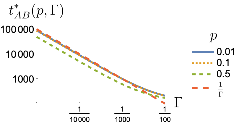
Figure 9: The crossover time $t^{*}_{AB}$ at various probability of measurement $\Gamma$, which is independent of the system size. The size used to produce the plot is $N=250$, As $N$ increases, the curve starts to flatten and deviate at large $\Gamma$. The dashed red line ($1/\Gamma$) is a guide to the eye.

To summarize the dynamical regimes of finite-size random circuits with or without measurement or dissipation, a key ingredient is the restriction on domain wall growth in both the space and the time dimensions. Measurement and dissipation play very different roles when they are both present in the system; independently however, either will reduce the entanglement of the steady state. When dissipation is absent, one recovers the well-known cases of entanglement growth in (monitored) random unitary circuits, shown in FIG.10(a) and entanglement does not decay after a saturation time linear in $N$.

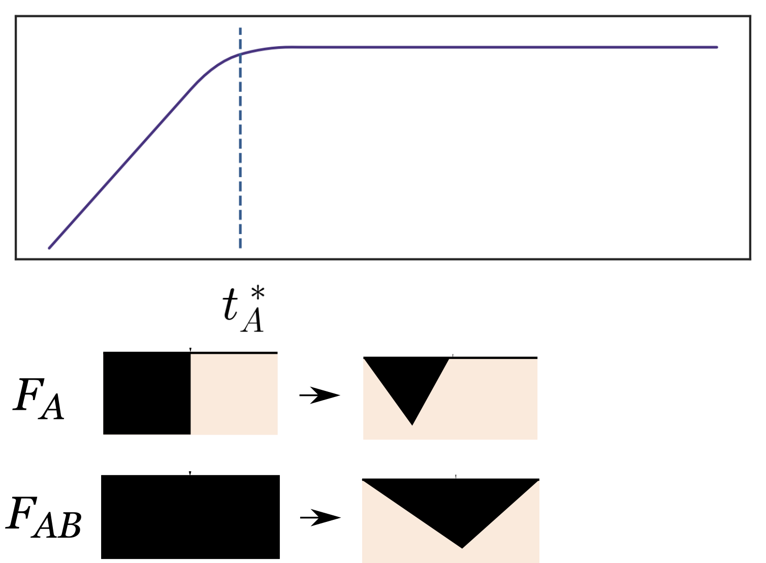
(a)

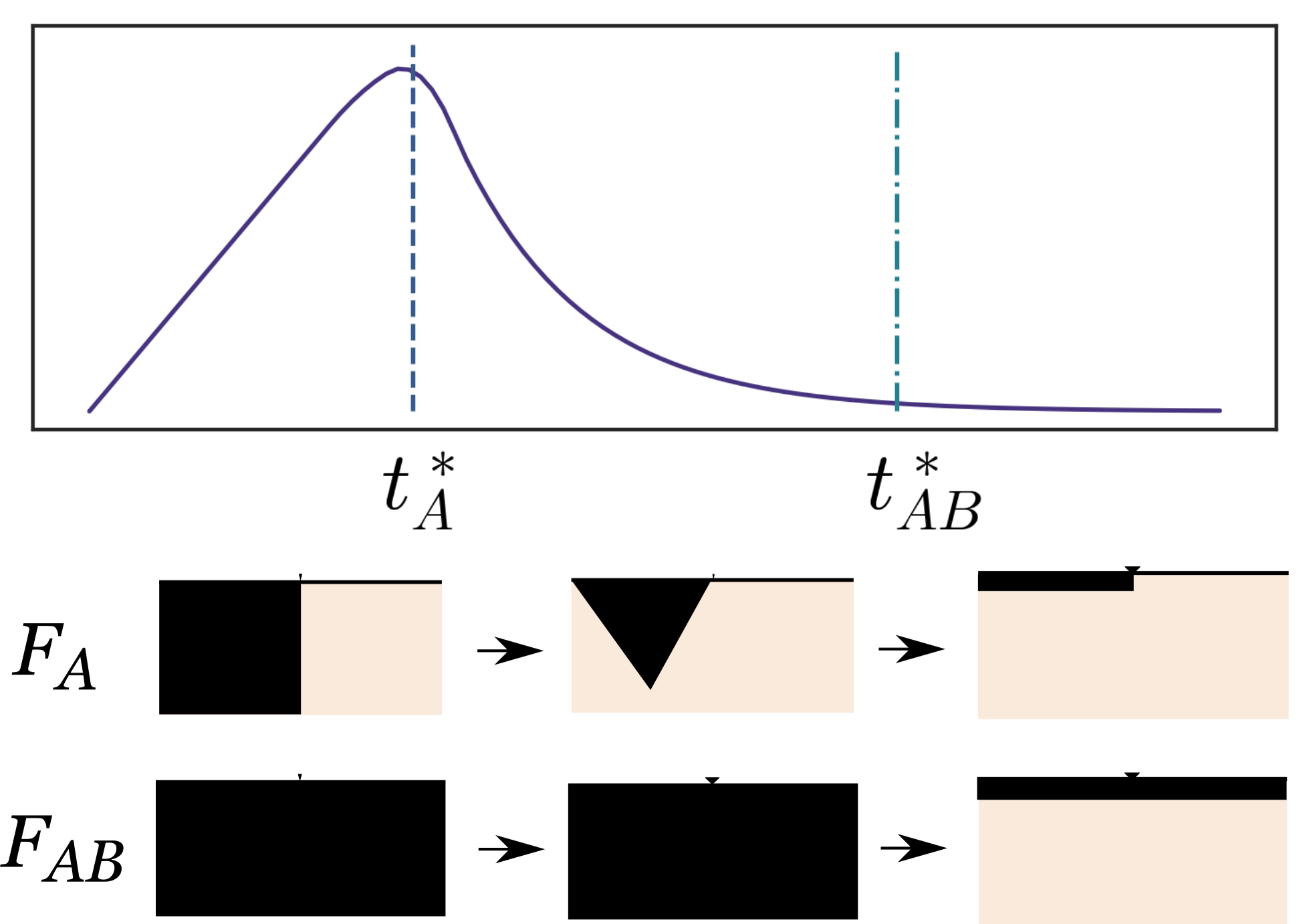
(b)

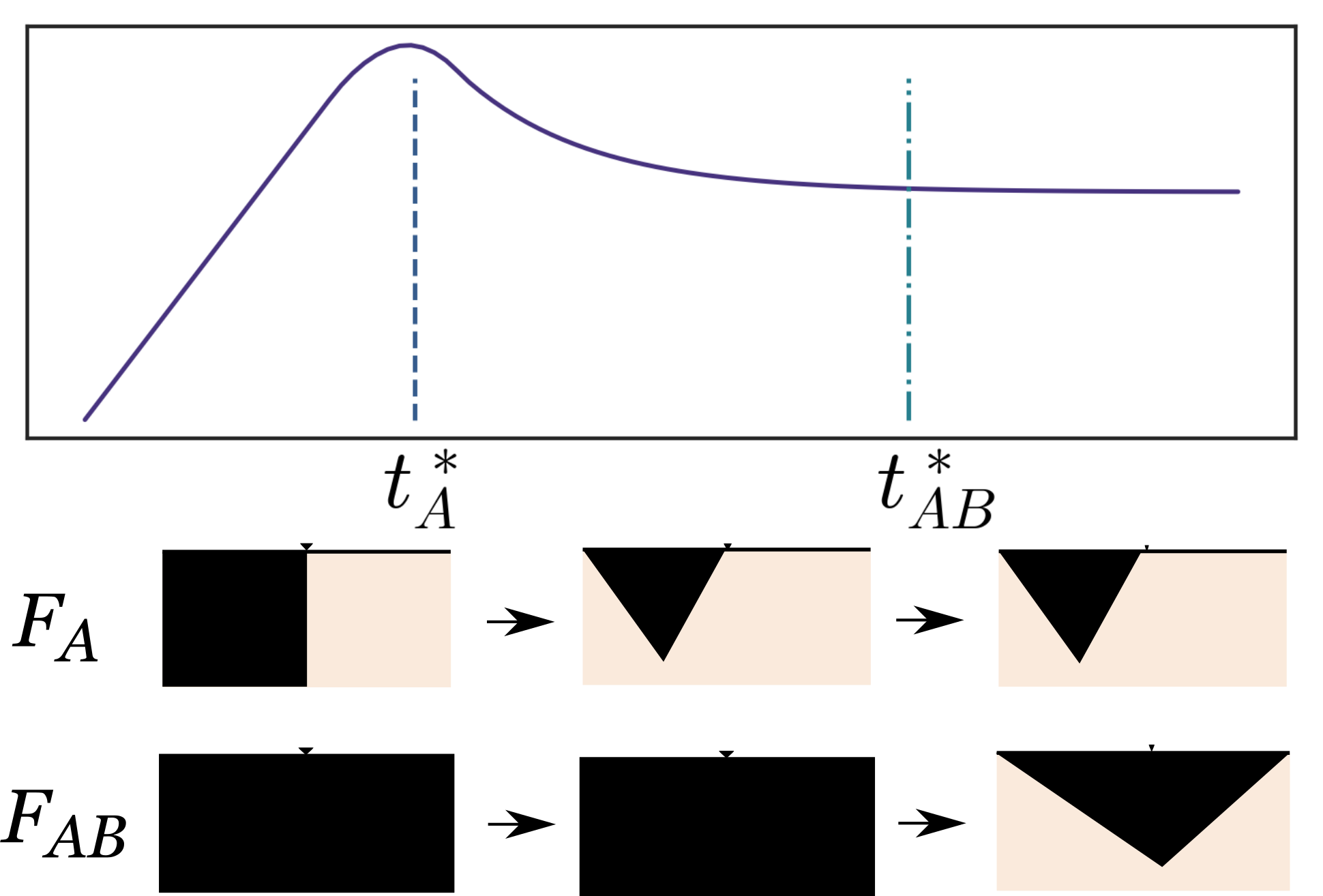
(c)

Figure 10: The dynamics of the mutual information when (a) $p\geq 0$ and $\Gamma=0$, (b) $p=0$ and $\Gamma>0$, and (c) $p>0$ and $\Gamma>0$ for finite systems.

With dissipation but without measurements, entanglement grows ballistically initially as the domain wall stretches in time, but then decays to zero because $F_{A}B$ grows longer than $F_{A}$ given that nucleating a domain wall without an appropriate boundary condition is more difficult. In the end, the classical domain wall will stick to the final time slice as it is the most energetically favorable, shown in FIG.10(b). The unitary dynamics does not create more entanglement between the disparate elements within the principal system, and the steady state becomes classical.

With both measurement and dissipation, the initial growth phase does not change. However, measurement and dissipation have competing effects in the statistical mechanical model and on the steady state. The dissipation causes the mutual information to fall off as in the previous case, but the measurement keeps the state from being completely mixed. In the classical model, the measurement leaves some room for $\downarrow$ in a finite system, but compared to the non-dissipative case, its domain wall will be closer to the top boundary due to the biased fields, so the free energy or the mutual information in the quantum model is less than that of the 10(a) and more than that of 10(b), as seen in FIG. 10(c).

III.4.5 Comments on the time scales as $N\to\infty$

For finite-size systems, we have found two timescales $t^{*}_{A}$ and $t^{*}_{AB}$, where the former depends on $N$. This cannot happen in the thermodynamic limit, because the entanglement should not grow linearly forever when it is coupled to an infinite bath. However, the difference between finite and infinite $N$ is that the parametric energy difference between the domain wall configurations (FIG.6) does not matter at finite times as long as the difference does not increase with the system size. This means that for $F_{AB}$, $\mathcal{O}(1)$ number of diagonal domain walls are allowed as long as it does not grow with the horizontal extent of the system $N$, even if the boundary condition does not induce a domain wall, and the free energy is lowered by the domain walls due to their fluctuations. The energy of the diagonal domain wall which scales with 2$t$ is infinitesimal compared to the bulk uniform which scales roughly with $tN$ and it will be compensated by nucleating a region of around $t=0$ slice that costs less than , which scales with $t^{2}$. The transition to the steady state will then be the same for $F_{A}$ and $F_{AB}$, both of which will be described by changing from a trapezoid at short times to a hanging horizontal domain wall in the long time limit,

$$F_{A}\hskip 14.22636pt\vbox{\hbox{\includegraphics[scale={0.5}]{diagrams/F_A_trapez.png}}} \Rightarrow\vbox{\hbox{\includegraphics[scale={0.5}]{diagrams/F_A_bdry_Ninfty.png}} }$$

$$F_{AB}\hskip 14.22636pt\vbox{\hbox{\includegraphics[scale={0.5}]{diagrams/F_AB_trapez.png}}} \Rightarrow\vbox{\hbox{\includegraphics[scale={0.5}]{diagrams/F_AB_bdry_Ninfty.png}} }$$

The time of transition $t^{*}$ can be obtained by setting the two free energies to be equal and in the large $N$ limit, it is the same time scale where the $F_{A}$ in (29) becomes that in (24) with finite depth and it will be $N$ independent. If we ignore the depth of the hanging horizontal domain wall, we could estimate this by

$$t^{*}=\frac{\log w(\downarrow\downarrow\uparrow)-\log w(\uparrow\uparrow\uparrow)}{\log w(\downarrow\downarrow\downarrow)-\log w(\uparrow\uparrow\uparrow)},$$ (35)

where costs $\Gamma$ more than , so this time scale again scales with $\frac{1}{\Gamma}$, as expected Li et al. (2023).

This new configuration also has an impact on the entanglement velocity calculated in III.4.2, which is now time-dependent. The extra diagonal domain walls and the larger area in $F_{AB}$ than that in $F_{A}$ will reduce the velocity in time and changes the sign of the velocity at a finite, $N$-independent cross-over time $t_{s}$. This is difficult to estimate as it depends on the number of diagonal domain walls/trapezoids, even if it is constrained to be $\mathcal{O}(1)$, and on the depth at which the trapezoids emerge. A scenario in which the sign of the velocity can change is the following

$$F_{A}\hskip 14.22636pt\vbox{\hbox{\includegraphics[scale={0.5}]{diagrams/F_A_full_v.png}}}\xRightarrow{t_{s}}\vbox{\hbox{\includegraphics[scale={0.5}]{diagrams/F_A_trapez.png}}} \xRightarrow{t^{*}}\vbox{\hbox{\includegraphics[scale={0.5}]{diagrams/F_A_bdry_Ninfty.png}} }$$

$$F_{AB}\hskip 14.22636pt\vbox{\hbox{\includegraphics[scale={0.5}]{diagrams/F_AB_full_v.png}}}\xRightarrow{t_{s}}\vbox{\hbox{\includegraphics[scale={0.5}]{diagrams/F_AB_trape_v.png}}} \xRightarrow{t^{*}}\vbox{\hbox{\includegraphics[scale={0.5}]{diagrams/F_AB_bdry_Ninfty.png}} }$$

where the top row describes the state changing in $F_{A}$ and the bottom row describes the state changing in $F_{AB}$. The left frame occurs at the extremely short time $t<t^{*}_{A}$. The middle frame describes a decrease of the mutual information as the number of domain walls in $F_{AB}$ outnumbers that in $F_{A}$ and $F_{B}$ combined. This change is accompanied by enhanced fluctuations as vertical domain walls will merge areas of the same spin in the vicinity of each other. Nevertheless, this argument about the relation between the two timescales $t_{s}<t^{*}$ provides an intuitive picture of how area law entanglement in the steady state is reconciled with ballistic short-time entanglement growth in an infinite system. The entanglement dynamics should be comparable to that in FIG. 10(c), with $t_{A}$ substituted by $t_{s}$ and $t_{AB}$ by $t^{*}$.

While the above rough estimations of crossover times for small systems largely ignored entropic contributions, these are needed for computing precise values of the mutual information in the steady state. Prior work on monitored unitary circuits has mapped the resulting fluctuating domain walls onto a directed polymer problem, with projective measurements acting like random attractive potentials $V(x,t)$ in the bulk Li et al. (2021); Li and Fisher (2021). The kinetic energy of these polymers comes from the thermal fluctuation that we have ignored. The boundary condition plays a vital role in computing mutual information. If the mixed boundary condition does not change the bulk state of the lattice magnets, e.g. the completely polarized state, or the nature of the polymers, the mutual information $\tilde{I}^{(2)}_{A:B}$ will only keep an $\mathcal{O}(1)$ area law contribution. In the statistical mechanical description, this means that the polymers in $F_{A}$ and $F_{B}$ would be treated as two halves of the polymer in $F_{AB}$, and $F_{A}+F_{B}-F_{AB}-F_{\emptyset}=-\tilde{I}_{A:B}\leq 0$, since entropy increases when a substance is divided into multiple parts. This is not the correct assumption, because the polymer in $F_{AB}$ is a closed contour in the bulk, and cutting it will result in two free floating polymers with much larger entropy than the polymers pinned at the two ends in $F_{A}$ and $F_{B}$. If the energy still roughly cancels up to $\mathcal{O}(\log N)$ between the classical models with different boundary conditions, we quote the free energy difference between the two types of polymer in capillary wave theory that is $\frac{5}{2}\log N$ Li and Fisher (2021) in the case where measurement is absent. However, the final mutual information does depend on $p$ and $\Gamma$ in Weinstein et al. (2022) and our section IV which will require revisions to explain the steady state entanglement in a monitored dissipative system. We note that in our case, dissipation acts like a long-range gravitational attraction to the top boundary that wants to minimize the area of $\downarrow$ enclosed. This long-range potential controlled by $\Gamma$ will compete with the other localized potential $V(x,t)$ controlled by $p$ in determining the surface tension, and hence the saddle points. A refinement of the classical theory is therefore required to have analytic control over the steady state mutual information.

IV Numerical simulations

To check the qualitative dynamical trends as a function of $p$ and $\Gamma$ for the quantum system, we now simulate the monitored random-unitary + amplitude damping circuit for small qubit chains up to $N=14$ following FIG.1(a) using exact many-body density matrix trajectories. At every layer, we first apply the Haar random unitary matrix to the two nearest neighboring qubits, then evolve individual qubits by the Kraus operators for the dissipative channel. Subsequently, each qubit is subjected to a projective measurement at random times, governed by the probability $p$. The circuit can be considered as a Trotter decomposition of a monitored qubit chain that slowly dissipates into a Markovian environment. To improve the numerical efficiency of the density matrix evolution, we optimize tensor contraction between gates and qubits which halves the run time compared to brute force matrix multiplication for the open N-body quantum systems. The dimensionless quantity $\Gamma$, the probability of making measurements $p$ and the system size $N$ determine dynamics and steady-state entanglement, which we study by computing the von Neumann mutual information

$$I_{A:B}(\rho) =S(\rho_{A})+S(\rho_{B})-S(\rho)$$ (36)

via simulating the per-measurement-sequence density matrix trajectories and averaging over measurements. $\{A,B\}$ is an equal size partition of the system with periodic boundary condition. Complementary behavior for the logarithmic negativity is shown in Appendix.C. Results are presented in the parameter space $(p,\Gamma)$ where $p\in[0,0.6]$ and $\Gamma\in[10^{-4},10^{-2}]$. The range of probabilities encompasses the critical $p_{c}$ that have been observed and predicted for pure-state trajectories with monitored measurements Nahum et al. (2013); Zabalo et al. (2020); Bao et al. (2020). We focus on weak but non-negligible dissipation rates; for instance, $\Gamma=10^{-3}$ has been used to test error propagation in Noisy Intermediate Scale Quantum (NISQ) devices González-García et al. (2022). While simulable system sizes $N$ remain too small to resolve critical points and scaling exponents for pure-state dynamics, the central object of interest in our work is the competition between dissipation and monitored measurements in governing the short-time entanglement dynamics, to identify peak regimes of mutual information growth, useful for optimizing entanglement generation in quantum systems in a noisy environment. The behavior of the dephasing channel is similar to the amplitude damping channel at small $\Gamma$, which we will not analyze in this work. The difference kicks in only at large $\Gamma$ when the qubit chain completely thermalizes with the environment.

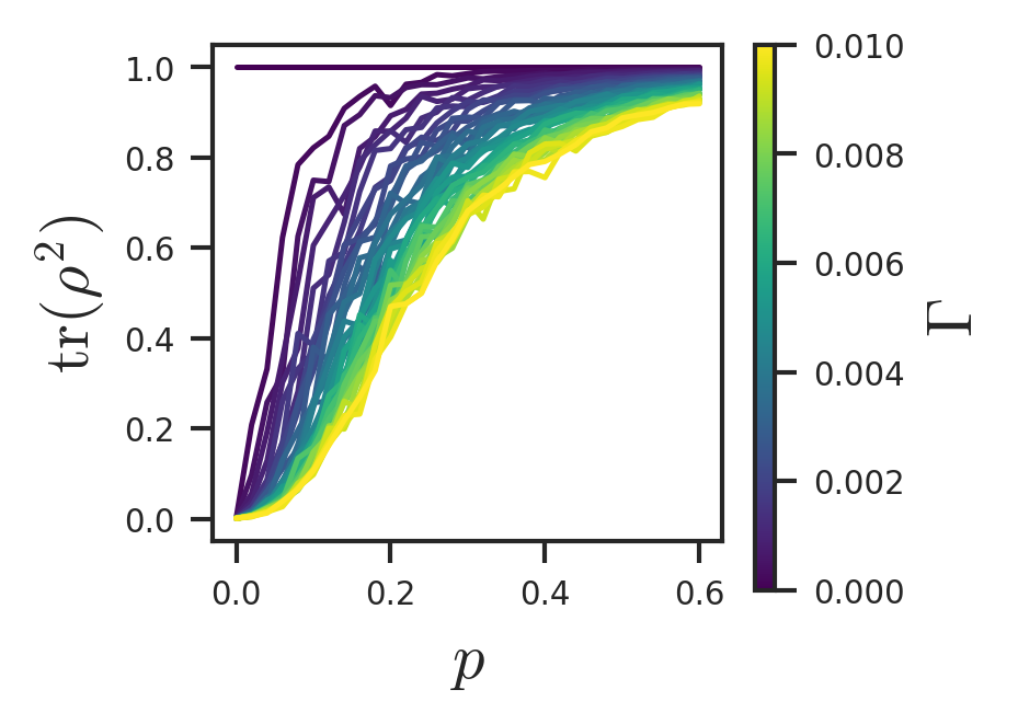
Figure 11: The dependence of the purity of the total steady state on the probability of measurement for different $\Gamma$.

We choose an initial pure product state, which generically evolves into a mixed state as a function of $\Gamma$ while simultaneously subjected to measurement purification 11. For large $\Gamma\gg 1$, the state will evolve into the unique ground state of the Lindblad operator. A higher rate of dissipation renders lower purity at a given probability of measurement, as long as $\Gamma<1$, while measurements purify the states (FIG.11). Another limit where the steady state is pure is when the dissipation rate is large enough, e.g. $\Gamma>1$, the state will evolve into the unique ground state of $\sigma_{-}^{\otimes N}$.

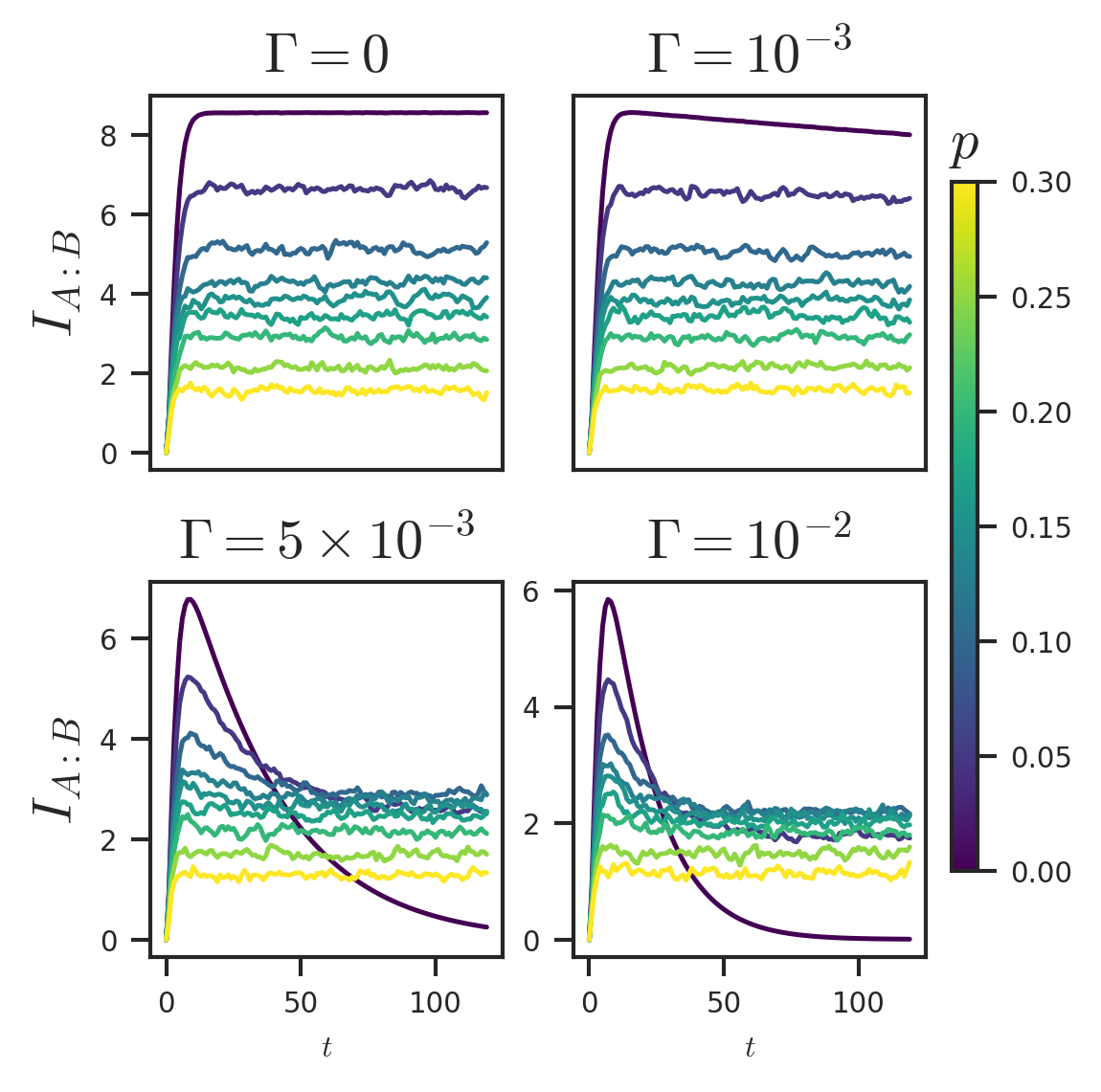
(a)

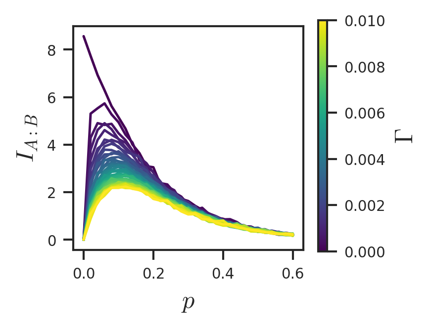
(b)

Figure 12: (a) The dynamics of the mutual information within the same time frame at 3 decades of dissipation rates $\Gamma$. The colorbar marks the probability of measurement $p$. The system size is $N=10$ qubits. Each point in time is averaged over 200 independent trajectories over random Haar measure, projective measurements randomly located in space-time, and the random measurement outcomes. (b) The mutual information of the steady state as a function of the probability of measurement with at different values of dissipation rates. The colorbar marks the dissipation rate $\Gamma$.

The dynamics of the von Neumann mutual information and the negativity agree qualitatively with the picture presented in section III.4 from the perspective of the effective classical theory for small systems $N$. At very short times, the entanglement grows ballistically. We fit a linear function to the growth within time $N/2$ (FIG.12(a)), estimated by $t_{A}^{*}$. The resulting entanglement velocity $v_{1}$ decreases with increasing $p$ and $\Gamma$, shown in FIG.13, similar to $v_{2}$ predicted in FIG.7. The increase in the mutual information terminates smoothly around a time proportional to $t^{*}_{A}$ that is shortened by both measurement and dissipation, seen directly from the dynamics (FIG.12(a)). Note that the numerical saturation time $t_{\mathrm{sat}}$, estimated in Appendix C, upper bounds $t_{A}^{*}$ in section III.4.3 for fixed $(p,\Gamma)$.

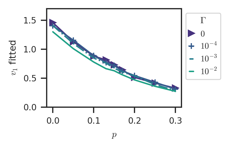
Figure 13: The fitted velocity of increase in the mutual information at short times in system size $N=10$.

At longer times, the dissipative evolution shows an exponential decay, the time scale of which is controlled by $1/\Gamma$. Larger probability of measurement prevents the steady state from becoming completely mixed while shortening the waiting time. This $1/\Gamma$ waiting time behavior in the Lindblad system again agrees qualitatively with the estimate for the crossover time $t^{*}_{AB}$ for the second Rényi entropy deduced from the classical model, which was shown to be proportional to $1/\Gamma$ and decreases with increasing $p$. This decay describes the thermalization process of the total state $\rho_{AB}$ with the environment after $t_{\mathrm{sat}}$, when most of the entanglement between $A$ and $B$ is formed.

Finally, in the steady state, the mutual information displays a non-monotonic dependence on the probability of measurement $p$ (FIG. 12(b)), which decreases the entanglement between $A$ and $B$ however, purifies the final state defined on $AB$. Unlike measurement, dissipation is only destructive in forming long-range correlations between $A$ and $B$ and drives the system towards a mixed state because individual qubits entangle with the environment as opposed to other qubits. The unitary still scrambles the information very quickly within the mixed state but cannot purify the state or retain the quantum correlation from the interaction with the environment. As a result, the mutual information at fixed $p$ monotonically decreases in $\Gamma$. The qualitative dependence of the entanglement as a function of $p$ and $\Gamma$ are consistent with previous findings Weinstein et al. (2022), which includes the peak around $p=0.1$ with varying system size. For the purpose of quantum computing, the relevant time regime with useful entanglement is therefore bounded by $t^{*}_{A}$. The estimate of $t^{*}_{A}$ for small accessible system sizes is, therefore, the main quantity of interest of this paper.

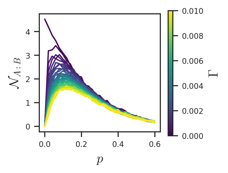
(a)

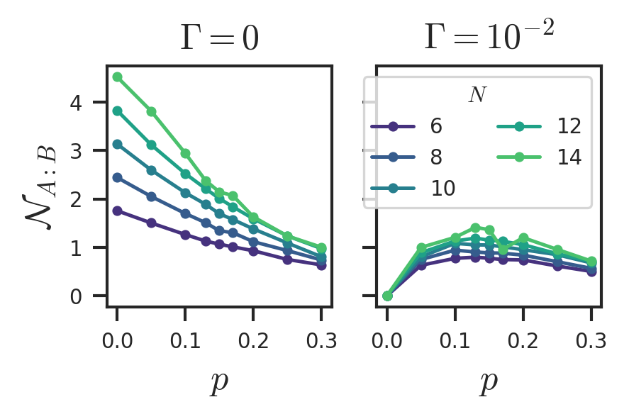
(b)

Figure 15: The dependence of the logarithmic negativity of the subsystem of half the size on the probability of making measurement $p$, where the different colors mark (a) the dissipation rate $\Gamma$ and (b) the different system sizes. In (b), the system size used in the left panel is $N=10$.

Without dissipation, measurement only serves to destroy entanglement, evident from the mutual information curves that descend with increasing probabilities of measurement in the left panel of Fig. 14 and the monotonic decreasing negativity in Fig. 15. However, with dissipation, the steady state lacks any entanglement when no measurement is made, with vanishing mutual information at $p=0$ for all dissipation rates $\Gamma$. As the probability $p$ increases, some coherence of the quantum state is recovered and peaks emerge at the sweet spots where the mutual information is maximized. This entanglement maximizing measurement rate grows slightly with increasing $\Gamma$, and the value of the peak decreases when $\Gamma$ is increased. In the left panel of FIG.14, the dissipationless qubit system is in the volume law phase when $p<p_{c}\approx 0.16$ and area law when $p>p_{c}$. In the presence of dissipation, the mutual information obeys an area law in the steady state and stops growing with the system size at large times (FIG.14, right panel). There is no transition in the probability of measurement in the case of random unitary circuits since though the classical analysis where the probability of measurement weakens the symmetry-breaking interactions, but is unable to completely recover the symmetry of the system before the domain walls become deconfined. To the extent that we understand the classical model, there is no symmetry to produce a sharp phase transition.

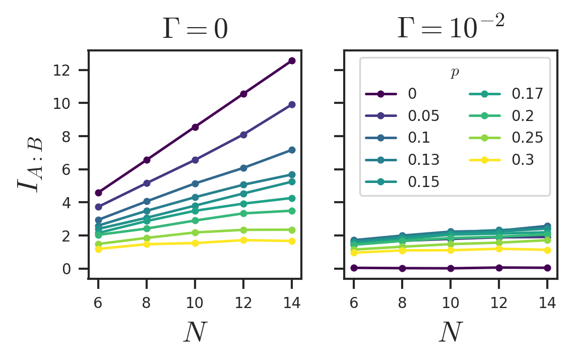
Figure 14: The scaling of the mutual information with the system size when $\Gamma=0$ and when $\Gamma=0.01$.

V Conclusion and discussions

In conclusion, we extend the mapping between random unitary circuits and classical spin models to include both dissipation and measurements. In this mapping, dissipation turns on a bias field and 3-body interactions on downward-pointing triangles in the effective Ising model, and the mutual information can be computed from free energy differences between different boundary conditions. We focus on small and accessible qubit system sizes and qualitatively estimate the short-time, intermediate time and steady-state limits of the entanglement behavior via calculating a generalized second Rényi mutual information. While the measurement-induced phase transition is absent at any finite dissipation strength, the Ising effective classical statistical model for two replica is sufficient to qualitatively understand distinct entanglement dynamical regimes. These emerge from distinct domain wall configurations as finite times of the effective Ising model. In classical theory, measurements act to push the model towards a restored Ising symmetry that was broken by dissipation, encouraging the growth of diagonal (vertical) domain walls. Conversely, dissipation serves to push the domain wall towards the pinned boundary, to minimize the area of the spins that anti-align with the biasing terms. The crossover times in the quantum entanglement can be estimated by the change in the saddle point of the classical model as time direction is stretched longer. For finite systems $N$ at low dissipation rate $\Gamma$, the entanglement first grows linearly for a time proportional to $N$ with a $\Gamma$ and measurement probability $p$ dependent velocity, then decays for a time inversely proportional to the dissipation rate $\Gamma$ to reach a steady state with area-law entanglement. We finally simulate the open system using exact diagonalization for small system sizes and confirm the qualitative behavior of time scales and entanglement speed that was estimated in the classical theory. We find in agreement with predictions that the short-time dynamics in small systems can create extensive entanglement, which can be usefully targeted for quantum computation, with a bound on achievable time scales estimated from the effective classical model.

An obvious way to improve the presented mapping is to compute quantitative measures of entanglement for mixed states such as negativity and Petz Rényi mutual information Kudler-Flam (2023); Scalet et al. (2021), which satisfies subadditivity and only depends on a single classical state instead of several with different boundary conditions. This requires a general $n$-replicated quantum system to a classical model for arbitrary $n$ and is difficult in the current scheme as the number of spin states increase with the number of replicas, but can in principle, be carried out via a diagrammatic expansion. Another approach is to extend previous analyses using directed polymers by adding long-range potentials that mimic the effect of dissipation. Improved simulations of the open quantum using tensor networkWeimer et al. (2021) or stabilizer formalism Li et al. (2023); Weinstein et al. (2022) will also permit more refined computations of time scales and transitions.

On a different front, although the tensor network models in holography are still limited in applications so far, the calculation of entanglement entropy is much more tractable in this setup, and it has been fruitful to refine the structure of bulk spatial slices by the entanglement properties of boundary subsystems. The effect of measurement on the boundary BCFT has recently been recognized as information teleportation in the bulk in the context of MPT Antonini et al. (2022); Milekhin and Popov (2022). Additionally, the recent progress in addressing the black hole information paradox relies on coupling the boundary CFT to a bath in addition to the proposal that AdS/CFT correspondence itself can be understood as quantum error correction has brought brand new insight in to the notion of bulk-boundary mapping Almheiri et al. (2015); Pastawski et al. (2015). Our classical analytic picture of the dissipative circuit is the first step towards understanding the bulk theory that is dual to a CFT coupled to a bath.

Appendix A Kraus operators for generalized dephasing channel

The dephasing channel can be written as

$$\Phi(\rho)=(1-p)\rho+p\sum_{k=0}^{d-1}\text{tr}(E_{k,k}\rho)E_{k,k}$$

where $E_{i,j}=\outerproduct{i}{j}$ is the matrix unit, $\outerproduct{i}{j}$ is in the computational basis and $d=2^{N}$ is the dimension of the Hilbert space. Its Kraus operators are the eigenvectors of the Choi operator, which can be written as $C_{\Phi}=\sum_{i,j,i\neq j}\outerproduct{ii}{jj}(1-p)+\sum_{i}\outerproduct{ii}{ii}p$. As the column space of the Choi operator is clearly spanned by states of the form $\ket{ii}$, we shorten the repeated index $\ket{ii}\to\ket{i}$. The Kraus operators will be the solution to the equation:

$$(C_{\Phi}(\rho)-\lambda\mathbb{I})\ket{\alpha} =0$$ (37)

$$\Rightarrow(1-p)\sum_{j}\langle j|\alpha\rangle\sum_{i}\ket{i}+(p-\lambda)\ket{\alpha} =0.$$

The vector equation will be 0 under two circumstances: one is when the vectors $\ket{\alpha}\propto\sum_{i}\ket{i}$, which is an eigenvector with the eigenvalue $d(1-p)+p$. The other one is when the coefficients of all the vectors are zero, i.e. $\lambda=p$ and $(1-p)\sum_{j}\innerproduct{j}{\alpha}=0$ for any $p$. Since $\ket{j}$ is summed over an orthonormal basis of the Hilbert space, to make $\sum_{j}\innerproduct{j}{\alpha}=0$, $\ket{\alpha}$ needs to be a sum of vectors with coefficients of equal magnitude and opposite signs. Since there can only be $d-1$ linearly independent eigenvectors in this subspace, without loss of generality, we write this set of eigenvectors with eigenvalue $p$ as $\{\ket{j}-\ket{0}\}_{j=1}^{d-1}$, to which we must perform the standard Gram-Schmidt orthonormalization procedure.

We use the following strong induction to show that orthonormalizing $\left\{\ket{\tilde{\lambda}_{j}}=\ket{j}-\ket{0}\right\}_{j=1}^{d-1}$ gives the generalized diagonal Gell-Mann matrices of $SU(d)$Stover ,

$$\lambda_{l}=\sqrt{\frac{2}{l(l+1)}}\left(\sum_{j=1}^{l}E_{j,j}-lE_{l+1,l+1}\right),$$

which, in our index convention, are

$$\ket{\lambda_{l}}=\sqrt{\frac{1}{l(l+1)}}\left(\sum_{j=0}^{l-1}\ket{j}-l\ket{l}\right).$$

Proof: The base case is $\ket{\lambda_{1}}=\frac{1}{\sqrt{2}}(\ket{0}-\ket{1})$, which satisfies the form. Now assume that the form holds $\forall l\leq l^{\prime}$. Then the $l=(l^{\prime}+1)$st orthonormal basis vector is:

$$\hskip 14.22636pt\ket{\accentset{\approx}{\lambda}_{l+1}}=\ket{\tilde{\lambda}_{l+1}}-\sum_{k=1}^{l}\innerproduct{\tilde{\lambda}_{k}}{\tilde{\lambda}_{l+1}}\ket{\tilde{\lambda}_{k}}$$

$$=\frac{1}{\sqrt{2}}(\ket{l+1}-\ket{0})$$

$$\hskip 28.45274pt+\frac{1}{\sqrt{2}}\sum_{k=1}^{l}\frac{1}{k(k+1)}\left(\sum_{i=0}^{k-1}\ket{i}-k\ket{k}\right)$$

$$=\frac{1}{\sqrt{2}}(\ket{l+1}-\ket{0})$$

$$\hskip 14.22636pt+\frac{1}{\sqrt{2}}\left(\sum_{i=0}^{l-1}\ket{i}\sum_{k=i+1}^{l}\frac{1}{k(k+1)}-\sum_{k=1}^{l-1}\frac{1}{k+1}\ket{k}\right)$$

$$=\frac{1}{\sqrt{2}}(\ket{l+1}-\ket{0})$$

$$\hskip 14.22636pt+\frac{1}{\sqrt{2}}\sum_{i=0}^{l-1}\left(\frac{1}{i+1}-\frac{1}{l+1}\right)\ket{i}-\sum_{i=1}^{l-1}\frac{1}{i+1}\ket{i}$$

$$=\frac{1}{\sqrt{2}}(\ket{l+1}-\ket{0})+\frac{1}{\sqrt{2}}\left(\ket{0}-\frac{1}{l+1}\sum_{i=0}^{l}\ket{i}\right)$$

$$=\frac{1}{\sqrt{2}}\left(\ket{l+1}-\frac{1}{l+1}\sum_{i=0}^{l}\ket{i}\right).$$

Normalizing this by $\sqrt{\innerproduct{\accentset{\approx}{\lambda}_{l+1}}{\accentset{\approx}{\lambda}_{l+1}}}=\sqrt{\frac{l+2}{l+1}}$ gives

$$\ket{\lambda_{l+1}}=\sqrt{\frac{1}{(l+1)(l+2)}}\left((l+1)\ket{l+1}-\sum_{i=0}^{l}\ket{i}\right).$$

q.e.d.

Combining this with the other eigenvector with the eigenvalue $d(1-p)+p$, we obtain the expressions of the Kraus operators in section II.

Appendix B Boltzmann weights in the $q\to\infty$ limit

Due to the lack of spin symmetry from dissipation, the number of distinct Boltzmann weights $w_{3}(\sigma_{1},\sigma_{2};\sigma_{3})$ proliferates rapidly as $n$ is increased. To simplify the analysis, we take the limit of a large local Hilbert space dimension $q\to\infty$, which has previously been used to make the analytical continuation $n\to 1$ tractable Zhou and Nahum (2019); Jian et al. (2020); Li et al. (2023) and recovers the Potts model limit. The Weingarten function has $1/q^{2}$ suppression in the case when the $\sigma_{3}$ and $\tau$ on the vertical bonds disagree, so we only keep the contribution from $\tau=\sigma_{3}$ when computing the three-body Boltzmann weight. Expanding $w_{3}(\sigma_{1},\sigma_{2},\sigma_{3})$ in the leading orders of $1/q^{2}$, $p$, and $\Gamma$ and assuming $1>p\gg\Gamma\gg 1/q^{2}>0$, one obtains

$$w_{3}^{(2)}(\sigma_{1},\sigma_{2};\sigma_{3})=\sum_{\tau\in\{\uparrow\downarrow\}}w_{g}(\sigma_{3},\tau)w_{d}(\sigma_{1},\tau)w_{d}(\sigma_{2},\tau)$$

$$=\sum_{\tau\in\{\uparrow\downarrow\}}\left(\frac{1}{(q^{4}-1)}\delta_{\sigma_{3}\tau}-\frac{1}{q^{2}(q^{4}-1)}(1-\delta_{\sigma_{3}\tau})\right)$$

$$\times\left(q^{2}(1-p)^{2}\delta_{\sigma_{1}\tau}\delta_{\tau\uparrow}+q^{2}(1-2\Gamma)(1-p)^{2}\delta_{\sigma_{1}\tau}\delta_{\tau\downarrow}+q((1-p)^{2}+p^{2}(1-2\Gamma))\delta_{\sigma_{1}\uparrow}\delta_{\tau\downarrow}+q((1-p)^{2}+p^{2})\delta_{\sigma_{1}\downarrow}\delta_{\tau\uparrow}\right)$$

$$\times\left(q^{2}(1-p)^{2}\delta_{\sigma_{2}\tau}\delta_{\tau\uparrow}+q^{2}(1-2\Gamma)(1-p)^{2}\delta_{\sigma_{2}\tau}\delta_{\tau\downarrow}+q((1-p)^{2}+p^{2}(1-2\Gamma))\delta_{\sigma_{2}\uparrow}\delta_{\tau\downarrow}+q((1-p)^{2}+p^{2})\delta_{\sigma_{2}\downarrow}\delta_{\tau\uparrow}\right)$$

$$=\frac{q^{4}(1-p)^{4}}{q^{4}-1}\left[\delta_{\sigma_{1}\sigma_{3}}\delta_{\sigma_{2}\sigma_{3}}-4\Gamma\delta_{\sigma_{1}\sigma_{3}}\delta_{\sigma_{2}\sigma_{3}}\delta_{\sigma_{3}\downarrow}\right]+\mathcal{O}\left(\frac{1}{q}\right)$$

$$=\frac{q^{4}(1-p)^{4}}{q^{4}-1}\left[\vbox{\hbox{\includegraphics[scale={0.5}]{triangles/domWall0.png}}}-4\Gamma\vbox{\hbox{\includegraphics[scale={0.5}]{triangles/mmm.png}}}\right]+\mathcal{O}\left(\frac{1}{q}\right),$$ (38)

where the empty plaquette means that three spins on the corners are the same. Furthermore, only terms $\mathcal{O}(\Gamma)$ are kept. From the expression above, the Boltzmann weights of and are equal without the $\Gamma$ term, and the highest order replica-symmetry-breaking term makes the weight of smaller by $4\Gamma$. To see how dissipation affects the other spin configurations on a plaquette, one must go to the next order in $1/q$, where the replica symmetric (RS) part is

$$\frac{q^{3}(1-p)^{2}((1-p)^{2}+p^{2})}{q^{4}-1}(\delta_{\sigma_{1}\sigma_{3}}+\delta_{\sigma_{2}\sigma_{3}}-2\delta_{\sigma_{1}\sigma_{3}}\delta_{\sigma_{2}\sigma_{3}})$$ (39)

and the replica-symmetry-breaking (RSB) part is

$$\frac{q^{3}(1-p)^{2}}{q^{4}-1}\Bigg{[}-2p^{2}\Gamma\delta_{\sigma_{1}\sigma_{3}}\delta_{\sigma_{2}\sigma_{3}}\delta_{\sigma_{3}\downarrow}-2\Gamma\delta_{\sigma_{1}\sigma_{3}}\delta_{\sigma_{3}\downarrow}((1-p)^{2}+p^{2})(1-\delta_{\sigma_{2}\sigma_{3}})-2\Gamma p^{2}\delta_{\sigma_{2}\sigma_{3}}\delta_{\sigma_{3}\downarrow})+(\sigma_{1}\leftrightarrow\sigma_{2})\bigg{]}$$

$$=-\frac{2\Gamma q^{3}(1-p)^{2}}{q^{4}-1}\Bigg{[}((1-p)^{2}+2p^{2})\vbox{\hbox{\includegraphics[scale={0.5}]{triangles/mmm.png}}}+((1-p)^{2}+p^{2})\vbox{\hbox{\includegraphics[scale={0.5}]{triangles/m0m.png}}}+p^{2}\vbox{\hbox{\includegraphics[scale={0.5}]{triangles/0mm.png}}}+(\sigma_{1}\leftrightarrow\sigma_{2})\Bigg{]},$$ (40)

where vertices drawn without a spin mean that the spin can point in either up or down, and repeated empty vertices in the plaquette mean that they all take the same spin but can point in either direction. We organize the Boltzmann weights of the other configurations in leading order $\frac{1}{q}$ in table 1.

domain wall configuration
spin diagram
$w_{3}^{(2)}$	$\frac{q^{4}(1-p)^{4}}{q^{4}-1}$	$\frac{q^{4}(1-p)^{4}(1-4\Gamma)}{q^{4}-1}$	$\frac{q^{2}((1-p)^{2}+p^{2}(1-2\Gamma))^{2}}{q^{4}-1}$	$\frac{q^{2}((1-p)^{2}+p^{2})^{2}}{q^{4}-1}$

domain wall configuration	or
spin diagram
$w_{3}^{(2)}$	$\frac{q^{3}(1-p)^{2}((1-2\Gamma)((1-p)^{2}+p^{2})-2\Gamma p^{2})}{q^{4}-1}$		$\frac{q^{3}(1-p)^{2}((1-p)^{2}+p^{2})}{q^{4}-1}$

Table 1: The Boltzmann weights of domain wall and spin configuration on a plaquette at the leading order of the inverse onsite Hilbert space dimension $1/q$. In the lower table, the reflection symmetry of each triangular plaquette is preserved, but the same domain wall configuration have different weights, depending on the bottom spin orientation.

Configurations that receive RSB correction at the same order as their RS configuration are the ones with $\tau=\sigma_{3}=\downarrow$. Heuristically, this follows from dissipation turning on a magnetic field in the up-spin direction Weinstein et al. (2022); Jian et al. (2021). However, we note that the weights account for a combination of a magnetic field pointing in $\downarrow$ direction and a three-body term that favors the $\uparrow$ direction as shown in section III.3. Having no domain wall costs the least energy, which is roughly 0 for or $4\Gamma$ for . The vertical domain wall costs $\log(q)$ if the bottom spin on the plaquette is $\uparrow$, and $\log(q)+2\Gamma$ if the bottom spin is $\downarrow$. Lastly, the horizontal domain wall costs $2\log q$ and $2\log q+4\Gamma$ with the same dependence on the bottom spin. If the number of $\uparrow$ and $\downarrow$ spins are not equal, then the free energy penalty compared to the homogeneous ground state scales like $N^{2}\log(1-4\Gamma)\approx-4N^{2}\Gamma$ where $N^{2}$ is the size of the 2D lattice.

Appendix C Scaling of entanglement and negativity of the quantum circuits

As mentioned in the main text, the logarithmic negativity has similar behavior to the mutual information, and it is an actual entanglement monotone, i.e. it does not increase under completely positive trace-preserving maps Vidal and Werner (2002). It is defined as

$$\mathcal{N}_{A:B}=\log\Tr{\sqrt{||\rho^{T_{A}}||^{2}}},$$ (41)

where $T_{A}$ means the partial transpose on subsystem $A$. The logarithmic negativity is additive and computes the amount of entanglement distillable. The steady-state logarithmic negativity also forms a peak in probability of measurement $p$, and monotonically decreases as a function of $\Gamma$. An increase in $\Gamma$ from $10^{-3}$ to $10^{-2}$ halves the maximum of log negativity at the $p_{\text{max}}\approx 0.1$. At $\Gamma=10^{-2}$, the negativity and the mutual information cannot scale linearly with $N$ at any $p$ and the system is deep in the area law phase.

Due to the noise in the dynamics and finite system size, we hand pick $t_{\mathrm{sat}}$ where the mutual information saturates or peaks. The transition time is picked such that before $t_{\mathrm{sat}}$, the mutual information monotonically increases in time, and after $t_{\mathrm{sat}}$ the only tolerable increases in mutual information is due to fluctuation. The saturation time has the same trend as $t^{*}_{A}$ in section III.4.3, which decreases with $p$ and $\Gamma$. Due to the small system size, the saturation time is too close to differentiate the $\Gamma=0$ and $10^{-4}$ cases, and as $\Gamma$ increases, the curves of $t_{\mathrm{sat}}$ develop a meaningful difference. We expect that the saturation time will smoothly decay to 0 as a function of $p$ and $\Gamma$.

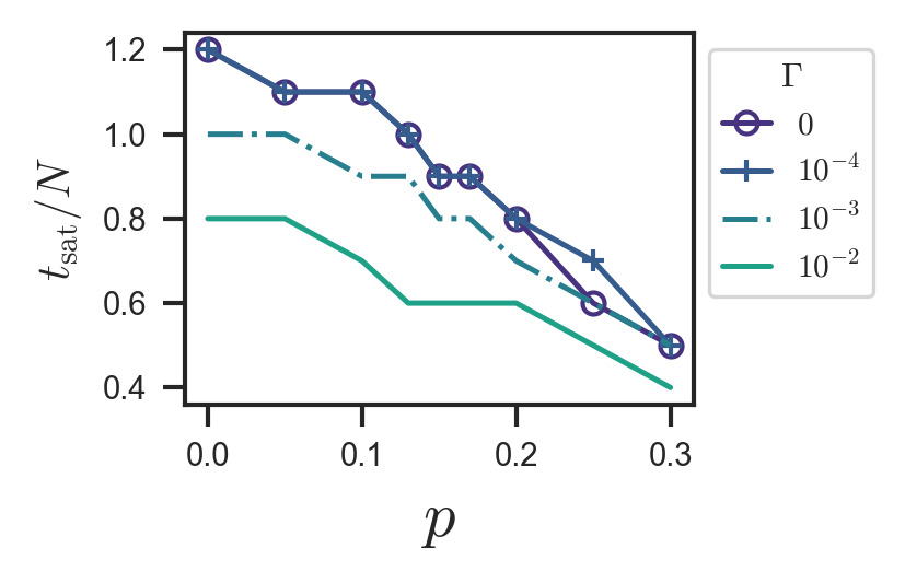
Figure 16: The estimated peak time divided by the system size. The system size giving this plot is $N=10$, so there is not enough time to resolve the saturation time at $\Gamma=0$ and $\Gamma=10^{-4}$.

References

- Hayden et al. (2016) Patrick Hayden, Sepehr Nezami, Xiao-Liang Qi, Nathaniel Thomas, Michael Walter, and Zhao Yang, “Holographic duality from random tensor networks,” Journal of High Energy Physics 2016 (2016).
- Swingle (2012) Brian Swingle, “Entanglement renormalization and holography,” Phys. Rev. D 86, 065007 (2012).
- Pastawski et al. (2015) Fernando Pastawski, Beni Yoshida, Daniel Harlow, and John Preskill, “Holographic quantum error-correcting codes: toy models for the bulk/boundary correspondence,” Journal of High Energy Physics 2015 (2015), 10.1007/JHEP06(2015)149.
- Dong et al. (2016) Xi Dong, Daniel Harlow, and Aron C. Wall, “Reconstruction of bulk operators within the entanglement wedge in gauge-gravity duality,” Phys. Rev. Lett. 117, 021601 (2016).
- Peres (1985) Asher Peres, “Reversible logic and quantum computers,” Phys. Rev. A 32, 3266–3276 (1985).
- Knill (2005) E. Knill, “Quantum computing with realistically noisy devices,” Nature 434, 39–44 (2005).
- Lassen et al. (2010) Mikael Lassen, Metin Sabuncu, Alexander Huck, Julien Niset, Gerd Leuchs, Nicolas J. Cerf, and Ulrik L. Andersen, “Quantum optical coherence can survive photon losses using a continuous-variable quantum erasure-correcting code,” Nature Photonics 4, 700–705 (2010).
- Aolita et al. (2015) Leandro Aolita, Fernando de Melo, and Luiz Davidovich, “Open-system dynamics of entanglement: a key issues review,” Reports on Progress in Physics 78, 042001 (2015).
- Casini et al. (2014) Horacio Casini, Marina Huerta, and José Alejandro Rosabal, “Remarks on entanglement entropy for gauge fields,” Phys. Rev. D 89, 085012 (2014).
- Ryu and Takayanagi (2006) Shinsei Ryu and Tadashi Takayanagi, “Holographic derivation of entanglement entropy from the anti–de sitter space/conformal field theory correspondence,” Phys. Rev. Lett. 96, 181602 (2006).
- Hubeny et al. (2007) Veronika E. Hubeny, Mukund Rangamani, and Tadashi Takayanagi, “A covariant holographic entanglement entropy proposal,” Journal of High Energy Physics 2007, 062 (2007).
- Faulkner et al. (2013) Thomas Faulkner, Aitor Lewkowycz, and Juan Maldacena, “Quantum corrections to holographic entanglement entropy,” Journal of High Energy Physics 2013 (2013), 10.1007/JHEP11(2013)074.
- Li et al. (2019) Yaodong Li, Xiao Chen, and Matthew P. A. Fisher, “Measurement-driven entanglement transition in hybrid quantum circuits,” Phys. Rev. B 100, 134306 (2019).
- Li and Fisher (2021) Yaodong Li and Matthew P. A. Fisher, “Statistical mechanics of quantum error correcting codes,” Phys. Rev. B 103, 104306 (2021).
- Nahum et al. (2018) Adam Nahum, Sagar Vijay, and Jeongwan Haah, “Operator spreading in random unitary circuits,” Phys. Rev. X 8, 021014 (2018).
- Nahum et al. (2017) Adam Nahum, Jonathan Ruhman, Sagar Vijay, and Jeongwan Haah, “Quantum entanglement growth under random unitary dynamics,” Phys. Rev. X 7, 031016 (2017).
- Zhou and Nahum (2019) Tianci Zhou and Adam Nahum, “Emergent statistical mechanics of entanglement in random unitary circuits,” Phys. Rev. B 99, 174205 (2019).
- Jonay et al. (2018) Cheryne Jonay, David A. Huse, and Adam Nahum, “Coarse-grained dynamics of operator and state entanglement,” (2018).
- Lubensky (1983) Tom C. Lubensky, “Thermal and geometrical critical phenomena in random systems,” in Ill-Condensed Matter (North-Holland Publishing Company and World Scientific Publishing Co., 1983) pp. 405–475.
- Jian et al. (2020) Chao-Ming Jian, Yi-Zhuang You, Romain Vasseur, and Andreas W. W. Ludwig, “Measurement-induced criticality in random quantum circuits,” Phys. Rev. B 101, 104302 (2020).
- Botzung et al. (2021) T. Botzung, S. Diehl, and M. Müller, “Engineered dissipation induced entanglement transition in quantum spin chains: From logarithmic growth to area law,” Phys. Rev. B 104, 184422 (2021).
- Bao et al. (2020) Yimu Bao, Soonwon Choi, and Ehud Altman, “Theory of the phase transition in random unitary circuits with measurements,” Phys. Rev. B 101, 104301 (2020).
- Weinstein et al. (2022) Zack Weinstein, Yimu Bao, and Ehud Altman, “Measurement-induced power-law negativity in an open monitored quantum circuit,” Phys. Rev. Lett. 129, 080501 (2022).
- Li et al. (2023) Zhi Li, Shengqi Sang, and Timothy H. Hsieh, “Entanglement dynamics of noisy random circuits,” Phys. Rev. B 107, 014307 (2023).
- Jian et al. (2021) Shao-Kai Jian, Chunxiao Liu, Xiao Chen, Brian Swingle, and Pengfei Zhang, “Measurement-induced phase transition in the monitored sachdev-ye-kitaev model,” Phys. Rev. Lett. 127, 140601 (2021).
- Liu et al. (2022) Shuo Liu, Ming-Rui Li, Shi-Xin Zhang, Shao-Kai Jian, and Hong Yao, “Universal kpz scaling in noisy hybrid quantum circuits,” (2022).
- Breuer and Petruccione (2007) Heinz-Peter Breuer and Francesco Petruccione, The Theory of Open Quantum Systems (Oxford University Press, 2007).
- Milz et al. (2017) Simon Milz, Felix A. Pollock, and Kavan Modi, “An introduction to operational quantum dynamics,” Open Systems & Information Dynamics 24, 1740016 (2017), https://doi.org/10.1142/S1230161217400169 .
- Bao et al. (2021) Yimu Bao, Soonwon Choi, and Ehud Altman, “Symmetry enriched phases of quantum circuits,” Annals of Physics 435, 168618 (2021), special issue on Philip W. Anderson.
- Gurvits (2003) Leonid Gurvits, “Classical deterministic complexity of edmonds’ problem and quantum entanglement,” (2003), arXiv:quant-ph/0303055 [quant-ph] .
- Vidal and Werner (2002) G. Vidal and R. F. Werner, “Computable measure of entanglement,” Phys. Rev. A 65, 032314 (2002).
- Eggarter (1975) T. P. Eggarter, “Triangular antiferromagnetic ising model,” Phys. Rev. B 12, 1933–1937 (1975).
- Nielsen and Chuang (2010) Michael A. Nielsen and Isaac L. Chuang, Quantum Computation and Quantum Information (Cambridge University Press, 2010).
- Collins (2003) Benoît Collins, “Moments and cumulants of polynomial random variables on unitarygroups, the itzykson-zuber integral, and free probability,” International Mathematics Research Notices 2003, 953–982 (2003), https://academic.oup.com/imrn/article-pdf/2003/17/953/1881428/2003-17-953.pdf .
- Skinner et al. (2019) Brian Skinner, Jonathan Ruhman, and Adam Nahum, “Measurement-induced phase transitions in the dynamics of entanglement,” Phys. Rev. X 9, 031009 (2019).
- Scalet et al. (2021) Samuel O. Scalet, Álvaro M. Alhambra, Georgios Styliaris, and J. Ignacio Cirac, “Computable Rényi mutual information: Area laws and correlations,” Quantum 5, 541 (2021).
- Kudler-Flam (2023) Jonah Kudler-Flam, “Rényi mutual information in quantum field theory,” Phys. Rev. Lett. 130, 021603 (2023).
- Li et al. (2021) Yaodong Li, Sagar Vijay, and Matthew P. A. Fisher, “Entanglement domain walls in monitored quantum circuits and the directed polymer in a random environment,” (2021).
- Nahum et al. (2013) Adam Nahum, J. T. Chalker, P. Serna, M. Ortuño, and A. M. Somoza, “Phase transitions in three-dimensional loop models and the sigma model,” Phys. Rev. B 88, 134411 (2013).
- Zabalo et al. (2020) Aidan Zabalo, Michael J. Gullans, Justin H. Wilson, Sarang Gopalakrishnan, David A. Huse, and J. H. Pixley, “Critical properties of the measurement-induced transition in random quantum circuits,” Phys. Rev. B 101, 060301 (2020).
- González-García et al. (2022) Guillermo González-García, Rahul Trivedi, and J. Ignacio Cirac, “Error propagation in nisq devices for solving classical optimization problems,” PRX Quantum 3, 040326 (2022).
- Weimer et al. (2021) Hendrik Weimer, Augustine Kshetrimayum, and Román Orús, “Simulation methods for open quantum many-body systems,” Rev. Mod. Phys. 93, 015008 (2021).
- Antonini et al. (2022) Stefano Antonini, Gregory Bentsen, ChunJun Cao, Jonathan Harper, Shao-Kai Jian, and Brian Swingle, “Holographic measurement and bulk teleportation,” Journal of High Energy Physics 2022 (2022), 10.1007/JHEP12(2022)124.
- Milekhin and Popov (2022) Alexey Milekhin and Fedor K. Popov, “Measurement-induced phase transition in teleportation and wormholes,” (2022).
- Almheiri et al. (2015) Ahmed Almheiri, Xi Dong, and Daniel Harlow, “Bulk locality and quantum error correction in ads/cft,” Journal of High Energy Physics 2015, 163 (2015).
- (46) Christopher Stover, “Generalized gell-mann matrix,” .