Gravity waves in strong magnetic fields
Abstract
Strong magnetic fields in the cores of stars are expected to significantly modify the behavior of gravity waves: this is likely the origin of suppressed dipole modes observed in many red giants. However, a detailed understanding of how such fields alter the spectrum and spatial structure of magnetogravity waves has been elusive. For a dipole field, we analytically characterize the horizontal eigenfunctions of magnetogravity modes, assuming that the wavevector is primarily radial. For axisymmetric modes (), the magnetogravity wave eigenfunctions become Hough functions, and they have a radial turning point for sufficiently strong magnetic fields. For non-axisymmetric modes (), the interaction between the discrete mode spectrum and a continuum of Alfvén waves produces nearly discontinuous features in the fluid displacements at critical latitudes associated with a singularity in the fluid equations. We find that magnetogravity modes cannot propagate in regions with sufficiently strong magnetic fields, instead becoming evanescent. When encountering strong magnetic fields, ingoing gravity waves are likely refracted into outgoing slow magnetic waves. These outgoing waves approach infinite radial wavenumbers, which are likely to be damped efficiently. However, it may be possible for a small fraction of the wave power to escape the stellar core as pure Alfvén waves or magnetogravity waves confined to a very narrow equatorial band. The artificially sharp features in the WKB-separated solutions suggest the need for global mode solutions which include small terms neglected in our analysis.
keywords:
asteroseismology, waves, stars: interiors, stars: magnetic fields, methods: analytical, methods: numerical1 Introduction
Stellar magnetism is a highly impactful, but often neglected, property of many main sequence stars (Ferrario et al., 2009; Vidotto et al., 2014), red giants (García et al., 2014; Stello et al., 2016a, b; Fuller et al., 2015), white dwarfs (Angel, 1977; Wickramasinghe & Ferrario, 2000; Liebert et al., 2003), and neutron stars (Thompson & Duncan, 1993; Kulkarni & Thompson, 1998; Levin, 2006) alike. In stars, such magnetic fields are expected to originate from dynamo mechanisms (Baliunas et al., 1996; Spruit, 2002; Maeder & Meynet, 2005; Brun & Browning, 2017), as fossils leftover from the star’s formation (Braithwaite & Spruit, 2004; Dudorov & Khaibrakhmanov, 2015; Ferrario et al., 2015), or from stellar mergers (Ferrario et al., 2009; Tutukov & Fedorova, 2010; Wickramasinghe et al., 2014; Schneider et al., 2019). Despite the importance and ubiquity of strong stellar magnetism, our understanding of oscillations in such highly magnetized stars remains incomplete, even at the qualitative level.
Interest in the influence of magnetic fields on nonradial stellar oscillations has been reignited in the past few years by the discovery of suppressed dipole () and quadrupole () oscillation modes in a family of red giants (Mosser et al., 2012; García et al., 2014; Stello et al., 2016a, b; Mosser et al., 2017). It is largely believed that the origin of this phenomenon is magnetic in nature, with recent work suggesting that ingoing gravity waves can damp out after either being trapped inside the core (the “magnetic greenhouse effect,” Fuller et al., 2015), refracted into high-wavenumber oscillations (Lecoanet et al., 2017), or dissipated by Alfvén waves (Loi & Papaloizou, 2017). In parallel, Li et al. (2022) have made the first-ever constraints on the interior magnetic field topology—the recent development of such new powerful observational tools further demands proportionate advances in our theoretical understanding of internal magnetogravity waves.
Efforts to understand the impact of magnetic fields on stellar oscillation modes have taken many forms, but have been limited due to the difficulty of the problem. For example, early attempts to understand magnetic effects on non-radial oscillations involved introducing a magnetic field as a small perturbation (e.g., Goossens, 1972; Goossens et al., 1976; Goossens, 1976; Mathis et al., 2021). Some of these perturbative calculations have promisingly suggested that core magnetic fields may leave imprints on the mixed-mode period spacing (Prat et al., 2019, 2020; Bugnet et al., 2021; Bugnet, 2022), in addition to their impact on dipole mode visibilities. However, magnetic mode splittings are often small except for fields large enough to strongly couple with Alfvén waves, where a perturbative treatment is largely inappropriate (Cantiello et al., 2016). While other analyses have assumed a purely horizontal field (Rogers & MacGregor, 2010; Mathis & De Brye, 2011; MacGregor & Rogers, 2011; Dhouib et al., 2022), such studies are not applicable to the general case where the radial component of the field dominates the interaction with the gravity waves.
Fuller et al. (2015) used a Wentzel–Kramers–Brillouin (WKB) approximation in both components of the wavenumber to show that magnetogravity waves are forced to be evanescent when the mode frequency lies below a characteristic frequency given by
| (1) |
where , , , , and are the angular degree, radial magnetic field, Brunt–Väisälä frequency, density, and radius, respectively. This result can also be recovered exactly when considering the coupling of gravity waves to an exactly uniform radial field geometry (see Section 62). However, while setting a useful scale for strong coupling between gravity waves and the magnetic field, this analysis relies on the assumption that the radial magnetic field is uniform at a given radius (which is not physical).
Other studies have probed the behavior of magnetogravity waves under arbitrarily complicated magnetic field geometries using a flexible ray-tracing method (Loi & Papaloizou, 2018; Loi, 2020a, b). However, crucially, this method relies heavily upon the (WKB) approximation that both the radial and horizontal components of the wavenumber are large compared to the variation scales of the magnetic field and stellar structure. In reality, the horizontal wavenumber of the observable modes likely has a comparable length scale to that of the magnetic field gradient. It is clear that a fuller understanding of magnetogravity waves must account for a magnetic field which is allowed to vary with latitude and longitude, without assuming an unrealistically large horizontal wavenumber.
Some progress on this front was made by Lecoanet et al. (2017), who solve for the eigenmodes of a two-dimensional Cartesian analogue of a multipole magnetic field geometry, demonstrating that modes in their model cannot propagate in regions whose magnetic field exceeds a critical strength (see Section A.2) close to the estimate of Equation 1. However, since their analysis cannot capture modes which propagate horizontally relative to the field (i.e., non-axisymmetric modes), the possibility is left open that such non-axisymmetric modes may propagate deeper into a star. Later, Lecoanet et al. (2022) extended this analysis numerically to more general tesseral/sectoral () modes using the dedalus code in order to probe the interior field of a main sequence B-type star HD 43317. However, explanations for many qualitative properties of the solution have heretofore remained elusive.
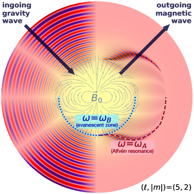
In this work, we analyze the horizontal structure of modes under a strong magnetic field. We assume that the wavevector is primarily radial, and the radial wavelengths of the perturbations are much smaller than the stellar structure length scale (the radial WKB approximation), and numerically solve for the magnetogravity mode eigenfunctions. We find that such modes contain sharp features in the fluid displacements at the locations of resonances with Alfvén waves (so-called “critical latitudes”), and that the general structure of their branches and eigenfunctions are sensitive to even vanishingly small amounts of dissipation. We also discuss the importance of the horizontal component of the field near these critical latitudes, as well as near the equator. Nevertheless, we still find that modes cannot propagate arbitrarily deep in sufficiently magnetized stars, and are likely converted into outgoing slow magnetic waves that dissipate inside of the star. An outline of the solution described in this work is shown in Figure 1.
We organize this paper as follows. In Section 2, we describe the problem setup: a stably stratified, magnetized star obeying the incompressible MHD equations (Section 2.1), whose essential physics are governed by the relationship between the mode, Alfvén, and magnetogravity frequencies , , and (Section 2.2). For the majority of this work, we specialize to a dipole magnetic field (Section 2.3). In the WKB limit, the resulting differential eigenproblem contains singularities at critical latitudes corresponding to resonances with the Alfvén spectrum. We point out a close analogy with the rotational problem (Section 3.1), then comment on previous work on internally singular eigenproblems (Section 3.2), and lastly investigate the behavior of eigenfunctions around those critical latitudes (Section 3.3). In Section 4, we present zonal (; Section 4.1) and sectoral/tesseral (; Section 4.2) solutions to the problem. We then comment on the origin and behavior of the continuous Alfvén wave spectrum (Section 4.3). However, since vanishingly small dissipation can qualitatively affect the mode spectrum, we present numerical solutions of dissipative solutions in Section 5, first allowing for evanescent solutions (Section 5.1) and then constraining the radial phase velocity (Section 5.2). Finally, in Section 6, we discuss the importance of horizontal field terms near the critical latitudes and equator (Section 6.1), nonharmonic solutions of singular differential equations (Section 6.2), the effects of more general magnetic field geometries (Section 6.3), and the possibility of magnetically stabilized modes in convective zones (Section 6.4). Section 7 concludes.
2 Problem statement
In this work, we consider a spherically symmetric star in hydrostatic equilibrium, with a possibly large equilibrium magnetic field (which is not spherically symmetric). It is assumed that the magnetic field does not act on the background structure, i.e., it is not strong enough to introduce substantial departures from a spherically symmetric stellar profile. For simplicity, we ignore rotation and use the incompressible and Cowling approximations, such that buoyancy and magnetic forces dominate the dynamics. These forces are likely to dominate in, e.g., the slowly rotating radiative cores of red giants.
Throughout this work, we use the term “magnetogravity wave” to refer to the general phenomenon of a gravity wave propagating through a highly conductive, magnetized fluid. In sufficiently magnetized stars, ingoing magnetogravity waves are refracted outwards, and (as we will show in Sections 4.1, 4.2, and 5.2) approach infinite radial wavenumber at a finite height—we refer to such waves as “slow magnetic waves.” Such branches are “slow” in the sense that their phase and group velocities approach zero as waves propagate outwards. This medium also sustains “Alfvén waves,” which are confined to magnetic field lines and appear as highly localized, linearly independent toroidal solutions to the fluid equations (see Section 4.3).
In this Section, we first introduce the linearized fluid equations (Section 2.1). We then identify the most important dimensionless parameters governing the physics (Section 2.2). Finally, we specialize to the case of a dipole magnetic field (Section 2.3), to which the majority of this work is dedicated.
2.1 Linearized fluid equations
The linearized incompressible MHD equations are
| (2a) | |||
| (2b) | |||
| (2c) | |||
| (2d) | |||
where is the perturbed fluid displacement, while , , and are the Eulerian density, pressure, and magnetic field perturbations, and subscripts indicate non-perturbed quantities (Proctor & Weiss, 1982). Here, is the Brunt–Väisälä frequency, and is the inward gravitational acceleration. Here, we have assumed the WKB approximation in the radial direction only, and have made the Cowling approximation (). Additionally, as implied by Equation 2c, we only consider adiabatic oscillations. Equation 2d is simply the induction equation in ideal magnetohydrodynamics, written in the WKB limit (for varying radially on a length scale ). Throughout this paper, we will focus on solving for oscillation modes with harmonic time dependence, i.e., those with (although this assumption is discussed in Section 6.2).
Describing an incompressible fluid under ideal magnetohydrodynamics, these equations admit modes which are restored by buoyancy and magnetism (i.e., there are no acoustic waves). Gravity waves are expected to have large radial wavenumbers which are much larger than both their horizontal wavenumbers ( in typical red giant cores) and the star’s structural variation scale . However, the horizontal wavenumber , so low- magnetogravity modes vary horizontally on similar length scales to large-scale magnetic fields. Therefore, we have adopted a WKB approximation in the radial direction only (i.e., ) such that is assumed to be larger than any structural gradients.
We define the Alfvén frequency , where is the Alfvén velocity. Then the assumption that entails that , such that the horizontal component of the magnetic field is unimportant as long as and are comparable. This approximation is made by Fuller et al. (2015), and is very analogous to the “traditional approximation of rotation” (see Section 3.1). We discuss the importance of terms in Section 6.1.
When a WKB approximation is made in both the vertical and horizontal directions (or if a monopolar field is considered; Appendix A), the dispersion relation is given by
| (3) |
where is the radial component of the Alfvén velocity (Unno et al., 1989). If both buoyancy and magnetism are important, all three terms in Equation 3 are of the same order. This defines a hierarchy of variables: letting be a small quantity around which we implicitly expand, we see that, if , then are “large” and is “small.” Hereafter, we only retain terms leading-order in , which is realistic as long as .
2.2 Important frequency scales
To understand the nature of this magnetogravity problem, we can non-dimensionalize the relevant physics equations. All formulations of the magnetogravity problem (see, e.g., Appendix A) that make similar assumptions to ours can be formulated as the following horizontal eigenproblem at a given radius (see Section 6.3):
| (4) |
where is some geometry-dependent differential operator that depends on the ratio of the Alfvén frequency to the mode frequency . In Equation 4, is a measure of the the Alfvén velocity at a given radius. Although the magnetic field strength clearly varies as a function of and , hereafter we use to denote its maximum value at a given radius.
The Buckingham theorem (Vaschy, 1892; Federman, 1911; Riabouchinsky, 1911; Buckingham, 1914) states that, for some equations depending on dimensionful quantities in independent dimensions, those equations can be written in terms of dimensionless quantities which completely determine their behavior. In this particular problem, Equation 4 depends on the dimensionful quantities , , , and , and over the independent dimensions, length and time. Therefore, the essential behavior of the magnetogravity problem can be understood by understanding the interaction of dimensionless quantities.
One natural dimensionless quantity to construct is , the radial wavenumber rescaled to the characteristic length scale of the star. Fortuitously, because according to the radial WKB approximation, the non-dimensionalized version of Equation 4 will not actually depend on this quantity. Next, because depends only on the combination (which describes the presence/location of resonances between modes and Alfvén waves), it is natural to choose this to be another dimensionless quantity:
| (5) |
Finally, if one seeks to non-dimensionalize Equation 4 using a third quantity which does not depend on the spatial structure of the mode itself (i.e., independent of ), the remaining dimensionless quantity must depend solely on some “depth parameter” , given by
| (6) |
We refer to as a depth parameter because and often increase with depth in stars such as red giants, so we expect to increase with depth. It is possible that could reach a maximum at some finite radius which would admit a weakly magnetized inner region. In practice, this inner region will be nearly decoupled from the rest of the star by an evanescent region and will be effectively unobservable, except for finely tuned frequencies. In a red giant, peaks near the H-burning shell, where the value of will likely peak as well.
In the terminology of Fuller et al. (2015), where
| (7) |
is the magnetogravity frequency, below which modes cannot be spatially propagating. We thus argue that the frequency scale defining strong magnetogravity waves (identified by Fuller et al. 2015 under some specific assumptions) arises as the most natural mode-independent frequency scale in the problem.
Adopting and as our dimensionless parameters, Equation 4 can be rewritten as
| (8) |
For the hierarchy of variables adopted in Section 2.1, we see that both and are of order unity within the domain of interest, where magnetic forces and buoyancy forces are comparable. Consequently, when non-dimensionalizing the fluid equations, specifying (which is independent of ) determines the spectrum of allowed . For a fixed mode frequency , the resulting dispersion relation will therefore relate to the allowed .
For the remainder of this, we will study the magnetogravity problem in terms of these two dimensionless quantities, which relate the mode (), Alfvén (), and magnetogravity () frequencies to each other.
2.3 Dipole geometry
We give special attention to the case of a magnetic field whose radial component is dipolar,
| (9) |
Because the wavenumbers of gravity waves are predominantly radial, the radial component of the field couples most efficiently to them (Fuller et al., 2015), and the horizontal field components can be neglected at lowest order. This generic dipole angular dependence encompasses as special cases the force-free dipole () and uniform () field geometries, as well as the mixed poloidal–toroidal field solution of Prendergast (1956).
For this special case, and adopting a radial WKB approximation, Equations 2 can be written in spherical polar coordinates as
| (10a) | |||
| (10b) | |||
| (10c) | |||
| (10d) | |||
where we have substituted Equation 2c into the radial component of Equation 2a, Equation 2d into the horizontal components of Equation 2a, and kept only leading-order terms. Here, , and the axisymmetry of this geometry entails eigenfunctions with for an integer .
In terms of the pressure perturbation , the other perturbations become
| (11a) | |||
| (11b) | |||
| (11c) | |||
| (11d) | |||
and .
When Equations 11a, 11b, and 11c for the displacements are substituted into the continuity equation (Equation 10a), we obtain
| (12) |
where
| (13) |
Equation 12 can be viewed as an eigenvalue equation for the unusual operator . Letting be the (conventionally negative) eigenvalues of , Equation 12 is
| (14) |
with
| (15) |
constitutes the dispersion relation for magnetogravity waves.
In the limit of zero magnetic field, approaches the usual generalized Legendre operator (whose eigenfunctions are associated Legendre polynomials). Here, while and individually approach zero, the combination () approaches , matching the zero-field result that ). In this case, Equation 15 approaches the unusual internal gravity wave dispersion relation .
In this work, we index mode branches using and , corresponding to the angular degree and order of the branch at zero field (note that modes of and have identical spectra). Hereafter, we refer to mode branches as an ordered pair , e.g., the branch corresponds to the branch which, at zero field, has a horizontal dependence of a spherical harmonic with and . However, note that the eigenvalue of does not equal except precisely in the (zero-field) case, and the index is just used for indexing purposes.
3 Important features of the magnetogravity eigenproblem
3.1 Close analogy to the rotational problem
In the study of nonradial pulsations under uniform rotation, it is common to consider only the influence of the Coriolis force, which dominates the rotational effect for small . Specializing further to the case where , it is common also to ignore the horizontal component of the rotational vector , since the product will be dominated by the radial term (see, e.g., Lee & Saio, 1997; Chen & Lü, 2009; Wang et al., 2016). Under this approximation (the “traditional approximation of rotation”), the radial and horizontal fluid equations become separable, and the following eigenproblem appears:
| (16) |
where (called the “Laplace tidal operator”) is given by
| (17) |
where describes the influence of rotation.
Comparing and suggests a close analogy—the latter is identical to the former (with playing the role of ) except for the presence of an extra term (the second term in Equation 17) which distinguishes prograde () and retrograde () modes (Lee & Saio, 1997). Because a dipole magnetic field does not privilege either clockwise or counterclockwise-propagating oscillations, the symmetries of the problem do not permit this term to exist in the magnetogravity problem.
The eigenfunctions of (whose eigenvalues we denote by ) are called Hough functions (Hough, 1898b, a), and their properties have been widely studied, both analytically (Homer, 1990; Townsend, 2003, 2020) and numerically (Bildsten et al., 1996; Lee & Saio, 1997; Chen & Lü, 2009; Fuller & Lai, 2014; Wang et al., 2016). In Section 4.1, we show that the exact correspondence between and in the zonal () case allows us to identify Hough functions as eigensolutions of the magnetogravity problem.
We note that, for , the coefficients in the Laplace tidal operator (Equation 17) switch signs on the domain, and Sturm–Liouville theory no longer guarantees that its eigenvalues are positive-definite (see Section 3.2), and indeed there are an infinite number of branches occupying the range which diverge to negative infinity as is approached (e.g., Lee & Saio, 1997). In the rotation problem, these negative branches correspond physically to oscillatory convective modes (e.g., Section 6.4). Notably, in the retrograde case for , some of these branches of eigenvalues actually rise above and physically correspond to Rossby waves (Lee & Saio, 1997). In the magnetogravity problem, these negative eigenvalue branches are not directly relevant in radiative regions (see Section 4.1 for a discussion of this), although their existence may imply magnetically stabilized modes in convective regions (see Section 6.4).
In the general case (Section 4.2), and no longer coincide. However, the Laplace tidal equation can at least provide some basic expectations about the behavior of the magnetogravity eigenfunctions, although the latter are significantly more pathological.
3.2 Sturm–Liouville problems with internal singularities
The magnetogravity problem is dependent on the behavior of the eigenvalue problem stated in Equation 12, which contains a differential operator whose coefficients have singularities on the interior of the domain, at least, when and are real (at ). To inform our procedure, we summarize in this Section the previous body of work on such Sturm–Liouville problems with internal singularities.
Consider the following general eigenvalue problem
| (18) |
where and are real functions of on the open range , and primes denote derivatives in . If the value of matches at the endpoints and for any two functions and satisfying some boundary conditions, then the operator is Hermitian with respect to the inner product
| (19) |
for those boundary conditions. Standard Sturm–Liouville theory then implies that has a large number of “nice” properties such as an orthonormal basis of eigenfunctions with real eigenvalues (e.g., Al-Gwaiz, 2008). Specific properties held by and often imply bounds on those eigenvalues. An important example is that, if on , then all of the eigenvalues must be positive. This can be seen by multiplying Equation 18 by , integrating over the domain, and solving for
| (20) |
where in the second equality we have integrated by parts, applying our boundary condition to discard the boundary term. Equation 20 is called the Rayleigh quotient, and the fact that all of the integrands that appear are positive-definite implies that must be positive. We will apply this result in later sections.
While the differential operator (for real ) appears superficially similar to as written in Equation 18, the comparison is thwarted by the interior singularities which appear in and at (for , Sturm–Liouville theory indeed applies). Although we show in Section 4.1 that solutions in the case are Hough functions which are second-differentiable everywhere, solutions with do not generally have this property, and have a number of unusual attributes (physically reflecting resonant interaction of gravity modes with Alfvén waves).
Motivated by problems in atmospheric physics (Boyd, 1976, 1982), Boyd (1981) wrote down a prototypical eigenvalue problem with an interior singularity,
| (21) |
Equation 21 is called the Boyd problem, and its interesting mathematical properties have been the subject of some study (Boyd, 1981; Everitt et al., 1987; Gunson, 1987; Atkinson et al., 1988). The most interesting case is when it is considered over the domain where , so that there is an interior, non-integrable singularity at . It is common to consider this problem over the direct sum domain , over which Everitt et al. (1987) show that Equation 21 possesses an orthonormal basis of discrete eigenfunctions with real . These eigenfunctions are continuous over the entire range (including over the singularity), but not necessarily differentiable.
Boyd (1981) and Everitt et al. (1987) note that, for a given real , has two linearly independent solutions defined in terms of the Whittaker functions, and (with ), themselves defined via confluent hypergeometric functions (Whittaker, 1903). While the former is analytic, the latter has a logarithmic divergence whose coefficient is proportional to . As we will show, these properties are shared by the magnetogravity wave (analogous to ; Section 4.2) and Alfvén wave (analogous to ; Section 4.3) parts of the eigenfunctions of . Notably, the former solution vanishes at .
The Boyd problem shares many properties with the magnetogravity problem (Equation 12). In particular, the singularity in the Boyd problem appears in , and the singularity in in the magnetogravity is responsible for the unusual behavior of its eigenfunctions (as shown in Section 4.1, the magnetogravity problem is numerically well-behaved when ). We will see in Section 4.2 that eigenfunctions of the eigenproblem also vanish at the critical latitudes. However, we shall also see that the displacements are discontinuous for , even though is continuous, making the solutions unphysical.
3.3 Power series expansion around singularity
When for real , Equation 12 develops a singularity at the critical latitudes where the mode frequency exactly matches the Alfvén frequency, and in this case naïvely trying to numerically solve for these modes produces erratic behavior.
In order to characterize the behavior of Equation 12 in the case, we can perform a Frobenius power series expansion of the form
| (22) |
The leading-order term is the indicial equation, and can be solved to yield and , implying either that the leading-order dependence of the eigenfunctions around the singularity must either be constant or quadratic. Enforcing equality at the next two lowest orders for (the constant case) yields
| (23a) | |||
| (23b) | |||
indicating that (the first derivative vanishes) and also (the value of the function also vanishes when ). Therefore, the pressure perturbation of eigenfunctions which can be expanded in this way must vanish at the critical latitudes, as must their first derivatives. Note that, while the first derivative at must also vanish in the case (consistent with numerical solutions in Section 4.1), the value of the pressure perturbation need not vanish.
This result may also be seen in a more straightforward fashion from Equation 12 by multiplying the singular factor to the numerator. One thereby obtains
| (24) |
If the pressure perturbation is everywhere finite, then Equation 24 implies that when (for any value of ).
To show that the value of the function must also vanish for , we require not just that the horizontal gradient of vanish in the direction across the critical latitude but the more general result that it vanish in all directions on this curve, i.e., that must be a constant on connected curves of . We will show this in Section 6.3 for magnetic fields which are more general functions of and ). Then the only way to enforce both that and on a critical latitude is for itself to vanish. This result can be compared to the vanishing of the finite eigenfunctions of the Boyd equation around (Section 3.2). In Section 4.2, we will demonstrate that this fact requires that the solutions must be exactly confined to an equatorial band with width , in the sense of having exactly zero amplitude outside of it.
4 Oscillation modes without dissipation
In this Section, we give solutions for the zonal (; Section 4.1), tesseral/sectoral (; Section 4.2), and Alfvén continuum (Section 4.3) modes for the singular eigenvalue problem discussed in Section 3. The inclusion of viscous terms neutralizes the singularity and is discussed in Section 5. This is similar to the treatment given by authors such as Boyd (1981) and similar authors investigating internally singular eigenvalue problems (Section 3.2). We refer to the solutions obtained in this way as dissipationless solutions, and caution that this is distinct from the limit as the dissipation is taken to zero (dissipative solutions; Section 5). The modes in the dissipationless solutions do not contain any discontinuous behavior at the critical latitude, and are exactly approached in the low-dissipation limit. However, as we show in Section 5, any nonzero dissipation implies important qualitative differences in the modes, even in the very high Reynolds number, near-ideal magnetohydrodynamic flows in real stars.
4.1 Zonal () solutions
In Section 3.1, we noted the correspondence between and the operator which appears in the rotational problem. The latter’s eigenfunctions are the Hough functions with eigenvalues , where denotes the degree of associated Legendre polynomial obtained by following a given Hough function branch to . When , the correspondence becomes exact, and
| (25) |
It can therefore be seen that the Hough functions are also horizontal pressure eigenfunctions of the case of the magnetic problem. Known properties of Hough functions thus greatly inform the behavior of these eigenfunctions. In particular, because (a real value of) sets as a length scale with respect to in , Hough functions become approximately confined to an equatorial band of width .
Additionally, it is known that the Hough function eigenvalue when is large, where the degree is equal to the number of latitudinal nodes for the case. A heuristic argument for this behavior was given by Bildsten et al. (1996), who argue that the quadratic scaling with arises from requiring that the eigenfunctions’ zero crossings be localized to the aforementioned equatorial band. The asymptotic behavior of the eigenvalues of the Hough functions was later derived more rigorously by Townsend (2003) (and more recently, to higher orders, by Townsend, 2020).
By setting equal to (as required by the dispersion relation, Equation 15), one obtains for the zonal modes that diverges to infinity at some finite cutoff height defined by
| (26) |
In other words, the “cutoff height” for these modes occurs at a radial magnetic field strength
| (27) |
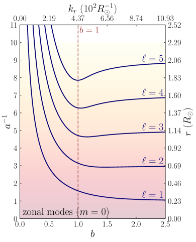
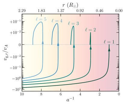
This is approximately equal to the critical magnetic field strength derived in Fuller et al. (2015), although conceptually different. For , we find numerically that the incoming wave approaches the cutoff height from above, and approaches infinite wavenumber before reaching a turning point (as can be seen in Figure 2). However, for all other values of , we find that the incoming wave first refracts outwards before approaching the cutoff height from below.
In addition, for each mode, there is some critical field such that, for (or ), there is no solution for a real value of . Only complex values of allow for solutions, implying (for real ) complex wavenumbers and evanescent waves similar to those discussed in Fuller et al. (2015) and Lecoanet et al. (2017). Physically, this means that modes will refract off of strong magnetic fields as discussed in the works above. This is different from the rotation problem where gravito-inertial waves can propagate at all radii where , regardless of the rotation rate.
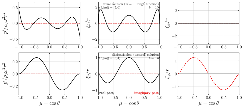
Using a relaxation method (see Appendix B.1), we solve for the eigenvalues and shown in Figure 2, and the eigenfunctions shown in the top panels of Figures 3 and 4. Because approaches a constant when approaches zero, diverges as vanishes. In most cases, an internal gravity wave branch increases in () as it is followed to higher (), until it connects to a slow magnetic branch. The wave then reaches a turning point at a maximum value of (the “critical depth”), and it is then forced to propagate back out to smaller values of (i.e., larger radii within a star) although continues to increase. The value of and the radial wavenumber then diverge at the cutoff height defined in Equation 26. This behavior is consistent with Lecoanet et al. (2017) (see Appendix A.2) who discovered the same behavior in Cartesian geometry.
| Section | ||||
| dissipationless (Section 4.1) | (Equation 26) | |||
| dissipationless (Section 4.2) | (eigenvalues of Equation 33) | |||
| dissipative real- (Section 5.2) | (Equation 44) | |||
The one exception is the case, where the wavenumber of the internal gravity wave branch directly diverges when approaching from below—there is no turning point, and no distinct slow magnetic branch. In both cases there is a maximum (minimum radius) to which the wave can propagate, and the wavenumber diverges at a cutoff height within the star. We thus find that the conclusions of Fuller et al. (2015) and Lecoanet et al. (2017) that zonal modes cannot propagate arbitrarily deep in a sufficiently magnetized star to be robust for a dipole field geometry. In Table 1, we report values of the critical depth and cutoff depths for these mode branches.
Assuming that ,he radial components of the phase and group velocities and can be specified in terms of and as
While follows the motion of the wave pattern, tracks the transport of wave energy. Figure 5 shows as a function of . Ingoing gravity waves (whose and are in opposite directions) refract at the critical depth where . They then propagate outwards as slow magnetic waves with and in the same direction, with progressively slower group velocities as they approach the cutoff height. The group velocities for modes (Sections 4.2 and 5.2) have similar behavior.
In Section 3.1, we pointed out that the Laplace tidal operator (defined in Equation 17) has branches of mostly negative eigenvalues for , which manifest as Rossby waves on the segments of the branches which are positive. However, in the magnetic problem, these branches are irrelevant when and are real, since the eigenvalues on these branches are always negative. When , this implies that () is imaginary (i.e., that the wave is evanescent). However, if is imaginary, then , and becomes
| (29) |
Equation 29 clearly has a positive on the domain of the eigenproblem, with no internal singularities at all. Sturm–Liouville theory thus implies (contrary to our initial assumption) that must be positive (see Section 3.2). This contradiction implies not only that these branches are irrelevant to the magnetogravity problem but also that the magnetogravity problem does not admit purely spatially evanescent solutions (for real ).
4.2 Tesseral and sectoral () solutions
When , the horizontal eigenfunctions (representing tesseral and sectoral modes) are simply solutions of a standard Sturm–Liouville problem with no internal singularities, and can be solved numerically using standard techniques. However, in the case, the mode and Alfvén frequencies are resonant at a critical latitude, where Equation 12 develops an internal singularity (Section 3.2). We discuss the implications of this critical latitude in the succeeding paragraphs.
In Section 3.3, it is argued (vis-à-vis power series expansion) that both the pressure perturbation and its first derivative must vanish in the vicinity of the critical latitudes . We first consider an eigenfunction with eigenvalue , and form a “Rayleigh quotient” (cf. Equation 20), but only over the portion of the domain bounded between with :
| (30) |
where the vanishing pressure perturbation and gradient justify discarding the boundary term. It is easily seen that each of the integrands above is positive-definite over the entire subdomain, and therefore .
However, one may write a similar Rayleigh quotient over the range ,
| (31) |
where it can be verified that the integrands in the numerator are now negative-definite. In Equation 31, we have similarly discarded the boundary terms—this can be done at the outer boundary so long as and its derivative are finite there. This, in turn, implies that .
Of course, by definition, an eigenfunction must have just a single eigenvalue across the entire domain. There are two ways to rectify these apparently contradictory conclusions. One possibility is that the eigenfunctions vanish outside of the critical latitudes, i.e., they are localized to a band of width , bounded by the critical latitudes on each side (as demonstrated in Section 4.1, the eigenvalues are not physical in this problem). A second possibility is that only complex values of (and hence evanescent waves) exist when the real part of is greater than unity.
In the first case, because the eigenfunction is confined to the range , we can restate the problem as a standard Sturm–Liouville problem (with no internal singularities) over this subinterval. In particular, Equation 12 can be rewritten using as
| (32) |
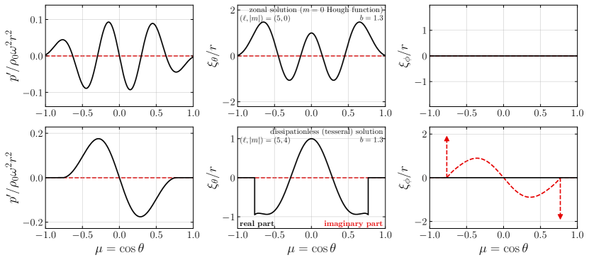
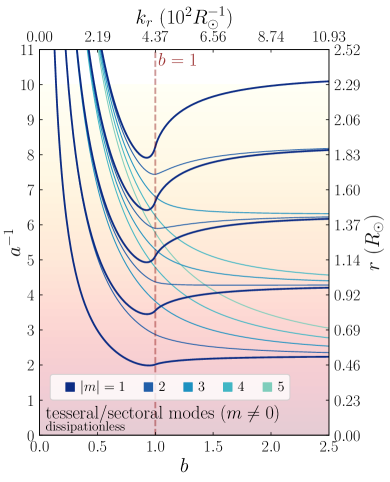
over the range . We solve for both the eigenvalues and eigenfunctions by solving Equation 12 when and Equation 32 when , again using the relaxation method (Appendix B.1). The eigenvalues for are shown in Figure 6, and example eigenfunctions are shown in the bottom panels of Figures 3 (for ) and 4 (for ), respectively. While the eigenfunctions are close to spherical harmonics for low (Figure 3), they become formally confined between the critical latitudes when , corresponding to resonances with Alfvén waves. This is in contrast to the solutions which, although also experiencing some degree of equatorial confinement, are not forced to vanish outside of the resonant latitudes.
When is large (compared to ), Equation 32 approaches
| (33) |
Equation 33 is a generalized eigenvalue problem with eigenvalues . Therefore, we see that approaches a constant cutoff value in the large limit—in other words, when approaching some cutoff value from either above or below, diverges. Moreover, since Equation 33 does not depend on , only depends on the specific solution of Equation 33 which is approached by a given branch. Therefore, is a function of , which defines the number of nodes possessed by the generalized Legendre operator. The cutoff values roughly lie between the cutoff values (defined in Equation 26), which do not follow the same pattern (see Figure 6). Table 1 reports the eigenvalues of Equation 33, which give the cutoff depths for these mode branches (as well as the critical depths ).
Another very important implication of Equation 32 is that the branches cannot extend to arbitrarily large , i.e., in a sufficiently magnetized star, propagating modes cannot extend arbitrarily deeply. When compared to Equation 18, the differential operator which appears in Equation 32 has everywhere on the domain, implying that , i.e., cannot be infinity for any finite . Furthermore, because the differential operator in Equation 33 (the large- limit of Equation 32) has and everywhere on the domain, the Rayleigh quotient (Equation 20) still implies that (in the large- limit) strictly, so long as somewhere on the domain. As this is guaranteed to be the case for any perturbation for which (since it must vary from its boundary values ), may not approach infinity even in the limit that does. If we consider the second possibility discussed above, that becomes complex, the waves become evanescent at large values of , meaning they no longer propagate. This extends the conclusions of Fuller et al. (2015) and Lecoanet et al. (2017) to the general case that propagating magnetogravity waves cannot exist arbitrarily deeply in a magnetized-enough star.
However, the localized nature of the pressure perturbations of the modes has important implications for the other perturbations (which also vanish outside of the critical latitudes, by Equations 11). For example, since the leading-order dependence of the eigenfunction near the singularity is quadratic (Section 3.3), the discontinuity of across the critical latitudes implies via Equation 11b that the value of is discontinuous. The fact that behaves as a step function near the singularity further implies (by the continuity equation) that contains a delta function at the critical latitude. This behavior is discussed in depth in Goedbloed & Poedts (2004), and we comment further on this behavior in Section 4.3.
Because of the singular denominator factors in and implied discontinuous eigenfunctions, it is important to consider that even infinitesimally little viscosity/Ohmic diffusivity can induce finite damping as well as global changes to the eigenfunctions. We further discuss these effects in Section 5. Nevertheless, the dissipationless solutions provide some analytic insight to qualitative features that they share with dissipative solutions to the magnetogravity wave problem.
4.3 Alfvén wave solutions
In Sections 3.3 and 4.2, we performed a power series expansion to probe the behavior of the perturbations around the critical latitude and solved for the solutions. However, as a second-order differential equation, one naïvely expects there to be two linearly independent solutions. More formally, when performing a Frobenius expansion, one obtains an indicial equation which can be solved to yield two solutions for the power law dependence of the solution very near the singularity (as in Section 3.3). When these two values are not separated by an integer, one immediately obtains these two linearly independent solutions.
However, the values of the indicial root found in Section 3.3 are separated by an integer, so a Frobenius expansion in is not particularly helpful in the search for the other solution. Instead, by substituting Equations 11a and 11c into the continuity equation (Equation 10a), solving for in terms of , and then substituting the result into the momentum equation (Equation 10c), one obtains
| (34) |
where
| (35) |
A power series expansion of the form
| (36) |
gives an indicial equation which has a double root at , consistent with the results of Goedbloed & Poedts 2004 on a similar magnetohydrodynamic problem (see their Section 7.4).
Hereafter, for illustrative purposes, we focus on the restricted problem over the interval in order to focus on the critical latitude at (this is justified in Section B.1). The choice of gives a single everywhere-finite solution which can be called . In this case, a second linearly independent solution is given by
| (37) |
which contains a logarithmic divergence at the critical latitude. Goedbloed & Poedts 2004 show that, while the coefficient may differ on either side of the singularity, the coefficient in front of may not. The general solution for is thus given by
| (38) |
where is the Heaviside step function. Note that that the presence of three undetermined coefficients , , and constrained by only two boundary conditions implies a continuous spectrum of modes. This is a well-established consequence of singularities in differential equations, especially those corresponding to Alfvén resonances in plasma physics (Appert et al., 1974; Poedts et al., 1985; Rauf & Tataronis, 1995; Appert et al., 1998; Widdowson et al., 1998; Rincon & Rieutord, 2003; Goedbloed & Poedts, 2004; Reese et al., 2004; Pintér et al., 2007; Loi & Papaloizou, 2017). Physically, the continuous Alfvén spectrum arises out of a lack of discretization in the direction, associated with mode localization in geometries with field/plasma inhomogeneity.
In the treatment in this work, we do not explicitly impose boundary conditions in the radial direction. However, doing so would discretize the allowed values of both for the global modes and the Alfvén waves (see, e.g., Loi & Papaloizou, 2017). Alfvén resonances can exist whenever , i.e., . The continuum Alfvén spectrum therefore occupies all frequencies with (i.e., every point to the right of in Figure 6). In practice, because each field line has a discrete spectrum of Alfvén waves (which are analogous to oscillations on a closed loop), a real global mode resonates with the Alfvén spectrum at only a finite (but large) number of locations (Loi & Papaloizou, 2017).
In problems possessing even vanishingly small amounts of dissipation, the Alfvén continuum has important implications both for the global forms of the eigenfunctions and wave damping. Hoven & Levin (2011) note that any dissipation couples fluid displacements across flux surfaces, destroying the continuum nature of the Alfvén spectrum (see Section 6.1). In Section 5, we find that including dissipation produces discrete spectra for which only a specific linear combination of and are truly eigenfunctions.
Because Alfvén waves are not associated with a pressure perturbation, the Lagrangian temperature perturbation vanishes and therefore does not produce bulk brightness fluctuations which would be asteroseismically detectable in the light curve (Houdek & Dupret, 2015).It may be possible to observe their signature in surface velocity fluctuations, if the waves do not damp before reaching the surface.
5 Oscillation modes with dissipation
So far, we have considered the mathematical problem where we have formally set all dissipation to zero. In this Section, we consider the important role played by even small amounts of dissipation in shaping the horizontal structure of magnetogravity modes.
As discussed in Section 4.3, the magnetogravity problem possesses a continuum of Alfvén modes, each localized to a magnetic field line. Adjacent Alfvén modes will oscillate at slightly different frequencies, corresponding to the slightly different Alfvén frequencies of their field lines. This quickly leads to a dephasing process called “phase mixing,” a kind of quasi-damping which, while formally reversible in ideal magnetohydrodynamics, leads to finite energy damping under any (arbitrarily small) amount of dissipation. Interestingly, this energy damping approaches a finite value in the limit of even a vanishingly small dissipation, meaning that its role cannot be ignored even in stars where dissipative processes are usually considered to be negligible. For further discussion of phase mixing and its associated energy dissipation, see Goedbloed & Poedts (2004).
If dissipation, in the form of fluid viscosity and Ohmic diffusion, are included, the linearized horizontal momentum and induction equations are modified to
| (39a) | |||
| (39b) | |||
where we continue to assume the hierarchy of variables described in Section 2.1 (including taking ). In Equations 39, and denote the kinematic viscosity and magnetic diffusivity, respectively. We note in passing that the latter is expected to dominate the overall dissipation, but that both terms have a similar impact on the solutions.
where is given by
| (41) |
where
| (42a) | |||
| (42b) | |||
In deriving Equations 40 and 41, we have assumed that . Note that, because the effect of is to shift the poles slightly off of the real line into the complex plane, the exact form of does not matter, and it suffices to take it to be a small, real constant. Moreover, since dissipation is most important near the critical latitudes , both terms scale roughly as in the most affected regions.
Overall, the operator then takes the new form
| (43) |
where encodes the dissipative processes in the problem, and “softens” the singularity.
We note in passing that terms dependent on the horizontal field may be significant at the critical latitudes where dissipation is expected to be most important. The inclusion of such terms introduces higher-order horizontal derivatives to the linearized equations and greatly increases their complexity. Nevertheless, we expect that the parameterization above in terms of will still physically select the right branch of solutions, in the limit of small dissipation. In Section 6.1, we comment further on the importance of such terms near the critical latitudes.
In the following subsections, we present numerical solutions for the dissipative magnetogravity eigenproblem (details in Appendix B.2). Section 5.1 considers modes with real but complex , i.e., possibly spatially evanescent modes, and Section 5.2 considers modes with real radial phase velocity (approximating the case of propagating waves). We will show that, while the analysis of Section 4.2 provides insights into realistic modes, the presence of dissipation introduces notable deviations from the idealized behavior.
5.1 Numerical solutions of the evanescent branch
We first consider the case where is real but is allowed to be complex (i.e., allowing solutions to be spatially evanescent). This corresponds to fixing to be real but allowing to be complex. As described in Appendix B.2, we solve for the eigenfunctions of the operator in Equation 43 up to (using ) while allowing the complex argument of to vary. For consistency, we search for only solutions with , although each such evanescent branch is accompanied by a conjugate branch of solutions.
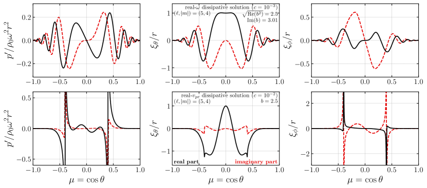
The eigenvalues are shown in Figure 7 as a function of . When (i.e., weak magnetic fields), the singularity does not lie on the domain and dissipation does not play a major role. For decreasing values of , approaches a real number, as expected, and the solutions are nearly identical to those discussed in Section 4.2.
However, for , there are significant qualitative differences between the discontinous solutions of Section 4.2 and the dissipative solutions. Even in the limit of , the imaginary part of does not correspondingly vanish, although (as we discuss below) its limiting value is sometimes quite small. This implies that the corresponding eigenfunctions are still “smoothed” with respect to the discontinuous solutions even in the limit.
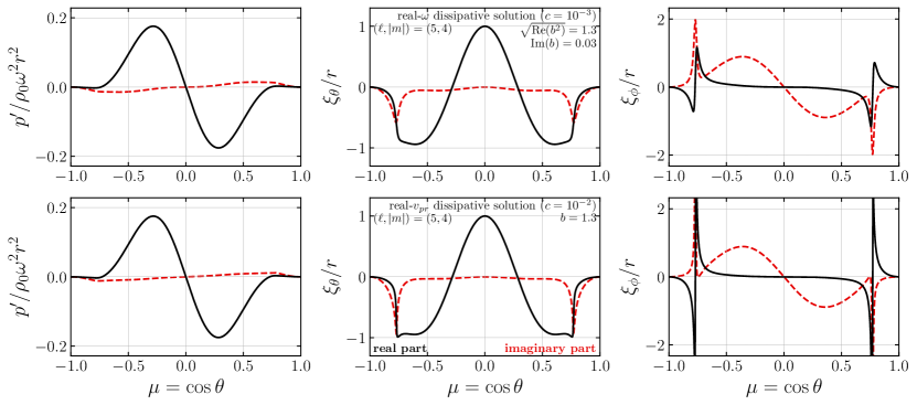
For some branches of modes, there is a range extending from to some intermediate value of where is small when . In these intermediate ranges, the real parts of , , and strongly resemble smoothed versions of the discontinuous solutions described in Section 4.2 (e.g., the top panel of Figure 8). In particular, has a smoothed step-like jump across the singularity, and retains a smoothed, but narrow, peak there. Interestingly, the imaginary part of approaches the logarithmic Alfvén “spike” solutions described in Section 4.3—the numerical solution is thus a close approximation of a superposition of these two solutions predicted in Section 4.3. These solutions can be visualized as equatorially focused magnetogravity modes which oscillate out of phase with an Alfvén mode. This closely resembles the example shown in Figure 11.2 by Goedbloed & Poedts (2004) (in a similar magnetohydrodynamic problem), as well as the numerical results of Lecoanet et al. (2022). We emphasize that, because the imaginary part of does not approach zero in the limit, the “smoothing” does not go away even in this limit. It appears that the size of the intermediate range of for which is small appears to increase with for fixed . However, the origin of this trend is so far unclear.
In all branches, for large enough , the imaginary part of found by the solver becomes large, and dips as the solver follows an evanescent branch deeper into the star. At large , all of the evanescent mode branches we solve for approach (i.e., ) such that waves radially decay in the same direction as they travel. In this regime, the eigenfunctions approach horizontally traveling waves which propagate away from the equator (e.g., top panel of Figure 9), as shown by the relative phases of the real and imaginary eigenfunctions. The conjugate branches are expected to have the opposite behavior, with the eigenfunctions approaching horizontally traveling waves which propagate toward the equator. Note that, because the values of (and therefore ) for these equator-ward and pole-ward traveling solutions are complex conjugates of each other, they exponentially decay in radius in opposite directions, and it is generally not possible to superpose them to form a wavefunction which is a horizontal standing wave at all radii.
Overall, the behavior at is very complex and difficult to characterize from first principles. Branches often have multiple “kinks” in addition to the initial one at characterizing the transition from propagation to evanescence. We suspect these kinks are related to avoided crossings between different evanescent branches of magnetogravity waves.
However, these branches represent modes that are evanescent on short length scales, implying very little wave energy propagates to larger depths. Hence, it seems clear that in the dissipative case, there are no propagating mode branches which extend arbitrarily deep into the star. This extends the two-dimensional results of Lecoanet et al. (2017) to non-axisymmetric modes. Physically, evanescent waves indicate the presence of either total internal reflection or (in this case) refraction. Unless the radial extent of the core is , the wave power transmitted by these evanescent waves through the core is vanishingly small, and conservation of energy thereby enforces that the rest of the energy (which is the vast majority) be converted into some kind of outgoing propagating wave (Section 5.2).
5.2 Numerical solutions of the propagating branch
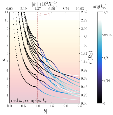
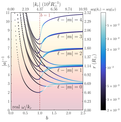
It is natural to search for solutions where waves are purely propagating (real ) but is complex (corresponding to decay). However, we find that our relaxation approach is unable to solve this particular problem formulation. Instead, we consider the case where the radial phase velocity is real, which is equivalent to taking to be real (placing the singularity as close to the real line as possible), but allowing to be complex (i.e., so that ). The eigenvalues for these calculations are shown in Figure 10.
Interestingly, in this formulation, the eigenvalues have similar qualitative behavior to discontinuous case in Figure 6. They reach some maximum at , at which point the waves turn and propagate outwards onto a slow magnetic branch which asymptotes to a finite cutoff height at infinite wavenumber. This corroborates the basic picture that propagating modes with real (or nearly real) and cannot exist in a strongly magnetized star, and that gravity waves are converted to slow magnetic waves by strong magnetic fields. Table 1 reports the critical and cutoff depths and for these solutions.
However, there are some interesting features unique to this problem, which were unanticipated by the discontinuous solutions. First, the “cutoff” values of where the wavenumbers diverge are approximately
| (44) |
This deviates from the expected cutoff heights for modes, which are the solutions to Equation 33 and lie close to even numbers rather than odd numbers. The modes have (Figure 2), offset by (in inverse depth) for the same values of . This should not be too surprising because, at , the mode eigenfunctions are very different in each case. The modes described here gain substantial complex parts (unlike the modes), and logarithmic “spike” features appear in the real part of , as shown in the bottom panel of Figure 9.
Figure 10 also shows that the imaginary components of and are largest for slightly larger than unity, reaching up to in the case. For larger values of , the complex arguments of and appear to decrease to roughly constant values of . However, due to numerical difficulty, we are unable to confirm this behavior for or much lower values of .
At values of just above unity, the eigenfunctions behave similarly to the discontinous solutions, with a sharp peak in and a discontinuity in at the critical latitude (Figure 8). In the dissipationless solutions (Section 4.2), we assumed that a given mode oscillates entirely in phase (i.e., each perturbation was either totally real or totally imaginary). For dissipative modes with only slightly larger than , this is still true—for example, for the mode at (lower panels of Figure 8), the delta function feature in oscillates in phase with the bulk oscillation between the critical latitudes (both are imaginary). However, at higher values of (lower panels of Figure 9), the sharp/discontinuous features oscillate out of phase with the bulk oscillation (e.g., the delta function in becomes real). The spike in (which occurs on the slow magnetic branch) coincides with a transition between these two regimes. This latter behavior is not captured by the non-dissipative solution, which assumes that and are purely real. It is thus unsurprising that the cutoff depths predicted by the non-dissipative solution (Section 4.2) do not coincide with those predicted by Equation 44.
For increasingly small values of , the spike features of the eigenfunctions at the critical latitudes become increasingly sharp and narrow. This makes calculating the eigenfunctions increasingly numerically challenging for smaller viscosities (we have chosen here). Decreasing from this value appears to steadily decrease for small values of , but only marginally for large values of . We suspect this is due to the finite damping rates that persist at vanishing viscosities/diffusivities for waves with these sorts of internal singularities, as discussed earlier. If true, the upward-propagating branch would also be radially evanescent: this complicates the energetic argument that all initially ingoing wave power must be carried by out by the upward-propagating branch rather than the ingoing evanescent one described in Section 5.1. However, since in this case the damping rate remains finite, we believe it is most likely that the wave energy be dissipated on the upward-propagating branch, rather than transmitting through the core. Moreover, as on this branch, upward-propagating waves will eventually attain high enough wavenumbers that they should be efficiently damped by even arbitrarily small dissipation : the argument that the wave energy is dissipated in the upward-propagating branch would then be the same as previous.
6 Further remarks
6.1 Behavior of the wavefunctions near the equator and critical latitudes
A primary assumption of our analysis is that perturbations vary much faster in the radial direction than the horizontal direction. This allowed us to effectively decouple the radial dependence of the mode from the horizontal dependence, and solve the latter independently as a two-dimensional problem over the sphere. The problem then reduces to a more tractable one-dimensional eigenproblem by making an assumption that the equilibrium field is axisymmetric (although some analytical insight is still available if this assumption is relaxed; see Section 6.3). For gravity modes at zero field, the ratio of is large, and this assumption is very reasonable. This assumption has also been instrumental in defining a hierarchy of variables whereby buoyancy and magnetism contribute at similar strengths to mode restoration (via Equation 3), and that dominates the magnetic interaction. However, this hierarchy can be subverted in a few ways.
First, in regions where the magnetic field is nearly horizontal, , and the magnetic interaction is no longer dominated by the radial part. The other magnetic terms become comparable when , which is when . For a dipole field, this occurs in a very narrow band around the equator with angular extent . It is possible that mode confinement between the critical latitudes found in our work may “funnel” refracted magnetogravity waves into radially propagating solutions which may produce detectable surface power in outgoing magnetogravity waves. We further investigate such equatorially confined magnetogravity waves in Appendix C. While such waves may exist, they have large horizontal wavenumbers and very large radial wavenumbers, so they may be difficult to observe.
The usual hierarchy can also be subverted very near the critical latitudes, where the solutions described in this work attain very sharp horizontal features. More specifically, our solutions predict that has a discontinuity and is a delta function according to the solutions in Section 4.2. While the presence of dissipation (Section 5) may smooth these sharp features somewhat, the sharpness of the features is still cause for concern in realistic stars where these effects are small. As in the example above, the terms will become important near the critical latitude and can regulate the singularity in our equations.
Now assuming a WKB approximation in both the radial and horizontal directions and a purely poloidal field (), the horizontal momentum equations become
| (45) |
where we have ignored the pressure term (note that the Alfvén waves which cause the sharp features at the critical latitudes cannot be restored by pressure).
Keeping the dominant terms (and still assuming , ),
| (46) |
Because the left-hand side of Equation 46 is close to zero near the critical latitude, we can perform a Taylor expansion in the horizontal direction:
| (47) |
where is the horizontal angular distance from the resonance point where . Here we have assumed that the displacements vary on an angular length scale such that . Appendix D solves for the “wavefunction” more precisely.
From Equation 47, we then see that the horizontal field terms terms become important when
| (48) |
However, since typically,
| (49) |
for a large-scale (e.g., dipole) magnetic field. Therefore, near the critical latitudes, we expect that the wavefunction will vary over an angular scale
| (50) |
This angular scale also naturally appears in Appendix D, where it describes the angular wavenumber of Alfvén waves near the critical latitude. Note that, because magnetogravity waves with have , they cannot couple to Alfvén waves, which are purely toroidal (i.e., ; Loi & Papaloizou, 2017). This physically explains why sharp fluid features near critical latitudes do not appear in our solutions (Section 4.1), or earlier two-dimensional solutions (Lecoanet et al., 2017).
Physically, the Alfvén and magnetogravity waves, which are decoupled in the dispersion relation of Equation 3, may become strongly coupled in a narrow band due to additional small terms left out of Equation 3. Because the Alfvén waves are expected to have angular scales due to the effect of the horizontal field, coupling between Alfvén and magnetogravity waves should also occur within of a critical latitude (due to geometric overlap). This coupling may allow a small amount of gravity wave power to be converted into outgoing Alfvén waves. These Alfvén waves would then propagate along a closed field line, eventually curving back inwards to the critical latitude on the opposite hemisphere of the star. Here, they could be converted back into outgoing gravity waves, potentially allowing for some wave power to escape the core. This possibility could be investigated with numerical simulations.
Additionally, the presence of shear stress would also cause quantifiable departures from the horizontal mode structure derived in this work. While plasmas do not generally have shear restorative forces, Hoven & Levin (2011) argue that tangling in the equilibrium magnetic field at small scales can produce a small effective shear modulus. We investigate this possibility further in Appendix E, finding that it causes the wave function to have an Airy function horizontal dependence near the critical latitude.
Out of these effects, it is most likely that the horizontal field terms have the largest impact on the mode structure (i.e., as given by Equation 50 most accurately characterizes when our solutions break down). Both dissipation and shear stress (due to, e.g., tangling) are likely to be small in real stars, but any physical equilibrium fields must have horizontal magnetic fields .
In general, the importance of horizontal-field terms near the equator and critical latitudes strongly suggests that a search for global solutions with those terms included is the natural next step for accurately characterizing strong-field modes. However, the solutions become non-separable in the radial and horizontal directions, and a solution of the full, coupled partial differential equations would be necessary. A global treatment of magnetogravity modes dramatically increases the complexity of any numerical mode calculations, but is likely to reveal important (and hard to predict) departures from a separable treatment (as it has in eigenmode problems in differentially rotating planets, e.g., Takata & Saio, 2013; Dewberry et al., 2021). While we believe our solutions to capture the basic behavior of the waves, the effects of horizontal magnetic fields discussed here are likely to be the more important effect in real stars, and should be examined more thoroughly in future work.
6.2 The continuum spectrum and nonharmonic solutions
In this work, we have focused on harmonic solutions with time dependence , for some global oscillation frequency . However, the unusual nuances introduced by the internal singularity suggest more general approaches may be appropriate. For example, standard Sturm–Liouville theory only ensures that the eigenfunctions of form a basis for a real in the absence of internal singularities. Thus, while we have mostly discussed the discrete spectrum of eigenfunctions of , it is not guaranteed that an arbitrary perturbation can be decomposed into them, both because is not necessarily real and because different modes at the same radius are eigenfunctions of different differential operators (i.e., for different ). In general, the continuous spectrum of Alfvén waves (i.e., Section 4.3) plays a major role.
Similar frequency-dependent internal singularities often appear in problems related to differentially-rotating fluids. In such problems, authors such as Burger (1966) and Balbinski (1984) apply more general Laplace transform techniques involving contour integrals to solve for the time dependence of possible solutions. Specifically, Balbinski (1984) find that the continuum spectrum in a differentially-rotating cylinder corresponds to perturbations which oscillate periodically and also decay as a power law in time. In those “quasi-modal” solutions, the oscillation frequency depends on position, and hence the solutions are not separable in space and time.
Levin (2007) and Hoven & Levin (2011) intuitively explain the origin of such non-exponential time dependence in the context of the coupling of a magnetar crust mode to an Alfvén continuum in the magnetar bulk. In a toy model analogous to this problem, a “large” oscillator (the crust mode) couples to a dense collection of “small” oscillators (the Alfvén modes). In our case, the “large" oscillator would be an ingoing gravity wave. At early times, the large oscillator’s amplitude exponentially decays as energy is distributed among the small oscillators. However, the time dependence transitions to algebraic decay to a finite, nonzero amplitude driven by coherent driving from small oscillators at the edges of the continuum. In the presence of dissipation, such edge modes retain energy for much longer than modes in the interior of the continuum. It is unclear how these edge modes manifest in the simplified model of magnetogravity waves presented in this work.
Interestingly, Boyd (1981) note in their Appendix B that the decomposition of perturbations into either real-eigenvalue continuum modes or complex-eigenvalue discrete modes are equivalent and complementary approaches. The eigenfunctions of the modes may diverge at some points, similar to an Alfvén wave confined to a single field line. However, a superposition of a continuous spectrum of modes can produce a finite-valued function. Hence, examining single continuum modes can be misleading, but they can be superposed to produce unusual decay behavior as in Balbinski (1984). In future work, application of these insights to the magnetogravity wave problem may shed more light on what to expect in real stars, including the possibility of quasi-modes with non-harmonic time dependence.
6.3 Magnetogravity waves in general geometries
In this work, we have focused on dipolar magnetic field configurations whose radial components have angular dependence (Equation 9). However, many real stars have more complex field morphologies (Maxted et al., 2000; Tout et al., 2004; Donati & Landstreet, 2009; Kochukhov et al., 2010; Szary, 2013; Kochukhov & Wade, 2016). In this Section, we generalize some of the arguments made in Section 4 to more general magnetic fields of the form
| (51) |
where is a dimensionless function describing the horizontal dependence of the field. As in Section 2.3, we use a WKB approximation such that terms dependent on the horizontal component of the field are small and can be dropped. Without loss of generality, we can rescale and so that the maximum of on the sphere is .
The general problem can be non-dimensionalized in the same way as described in Section 2.2. In particular, we still define and as in Equations 5 and 6, but interpreting as the maximum Alfvén speed at a given radius (which no longer necessarily occurs at the poles). Via Equations 2, the perturbations are given by
| (52a) | |||
| (52b) | |||
| (52c) | |||
where we have defined the horizontal gradient,
| (53) |
with the factor of excluded.
We see that Equation 54 can be viewed as a partial differential equation to be solved over a sphere of radius (i.e., Equation 54 can be rewritten without after defining some ). In other words, the depth parameter parameterizes the effective “curvature” of the spherical domain over which the horizontal equations are to be solved. Since we have not assumed a specific magnetic field geometry here, the form of the differential eigenproblem in Equation 4 is generic. In the case of an axisymmetric field, the two-dimensional angular differential operator in Equation 54 can be reduced to a differential operator in only (recovering, e.g., Equation 12, for a dipole field).
Equation 52b can be rearranged to
| (55) |
We therefore see that, so long as is finite, along any critical surface () as long as is real.
The vanishing directional derivative of across the critical surface generalizes an analogous result in Section 3.3 for the dipole geometry. Physically, this result simply reflects that, at the site of an Alfvén resonance, magnetic tension completely accounts for the (horizontal) restoring force of the mode, and the pressure perturbation makes no contribution. This fact was also used in Section 4.2 to show that dissipationless solutions must vanish outside of the critical latitudes.
We can perform a similar analysis as in Section 4.2 by multiplying Equation 54 by and integrating over the region of the sphere where (i.e., where ), denoted by :
| (56) |
The second term becomes
| (57) |
where we have first integrated by parts, and then applied the divergence theorem to the first term ( denotes the boundary of , is an angular line element, and points out of ). If the first (boundary) term in Equation 57 vanishes, then
| (58) |
generalizes Equation 30. However, this process can be repeated for , the region where , to obtain
| (59) |
Since may only have one sign or another for a given global mode, we see that modes for which and are both real (i.e., propagating and non-decaying) will be localized to the region where in the case when the boundary term in Equation 57 vanishes. This condition will be satisfied when the complex winding number enclosed by is nonzero, since on . This argument generalizes the result described in Section 4.2 that propagating, non-decaying modes in the dipole geometry must be localized between the critical latitudes.
6.4 Stable modes in convective regions
Standard mixing-length theory assumes a slight superadiabatic temperature gradient such that in convective zones. While modes in non-rotating, non-magnetized stars are only present in stably stratified (radiative) regions, Lee & Saio (1997) show that buoyancy-restored oscillatory modes (real ) can be stabilized even in convective regions () by sufficiently high rotation. In particular, when , the coefficient functions which appear in the Laplace tidal operator (Equation 17) are no longer strictly positive, and it will possess negative eigenvalues . In this case, becomes imaginary, and there exist solutions to when is also imaginary. While standard modes under strong rotation tend to be localized to the equator, these rotationally stabilized convective modes are instead localized near the poles (Lee & Saio, 1997).
However, the same argument can be applied to the magnetogravity problem, and gives meaning to the negative branches of eigenvalues implied by Equation 12. In particular, like , the operator (Equation 13) also contains coefficients which switch signs over the domain. In this formalism, for oscillatory solutions with real , becomes imaginary, and one instead must solve
| (60) |
where now the (negative) eigenvalues of must satisfy
| (61) |
In the case of no buoyancy () and relaxing the Boussinesq assumption, convective regions are expected to sustain standard magnetohydrodynamic waves (Shu, 1991). On top of these modes, the aforementioned negative eigenvalue branches hint at the existence of buoyancy-restored oscillations in convective regions which are stabilized by magnetic forces. By a similar argument as made in Section 4.2, Equation 60 implies that such modes would be exactly localized outside (rather than inside) the critical latitudes. Moreover, while they require , there is no formal upper limit on the magnetic fields at which they can exist, meaning they may exist in the convective cores of strongly magnetized stars.
While the analogy to rotationally stabilized convective modes seems obvious, we note the magnitude of the Brunt–Väisälä frequency is typically extremely close to in convective zones, owing to the extremely efficient mixing caused by the convective instability. Note that this feature is not unique to the magnetogravity problem, and would also be true for the rotational problem considered by Lee & Saio (1997). This appears to violate a fundamental assumption of our analysis that is large, or at least implies that stable convective oscillations which can accurately be described by our formalism must be of very low frequency. Therefore, we strongly caution against using the formalism in this work to make quantitative (or even strong qualitative) predictions about the properties of these modes. More detailed analyses relaxing this assumption are necessary to characterize these modes accurately (if indeed they exist).
7 Summary
In this work, we have characterized the pulsation modes of a spherically symmetric, stratified stellar structure with a strong dipole magnetic field. We focus on radiative zones with large Brunt–Väisälä frequencies such that magnetogravity waves have short radial wavelengths. We have assumed that
-
•
the radial wavelength is everywhere much smaller than both the stellar structure length (the radial WKB approximation) and the horizontal wavelength (i.e., the wavevector is primarily radial),
-
•
oscillations are incompressible and adiabatic,
-
•
perturbations to the gravitational potential can be ignored (Cowling), and
- •
Our chief conclusions are as follows:
-
1.
Propagating zonal () magnetogravity modes merge at a finite field with a branch of slow magnetic waves whose wavenumbers diverge at a finite cutoff radius. Their horizontal eigenfunctions are Hough functions for a dipolar magnetic field. Hence, ingoing gravity waves are converted into slow magnetic waves at a critical magnetic field strength similar to that derived in Fuller et al. (2015). Above this field strength, the modes become evanescent and cannot propagate. This is in agreement with the results of Lecoanet et al. 2017 in a similar geometry.
-
2.
Propagating sectoral and tesseral () modes also merge with branches of slow magnetic waves whose wavenumbers diverge at a cutoff radius within the star. Like modes, ingoing gravity waves cannot propagate above a critical magnetic field strength, and are instead converted to outgoing slow magnetic waves. For strong fields and large wavenumbers, the modes are closely confined to the equator, and are bounded by sharp features in the fluid displacement profile at critical latitudes where the wave frequency is resonant with Alfvén waves.
-
3.
Even vanishingly small dissipation can cause qualitative deviations from the problem where dissipation is formally set to zero. This can be heuristically understood because viscosity allows for interaction between magnetogravity waves and the continuous Alfvén wave spectrum. However, even for finite dissipation, the conclusion that sufficiently high magnetic fields will destroy all propagating magnetogravity modes is robust.
-
4.
Near the critical latitudes and equator, magnetic tension terms associated with the horizontal field are likely to affect the mode structure significantly. Thus, a global solution which includes such terms is necessary to confidently characterize the mode structure very near these regions. We speculate that such an analysis might reveal that an observable amount of wave power may be able to escape a strongly magnetized stellar core through coupling with Alfvén waves (at critical latitudes) or extremely localized magnetogravity waves (near the equator).
Our analysis reinforces conclusions from earlier studies that strong magnetic fields should convert gravity waves into slow magnetic waves that damp within stellar interiors, causing magnetic fields to suppress the amplitudes of gravity modes in red giant stars (Fuller et al., 2015; Stello et al., 2016b). However, it may remain possible that higher-order WKB terms (neglected in our analysis) or modes with non-harmonic time dependence (Section 6.2) could allow for some signatures of mixed modes in observed power spectra as claimed by Mosser et al. (2017). More effort accounting for these effects will be required to robustly predict the magnetogravity pulsation spectra of stars with strong magnetic fields.
Acknowledgements
We thank Daniel Lecoanet, Yuri Levin, Sterl Phinney, Janosz Dewberry, Joel Ong, and Saul Teukolsky for their helpful advice and comments. N.Z.R. acknowledges support from the National Science Foundation Graduate Research Fellowship under Grant No. DGE-1745301. J.F. is thankful for support through an Innovator Grant from The Rose Hills Foundation, and the Sloan Foundation through grant FG-2018-10515. We thank the anonymous referee for their thorough review and helpful suggestions, which greatly improved the work.
Data Availability
The output of the oscillation mode calculations described in this work will be shared upon reasonable request to the corresponding author.
References
- Al-Gwaiz (2008) Al-Gwaiz M. A., 2008, Sturm-Liouville theory and its applications. Vol. 264, Springer
- Angel (1977) Angel J., 1977, The Astrophysical Journal, 216, 1
- Appert et al. (1974) Appert K., Gruber R., Vaclavik J., 1974, Physics of Fluids, 17, 1471
- Appert et al. (1998) Appert K., Gruber R., Vaclavik J., 1998, Technical report, Continuous spectra of a cylindrical magnetohydrodynamic equilibrium: the derivation
- Atkinson et al. (1988) Atkinson F., Everitt W., Zettl A., 1988, Differential and Integral Equations, 1, 213
- Balbinski (1984) Balbinski E., 1984, Monthly Notices of the Royal Astronomical Society, 209, 145
- Baliunas et al. (1996) Baliunas S., Nesme-Ribes E., Sokoloff D., Soon W., 1996, The Astrophysical Journal, 460, 848
- Bildsten et al. (1996) Bildsten L., Ushomirsky G., Cutler C., 1996, ApJ, 460, 827
- Boyd (1976) Boyd J. P., 1976, Ph. D. Thesis
- Boyd (1981) Boyd J. P., 1981, Journal of Mathematical Physics, 22, 1575
- Boyd (1982) Boyd J. P., 1982, Journal of Atmospheric Sciences, 39, 770
- Braithwaite & Spruit (2004) Braithwaite J., Spruit H. C., 2004, nature, 431, 819
- Brun & Browning (2017) Brun A. S., Browning M. K., 2017, Living Reviews in Solar Physics, 14, 1
- Buckingham (1914) Buckingham E., 1914, Physical review, 4, 345
- Bugnet (2022) Bugnet L., 2022, Astronomy & Astrophysics, 667, A68
- Bugnet et al. (2021) Bugnet L., et al., 2021, Astronomy & Astrophysics, 650, A53
- Burger (1966) Burger A., 1966, Journal of Atmospheric Sciences, 23, 272
- Cantiello et al. (2016) Cantiello M., Fuller J., Bildsten L., 2016, The Astrophysical Journal, 824, 14
- Chen & Lü (2009) Chen Z.-Y., Lü D.-R., 2009, Chinese Journal of Geophysics, 52, 547
- Dewberry et al. (2021) Dewberry J. W., Mankovich C. R., Fuller J., Lai D., Xu W., 2021, The Planetary Science Journal, 2, 198
- Dhouib et al. (2022) Dhouib H., Mathis S., Bugnet L., Van Reeth T., Aerts C., 2022, Astronomy & Astrophysics, 661, A133
- Donati & Landstreet (2009) Donati J., Landstreet J., 2009, arXiv preprint arXiv:0904.1938
- Dudorov & Khaibrakhmanov (2015) Dudorov A. E., Khaibrakhmanov S. A., 2015, Advances in Space Research, 55, 843
- Everitt et al. (1987) Everitt W., Gunson J., Zettl A., 1987, Zeitschrift für angewandte Mathematik und Physik ZAMP, 38, 813
- Federman (1911) Federman A., 1911, Proc. St.-Petersburg Polytech. Inst. Sect. Tech. Nat. Sci. Math, 16, 97
- Ferrario et al. (2009) Ferrario L., Pringle J., Tout C. A., Wickramasinghe D., 2009, Monthly Notices of the Royal Astronomical Society: Letters, 400, L71
- Ferrario et al. (2015) Ferrario L., Melatos A., Zrake J., 2015, Space Science Reviews, 191, 77
- Fuller & Lai (2014) Fuller J., Lai D., 2014, Monthly Notices of the Royal Astronomical Society, 444, 3488
- Fuller et al. (2015) Fuller J., Cantiello M., Stello D., Garcia R. A., Bildsten L., 2015, Science, 350, 423
- García et al. (2014) García R., et al., 2014, Astronomy & Astrophysics, 563, A84
- Goedbloed & Poedts (2004) Goedbloed H., Poedts S., 2004, Principles of magnetohydrodynamics: with applications to laboratory and astrophysical plasmas. Cambridge university press
- Goossens (1972) Goossens M., 1972, Astrophysics and Space Science, 16, 386
- Goossens (1976) Goossens M., 1976, Astrophysics and Space Science, 43, 9
- Goossens et al. (1976) Goossens M., Smeyers P., Denis J., 1976, Astrophysics and Space Science, 39, 257
- Gunson (1987) Gunson J., 1987, Proceedings of the Royal Society of London. A. Mathematical and Physical Sciences, 414, 255
- Homer (1990) Homer M., 1990, Proceedings of the Royal Society of London. A. Mathematical and Physical Sciences, 428, 157
- Houdek & Dupret (2015) Houdek G., Dupret M.-A., 2015, Living Reviews in Solar Physics, 12, 1
- Hough (1898a) Hough S. S., 1898a, Philosophical Transactions of the Royal Society of London. Series A, Containing Papers of a Mathematical or Physical Character, pp 139–185
- Hough (1898b) Hough S. S., 1898b, Philosophical Transactions of the Royal Society of London. Series A, Containing Papers of a Mathematical or Physical Character, 191, 139
- Hoven & Levin (2011) Hoven M. v., Levin Y., 2011, Monthly Notices of the Royal Astronomical Society, 410, 1036
- Kochukhov & Wade (2016) Kochukhov O., Wade G., 2016, Astronomy & Astrophysics, 586, A30
- Kochukhov et al. (2010) Kochukhov O., Lundin A., Romanyuk I., Kudryavtsev D., 2010, The Astrophysical Journal, 726, 24
- Kulkarni & Thompson (1998) Kulkarni S., Thompson C., 1998, Nature, 393, 215
- Lecoanet et al. (2017) Lecoanet D., Vasil G. M., Fuller J., Cantiello M., Burns K. J., 2017, Monthly Notices of the Royal Astronomical Society, 466, 2181
- Lecoanet et al. (2022) Lecoanet D., Bowman D. M., Van Reeth T., 2022, Monthly Notices of the Royal Astronomical Society: Letters, 512, L16
- Lee & Saio (1997) Lee U., Saio H., 1997, The Astrophysical Journal, 491, 839
- Levin (2006) Levin Y., 2006, Monthly Notices of the Royal Astronomical Society: Letters, 368, L35
- Levin (2007) Levin Y., 2007, Monthly Notices of the Royal Astronomical Society, 377, 159
- Li et al. (2022) Li G., Deheuvels S., Ballot J., Lignières F., 2022, 30 to 100-kG magnetic fields in the cores of red giant stars, doi:10.48550/ARXIV.2208.09487, https://arxiv.org/abs/2208.09487
- Liebert et al. (2003) Liebert J., Bergeron P., Holberg J., 2003, The astronomical journal, 125, 348
- Loi (2020a) Loi S. T., 2020a, Monthly Notices of the Royal Astronomical Society, 493, 5726
- Loi (2020b) Loi S. T., 2020b, Monthly Notices of the Royal Astronomical Society, 496, 3829
- Loi & Papaloizou (2017) Loi S. T., Papaloizou J. C., 2017, Monthly Notices of the Royal Astronomical Society, 467, 3212
- Loi & Papaloizou (2018) Loi S. T., Papaloizou J. C., 2018, Monthly Notices of the Royal Astronomical Society, 477, 5338
- MacGregor & Rogers (2011) MacGregor K. B., Rogers T., 2011, Solar Physics, 270, 417
- Maeder & Meynet (2005) Maeder A., Meynet G., 2005, Astronomy & Astrophysics, 440, 1041
- Mathieu (1868) Mathieu É., 1868, Journal de mathématiques pures et appliquées, 13, 137
- Mathis & De Brye (2011) Mathis S., De Brye N., 2011, Astronomy & Astrophysics, 526, A65
- Mathis et al. (2021) Mathis S., Bugnet L., Prat V., Augustson K., Mathur S., Garcia R. A., 2021, Astronomy & Astrophysics, 647, A122
- Maxted et al. (2000) Maxted P., Ferrario L., Marsh T., Wickramasinghe D., 2000, Monthly Notices of the Royal Astronomical Society, 315, L41
- Mosser et al. (2012) Mosser B., et al., 2012, Astronomy & Astrophysics, 537, A30
- Mosser et al. (2017) Mosser B., et al., 2017, Astronomy & Astrophysics, 598, A62
- Pintér et al. (2007) Pintér B., Erdélyi R., Goossens M., 2007, Astronomy & Astrophysics, 466, 377
- Poedts et al. (1985) Poedts S., Hermans D., Goossens M., 1985, Astronomy and astrophysics, 151, 16
- Prat et al. (2019) Prat V., Mathis S., Buysschaert B., Van Beeck J., Bowman D. M., Aerts C., Neiner C., 2019, Astronomy & Astrophysics, 627, A64
- Prat et al. (2020) Prat V., Mathis S., Neiner C., Van Beeck J., Bowman D. M., Aerts C., 2020, A&A, 636, A100
- Prendergast (1956) Prendergast K. H., 1956, The Astrophysical Journal, 123, 498
- Press et al. (2007) Press W. H., Teukolsky S. A., Vetterling W. T., Flannery B. P., 2007, Numerical Recipes with Source Code CD-ROM 3rd Edition: The Art of Scientific Computing. Cambridge University Press
- Proctor & Weiss (1982) Proctor M., Weiss N., 1982, Reports on Progress in Physics, 45, 1317
- Rauf & Tataronis (1995) Rauf S., Tataronis J., 1995, Physics of Plasmas, 2, 340
- Reese et al. (2004) Reese D., Rincon F., Rieutord M., 2004, Astronomy & Astrophysics, 427, 279
- Riabouchinsky (1911) Riabouchinsky D., 1911, L’aérophile, 1, 407
- Rincon & Rieutord (2003) Rincon F., Rieutord M., 2003, Astronomy & Astrophysics, 398, 663
- Rogers & MacGregor (2010) Rogers T., MacGregor K., 2010, Monthly Notices of the Royal Astronomical Society, 401, 191
- Schneider et al. (2019) Schneider F., Ohlmann S. T., Podsiadlowski P., Röpke F. K., Balbus S. A., Pakmor R., Springel V., 2019, Nature, 574, 211
- Shu (1991) Shu F. H., 1991, The Physics of Astrophysics: Gas Dynamics. Vol. 2, University Science Books
- Spruit (2002) Spruit H., 2002, Astronomy & Astrophysics, 381, 923
- Stello et al. (2016a) Stello D., Cantiello M., Fuller J., Garcia R. A., Huber D., 2016a, Publications of the Astronomical Society of Australia, 33, e011
- Stello et al. (2016b) Stello D., Cantiello M., Fuller J., Huber D., García R. A., Bedding T. R., Bildsten L., Aguirre V. S., 2016b, Nature, 529, 364
- Szary (2013) Szary A., 2013, arXiv preprint arXiv:1304.4203
- Takata & Saio (2013) Takata M., Saio H., 2013, Publications of the Astronomical Society of Japan, 65
- Thompson & Duncan (1993) Thompson C., Duncan R. C., 1993, The Astrophysical Journal, 408, 194
- Tout et al. (2004) Tout C. A., Wickramasinghe D. T., Ferrario L., 2004, Monthly Notices of the Royal Astronomical Society, 355, L13
- Townsend (2003) Townsend R., 2003, Monthly Notices of the Royal Astronomical Society, 340, 1020
- Townsend (2020) Townsend R., 2020, Monthly Notices of the Royal Astronomical Society, 497, 2670
- Tutukov & Fedorova (2010) Tutukov A., Fedorova A., 2010, Astronomy Reports, 54, 156
- Unno et al. (1989) Unno W., Osaki Y., Ando H., Saio H., Shibahashi H., 1989, Unno, W., Osaki, Y., Ando, H., Saio, H., & Shibahashi, H, 755
- Vaschy (1892) Vaschy A., 1892, in Annales télégraphiques. pp 25–28
- Vidotto et al. (2014) Vidotto A., et al., 2014, Monthly Notices of the Royal Astronomical Society, 441, 2361
- Wang et al. (2016) Wang H., Boyd J. P., Akmaev R. A., 2016, Geoscientific Model Development, 9, 1477
- Whittaker (1903) Whittaker E. T., 1903
- Wickramasinghe & Ferrario (2000) Wickramasinghe D., Ferrario L., 2000, Publications of the Astronomical Society of the Pacific, 112, 873
- Wickramasinghe et al. (2014) Wickramasinghe D. T., Tout C. A., Ferrario L., 2014, Monthly Notices of the Royal Astronomical Society, 437, 675
- Widdowson et al. (1998) Widdowson S., Hurricane O., Cowley S., 1998, Physics of Plasmas, 5, 1259
Appendix A Magnetogravity eigenproblems in other geometries
In this Appendix, we non-dimensionalize the fluid equations for the geometries considered by Fuller et al. (2015) and Lecoanet et al. (2017), and show that they can be interpreted as similar eigenvalue problems as considered in our work.
A.1 Fuller et al. (2015): Uniform radial field model
The model presented by Fuller et al. (2015) can be precisely reproduced by adopting a purely uniform radial magnetic field,
| (62) |
Adopting a WKB approximation in the radial direction, we can define
| (63a) | |||
| (63b) | |||
where .
While such a monopolar field is clearly unphysical, it is also a useful toy model because it retains the spherical symmetry of the zero-field problem. Therefore, its horizontal eigenfunctions are simply spherical harmonics, and its dispersion relation is
| (64) |
Equation 64 can be analytically solved for to yield
| (65) |
where it can be seen that there are no real solutions for for some critical given by
| (66) |
This is equivalent to the result originally presented by Fuller et al. (2015) that there are no propagating solutions when the magnetogravity frequency (defined in Equation 1) rises above the mode frequency. At small buoyancy or Alfvén frequencies, the two solutions for in Equation 65 approach the usual internal gravity wave and Alfvén wave dispersion relations, and remain finite. Equations 62, 63, and 64 are analogous to Equations 9, 5 and 6, and 15 in the main text.
A.2 Lecoanet et al. (2017): Multipole Cartesian geometry
Lecoanet et al. (2017) consider a Cartesian geometry with the equilibrium magnetic field configuration
| (67) |
where the oscillatory dependence in is chosen to closely mimic the dependence of a multipole magnetic field.
Define to the wavenumber which defines the periodicity of the domain, i.e., the solution is periodic in with a period ( is analogous to in the spherical problem). We can first define
| (68a) | |||
| (68b) | |||
where .
Then, following a very similar procedure to the spherical dipole problem described in the main text, the three-dimensional Cartesian problem corresponding to the field in Equation 67 can be reduced to
| (69) |
where .
In the special case that (i.e., a dipole field), the differential operator is given by
| (70) |
where . Letting be a given (negative) eigenvalue of , the dispersion relation takes the form
| (71) |
Lecoanet et al. (2017) solve the problem described above in the two-dimensional zonal case (i.e., ), taking advantage of the fact that two-dimensional incompressibility defines a “vector potential” whose direction is everywhere orthogonal to the fluid motions. They find the eigenfunctions to be Mathieu functions (Mathieu, 1868), with a branch of inward-traveling internal gravity waves refracting up into a branch of slow magnetic waves which diverge to infinite wavenumber at a finite “cutoff” radius. We reproduce this behavior in the dipole geometry for the modes (see Section 4.1).
Appendix B Numerically solving
We use a relaxation scheme to numerically solve Equations 72 and 73, following closely the procedure used by Lee & Saio (1997) and Fuller & Lai (2014) to diagonalize the Laplace tidal equation. using the C++ implementation given by Numerical Recipes (Press et al., 2007).
However, the procedures which we adopt vary somewhat for the dissipative and dissipationless cases. The numerical solution procedure for Sections 4.1 and 4.2 is summarized in Section B.1, and the procedure for Section 5 is summarized in Section B.2.
B.1 Numerical solution without dissipation
In the (Section 4.1) and (Section 4.2) cases without dissipation, little special care is required to solve the requisite two first-order differential equations. In the former case, the solutions (Hough functions) are known to be second-differentiable across the singularity. In the latter case, the problem is a standard Sturm–Liouville problem with no internal singularities. Moreover, because (Equation 13) is even with respect to , its eigenfunctions can be partitioned into even and odd parity, which is given by for and for . This known parity greatly simplifies the problem, allowing us to solve for the eigenfunctions for only rather than over the full domain.
Then, defining and as (assumed real) non-dimensionalized versions of and , our equations become
| (72a) | |||
| (72b) | |||
where the first equation follows from the component of the momentum equation (Equation 10c) and the second equation follows from the continuity equation (Equation 10a).
Starting from Legendre polynomials as initial guess, we gradually increase () from , retaining lower solutions as initial guesses for higher relaxations. Note that, in the numerical implementation, we promote to a function of , and additionally enforce (this is the standard technique for solving such eigenproblems in, e.g., Press et al., 2007). We impose boundary conditions on and at depending on parity, setting one of these variables to and the other to for normalization. Additionally, at the right boundary , we enforce that must vanish (which can be seen in its definition).
In the case, we demonstrate in Section 4.2 that eigenfunctions in the formal zero-dissipation limit are exactly localized to the band between the internal singularities at (where we have taken without loss of generality). Then we can rescale Equations 72 via to
| (73a) | |||
| (73b) | |||
over the range (i.e., ), enforcing at (see Section 4.2).
B.2 Numerical solution with dissipation
When dissipation is considered, the internal singularities are “softened” in the sense that they are shifted off of the real line. Therefore, a case-wise treatment of the singularity (as in Section B.1) is not necessary. However, in general, both the perturbations and at least one of the quantities and are complex, doubling the number of equations to be solved.
Moreover, in the dissipative case (even for arbitrarily small viscosities/diffusivities), the delta function which appears in becomes softened to a sharp peak with a finite width. Therefore, instead of solving for as a perturbation, we probe this peak by solving the complex versions of the following equations,
| (74a) | |||
| (74b) | |||
where . In Section 5.1, we pick and take and and solve for and , while varying . In Section 5.2, we pick and take and (real) and solve for and , while again varying . As in Section B.1, the first equation follows from the component of the momentum equation, and the second equation follows from the continuity equation (but in terms of different perturbations).
The evenness and oddness conditions can be applied as in Section B.1 to (which has the same parity as ) and at the left boundary . At this same boundary, we enforce (due to overall phase invariance) . Finally, at , we enforce . Equations 74 are then solved for increasingly large values of , using associated Legendre polynomials as the initial guesses.
Appendix C Tightly confined equatorial magnetogravity waves
In this Appendix, we investigate the behavior of magnetogravity waves very close to the equator (for a dipole field), where . In the following, we demonstrate in this narrow equatorial band the existence of self-consistent, propagating solutions with wavenumbers enhanced in magnitude by a factor . These solutions are not captured by the analysis in the main text, which assumed that the vertical component of the Alfvén velocity dominates the mode structure. However, the dynamics of these modes may play an important role in understanding the observable, asteroseismic consequences of strong core magnetic fields.
In this region, the assumption (used throughout this work) that the Alfvén frequency is dominated by the radial component is violated. We expect this violation to be important when
| (75) |
or in a narrow band around the equator with angular extent .
Assuming a WKB approximation in all directions, the dispersion relation for magnetogravity waves near the equator becomes
| (76) |
where now is dominated by the horizontal component. Then, solving for , we have
| (77) |
where the criterion for radial propagation is
| (78) |
Because these solutions are only accurate in an equatorial band , it follows that
| (79) |
i.e., at least one horizontal wavelength fits within this band. The criteria in Equation 78 and 79 can be combined to obtain
| (80) |
where is the critical magnetic field strength from Equation 7, but now applied to the horizontal field rather than the radial field. Therefore, such confined magnetogravity waves would remain radially propagating in roughly the same regions that magnetogravity waves throughout the rest of the star would (within a small, order-unity factor in radius).
Interestingly, when Equation 78 (for the minimum ) is combined with Equation 77 for propagating waves, we obtain
| (81) |
where we have examined the limit where (i.e., at fields much lower than the critical field, or where ). This radial wavenumber is larger than the radial wavenumber of normal, low- gravity waves by a large factor , implying that magnetogravity waves near the equator will develop very small radial wavelengths. This increased radial wavenumber appears to be qualitatively consistent with numerical simulations conducted by Lecoanet et al. (2017), which seem to exhibit such waves at locations where the radial magnetic field vanishes (see their Figure 6). However, their simulation also seems to show outgoing equatorially confined evanescent waves, whose driving we cannot explain. Moreover, due to their small spatial scale, it is unclear to us whether these modes are numerically resolved. Future work will be required to further elucidate the nature of these highly confined modes.
Note that the dispersion relation in Equation 77 implies that the group and phase velocities of these confined magnetogravity waves are in opposite directions (similar to normal, zero-field gravity waves). Because the refracted, outgoing magnetogravity wave solutions at (described in the rest of this work) have aligned group and phase velocities, this implies that such outgoing magnetogravity waves couple most efficiently to ingoing, equatorially confined magnetogravity waves (described above). This poses a challenge for equatorially confined magnetogravity waves as a vehicle for bringing wave power out of the core. Moreover, the very short wavelengths of the equatorially confined waves make them much more susceptible to damping processes. Further work may elucidate the nature of these waves, and their role in wave power transport and dissipation.
Appendix D Structure of Alfvén resonances including horizontal-field contributions to the magnetic tension
In the solutions throughout the main text, it has been assumed that the magnetic tension terms which appear in the momentum equations are dominated by the radial component (in, e.g., Equations 10). However, very near to (i.e., very near to a critical latitude), the horizontal components of the magnetic tension may become relevant. As described throughout the text (e.g., Section 6.1), sharp horizontal fluid features may appear in the vicinity of Alfvén resonances. To estimate the impact of such terms, we will make a WKB approximation in both the radial and horizontal directions (i.e., ). We further hypothesize that it still remains true that (this will set a condition for validity). For Alfvén waves, we examine the horizontal momentum equation:
| (82) |
where we have assumed a poloidal field () for simplicity. Because we are interested in the solution in the vicinity of , we can perform a Taylor expansion:
| (83) |
where , and is the critical latitude. Then Equation 82 becomes
| (84) |
where allowed us to drop the term . This becomes
| (85) |
Then, since and (since varies horizontally roughly on the order of a radian), the prefactors involving and are order-unity. Doing this more carefully for a dipole field (where and ) yields
| (86) |
Equation 86 is straightforwardly solved by
| (87) |
This complex Gaussian describes a wave whose wavelength decreases away from the critical latitude . The first wavelength occurs where , yielding a characteristic angular scale of , or characteristic angular wavenumber of (compare Equation 50). Note that this horizontal wavenumber satisfies our assumption that .
Appendix E Magnetic tangling-induced shear stress
While realistic stars do not have shear-restorative forces, Hoven & Levin (2011) argue that small-scale disordered magnetic fields (“tangling”) may introduce an effective shear stress, with characteristic wave speed . To characterize the effect that this shear modulus term has on the Alfvén waves, we can focus on the magnetic tension term in the horizontal momentum equation, which is the only other term capable of restoring torsional mode components (Loi & Papaloizou, 2017):
| (88) |
We see that Equation 88 is mathematically identical to a two-dimensional Schrödinger equation, where plays the role of the total energy, plays the role of the potential, and the small shear speed plays the role of . As noted by Hoven & Levin (2011), the effect of a small shear modulus is to transform the continuous spectrum of Alfvén waves into a discrete one (as in standard bound-state spectra of the Schrödinger equation), whose mode spacings decrease to zero in the limit where . If a WKB approximation is adopted for Equation 88 in the horizontal direction, the coupling of these discrete waves to a mode is similar to that of the continuum waves in the case. In the region where , the discrete Alfvén wave oscillates spatially very rapidly, and its overlap with a global-scale mode averages to zero. Similarly, in the region where , the wave decays very rapidly, and therefore is very close to zero. However, the solution very close to (the “classical turning point”) is known to be an Airy function of angular width
| (89) |
which sets the scale at which an interaction with a mode and Alfvén wave will be “smeared” in the angular direction, due to shear stress. Physically, the shear modulus-induced discretization of the Alfvén waves occurs because shear adds an isotropic contribution to the wave speed (so that it is not exactly zero perpendicular to the field lines), and thus couples fluid motions across field lines. This effect is likely to be small relative to similar effects associated with the horizontal component of the mean magnetic field (Section 6.1).