Human-Inspired Framework to Accelerate Reinforcement Learning

Abstract

Reinforcement learning (RL) is crucial for data science decision-making but suffers from sample inefficiency, particularly in real-world scenarios with costly physical interactions. This paper introduces a novel human-inspired framework to enhance RL algorithm sample efficiency. It achieves this by initially exposing the learning agent to simpler tasks that progressively increase in complexity, ultimately leading to the main task. This method requires no pre-training and involves learning simpler tasks for just one iteration. The resulting knowledge can facilitate various transfer learning approaches, such as value and policy transfer, without increasing computational complexity. It can be applied across different goals, environments, and RL algorithms, including value-based, policy-based, tabular, and deep RL methods. Experimental evaluations demonstrate the framework’s effectiveness in enhancing sample efficiency, especially in challenging main tasks, demonstrated through both a simple Random Walk and more complex optimal control problems with constraints.

I Introduction

Intelligent and data-driven decision-making is becoming an increasingly important part of data science. The subfield of AI concerned with how intelligent agents learn to make optimal decisions in an unknown environment from data and experience is RL. The area has flourished recently by building on advancements in deep learning that have given RL agents superb generalization abilities [1]. Deep-RL has had a huge impact in multiple areas where it has solved challenging problems, e.g., in game playing [2], financial markets [3], robotic control [4], optimal control [5], and autonomous driving [6].

A central challenge hindering RL from achieving its full potential in many application areas is that RL approaches generally need a lot of samples to learn good decision policies [7, 8, 9]. This translates to costly and time-consuming interactions with the environment, particularly in real-world scenarios like cyber-physical systems, medical applications, and robotics [10, 11]. The quest to enhance exploration and learning efficiency remains a key challenge in RL.

Most existing RL algorithms start the learning process from scratch. In particular, the agent starts exploring each environment without using any prior knowledge (there are notable exceptions; see Section V). This is fundamentally different from how humans explore and learn in new environments [12]. When tackling complex tasks, humans adopt a step-by-step approach. They break down the overarching goal into manageable short-term objectives that align with the main goal. To illustrate, consider a math teacher guiding a student. The teacher starts with basic addition, then moves to multiplication, and eventually introduces exponents. This incremental approach enhances comprehension. Similarly, RL agents facing tough challenges might benefit from mastering simpler, related tasks before tackling the primary objective, mirroring human learning principles.

Contribution: This paper introduces a framework for Teacher-Assisted exploration in RL. It systematically aids the RL agent’s learning process by providing progressively challenging auxiliary goals alongside the main goal. These auxiliary goals are incorporated by introducing an assistant reward in conjunction with the target reward, managed through an annealing function, creating a sequential progression of Markov decision processes (MDPs). The agent alternates between learning each auxiliary goal for a single iteration, leveraging the acquired knowledge to expedite mastery of the main goal. This approach eliminates the need for defining numerous separate MDPs with similar distributions. Importantly, our framework is algorithm-agnostic and compatible with various RL methods, including value-based, policy-based, tabular, and deep-RL approaches. We demonstrate its effectiveness in intuitive scenarios using tabular algorithms and validate its efficiency through extensive deep-RL experiments on control problems (refer to Section IV). The results indicate that our method accelerates learning, particularly in challenging tasks, without increasing computational complexity. Our code is available in https://github.com/AliBeikmohammadi/TA-Explore.

Limitation: We assume that it’s possible to define auxiliary goals and corresponding assistant rewards for certain tasks. While not applicable to every task, surprisingly often, we can create intuitive assistant rewards to guide the learning process. For instance, in many real-world control problems, the objective is to meet various constraints while optimizing the main goal. Our examples in Section IV demonstrate that first learning to satisfy constraints as an auxiliary goal before pursuing the main goal is highly effective in terms of learning speed and sample efficiency. Furthermore, we provide a detailed explanation of the process of defining auxiliary goals and rewards in Section III to illustrate the simplicity of our approach and overcome its limitations.

II Our Framework: TA-Explore

II-A Reinforcement Learning

We consider RL in a MDP. Formally, an MDP is characterized by a 5-tuple $(S,A,P,R^{T},\gamma)$ where $S$ denotes the set of states; $A$ denotes the set of actions; $P:S\times A\rightarrow\Delta(S)$ denotes the transition probability from state $s\in S$ to state $s^{\prime}\in S$ when the action $a\in A$ is taken; $R^{T}:S\times A\times S\rightarrow\mathbb{R}$ is the immediate reward received by the agent after transitioning from $(s,a)$ to $s^{\prime}$; $\gamma\in[0,1)$ is the discount factor that trades off the instantaneous and future rewards. The $\gamma$ controls how much weight is put on old rewards compared to new ones, i.e., small $\gamma$ means that we put a higher priority on recent rewards.

We consider episodic tasks. At the beginning of each episode, the agent starts in an initial state $s_{0}\in S$ which is an IID sample from the distribution $\mu$ on $S$. After that, at each time step $t\in\mathbb{N}$, the agent takes action $a_{t}$ which leads the system to transfer to $s_{t+1}\sim P(\cdot|s_{t},a_{t})$. The agent receives an instantaneous reward $R^{T}(s_{t},a_{t},s_{t+1})$. The agent makes the decision by following a parameterized policy $\pi:S\times\Theta\rightarrow\Delta(A)$, a mapping from the state space $S$ to a distribution over the action space $A$. In particular, we have $a_{t}\sim\pi(\cdot|s_{t};\theta)$ where $\theta\in\Theta$ is an adjustable parameter. The goal of the agent is to find the policy $\pi(\cdot|s_{t};\theta)$ by tuning the parameter $\theta$ to solve the optimization problem

$$\small\max_{\theta\in\Theta}M(\theta):=\mathbb{E}\bigg{[}\sum_{t=0}^{H}\gamma^{t}R^{T}(s_{t},a_{t},s_{t+1})\Big{|}a_{t}\sim\pi(.|s_{t},\theta),s_{0}\sim\mu\bigg{]},$$ (1)

where $H$ is the termination time. We use the notation $M(\theta)$ to indicate that optimizing the above cumulative reward is the main goal of the agent.

RL aims to find the optimal $\theta$ through trial and error, with the agent constantly engaging the environment. Learning to optimize the main goal can be challenging, often requiring thousands or even millions of interactions to discover effective policies.

II-B TA-Explore

Similar to human learning, the agent should begin by tackling easy tasks resembling the challenging main goal $M(\theta)$. As proficiency grows, progressively intensify the simplicity of these tasks until they align with the main objective. Formally, we may consider some auxiliary goal

$$A(\theta)=\mathbb{E}\bigg{[}\sum_{t=0}^{H}\gamma^{t}R^{A}(s_{t},a_{t},s_{t+1})\Big{|}a_{t}\sim\pi(.|s_{t},\theta),s_{0}\sim\mu\bigg{]},$$

where $R^{A}$ is an assistant reward. Then the auxiliary goal is to optimize $\max_{\theta\in\Theta}~{}A(\theta).$

Ideally, we should choose $R^{A}$ in a way that a) it results in a simple RL problem that can be solved fast, and b) solving it is a side-step towards the main goal. We illustrate examples of such assistant rewards in the next sections. The agent’s primary objective is not mastering these auxiliary goals; rather, it should leverage them to expedite progress towards $M(\theta)$. This transition is controlled by the parameter $\beta(e)$, where $e\in\mathbb{N}$ represents the episode index. During episode $e$, the agent employs the immediate reward

$$R_{e}(s_{t},a_{t},s_{t+1})\hskip 8.5359pt{=}\hskip 8.5359pt \beta(e)R^{A}(s_{t},a_{t},s_{t+1}){+}$$

$$(1{-}\beta(e))R^{T}(s_{t},a_{t},s_{t+1}).$$

The agent then tries to optimize the following teacher-assisted goal at episode $e$

$$\texttt{TA}(\theta;e)=\mathbb{E}\bigg{[}\sum_{t=0}^{H}\gamma^{t}R_{e}(s_{t},a_{t},s_{t+1})\Big{|}a_{t}\sim\pi(.|s_{t},\theta),s_{0}\sim\mu\bigg{]},$$

by finding the solution to the optimization problem

$$\max_{\theta\in\Theta}\texttt{TA}(\theta;e).$$ (2)

When examining $\texttt{TA}(\theta;e)$, we observe that despite having only one assistant reward, multiple teacher-assisted goals are generated due to the presence of the function $\beta(\cdot)$. These goals correspond to several artificial tasks represented as MDPs. It is noteworthy that if $\beta(e)$ gradually diminishes to zero, $\theta_{M}^{\star}=\theta_{\texttt{TA}}^{\star}$, where $\theta_{M}^{\star}$ and $\theta_{\texttt{TA}}^{\star}$ are, respectively, the solutions to (1) and (2) as $e$ goes to infinity. This convergence occurs because the influence of the assistant reward diminishes as $e$ increases, solving the TA-goal becomes equivalent to solving the main goal.

Moving to a new MDP in each episode until $\beta(e)=0$ heightens the non-stationarity problem. This aligns with methods resembling exploration encouragement [13, 14], initially appearing to exacerbate problem instability and slow learning. Nonetheless, it’s observed that increased feedback actually accelerates learning. Our approach differs by not advocating blind exploration of all states; instead, we harness transferred knowledge across tasks before deep dives (avoiding overfitting and straying from the main goal). The crucial art lies in setting $\beta(e)$ reliably to transfer suitable prior knowledge via the value function or policy, leading to a more sample-efficient algorithm.

Selecting an appropriate $\beta(e)$ is crucial for smooth learning and influences the number of MDPs. Generally, $\beta(e)$ should decrease with increasing $e$ and approach 0 for convergence to the main goal. The rate of decrease depends on the task, making it challenging to specify a universal formula. The alignment between main and auxiliary goals can guide $\beta(e)$ selection: strong alignment allows for a slower linear decrease, such as $\beta(e)=[(E-e)\beta(0)/E]_{+}$, starting from $\beta(0)$ and reaching 0 at episode $E$. Conversely, weak alignment suggests a faster exponential decrease, like $\beta(e)=\beta(0)\lambda^{e}$, with $\lambda\in(0,1)$.

TA-Explore is versatile, compatible with any RL algorithm, and not limited to specific algorithms like R-MAX [15] that rely on tight upper bounds. It can be integrated with any non-($\epsilon$, $\delta$)-PAC algorithm, whether it’s value-based, policy-based, tabular, or deep-RL. In deep-RL, prior knowledge improves initial neural network weightings. It accommodates tasks with multiple goals or constraints (see Section IV). Unlike conventional transfer learning methods with pre-training and end-training phases, it offers unified, integrated learning that’s simpler and faster. Plus, it does not require pre-solved tasks and easily applies to any environment without added computational complexity.

III Random Walk: An Illustration

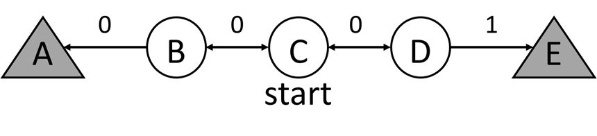
(a)

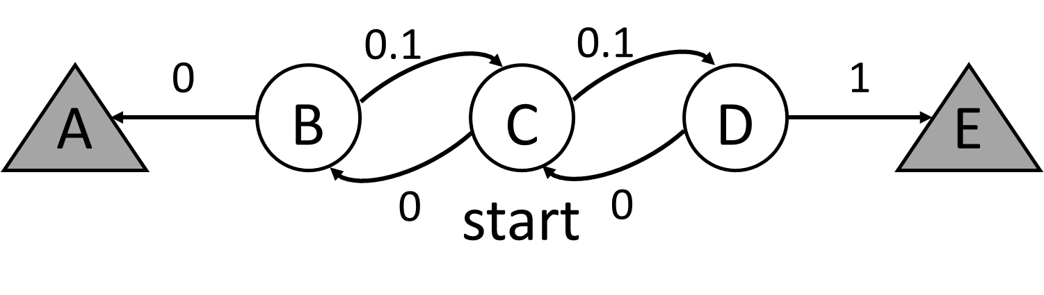
(b)

Figure 1: Random Walk example [16], where (a) describes how to receive $R^{T}$ and (b) illustrates how to acquire $R^{A}$.

In this section, we showcase the efficiency and simplicity of TA-Explore through an examination of a Random Walk example [16], a Markov reward process (i.e., an MDP without actions), allowing us to elucidate the core concepts of TA-Explore in an intuitive manner. Figure 1 depicts the Random Walk environment comprising 5 states. It encompasses two terminal states, denoted as A and E, alongside three non-terminal states, labeled as B, C, and D. If the agent reaches either terminal state, the episode concludes. In all episodes, the agent initiates from state C. Subsequently, at each time step, the agent moves either to the left or right with an equal probability. The agent receives a reward of zero for every transition, except when it reaches state E on the right, where it garners a reward of $+1$. The discount factor is set to $\gamma=1$, indicating an undiscounted MDP. Extending this problem to incorporate additional states is straightforward. We simply arrange all the states in a linear fashion, akin to Figure 1 but with a greater number of states. We will explore random walks with 5, 11, and 33 states.

Due to a lack of action here, the agent’s main goal is to acquire state values through experience. Initial value learning is slow and necessitates a substantial number of samples. This is because, initially, the agent only receives immediate feedback (a non-zero reward) when it reaches the terminal state on the right. However, we can expedite learning by assigning simpler tasks to the agent that offer more frequent immediate feedback. For instance, in Figure 1b, we introduce an assistant reward, $R^{A}$, which provides a reward of 0.1 each time the agent moves to the right, except when it reaches the right terminal state, at which point we award 1. It is evident that learning this auxiliary goal is swifter because the agent receives more frequent reward feedback to update its value function. Additionally, as depicted in Figure 2a, a straightforward yet intelligent approach for determining the $\beta(e)$ function might be $\beta(e)=\beta(0)\lambda^{e}$, where $\beta(0)=1$, and $\lambda\in\{0.8,0.9,0.95\}$. The agent could initially begin learning goal $A$ but will quickly shift its focus to mastering goal $M$.

To assess the performance of our proposed method, we opted for a basic value-based algorithm, specifically the temporal-difference learning method (TD(0)) [17] with a constant step size of 0.1, despite the compatibility of TA-Explore with various RL algorithms. This choice is due to Random Walk’s nature as an MRP problem with a discrete state space. In this instance, transfer learning occurs through value transfer, where the value functions derived for each task serve as the initial values for the subsequent task. Our results are an average of 100 test runs, with each execution initializing the state-value functions for all states to zero. The performance measurement hinges on the root mean square (RMS) error between the learned value function and the true value function corresponding to $M$ and $R^{T}$.

Here’s the compressed text:

In Figure 2b, learning $A$ initially yields positive results, with the agent also unintentionally learning $M$ by episode 38, resulting in a reduction in RMS error. However, as the agent prioritizes learning goal $A$, the error increases, reflecting the divergence in the value functions of the two goals; learning $A$ outpaces learning $M$ (refer to Only $R^{T}$ in Figure 2b). Therefore, starting with goal $A$ and subsequently transitioning to goal $M$ before overfitting can maximize prior knowledge utilization. This approach accelerates learning $M$. Specifically, with $\lambda=0.95$, TA-Explore achieves twice faster convergence on goal $M$.

In Figure 2c, even with 11 states, $\lambda=0.95$ remains an effective choice. The critical insight is that as the state count rises, our proposed method’s superiority becomes evident. More states decrease the likelihood of initially reaching the far-right state, slowing down baseline convergence, which heavily relies on state numbers. Conversely, our method maintains a $50\%$ chance of receiving rewards from the first step. In Figure 2d, we consider 33 states where the baseline fails to converge, while TA-Explore succeeds. Notably, $\lambda=0.95$ ceases to be an appropriate choice. As the number of states grows, disparities in true state-value functions emerge, even though the two goals initially align. Spending too much time on auxiliary goal learning hampers the agent’s access to valuable prior information and can lead to extended main goal learning, necessitating time to forget undesirable experiences. Therefore, the agent should transition to main goal learning more quickly, albeit not hastily, as illustrated in Figure 2d with $\lambda=0.9$, resulting in more than double the speed of convergence.

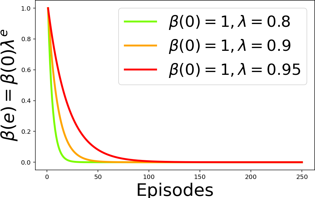
(a) $\beta(e)$

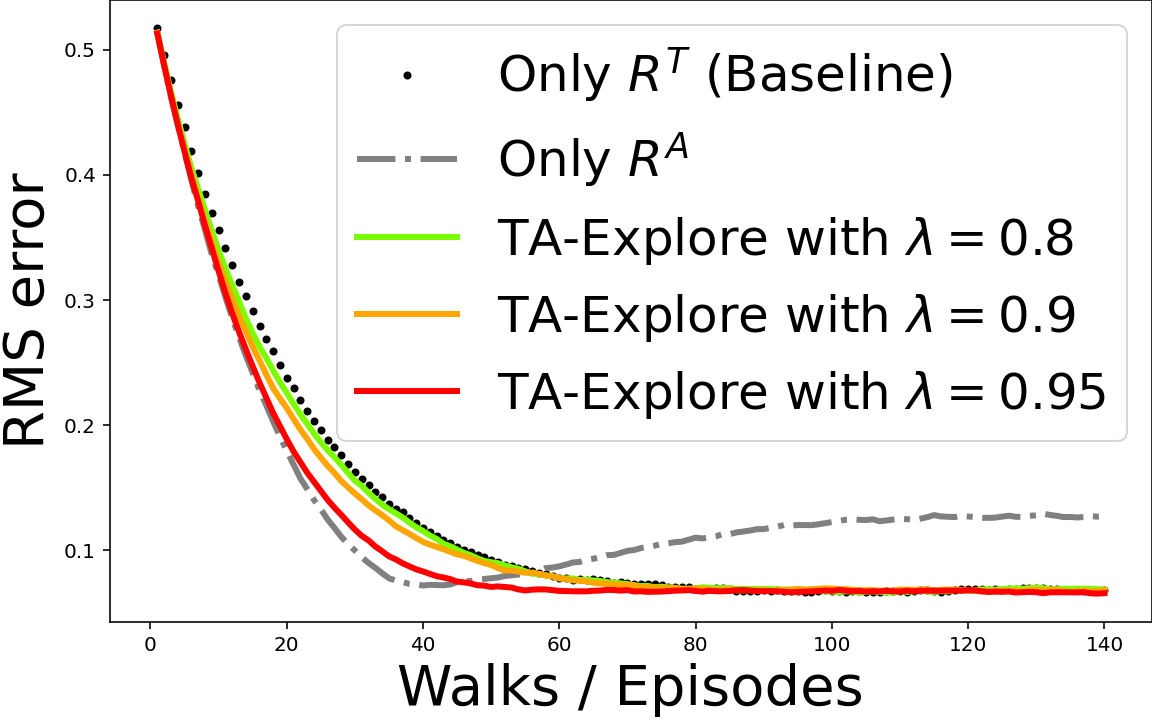
(b) 5 states

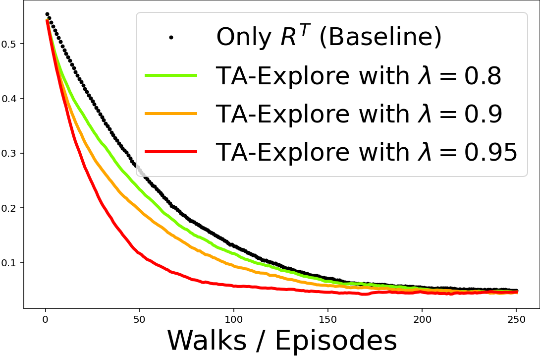
(c) 11 states

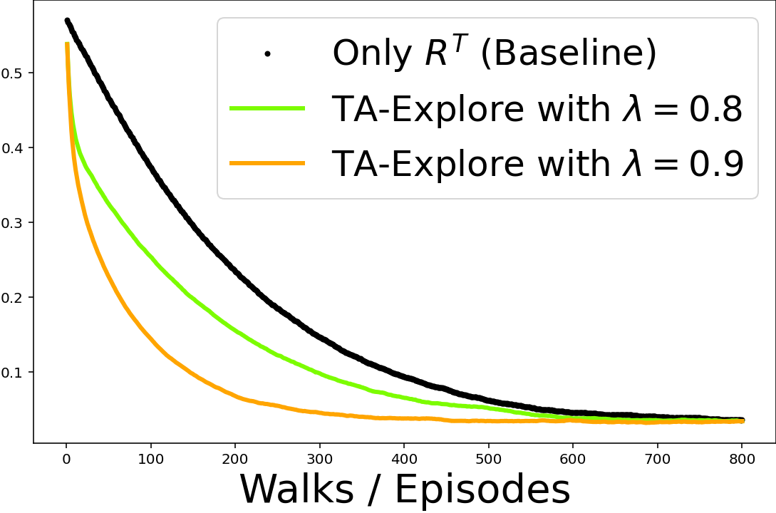
(d) 33 states

Figure 2: (a) The behaviour of the $\beta(e)$ function considered for Random Walk example, with different $\lambda$ values. (b-d) The main goal learning curves in the Random Walk example for different $\lambda$ values and the different number of states. The undrawn curves in (c) and (d) have diverged and have been omitted to show the rest of the results in more detail.

IV Experiment on Control Problems

We illustrate the promise of the TA-Explore framework on two optimal control problems with constraints. We consider a dynamical system governed by the difference equation $s_{t+1}=g_{t}(s_{t},a_{t},e_{t})$, where $s_{t}$ is the state of the system, $a_{t}$ is the control action, and $e_{t}$ is a random disturbance; $g_{t}$ is the rule that maps the current state, control action, and disturbance at time $t$ to a new state. The goal of the agent is to find the actions that optimize the accumulated immediate rewards $f_{t}(s_{t},a_{t})$. Often there are also constraints on the states. Thus, the agent should not only optimize its rewards, but it should also ensure the feasibility of the states. This could be, for example, to ensure the safety of the system operations. Mathematically, such problems are formulated as follows:

$$\begin{split}\text{maximize}&\sum_{t=0}^{H}\gamma^{t}f_{t}(s_{t},a_{t})\\ \text{subject to }&s_{t+1}=g_{t}(s_{t},a_{t},e_{t}),\text{and }\\ &s_{\min}\leqslant s_{t}\leqslant s_{\max}.\end{split}$$

The constraints on state variable $s_{t}$ pose challenges for optimal control, resembling real-world issues. Even with known linear dynamics $g_{t}(s_{t},a_{t},e_{t})$ and quadratic rewards, traditional LQ-regulators cannot handle it due to the state constraint [18]. Furthermore, the problem is exacerbated by the typical lack of knowledge about the system’s dynamics [19]. In such cases, learning-based methods, such as RL, are often the only viable solutions.

In RL, constraints are typically incorporated into the reward as the main goal $M$ via a penalty for violations. This means the RL agent must simultaneously learn to satisfy constraints while optimizing rewards. Learning to satisfy constraints is relatively easier because the agent has more action choices, facilitating constraint satisfaction. Hence, it makes sense to use constraint satisfaction as the auxiliary goal $A$ in our framework. We achieve this by employing a negative assistant reward $R^{A}$. As $R^{A}$ is part of the target reward $R^{T}$, there is a strong alignment between them. Consequently, the $\beta(e)$ function can be selected more easily. Our choice is a descending linear function, starting at $\beta(0)$ and reaching zero at $e=E$. This results in a sequence of $E$ MDPs, each solved over one episode.

IV-A Optimal Temperature Control with Constraint - Linear Dynamics

Consider a data center cooling where three heat sources are coupled to their own cooling devices. Each component of the state $s$ is the internal temperature of one heat source, which should be maintained in the range of -2 to 2 (i.e., we have constraints on states such that $-2\leqslant s_{t}\leqslant 2$). Under constant load, the sources heat up and radiate heat into the surrounding environment. The voltage of each cooler is known as $a$, and the objective is to minimize it while satisfying the constraint. It can be approximated by the linear dynamical system $s_{t+1}=As_{t}+Ba_{t}+e_{t}$ where,

$$A=\begin{bmatrix}1.01&0.01&0\\ 0.01&1.01&0.01\\ 0&0.01&1.01\end{bmatrix}~{}~{}~{}~{},~{}~{}~{}~{}B=I,$$

and where $e_{t}$ is a noise with zero mean with covariance $10^{-4}I$. The voltage of each cooler is the action and the goal is to minimize the power (i.e., $\omega||a||^{2}$) while satisfying the constraint [19]. To put it in our framework, we define the target reward $R^{T}$ and the assistant reward $R^{A}$ as follows:

$$\begin{split}&R^{T}=\begin{cases}-\omega\|a\|^{2}&\text{if constraint is satisfied}\\ -\omega\|a\|^{2}-100&\text{otherwise}\end{cases}\\ &R^{A}=\begin{cases}0&\hskip 36.98866pt\text{if constraint is satisfied}\\ -100&\hskip 36.98866pt\text{otherwise}\end{cases}\end{split}$$ (3)

where $\omega$ is the weight of the first term; its impact will be examined later.

The time horizon is 100 steps, and there are 8000 training episodes. To increase the challenge, states can have any initial value following a standard normal distribution. Episodes do not end if the constraint is not satisfied (training continues for 100 time steps in each episode). For $\beta(e)$, we set $E=4000$ and $\beta(0)=1$, so the objective function equals the main goal $M$ after 4,000 episodes.

To train the agent, we employ PPO, a deep-RL approach, due to its success as a policy-based algorithm [20]. PPO is known for its efficiency, presenting a challenge for improvement. In our setup, we update actor and critic models with mini-batches of 512 samples, using 10 training epochs and the Adam optimizer (LR = 0.00025). We set discount and lambda factors at 0.99 and 0.9, respectively. Both actor and critic models consist of three layers with ReLU activation, with unit sizes of 512, 256, and 64. Actor and critic output layers have 3 and 1 neurons, respectively, utilizing tanh and identity activation functions. In addition to the original PPO, we compare our performance against four state-of-the-art algorithms: A2C [21], DDPG [22], SAC [23], and TD3 [24].

In this example, transfer learning is achieved via policy transfer using episode-obtained weights for each task as initial neural network weights for the next task. Figure 3 displays TA-Explore framework performance. Our framework maintains the same hyperparameters as PPO, streamlining its applicability across various algorithms without requiring further tuning. Other algorithm implementations are based on the Stable Baselines3 repository [25]. Performance evaluation involves plotting the average reward $R^{T}$, a pertinent metric as the primary focus of the agent is mastering the main goal $M$; the auxiliary goal $A$ serves solely as a learning facilitator. Consequently, acquiring proficiency in the auxiliary goal $A$ has no intrinsic importance, unless it expedites knowledge transfer for faster convergence.

In Figure 3a, TA-Explore converges twice as fast because of rapid learning of assistant reward $R^{A}$ in early episodes. Other algorithms exhibit slower convergence due to the agent’s struggle in discerning complex rewards, making it challenging to differentiate constraint violations from deviations from the main goal. Prioritizing the initial term of $R^{T}$ sacrifices more information from $R^{A}$, diminishing alignment between them, thus heightening the challenge. Nonetheless, as depicted in Figures 3b and 3c, TA-Explore converges nearly as swiftly. In contrast, the baselines yield unsatisfactory results, often failing to converge even after 8,000 episodes. Thus, it is evident that for more intricate problems, our convergence outpaces the baselines. It is worth noting that, while we have demonstrated the significance of learning constraints and gradually incorporating the primary problem, further enhancement can be achieved through skillful formulation of auxiliary goals informed by domain knowledge.

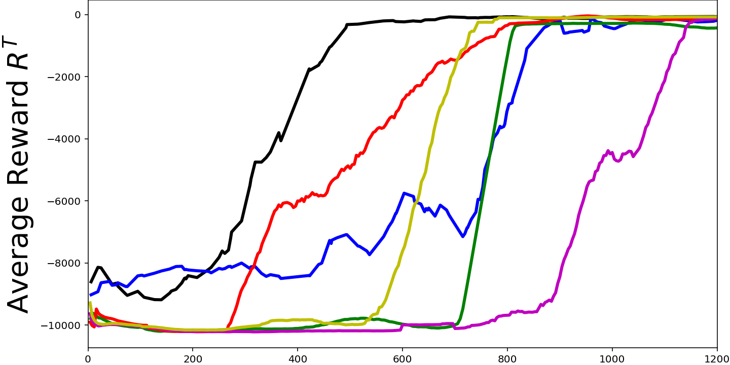
(a)

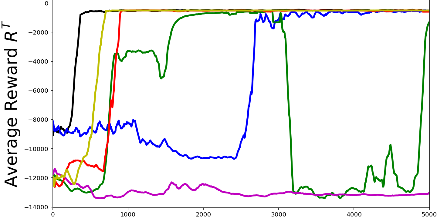
(b)

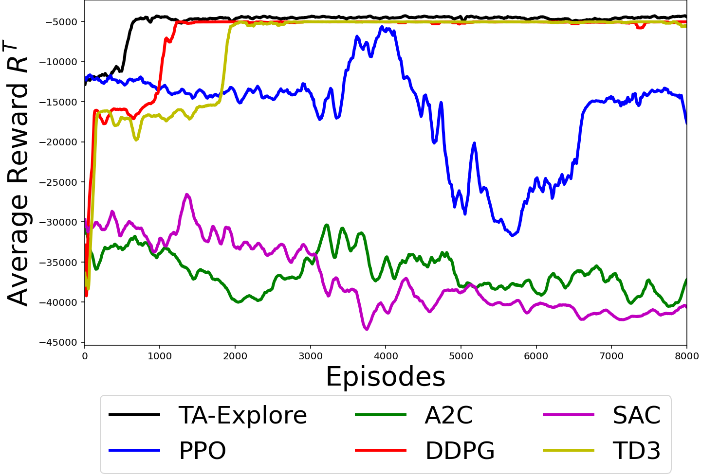
(c)

Figure 3: Average performance on optimal temperate control problem for different weighting values to the control objective (i.e., (a) $1\|a\|^{2}$, (b) $10\|a\|^{2}$, (c) $100\|a\|^{2}$). To have a clear illustration, 50 episodes moving average reward are plotted.

IV-B Coupled Four Tank MIMO System - Nonlinear Dynamics

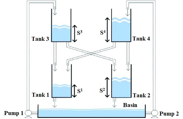
Figure 4: Coupled four tank MIMO system [26] .

We also study the performance on a coupled four-water tank system with nonlinear dynamics [26]. Figure 4 illustrates how this system is comprised of a liquid basin, two pumps, and four tanks with the same area with orifices. The dynamics of the systems are given by:

$$\begin{cases}s_{t+1}^{1}=&-c_{1}\sqrt{s_{t}^{1}}+c_{2}\sqrt{s_{t}^{3}}+c_{3}\sqrt{s_{t}^{4}}\\ s_{t+1}^{2}=&-c_{4}\sqrt{s_{t}^{2}}+c_{5}\sqrt{s_{t}^{3}}+c_{6}\sqrt{s_{t}^{4}}\\ s_{t+1}^{3}=&-c_{7}\sqrt{s_{t}^{3}}+c_{8}a_{t}^{1}\\ s_{t+1}^{4}=&-c_{9}\sqrt{s_{t}^{4}}+c_{10}a_{t}^{2}\end{cases}$$

where $c_{1},...,c_{10}$ are model parameters that are set as in [26]. The actions are $a^{1}$ and $a^{2}$, which indicate the voltages applied, respectively, to Pump 1 and Pump 2, which are bounded between 0 and 12Volts. The states $s^{1}$, $s^{2}$, $s^{3}$, and $s^{4}$ indicate the liquid levels in the four tanks. They should always be greater than 3cm and less than 30cm (i.e., we have constraints both on states and actions such that $3\leqslant s_{t}\leqslant 30$, $0\leqslant a_{t}\leqslant 12$).

The problem can be integrated into our proposed framework using the same rewards from Equation 3 ($\omega=1$). We employ TA-Explore with $\beta(e)=[(E-e)\beta(0)/E]_{+}$, where $\beta(0)=0.5$ and $E=3000$. Initial state values are uniformly distributed between 3 and 30. Episodes are terminated if constraints are not met. All other settings remain consistent with Section IV-A, with training requiring 30,000 episodes due to its complexity. In this experiment, we use PPO with settings identical to those in Section IV-A, except the number of actor model output neurons is 2. Ensuring action feasibility is straightforward because the actor model’s output, governed by the tanh activation function, scales between 0 and 12.

Figure 5 demonstrates the performance contrast between our proposed approach and baseline methods. Notably, TA-Explore consistently converges to the target reward over $30\%$ faster than PPO, regardless of problem complexity or suboptimal $\beta(e)$ choices. This remarkable convergence stands in contrast to the other baselines, which struggle to reach convergence. The choice of $\beta(0)=0.5$ signifies that from the very first episode, our method prioritizes minimizing voltage while respecting constraints, albeit with half the weight compared to the target reward $R^{T}$.

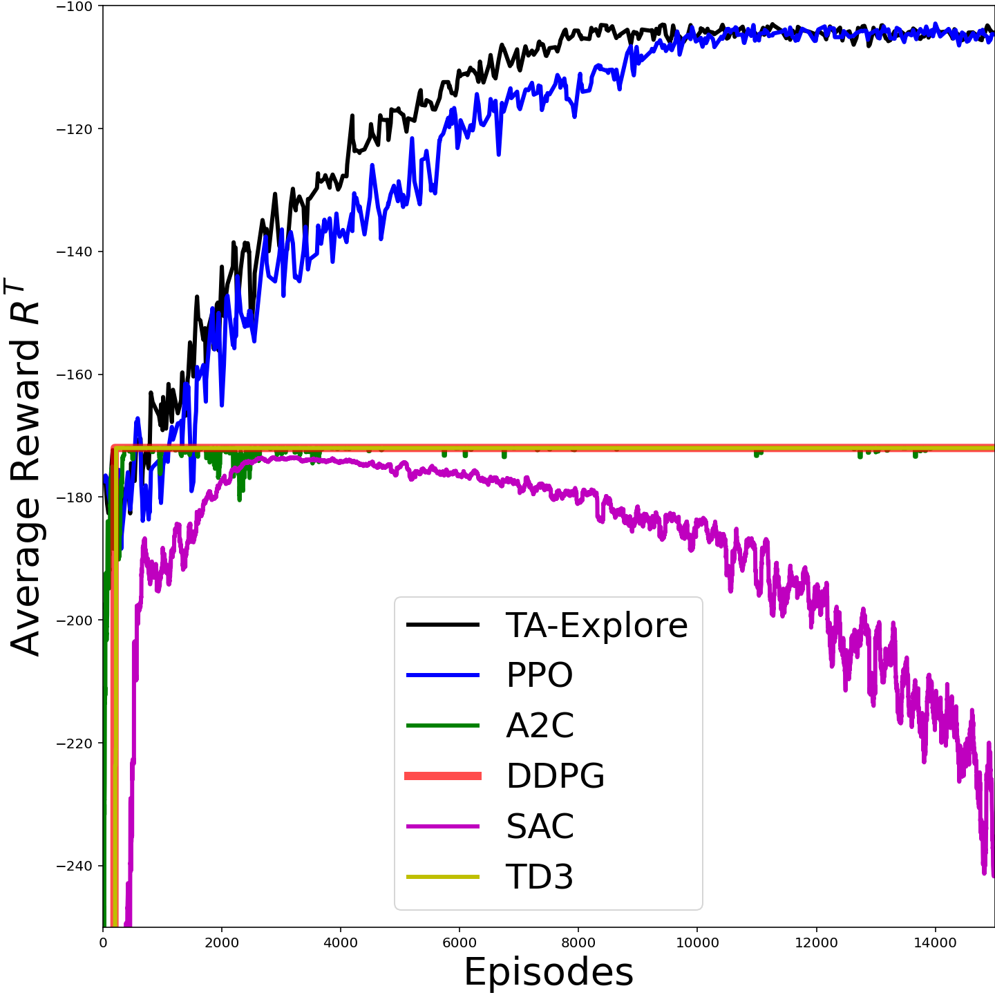
Figure 5: Performance on coupled four tank MIMO system. To have a clear illustration, 50 episodes moving average reward are plotted.

V Related Work

To the best of our knowledge, this paper stands out from the rest of the studies because first, we use a sequence of auxiliary goals (i.e., MDPs) by defining only one assistant reward (not many and not following from a particular distribution) and an annealing function. Second, we learn each auxiliary task only one iteration (without necessarily having $\epsilon$-accuracy with $\delta$ probability assumption). And third, our proposed method supports policy and value transfers, which leads our approach to combine with any type of RL-based algorithm to improve sample efficiency. However, the scope of related work can be broadened to include other efforts to help the agent learn its main task more efficiently. It should be noted that due to the strong assumptions of other studies stated in this section, it is not possible to use them in our experiments. That is why we have to limit the comparison of our method with the original algorithms.

Improving the exploration process of an RL agent has been well-studied in the literature. Many previous efforts are based on the hypothesis that if we can visit as many states as possible with high probability, then the agent’s learning will be more successful and sample efficient. In other words, further exploration is in line with achieving the main goal of the RL agent. There are two fundamental questions that emerge in this setting. In the absence of rewards, what are the agents supposed to look for? And at what point should the agent stop exploring and start acting greedily? Research that seeks to answer these questions can be divided into two general categories. Firstly, there are single-environment approaches, which include intrinsic motivation with visitation counts [13, 14], optimism [27, 28], curiosity [29, 30, 31] , and reward shaping [32]. Secondly, there are multi-environment approaches that incrementally learn a task across environments, for example, through transfer learning [33, 34, 35, 36, 37], continual learning [38], meta-learning [39], and curriculum learning [40, 41]. We discuss these approaches below and contrast them to our contributions.

Single-environment: The notion of intrinsic rewards for exploration originated with Schmidhuber [42], who proposed encouraging exploration by visiting unpredictable states. In recent years, researchers in RL have extensively studied auxiliary rewards to compensate for the lack of external rewards. Many intrinsic rewards have been proposed, including bonuses based on visitation counts and prediction errors [13, 14]. For instance, a dynamic model can be learned to predict the next state [29, 30]. Here, the agent is incentivized to explore unpredictable states by granting a bonus proportional to its prediction error. Another idea, by Schultheis et al. [31], is to maximize extrinsic rewards by meta-gradient to learn intrinsic rewards. Also, potential-based reward shaping to encourage agents to explore more has been studied as a way of increasing the learning speed [32].

These methods of exploration are often called agent-centric since they are based on updating the agent’s belief, e.g., through the forward model error. In this sense, these works fall into the same category as ours; both rely on the hypothesis that exploration at the same time with exploitation by agents can be sufficient to achieve a (sub-) optimal policy. Another common assumption is that in all the papers following this method, the main goal and, consequently, the target award, i.e., the extrinsic reward is clear, and we have knowledge about it. The main difference between our work and others is that their purpose in the first place is only to explore as much as possible, and they are based on the assumption that by exploring more, the agent can learn an optimal policy. In contrast, we do not have such an assumption, and we do not seek to visit the states as much as possible. Instead, we focus only on intelligent and auxiliary exploration, which is resulted from transferred knowledge gained on intermediate partially solved tasks, which is in line with the main goal and accelerates the learning of the main task, not a complete acquaintance of the environment.

Multi-environment: The second set of papers reviewed followed the idea of incrementally learning tasks that have long been known in machine learning [43]. In RL, although recent methods have mostly focused on policy and feature transfer, some have studied exploration transfer [34]. In policy transfer, behaviors are transferred to a new agent (student) by a pre-trained agent (teacher). The student is trained to minimize the KullbackLeibler divergence to the teacher using policy distillation, for example, [44]. Other methods re-use policies from source tasks directly to create a student policy [45, 46]. On the other hand, a pre-learned state representation used in feature transfer encourages the agent to explore when it is presented with tasks [47]. In exploration transfer, in a task-agnostic and environment-centric scenario, the agent is first attempted by defining an intrinsic reward to visit the states as more as possible especially interesting states in multiple environments, instead of learning the main task, and then this prior knowledge is transferred as a bias to the main environment in which the main task is to be trained [34]. Studies on continual RL seek to determine how learning one or more tasks can accelerate learning of other tasks, as well as avoid ruinous forgetting [38]. Meta RL and curriculum learning, on the other hand, focus on exploiting underlying similarities between tasks to speed up the learning process of new tasks [39, 40, 41]. Many studies have been done under the Lifelong RL framework, where the tasks change following a specific distribution [35, 36, 37]. In [36, 37], by spending a lot of computational costs, knowledge transfer is done through transferring initializers. Most are only compatible with ($\epsilon$, $\delta$)-PAC algorithms [35, 36, 37, 15]

In the mentioned incrementally learning task methods, it is assumed that there are several tasks/environments that, with the help of the experience gained on one or multiple tasks/environments, we seek to accelerate the learning of the same task in the new environment or the new task in the same environment. As a result, the most important hypothesis is that tasks/environments are very similar to each other, which is not always consistent with reality and deprives us of the possibility of using these methods on any task and any environment. On the contrary, our proposed framework does not need to have several similar environments/tasks. In particular, by defining only one assistant reward along with a decreasing function, we successfully represent a large number of MDPs, which essentially does not require the assumption of switching tasks over a particular distribution. Therefore, it can be used for any environment and any task. Another point is that in transfer learning, the learning process consists of two phases pre-training and the end-training phase, which are isolated from each other. More specifically, it is assumed that the learning on the previous tasks has been done thoroughly and with good accuracy. In our proposed framework, however, we are smoothly and consistently shifting between the auxiliary goals and the main goal. Not only do we not assume any tasks are already learned, but we also do not need to learn them completely and accurately, i.e., we only have one iteration of training per auxiliary task. In the other studies, like [35], which identify the closest task for knowledge transfer, there is a lot of computational cost and limit on the learning transfer method and the algorithms that can be combined with their methods. But our approach does not add computational complexity. Also, it can transfer knowledge through both value and policy transfer and is compatible with any algorithm. Note that we have an integrated learning process so that when considering the acceleration of convergence, we do not neglect to consider the time required to learn the auxiliary goals. The last issue is related to [34], where the authors try to explore as much as possible in the pre-training stage. On the contrary, we do not suppose such a hypothesis in our work. As a result, we only focus on defining auxiliary goals for faster learning of the task.

VI Conclusion and Future Work

Sample inefficiency is a critical weakness of current developments in RL. RL algorithms must become more efficient if they are to achieve their full potential in many real-world applications. In this paper, we introduce a new framework TA-Explore for smart exploration. The main idea is to use simpler assistant tasks that are aligned with the main task that gradually progress toward the main difficult task. Thus helping the agent in finding a more efficient learning trajectory. The TA-Explore framework is extremely flexible; it can be applied to any RL task, any type of environment. In addition, any type of RL algorithm can be used as its backbone. We conducted comprehensive experiments on a wide range of tasks with different difficulties, with different RL algorithms -both value-based methods and policy-based methods and both tabular methods and deep-RL methods. The results show the excellent performance of the proposed method in increasing the convergence speed. Moreover, TA-Explore has no additional computational cost and complexity. Therefore, our proposed framework, which owes its superiority to the definition of the teacher-assisted goal, can impact the field of RL and make researchers think about a better definition of the reward, relaxing limiting assumptions, and no need to complete learning of the prior tasks before the transfer learning process. Proving the sample complexity improvement in such a setting is potentially future work. Also, for future work, adding a self-tuning feature to the $\beta$ function can go a long way in overcoming the only current limitation of the proposed method, which is to select the $\beta$ function experimentally. On the other hand, examining its performance in multi-agent environments under the partially observable Markov decision process (POMDP) assumption, which has higher complexity and suffers from slow learning of the objective function, can be considered a valuable task.

References

- [1] V. Mnih, K. Kavukcuoglu, D. Silver, A. A. Rusu, J. Veness, M. G. Bellemare, A. Graves, M. Riedmiller, A. K. Fidjeland, G. Ostrovski et al., “Human-level control through deep reinforcement learning,” nature, vol. 518, no. 7540, pp. 529–533, 2015.
- [2] D. Silver, J. Schrittwieser, K. Simonyan, I. Antonoglou, A. Huang, A. Guez, T. Hubert, L. Baker, M. Lai, A. Bolton et al., “Mastering the game of go without human knowledge,” nature, vol. 550, no. 7676, pp. 354–359, 2017.
- [3] T. L. Meng and M. Khushi, “Reinforcement learning in financial markets,” Data, vol. 4, no. 3, p. 110, 2019.
- [4] J. Kober, J. A. Bagnell, and J. Peters, “Reinforcement learning in robotics: A survey,” The International Journal of Robotics Research, vol. 32, no. 11, pp. 1238–1274, 2013.
- [5] R. Sutton, A. Barto, and R. Williams, “Reinforcement learning is direct adaptive optimal control,” IEEE Control Systems Magazine, vol. 12, no. 2, pp. 19–22, 1992.
- [6] S. Shalev-Shwartz, S. Shammah, and A. Shashua, “Safe, multi-agent, reinforcement learning for autonomous driving,” arXiv preprint arXiv:1610.03295, 2016.
- [7] C. J. C. H. Watkins and P. Dayan, “Q -learning,” Mach. Learn., vol. 8, no. 3–4, p. 279–292, may 1992.
- [8] Y. Yu, “Towards sample efficient reinforcement learning.” in IJCAI, 2018, pp. 5739–5743.
- [9] F. Sung, L. Zhang, T. Xiang, T. Hospedales, and Y. Yang, “Learning to learn: Meta-critic networks for sample efficient learning,” 2017.
- [10] M. Turchetta, A. Kolobov, S. Shah, A. Krause, and A. Agarwal, “Safe reinforcement learning via curriculum induction,” in Advances in Neural Information Processing Systems, H. Larochelle, M. Ranzato, R. Hadsell, M. F. Balcan, and H. Lin, Eds., vol. 33. Curran Associates, Inc., 2020, pp. 12 151–12 162.
- [11] G. Anderson, A. Verma, I. Dillig, and S. Chaudhuri, “Neurosymbolic reinforcement learning with formally verified exploration,” in Advances in Neural Information Processing Systems, H. Larochelle, M. Ranzato, R. Hadsell, M. F. Balcan, and H. Lin, Eds., vol. 33. Curran Associates, Inc., 2020, pp. 6172–6183.
- [12] J. Gottlieb, P.-Y. Oudeyer, M. Lopes, and A. Baranes, “Information-seeking, curiosity, and attention: computational and neural mechanisms,” Trends in Cognitive Sciences, vol. 17, no. 11, pp. 585–593, 2013.
- [13] M. Bellemare, S. Srinivasan, G. Ostrovski, T. Schaul, D. Saxton, and R. Munos, “Unifying count-based exploration and intrinsic motivation,” in Advances in Neural Information Processing Systems, D. Lee, M. Sugiyama, U. Luxburg, I. Guyon, and R. Garnett, Eds., vol. 29. Curran Associates, Inc., 2016.
- [14] A. L. Strehl and M. L. Littman, “An analysis of model-based interval estimation for markov decision processes,” Journal of Computer and System Sciences, vol. 74, no. 8, pp. 1309–1331, 2008, learning Theory 2005.
- [15] A. L. Strehl, L. Li, and M. L. Littman, “Reinforcement learning in finite mdps: Pac analysis.” Journal of Machine Learning Research, vol. 10, no. 11, 2009.
- [16] R. S. Sutton and A. G. Barto, Reinforcement learning: An introduction. MIT press, 2018.
- [17] G. Tesauro et al., “Temporal difference learning and td-gammon,” Communications of the ACM, vol. 38, no. 3, pp. 58–68, 1995.
- [18] K. J. Åström and R. M. Murray, “Feedback systems,” An Introduction for Scientists and Engineers, Karl Johan Åström and Richard M. Murray, 2007.
- [19] B. Recht, “A tour of reinforcement learning: The view from continuous control,” Annual Review of Control, Robotics, and Autonomous Systems, vol. 2, pp. 253–279, 2019.
- [20] J. Schulman, F. Wolski, P. Dhariwal, A. Radford, and O. Klimov, “Proximal policy optimization algorithms,” arXiv preprint arXiv:1707.06347, 2017.
- [21] V. Mnih, A. P. Badia, M. Mirza, A. Graves, T. Lillicrap, T. Harley, D. Silver, and K. Kavukcuoglu, “Asynchronous methods for deep reinforcement learning,” in International conference on machine learning. PMLR, 2016, pp. 1928–1937.
- [22] T. P. Lillicrap, J. J. Hunt, A. Pritzel, N. Heess, T. Erez, Y. Tassa, D. Silver, and D. Wierstra, “Continuous control with deep reinforcement learning,” arXiv preprint arXiv:1509.02971, 2015.
- [23] T. Haarnoja, A. Zhou, P. Abbeel, and S. Levine, “Soft actor-critic: Off-policy maximum entropy deep reinforcement learning with a stochastic actor,” in International conference on machine learning. PMLR, 2018, pp. 1861–1870.
- [24] S. Fujimoto, H. Hoof, and D. Meger, “Addressing function approximation error in actor-critic methods,” in International conference on machine learning. PMLR, 2018, pp. 1587–1596.
- [25] A. Raffin, A. Hill, A. Gleave, A. Kanervisto, M. Ernestus, and N. Dormann, “Stable-baselines3: Reliable reinforcement learning implementations,” Journal of Machine Learning Research, vol. 22, no. 268, pp. 1–8, 2021. [Online]. Available: http://jmlr.org/papers/v22/20-1364.html
- [26] H. Gouta, S. Hadj Saïd, N. Barhoumi, and F. M’Sahli, “Generalized predictive control for a coupled four tank mimo system using a continuous-discrete time observer,” ISA Transactions, vol. 67, pp. 280–292, 2017.
- [27] P. Auer and R. Ortner, “Logarithmic online regret bounds for undiscounted reinforcement learning,” in Advances in Neural Information Processing Systems, B. Schölkopf, J. Platt, and T. Hoffman, Eds., vol. 19. MIT Press, 2007.
- [28] P. Auer, T. Jaksch, and R. Ortner, “Near-optimal regret bounds for reinforcement learning,” in Advances in Neural Information Processing Systems, D. Koller, D. Schuurmans, Y. Bengio, and L. Bottou, Eds., vol. 21. Curran Associates, Inc., 2009.
- [29] R. Houthooft, X. Chen, X. Chen, Y. Duan, J. Schulman, F. De Turck, and P. Abbeel, “Vime: Variational information maximizing exploration,” in Advances in Neural Information Processing Systems, D. Lee, M. Sugiyama, U. Luxburg, I. Guyon, and R. Garnett, Eds., vol. 29. Curran Associates, Inc., 2016.
- [30] D. Pathak, P. Agrawal, A. A. Efros, and T. Darrell, “Curiosity-driven exploration by self-supervised prediction,” in Proceedings of the 34th International Conference on Machine Learning, ser. Proceedings of Machine Learning Research, D. Precup and Y. W. Teh, Eds., vol. 70. PMLR, 06–11 Aug 2017, pp. 2778–2787.
- [31] M. Schultheis, B. Belousov, H. Abdulsamad, and J. Peters, “Receding horizon curiosity,” in Proceedings of the Conference on Robot Learning, ser. Proceedings of Machine Learning Research, L. P. Kaelbling, D. Kragic, and K. Sugiura, Eds., vol. 100. PMLR, 30 Oct–01 Nov 2020, pp. 1278–1288.
- [32] M. Dann, F. Zambetta, and J. Thangarajah, “Deriving subgoals autonomously to accelerate learning in sparse reward domains,” Proceedings of the AAAI Conference on Artificial Intelligence, vol. 33, no. 01, pp. 881–889, Jul. 2019.
- [33] K. Weiss, T. M. Khoshgoftaar, and D. Wang, “A survey of transfer learning,” Journal of Big data, vol. 3, no. 1, pp. 1–40, 2016.
- [34] S. Parisi, V. Dean, D. Pathak, and A. Gupta, “Interesting object, curious agent: Learning task-agnostic exploration,” Advances in Neural Information Processing Systems, vol. 34, 2021.
- [35] A. Tirinzoni, R. Poiani, and M. Restelli, “Sequential transfer in reinforcement learning with a generative model,” in International Conference on Machine Learning. PMLR, 2020, pp. 9481–9492.
- [36] D. Abel, Y. Jinnai, S. Y. Guo, G. Konidaris, and M. Littman, “Policy and value transfer in lifelong reinforcement learning,” in International Conference on Machine Learning. PMLR, 2018, pp. 20–29.
- [37] E. Lecarpentier, D. Abel, K. Asadi, Y. Jinnai, E. Rachelson, and M. L. Littman, “Lipschitz lifelong reinforcement learning,” in Proceedings of the AAAI Conference on Artificial Intelligence, vol. 35, 2021, pp. 8270–8278.
- [38] J. Kirkpatrick, R. Pascanu, N. Rabinowitz, J. Veness, G. Desjardins, A. A. Rusu, K. Milan, J. Quan, T. Ramalho, A. Grabska-Barwinska, D. Hassabis, C. Clopath, D. Kumaran, and R. Hadsell, “Overcoming catastrophic forgetting in neural networks,” Proceedings of the National Academy of Sciences, vol. 114, no. 13, pp. 3521–3526, 2017.
- [39] C. Finn, P. Abbeel, and S. Levine, “Model-agnostic meta-learning for fast adaptation of deep networks,” in International conference on machine learning. PMLR, 2017, pp. 1126–1135.
- [40] S. Narvekar, B. Peng, M. Leonetti, J. Sinapov, M. E. Taylor, and P. Stone, “Curriculum learning for reinforcement learning domains: A framework and survey,” arXiv preprint arXiv:2003.04960, 2020.
- [41] S. Luo, H. Kasaei, and L. Schomaker, “Accelerating reinforcement learning for reaching using continuous curriculum learning,” in 2020 International Joint Conference on Neural Networks (IJCNN). IEEE, 2020, pp. 1–8.
- [42] J. Schmidhuber, “A possibility for implementing curiosity and boredom in model-building neural controllers,” in Proc. of the international conference on simulation of adaptive behavior: From animals to animats, 1991, pp. 222–227.
- [43] M. B. Ring et al., “Continual learning in reinforcement environments,” PhD thesis, University of Texas at Austin, 1994.
- [44] A. A. Rusu, S. G. Colmenarejo, Çaglar Gülçehre, G. Desjardins, J. Kirkpatrick, R. Pascanu, V. Mnih, K. Kavukcuoglu, and R. Hadsell, “Policy distillation,” in ICLR (Poster), 2016.
- [45] F. Fernández and M. Veloso, “Probabilistic policy reuse in a reinforcement learning agent,” in Proceedings of the Fifth International Joint Conference on Autonomous Agents and Multiagent Systems, ser. AAMAS ’06. New York, NY, USA: Association for Computing Machinery, 2006, p. 720–727.
- [46] A. Barreto, W. Dabney, R. Munos, J. J. Hunt, T. Schaul, H. P. van Hasselt, and D. Silver, “Successor features for transfer in reinforcement learning,” in Advances in Neural Information Processing Systems, I. Guyon, U. V. Luxburg, S. Bengio, H. Wallach, R. Fergus, S. Vishwanathan, and R. Garnett, Eds., vol. 30. Curran Associates, Inc., 2017.
- [47] S. Hansen, W. Dabney, A. Barreto, D. Warde-Farley, T. V. de Wiele, and V. Mnih, “Fast task inference with variational intrinsic successor features,” in International Conference on Learning Representations, 2020.