Tau Polarization and Correlated Decays in Neutrino Experiments

Abstract

We present the first fully differential predictions for tau neutrino scattering in the energy region relevant to the DUNE experiment, including all spin correlations and all tau lepton decay channels. The calculation is performed using a generic interface between the neutrino event generator Achilles and the publicly available, general-purpose collider event simulation framework Sherpa.

I Introduction

The tau neutrino is commonly considered to be the least well known elementary particle. The first experimental direct evidence for tau neutrinos was provided about two decades ago by the DONuT experiment Kodama et al. (2001). Major limitations on the dataset came from a small cross section, the large mass of the tau lepton, and the large irreducible backgrounds. As of today, there are still very few positively identified tau neutrino events from collider based sources, with 9 detected by DONuT Kodama et al. (2008), and 10 detected by OPERA Agafonova et al. (2018). The SuperK Li et al. (2018), and IceCube Aartsen et al. (2019); Abbasi et al. (2022) experiments have identified 291 and 1806 tau neutrino candidates from atmospheric and astrophysical sources. New experiments are expected to come online soon, among them DUNE De Gouvêa et al. (2019); Abi et al. (2020) and the IceCube upgrade Ishihara (2021), which will improve the precision on the $\nu_{\mu}\to\nu_{\tau}$ appearance measurement. The forward physics facility Feng et al. (2023) will use the large forward charm production rate at the LHC to perform precision studies with collider neutrinos. Ultra-high energy neutrino telescopes will set limits on $\nu_{\tau}$ self-interactions (which are currently unconstrained Esteban et al. (2021)) and flavor ratios (which are an important observable to constrain new physics Argüelles et al. (2020)). With all of these novel experiments, the tau neutrino dataset is expected to grow quickly in the coming years, creating new opportunities for measurements and searches for physics beyond the standard neutrino paradigm Mammen Abraham et al. (2022).

DUNE is especially important to the tau neutrino program, since it will be the only accelerator based experiment able to collect and accurately reconstruct a sample of oscillated $\nu_{\tau}$ charged current (CC) events, with about 130 $\nu_{\tau}$ CC events per year in CP-optimized neutrino mode, 30 $\bar{\nu}_{\tau}$ events per year in CP-optimized antineutrino mode and about 800 $\nu_{\tau}$ CC events per year in tau-optimized neutrino mode Mammen Abraham et al. (2022). To make the most of these events, accurate theory predictions are required. One key observation to help separate the signal from the irreducible background is the fact that the tau is polarized, leading to correlations in the outgoing pions. However, the produced outgoing tau lepton is not fully polarized for DUNE energies Sobczyk et al. (2019); Hernández et al. (2022). Additionally, the cross section is dominated by quasielastic and resonance scattering. Computational tools that model both the intricate aspects of nuclear physics involved in $\nu$-nucleus interactions and the effects of polarized scattering and decay are vital for experimental success Machado et al. (2020). However, the existing neutrino event generators GENIE Andreopoulos et al. (2010), NuWro Golan et al. (2012), NEUT Hayato and Pickering (2021), and GiBUU Leitner et al. (2006) generate $\nu_{\tau}$ interactions in the same manner as $\nu_{e}$ and $\nu_{\mu}$ events. They then assume that the outgoing $\tau$ is purely left-handed and simulate its decay with the help of TAUOLA Chrzaszcz et al. (2018). We will address this shortcoming by constructing an event generator based on a state-of-the art nuclear physics model, in combination with a general-purpose tau decay simulation including spin correlations between the production and all subsequent decays.

Various theoretical calculations have also addressed nuclear effects on the polarization of the tau in neutrino scattering. However, the previous works either do not include tau decays Sobczyk et al. (2019), or they only include the one-body decay of the tau (i.e. $\tau^{-}\to\nu_{\tau}\pi^{-}$) Hernández et al. (2022). They demonstrate the dependence of the nuclear effects on the polarization and the impact on observables, respectively. Here, we extend these studies to include all possible decay channels of the tau, while maintaining complete polarization information, and we provide a publicly available simulation package to generate fully differential final states. The calculation is performed using Achilles Isaacson et al. (2023) to handle the nuclear physics effects and Sherpa Gleisberg et al. (2004, 2009); Bothmann et al. (2019) to perform the leptonic calculation and the decay of the tau. This interface extends the one developed in Ref. Isaacson et al. (2022), which also allows to perform the calculation in nearly arbitrary new physics models by means of FeynRules Christensen and Duhr (2009); Alloul et al. (2014).

The outline of this paper is as follows. In Sec. II, we review analytic results on the production and decay of the tau, with a focus on the effects of nuclear physics and the high energy limit. The implementation of tau decays within the Sherpa framework and the interface between Achilles and Sherpa is described in Sec. III. Comparisons for purely left-handed and the correct polarization is shown for various monochromatic neutrino beam energies as well as for a realistic tau-optimized DUNE neutrino flux in Sec. IV.

II Polarization in tau lepton production and decay

This section provides a brief overview of the main analytic results on the effect of polarization in $\tau$ decays and production. The collinear limit, which provides both theoretical insight and a useful benchmark for the validation of Monte-Carlo simulations, is discussed in some detail. Furthermore, the dependency of the polarization of the $\tau$ on the hadronic tensor is reviewed.

II.1 Tau Decays in the Collinear Limit

The dominant decay channels of the $\tau$ are into a single pion, leptons, or into a vector meson resonance. In these channels, ignoring the decays of the vector mesons, the distribution of the final state momenta can be determined in the collinear limit (i.e. $p_{\tau}\to\infty$). These results are useful for the validation of more detailed theoretical predictions.

The rate of the $\tau^{\mp}\rightarrow\pi^{\mp}\nu_{\tau}$ decay in the rest frame of the tau is given as Bullock et al. (1993)

$$\frac{1}{\Gamma_{\tau}}\frac{{\rm d}\Gamma_{\pi}}{{\rm d}\cos\theta_{\pi}}=\frac{1}{2}B_{\pi}\left(1\pm P_{\tau}\cos\theta_{\pi}\right)\,,$$ (1)

where $B_{\pi}$ is the branching fraction of $\tau\rightarrow\pi\nu_{\tau}$, $P_{\tau}$ is the polarization of the $\tau$, and $\theta_{\pi}$ is the angle between the pion momentum and the tau spin axis, which coincides with the $\tau$ momentum in the lab frame. For a purely right-(left)-handed $\tau^{-}$, the polarization is $P_{\tau}=+1(-1)$. In terms of the momentum fraction, $x_{\pi}=E_{\pi}/E_{\tau}$, the polar angle is given as

$$\cos\theta_{\pi}=\frac{2x_{\pi}-1-a^{2}}{\beta(1-a^{2})}\,,$$ (2)

where $a=m_{\pi}/m_{\tau}$ and $\beta$ is the velocity of the $\tau$. In the collinear limit, $\beta\rightarrow 1$, and making the approximation $a=0$, one obtains

$$\frac{1}{\Gamma_{\tau}}\frac{{\rm d}\Gamma_{\pi}}{{\rm d}x_{\pi}}=B_{\pi}\left(1\pm P_{\tau}\left(2x_{\pi}-1\right)\right)\,.$$ (3)

In this limit, we obtain the prediction for the differential decay rate shown in Fig. 1.

Additionally, for the case of leptonic decays in the collinear and massless limit ($m_{e}=m_{\mu}=0$) the tau decay to leptons is the same for electrons and muons. The differential decay rate is given by Bullock et al. (1993)

$$\frac{1}{\Gamma_{\tau}}\frac{{\rm d}\Gamma_{\ell}}{{\rm d}x_{\ell}}=\frac{1}{3}B_{\ell}(1-x_{\ell})\left(\left(5+5x_{\ell}-4x_{\ell}^{2}\right)\mp\left(1+x_{\ell}-8x_{\ell}^{2}\right)\right)\,,$$ (4)

where $x_{\ell}=p_{\ell}/p_{\tau}$, and $B_{\ell}$ is the branching ratio into a given lepton. The rate for leptons is shown in Fig. 1.

Similarly, the decays for the vector meson decay modes $\tau\to v\nu_{\tau}$, with $v=\rho$ or $a_{1}$ are calculated in Ref. Bullock et al. (1993) and the results are reproduced here for convenience. The mesons are separated into the transverse and longitudinal components in the calculation, since the decays $\rho\to 2\pi$ and $a_{1}\to 3\pi$ depend on the polarization of the vector mesons. The angular distribution in the rest frame of the tau is given as:

$$\frac{1}{\Gamma_{\tau}}\frac{{\rm d}\Gamma^{T}_{v}}{{\rm d}\cos\theta_{v}} =B_{v}\frac{m_{v}^{2}}{m_{\tau}^{2}+2m_{v}^{2}}\left(1\mp P_{\tau}\cos\theta_{v}\right)\,,$$ (5)

$$\frac{1}{\Gamma_{\tau}}\frac{{\rm d}\Gamma^{L}_{v}}{{\rm d}\cos\theta_{v}} =B_{v}\frac{\frac{1}{2}m_{v}^{2}}{m_{\tau}^{2}+2m_{v}^{2}}\left(1\pm P_{\tau}\cos\theta_{v}\right)\,,$$ (6)

where again $v=\rho$ or $a_{1}$, $B_{v}$ is the branching ratio for $\tau^{\mp}\to v^{\mp}\nu_{\tau}$, and $\theta_{v}$ is the same angle defined in the pion case. It is important to note that for the case of the longitudinal state the polarization dependence is the same as Eq. (1), while for the transverse state the polarization enters with the opposite sign. Therefore, if the polarization of the vector meson is not measured, then Eqs. (5) and (6) need to be averaged. This suppresses the sensitivity to the polarization of the tau by a factor of $(m_{\tau}^{2}-2m_{v}^{2})/(m_{\tau}^{2}+2m_{v}^{2})$, which is about 0.46 for the case of the $\rho$ and approximately 0.02 for the case of the $a_{1}$ meson.

In the case of the vector mesons, care has to be taken when boosting to the lab frame since the polarizations are not summed over. First, a Wigner rotation Martin and Spearman (1970) is used to align the spin axis. The angle of rotation is given in the collinear limit by Bullock et al. (1993)

$$\cos\omega=\frac{1-a^{2}+(1+a^{2})\cos\theta}{1+a^{2}+(1-a^{2})\cos\theta}\,,$$ (7)

where $a=m_{v}/m_{\tau}$. Rewriting in terms of the momentum fraction ($x_{v}=E_{v}/E_{\tau}$), the decay distributions can be expressed as

$$\frac{1}{\Gamma_{\tau}}\frac{{\rm d}\Gamma_{v}}{{\rm d}x_{v}} =B_{v}H_{v}^{\alpha}(x_{v},m_{v}^{2})\,,$$ (8)

where $\alpha=T$ or $L$ and the expressions for $H_{v}^{T,L}$ are given in Eqs. (2.16) and (2.17) of Ref. Bullock et al. (1993) respectively. The results for the decay distribution including the width for a left-handed $\tau^{-}$ decay are shown in Fig. 1. These distributions provide the main analytic benchmark points for tests of our Monte-Carlo implementation.

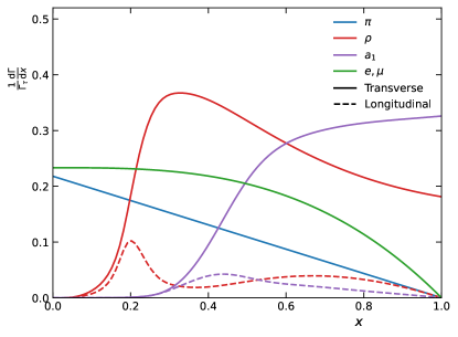
Figure 1: The decay distributions vs the fractional momentum of a given particle to the $\tau$ momentum for a left-handed $\tau^{-}$ in the collinear limit going to single pions (blue), $\rho$ mesons (red), $a_{1}$ mesons (purple), or leptons (green). The vector mesons ($\rho$ and $a_{1}$) can be either transversely polarized (solid lines) or longitudinally polarized (dashed lines). Additionally, the vector mesons are not stable and the effect of their widths are included, which is set to 0.1474 GeV and 0.420 GeV for the $\rho$ and $a_{1}$ respectively.

II.2 Production of the tau lepton

The unpolarized differential cross-section for CC interaction $\nu_{\tau}A\to\tau^{-}X$ can be expressed as the product of a leptonic and hadronic tensor as shown in Ref. Isaacson et al. (2022). In the case of a massive lepton, there are six nuclear structure functions that appear in the hadronic tensor with an associated Lorentz structure Hernández et al. (2022)

$$\frac{W^{\mu\nu}}{2M_{A}}=-g^{\mu\nu}W_{1}+\frac{P^{\mu}P^{\nu}}{M_{A}^{2}}W_{2}+i\frac{\epsilon^{\mu\nu\gamma\delta}P_{\gamma}q_{\delta}}{2M_{A}^{2}}W_{3}+\frac{q^{\mu}q^{\nu}}{M_{A}^{2}}W_{4}+\frac{P^{\mu}q^{\nu}+P^{\nu}q^{\mu}}{2M_{A}^{2}}W_{5}+i\frac{P^{\mu}q^{\nu}-P^{\nu}q^{\mu}}{2M_{A}^{2}}W_{6}\,,$$ (9)

where $M_{A}$ is the mass of the nucleus, $P^{\mu}$ is the initial momentum of the nucleus, $q^{\mu}$ is the momentum transfer, and $\epsilon^{\mu\nu\gamma\delta}$ is the fully anti-symmetric tensor with $\epsilon^{0123}=+1$.

The unpolarized, longitudinal, and transverse components for the production of the $\tau$ can be expressed as different linear combinations of the hadronic structure functions. These are given in Eqs. (2), (5), and (6) of Ref. Valverde et al. (2006) and are reproduced here for completeness.

$$F =\left(2W_{1}+\frac{m_{l}^{2}}{M_{A}^{2}}W_{4}\right)\left(E_{l}-|\vec{p}_{l}|\cos\theta\right)+W_{2}\left(E_{l}+|\vec{p}_{l}|\cos\theta\right)-W_{5}\frac{m_{l}^{2}}{M_{A}}$$ (10)

$$\mp\frac{W_{3}}{M_{A}}\left(E_{\nu}E_{l}+|\vec{p}_{l}|^{2}-\left(E_{\nu}+E_{l}\right)|\vec{p}_{l}|\cos\theta\right)\,,$$

$$P_{L} =\mp\left(\left(2W_{1}-\frac{m_{l}^{2}}{M_{A}^{2}}W_{4}\right)\left(|\vec{p}_{l}|-E_{l}\cos\theta\right)+W_{2}\left(|\vec{p}_{l}|+E_{l}\cos\theta\right)-W_{5}\frac{m_{l}^{2}}{M_{A}}\cos\theta\right.$$ (11)

$$\left.\mp\frac{W_{3}}{M_{A}}\left(\left(E_{\nu}+E_{l}\right)|\vec{p}_{l}|-\left(E_{\nu}E_{l}+|\vec{p}_{l}|^{2}\right)\cos\theta\right)\right)/F\,,$$

$$P_{T} =\mp m_{l}\sin\theta\left(2W_{1}-W_{2}-\frac{m_{l}^{2}}{M_{A}^{2}}W_{4}+W_{5}\frac{E_{l}}{M_{A}}\mp W_{3}\frac{E_{\nu}}{M_{A}}\right)/F\,,$$ (12)

where $E_{l},m_{l},\vec{p}_{l}$ is the outgoing lepton energy, mass, and three momentum, respectively. Additionally, $\cos\theta$ is the outgoing lepton angle with respect to the neutrino direction and $E_{\nu}$ is the energy of the incoming neutrino. It is important to note that the above equations are insensitive to the $W_{6}$ structure function. Furthermore, the structure functions $W_{4}$ and $W_{5}$ are proportional to the mass of the lepton and are only weakly constrained due to the limited statistics on tau-neutrino-nucleus scattering. The limits DUNE can set on the structure functions, from using the combination of both inclusive and differential rates, would provide valuable constraints on nuclear models used to describe neutrino-nucleus interactions Hernández et al. (2022). Additionally, DUNE will be the first experiment to provide measurements of the $W_{4}$ and $W_{5}$ structure functions in the quasielastic region, directly testing the partially conserved axial current and the pion-pole dominance ansatz Mammen Abraham et al. (2022).

III Monte-Carlo Simulation

In this section we will review our approach to the simulation of the scattering and decay processes. We make use of the fact that the reaction factorizes into a leptonic and a hadronic component. We employ the neutrino event generator Achilles Isaacson et al. (2023) to handle the nuclear physics effects and the general-purpose event generation framework Sherpa Gleisberg et al. (2004, 2009); Bothmann et al. (2019) to perform the leptonic calculation and the decay of the tau. The Sherpa framework includes two modules to simulate decays of unstable particles: one for prompt decays of particles produced in the hard scattering process perturbatively, and one for the decay of hadrons produced during the hadronization stage of event generation. The tau lepton plays a special role, as it can be produced in the hard scattering process, but is the only lepton that can decay into hadrons. For a good modeling of tau decays and also for the hadronic decay modes we thus employ the hadron decay module Laubrich ; Siegert . It enables us to use elaborate form factor models, accurate branching fractions for individual hadronic final states, and spin correlation effects for the decaying tau lepton. We briefly describe these features in the following.

III.1 The decay cascade

With the observed tau decay channels in the PDG Workman et al. (2022) accounting for roughly 100% of the tau width, we use these values directly for the simulation by choosing a decay channel according to the measured branching fractions. This can include fully leptonic decay channels as well as decays into up to 6 hadrons.

Matrix elements are used to simulate the kinematical distribution of the decay in phase space. In the case of weak tau decays, these matrix elements will always contain a leptonic current $L^{(\tau\to\nu_{\tau})}_{\mu}$ involving the $\tau$ and $\nu_{\tau}$ leptons, and a second current involving either another lepton pair or hadronic decay products. Due to the low tau mass and the low related momentum transfer $Q^{2}\ll m_{W}^{2}$, the $W$ propagator between these currents can be integrated out into the Fermi constant

$$\mathcal{M}=\frac{G_{F}}{\sqrt{2}}L^{(\tau\to\nu_{\tau})}_{\mu}\,J^{\mu}\;.$$ (13)

For currents $J^{\mu}$ involving hadronic final states, these matrix elements can not be derived from first principles, but are instead based on the spin of the involved particles and include form factors to account for bound-state effects and hadronic resonances within the hadronic current in particular.

III.2 Form factor models in hadronic currents

While the current for the production of a single meson is trivial and determined fully by the meson’s decay constant, the currents in multiple-meson production can contain resonance structures. For example, in the production of pions and kaons the main effects stem from intermediate vector mesons with a short life time, like $\rho$ or $K^{*}$. In the Sherpa simulation, the currents are thus supplemented with form factors that parametrize these effects using one of two approaches Laubrich .

The Kühn-Santamaria (KS) model Kühn, Johann H. and Santamaría, A. (1990) is a relatively simple approach modeling resonances based on their Breit-Wigner distribution. Multiple resonances can contribute to the same current and are weighted with parameters that are fit to experimental data. The width in the Breit-Wigner distribution is calculated as a function of the momentum transfer.

Another approach for the form factor is based on Resonance Chiral Theory (R$\chi$T) Ecker et al. (1989), an extension of chiral perturbation theory to higher energies where resonances become relevant. Also here an energy-dependent width is used for the implementation of the resonances. This form factor model is superior for final states dominated by one resonance but cannot model multiple resonances. It will thus yield significant differences with respect to the KS model for any channel where the lower-lying resonances are kinematically suppressed, e.g. two-kaon production.

III.3 Spin correlations

The implementation of spin correlations in the Monte-Carlo simulation of particle decays is described in detail in Ref. Richardson (2001). This algorithm uses spin-density matrices to properly track polarization information through the decays. Here we summarize only its main features. Firstly, the matrix element is evaluated for all possible spin states for the initial and final state ($\mathcal{M}_{\kappa_{1}\kappa_{2};\lambda_{1}\ldots\lambda_{n}}$), where $\kappa_{i}$ is the spin of the spin of the $i$th incoming particle and $\lambda_{j}$ is the spin of the $j$th outgoing particle in a $2\rightarrow n$ scattering process. The matrix element squared involved in the calculation of the differential cross-section can be obtained as

$$\rho^{1}_{\kappa_{1}\kappa_{1}^{\prime}}\rho^{2}_{\kappa_{2}\kappa_{2}^{\prime}}\mathcal{M}_{\kappa_{1}\kappa_{2};\lambda_{1}\ldots\lambda_{n}}\mathcal{M}^{*}_{\kappa_{1}^{\prime}\kappa_{2}^{\prime};\lambda_{1}^{\prime}\ldots\lambda_{n}^{\prime}}\prod_{i=1,n}D^{i}_{\lambda_{i}\lambda_{i}^{\prime}}\,,$$ (14)

where $\rho^{i}_{\kappa_{i}\kappa_{i}^{\prime}}$ is the spin density matrix for the incoming particles and $D^{i}_{\lambda_{i}\lambda_{i}^{\prime}}$ is the spin-dependent decay matrix for the outgoing particles. Before any decays occur, the decay matrix is given as $D^{i}_{\lambda_{i}\lambda_{i}^{\prime}}=\delta_{\lambda_{i}\lambda_{i}^{\prime}}$ and the spin density matrix is given as $\rho^{i}_{\kappa_{i}\kappa_{i}^{\prime}}=\frac{1}{2}\delta_{\kappa_{i}\kappa_{i}^{\prime}}$ for unpolarized incoming particles. Secondly, one of the unstable final state particles is selected at random to decay and the spin density matrix is calculated as

$$\rho_{\lambda_{j}\lambda_{j}^{\prime}}=\frac{1}{N_{p}}\rho^{1}_{\kappa_{1}\kappa_{1}^{\prime}}\rho^{2}_{\kappa_{2}\kappa_{2}^{\prime}}\mathcal{M}_{\kappa_{1}\kappa_{2};\lambda_{1}\ldots\lambda_{n}}\mathcal{M}^{*}_{\kappa_{1}^{\prime}\kappa_{2}^{\prime};\lambda_{1}^{\prime}\ldots\lambda_{n}^{\prime}}\prod_{i\neq j}D^{i}_{\lambda_{i}\lambda_{i}^{\prime}}\,,$$ (15)

where $N_{p}$ is a normalization factor to ensure that the trace of the spin density matrix is one. The decay channel is then selected according to the branching ratios and the new particle momenta are generated according to

$$\rho_{\lambda_{0}\lambda_{0}^{\prime}}\mathcal{M}_{\lambda_{0};\lambda_{1}\ldots\lambda_{k}}\mathcal{M}^{*}_{\lambda_{0}^{\prime};\lambda_{1}^{\prime}\ldots\lambda_{k}^{\prime}}\prod_{i=1,k}D_{\lambda_{i}\lambda_{i}^{\prime}}^{i}\,,$$ (16)

where $\lambda_{0}$ is the helicity of the decaying particle and $\lambda_{i}$ is the helicity of the decay products. If there are any unstable particles in the above decay, they are selected as before and a spin density matrix is calculated and the process is repeated until only stable particles remain in the given chain. At this point, the decay matrix is calculated as

$$D_{\lambda_{0}\lambda_{0}^{\prime}}=\frac{1}{N_{D}}\mathcal{M}_{\lambda_{0};\lambda_{1}\ldots\lambda_{k}}\mathcal{M}^{*}_{\lambda_{0}^{\prime};\lambda_{1}^{\prime}\ldots\lambda_{k}^{\prime}}\prod_{i=1,n}D^{i}_{\lambda_{i}\lambda_{i}^{\prime}}\,,$$ (17)

where $N_{D}$ is chosen such that the trace of the decay matrix is one. Then another unstable particle is selected from the original decay and the process is repeated until the first decay chain ends in only stable particles. At this point, the next unstable particle is selected in the hard process and the above procedure repeats. Once there are only stable particles left, the procedure terminates.

III.4 Achilles–Sherpa Interface

Employing a dedicated version of the general-purpose event generator Sherpa Gleisberg et al. (2004, 2009); Bothmann et al. (2019), we construct an interface to the Comix matrix element generator Gleisberg and Höche (2008) to extract the leptonic current. This interface has been described in detail in Ref. Isaacson et al. (2022). In order to provide the hard scattering amplitudes, $\mathcal{M}_{\kappa_{1}\kappa_{2};\lambda_{1}\ldots\lambda_{n}}$, needed for the spin correlation algorithm in Sec. III.3, we make use of the methods developed in Ref. Höche et al. (2015). This allows us to extract a spin-dependent leptonic current from Comix, which can be contracted with the hadronic current obtained from Achilles. Schematically this can be written as

$$\mathcal{M}_{\kappa_{h}\kappa_{\nu};\lambda_{h}\lambda_{l}\ldots\lambda_{n}}=g_{\mu\nu}\sum_{i}L^{(i)\,\mu}_{\kappa_{\nu};\lambda_{l}\ldots\lambda_{n}}W^{(i)\,\nu}_{\kappa_{h};\lambda_{h}}\;,$$ (18)

where we have extended the notation of Ref. Isaacson et al. (2022) to include spin labels. As the spin states of the initial- and final-state hadrons are not observed experimentally, they can be averaged and summed over, leading to the final expression

$$\mathcal{M}_{\kappa_{\nu};\lambda_{l}\ldots\lambda_{n}}\mathcal{M}_{\kappa_{\nu}^{\prime};\lambda_{l}^{\prime}\ldots\lambda_{n}^{\prime}}^{*}=\frac{1}{2}\,g_{\mu\nu}g_{\mu^{\prime}\nu^{\prime}}\sum_{i,i^{\prime}}L^{(i)\,\mu}_{\kappa_{\nu};\lambda_{l}\ldots\lambda_{n}}L^{(i^{\prime})\,\mu^{\prime}}_{\kappa_{\nu}^{\prime};\lambda_{l}^{\prime}\ldots\lambda_{n}^{\prime}}W^{(i)\,\nu}_{\kappa_{h};\lambda_{h}}W^{(i^{\prime})\,\nu^{\prime}}_{\kappa_{h}^{\prime};\lambda_{h}^{\prime}}\delta_{\kappa_{h}\kappa_{h}^{\prime}}\,\delta_{\lambda_{h}\lambda_{h}^{\prime}}\;.$$ (19)

The resulting tensor is inserted into the event record of Sherpa and used to seed the event generation algorithms described in Ref. Höche et al. (2015); Laubrich , which accounts for all spin correlations along all decay chains. We note that this procedure is independent of the physics model for the short-distance interactions, and that arbitrary beyond Standard Model scenarios can easily be implemented by providing the corresponding UFO output Degrande et al. (2012) of FeynRules Christensen and Duhr (2009); Alloul et al. (2014).

IV Results

We consider the scattering of a tau neutrino off an argon nucleus through the use of a rescaled carbon spectral function for both a monochromatic beam (for validation) and for a realistic flux at DUNE. For this study, we focus only on the quasielastic region for the nuclear interaction, as implemented in Ref. Isaacson et al. (2023), and we neglect final state interactions. Final state interactions will modify the 2 and 3 pion distributions and investigating the size of the changes is left to a future work. For reference, all tau lepton decay channels with a branching ratio above 0.5% are given in Tab. 1. However, all possible decays are actually included in our simulation.

Decay mode	Branching ratio (%)
Leptonic decays	35.21
$e^{-}\nu_{\tau}\bar{\nu}_{e}$	17.85
$\mu^{-}\nu_{\tau}\bar{\nu}_{\mu}$	17.36
Hadronic decays	64.79
$\pi^{-}\pi^{0}\nu_{\tau}$	25.50
$\pi^{-}\nu_{\tau}$	10.90
$\pi^{+}\pi^{-}\pi^{-}\nu_{\tau}$	9.32
$\pi^{-}\pi^{0}\pi^{0}\nu_{\tau}$	9.17
$\pi^{+}\pi^{-}\pi^{-}\pi^{0}\nu_{\tau}$	4.50
$\pi^{-}\pi^{0}\pi^{0}\pi^{0}\nu_{\tau}$	1.04
$K^{-}\nu_{\tau}$	0.70
$\pi^{+}\pi^{-}\pi^{-}\pi^{0}\pi^{0}$	0.55
other	3.11

Table 1: Decay channels of the tau lepton with branching fractions greater than 0.5%. All other channels are grouped into the “other” category.

The spectral function used in this calculation was obtained within the correlated basis function theory of Ref. Benhar et al. (1994). Electron scattering data is used to constrain the low momentum and energy contributions in the mean-field calculations. The correlated component is obtained within the Local Density Approximation. The normalization of the spectral function is taken as

$$\int\frac{{\rm d}k_{h}}{(2\pi)^{3}}{\rm d}ES_{h}(\vec{k}_{h},E)=\begin{cases}Z,&h=p\,,\\ A-Z,&h=n\,,\end{cases}$$ (20)

where $k_{h}$ is the momentum of the initial nucleon, $E$ is the removal energy, $S_{h}$ is the spectral function, and $Z(A)$ denotes the number of protons (nucleons) in the nucleus.

In this work, we consider the Kelly parametrization for the electric and magnetic form factors Kelly (2004), and use a dipole axial form factor with $g_{A}=1.2694$ and $M_{A}=1.0$ GeV. Additionally, the pseudoscalar form factor is obtained through the use of the partially conserved axial current ansatz and assumptions about the pion-pole dominance, i.e.

$$F^{A}_{P}(Q^{2})=\frac{2m_{N}^{2}}{Q^{2}+m_{\pi}^{2}}F^{A}(Q^{2})\,,$$ (21)

where $F^{A}_{P}$ is the pseudoscalar axial form factor, $m_{N},m_{\pi}$ are the masses of the nucleon and pion, respectively, $Q^{2}=-q^{2}$ is the momentum transfer, and $F^{A}$ is the axial form factor.

IV.1 Monochromatic beam

In order to validate our results, we first consider monochromatic beams. We compare our calculations to the results from Ref. Hernández et al. (2022) for the single pion production channel. However, instead of the momentum of the outgoing pion, we analyze the momentum fraction of the outgoing pion ($x_{\pi}=p_{\pi}/p_{\tau}$). This allows us to include multiple neutrino energies in the same plot. The results from Achilles+Sherpa are shown in Fig. 2, with the appropriate handling of the tau polarization on the left and assuming the tau to be purely left-handed on the right. From this, we see that our results are consistent with those from Ref. Hernández et al. (2022). Additionally, we see that as the neutrino energy increases the results approach those found in Fig. 1 for the collinear limit, as expected.

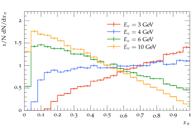
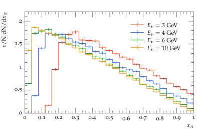
Figure 2: Momentum fraction of the outgoing pion for $\tau^{-}\rightarrow\pi^{-}\nu_{\tau}$ decays of various incoming neutrino energies. Results are shown for the full polarization calculation on the left and the left-handed polarization approximation ($P_{L}^{T}=1,P_{T}^{T}=0$) on the right.

We next consider the decays of the tau into the two pion and three pion states, which are dominated by the decay chain $\tau^{-}\to\nu_{\tau}\rho^{-}(\rho^{-}\to\pi^{-}\pi^{0})$ and $\tau^{-}\to\nu_{\tau}a_{1}^{-}(a_{1}^{-}\to\pi^{-}\pi^{-}\pi^{+}$ or $a_{1}^{-}\to\pi^{-}\pi^{0}\pi^{0})$ respectively.

For the case of the $\rho$ channel, we analyze the momentum fraction of the hadronic system ($x_{\rho}=p_{\rho}/p_{\tau}$) as well as the momentum fraction of the $\pi^{-}$ with respect to the $\rho$ ($z_{\pi}=p_{\pi^{-}}/p_{\rho}$). The results are shown in Fig. 3 and Fig. 4 respectively. Again, the full calculation is on the left of each plot and the assumption of a purely left-handed tau is on the right. We can see that there is a significant impact from including the correct polarization in the calculation. In the case of the $\rho$ momentum fraction, we see that our results approach the transverse curve for the $\rho$ from Fig. 1 as $E_{\nu}$ increases. This is expected since we are summing over the polarizations of the $\rho$, which are dominated by the transverse polarization.

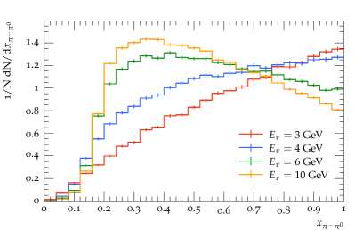
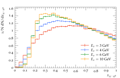
Figure 3: Momentum fraction of the $\pi^{-}\pi^{0}$ system for $\tau^{-}\rightarrow\pi^{-}\pi^{0}\nu_{\tau}$ decays of various incoming neutrino energies. Results are shown for the full polarization calculation on the left and the left-handed polarization approximation ($P_{L}^{T}=1,P_{T}^{T}=0$) on the right.

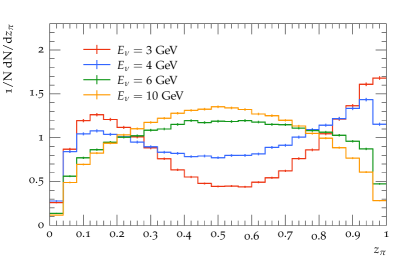
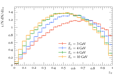
Figure 4: Ratio of the $\pi^{-}$ momentum to the $\rho^{-}$ momentum for $\tau^{-}\rightarrow\pi^{-}\pi^{0}\nu_{\tau}$ decays of various incoming neutrino energies, where $z_{\pi}$ denotes this ratio. Results are shown for the full polarization calculation on the left and the left-handed polarization approximation ($P_{L}^{T}=1,P_{T}^{T}=0$) on the right.

As mentioned in Sec. II.1, summing over the polarizations of the $a_{1}$ removes any sensitivity to the polarization of the $\tau$. Therefore, the $a_{1}$ momentum as a fraction of the $\tau$ momentum ($x_{a_{1}}=p_{a_{1}}/p_{\tau}$) should not show any difference between the full calculation and the left-handed only calculation. This is supported by Figs. 5 and 6, with the left and right panel being statistically consistent with each other. Figure 5 shows the decay to the $\pi^{+}\pi^{-}\pi^{-}$ final state and Fig. 6 shows the decay to the $\pi^{-}\pi^{0}\pi^{0}$ final state. Furthermore, the curves approach the result of the collinear limit as $E_{\nu}$ increases, as seen by comparing to the transverse $a_{1}$ curve of Fig. 1.

Finally, we consider the leptonic decay channel. Here we will focus on the decays to electrons due to the possible experimental relevance at DUNE for $\nu_{\tau}$ detection, but note that up to corrections from the muon mass and the difference in the branching ratios the predictions would be identical. The comparison for various neutrino energies is given in Fig. 7. Again, we can see a difference between the full calculation in the left panel and the purely left-handed calculation in the right panel. The latter result approaches the expected prediction for large $E_{\nu}$ as shown in Fig. 1.

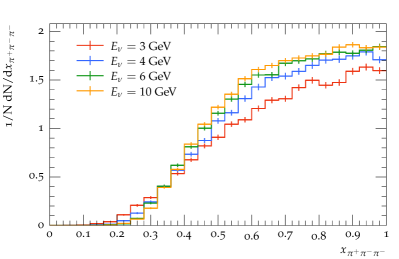
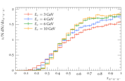
Figure 5: Momentum fraction of the $\pi^{+}\pi^{-}\pi^{-}$ system for $\tau^{-}\rightarrow\pi^{+}\pi^{-}\pi^{-}\nu_{\tau}$ decays of various incoming neutrino energies. Results are shown for the full polarization calculation on the left and the left-handed polarization approximation ($P_{L}^{T}=1,P_{T}^{T}=0$) on the right.

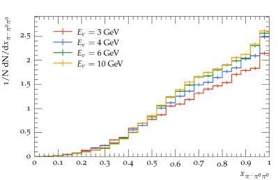
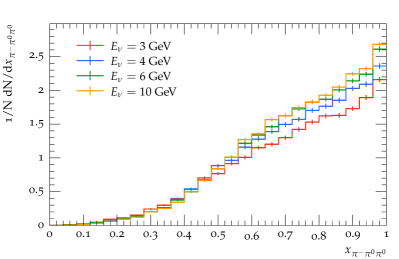
Figure 6: Momentum fraction of the $\pi^{-}\pi^{0}\pi^{0}$ system for $\tau^{-}\rightarrow\pi^{-}\pi^{0}\pi^{0}\nu_{\tau}$ decays of various incoming neutrino energies. Results are shown for the full polarization calculation on the left and the left-handed polarization approximation ($P_{L}^{T}=1,P_{T}^{T}=0$) on the right.

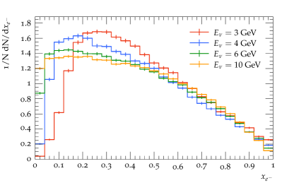
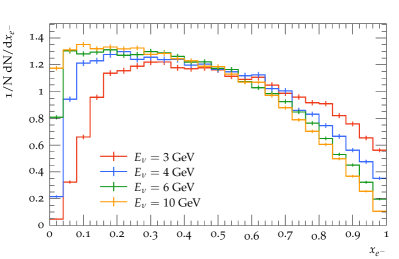
Figure 7: Momentum fraction of the outgoing electron for $\tau^{-}\rightarrow e^{-}\nu_{\tau}\bar{\nu}_{e}$ decays of various incoming neutrino energies. Results are shown for the full polarization calculation on the left and the left-handed polarization approximation ($P_{L}^{T}=1,P_{T}^{T}=0$) on the right.

IV.2 Realistic beams

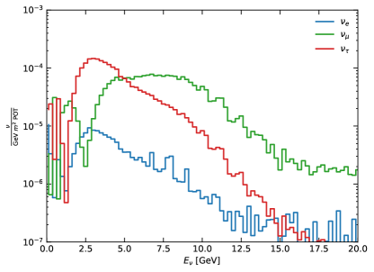
Figure 8: Neutrino flux in the far detector of DUNE. The flux is generated from running in $\tau$-optimized mode. The unoscillated fluxes are obtained from Ref. Fields .

To investigate the impact of spin-correlations in a more realistic setting, we consider the $\tau$-optimized flux mode for the DUNE experiment Fields . The oscillated far detector flux is shown in Fig. 8. The oscillation parameters are fixed to the values from the global fit de Salas et al. (2021):

$$\delta m_{21}^{2} =7.50\times 10^{-5}\ \textrm{eV}^{2},\quad\delta m_{31}^{2}=2.55\times 10^{-3}\textrm{eV}^{2},$$

$$s_{12}^{2} =0.318,\ s_{23}^{2}=0.574,\ s_{13}^{2}=0.0220,\ \delta_{CP}=1.08\pi\,.$$

The results are given using the flux averaged cross-section, defined as

$$\langle\sigma\rangle=\frac{\int{\rm d}E_{\nu}\Phi(E_{\nu})\sigma(E_{\nu})}{\int{\rm d}E_{\nu}\Phi(E_{\nu})}\,,$$ (22)

where $\Phi(E_{\nu})$ is the neutrino flux and $\sigma(E_{\nu})$ is the neutrino energy dependent cross- section.

While all possible decay channels are implemented, we consider here only those most affected by correctly handling polarization. Furthermore, only decay channels with sufficiently large branching ratios such that the differences are experimentally relevant are shown.

We first consider the single pion decay channel, since it is a clean channel to reconstruct at DUNE. The results of the calculation are shown in the left panel of Fig. 9. Here we see that in the full calculation, the outgoing pion tends to be more energetic than in the fully left-handed case.

The case of leptonic decays is shown in the right panel of Fig. 9, and is calculated in the massless limit for both the electron and the muon. In this case, the two decays are identical. The effect of including the full polarization information makes the outgoing lepton softer compared to the fully left-handed calculation. While the chance of detecting the muon channel is extremely difficult, there is a chance to detect the electron channel due to the low $\nu_{e}$ flux at the far detector as seen in Fig. 8.

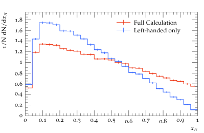
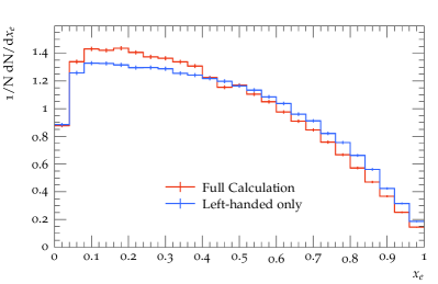
Figure 9: Momentum fraction distribution for the decay of the $\tau$ into a single pion is shown on the left and momentum fraction distribution for the decay into an electron is shown on the right. The full polarization handling is shown in red with the approximation that the $\tau$ is purely left-handed in blue. The predictions are folded over the DUNE far-detector flux running in the $\tau$-optimized mode given in Fig. 8.

Another interesting decay channel to consider is the two pion final state, which has the largest branching fraction of all decay channels. For this decay channel, we consider the momentum of the sum of the two pions as a fraction of the $\tau$ momentum ($x_{\pi\pi}$) and the momentum of the negatively charged pion as a fraction of the momentum sum ($z_{\pi}$). Figure 10 shows the difference between the full calculation in red and the fully left-handed approximation in blue. In the case of the $x_{\pi\pi}$ distribution, the total momentum is harder in the full calculation compared to the left-handed assumption. Additionally, there is a significant difference in $z_{\pi}$ between the full calculation and the left-handed only. The full calculation is relatively flat over the full range, while the left-handed only calculation is peaked around 0.6. This shift is significant, and will be important for any detailed study on using the two pion channel to detect tau neutrino events.

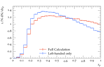
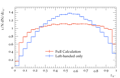
Figure 10: Momentum fraction distribution for the decay of the $\tau$ into a pair of pions is shown on the left. The momentum of the negatively charged pion as a fraction of the sum of the pion momenta is given on the right. The full polarization handling is shown in red with the approximation that the $\tau$ is purely left-handed in blue. The predictions are folded over the DUNE far-detector flux running in the $\tau$-optimized mode given in Fig. 8.

The last decay channel considered in this work is the decay to three pions. In this case, the decay is dominated by the $a_{1}$ meson as discussed in Sec. II.1, and since we are not separating out the $a_{1}$ polarization should not be sensitive to the polarization of the $\tau$. This can be seen in Fig. 11, where the decay $a_{1}\to\pi^{0}\pi^{0}\pi^{-}$ can be seen on the left and the decay $a_{1}\to\pi^{+}\pi^{-}\pi^{-}$ can be seen on the right. The full calculation and the left-handed only calculation are statistically consistent with each other, as expected.

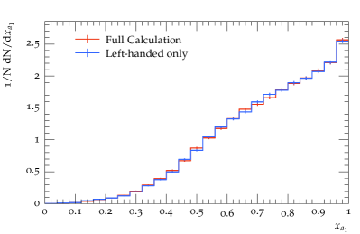
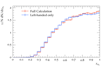
Figure 11: The full calculation (red) and the purely left-handed calculation (blue) are given for the momentum fraction of the three pions as a fraction of the total $\tau$ momentum for the decay of the $a_{1}$, with the $\pi^{0}\pi^{0}\pi^{-}$ channel on the left and the $\pi^{+}\pi^{-}\pi^{-}$ channel on the right. The predictions are folded over the DUNE far-detector flux running in the $\tau$-optimized mode given in Fig. 8.

Finally, we perform the analysis proposed in Ref. Machado et al. (2020). The comparison between the full calculation and the left-handed polarization assumption is shown in Fig. 12 for the energy of the leading pion. There is a shift in the energy distribution of the pion when correctly handling the tau polarization, making the pion slightly harder. The study on the impact of this in the separation from the neutral current background is left to a future work. Since the final state interactions are turned off in this analysis, the other distributions given in Ref. Machado et al. (2020) would not be accurate. Therefore, they are not included here but will be included in a detailed study on separating the $\tau$ decays from the background.

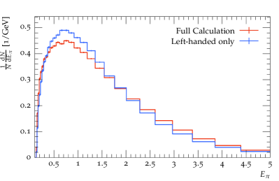
Figure 12: Energy of the leading pion in $\nu_{\tau}A\to\tau X$ events, in which all possible decays of the $\tau$ are included. These results do not include the production of pions from the intranuclear cascade.

V Conclusions

Due to the limited number of identifiable tau neutrino events, the tau neutrino is typically considered the least understood fundamental particle in the Standard Model. Current and next-generation experiments will collect a large number of tau neutrino events, opening the door to detailed study of this particle.

One of the most important experiments for studying the tau neutrino will be the DUNE experiment. It will be the only experiment using accelerator neutrinos for measuring properties of the tau neutrino. At DUNE energies, the quasielastic scattering component is the dominant contribution. In this energy region, there is an irreducible background from neutral current resonance interactions. Therefore, it is vital to understand the most optimal way to separate the signal from the background. Traditionally, in neutrino event generators the outgoing $\tau$ is assumed to be fully left-hand polarized. This assumption is poor for DUNE energies.

In this work, we demonstrate the appropriate way of calculating the polarization of the tau and propagating this information through the full decay chain within an event generator framework. The simulations were performed with a publicly available version of Achilles interfaced with Sherpa. For validation, we showed that the distributions for single pion are consistent with Ref. Hernández et al. (2022) for monochromatic beams. We additionally showed strong shifts in the momentum distributions for the two pion decay channel and found insignificant shifts (as expected) in the three pion decay channels from the fully left-handed assumption. We also considered the decay in the leptonic channel, and found a slight shift when correctly handling the polarization.

While the study with monochromatic beams allows for validation of the calculation, all current and future experiments have a broad spread in the neutrino energies. We therefore investigated the changes in the same distributions integrated over the $\tau$-optimized running mode for DUNE. Again we find significant changes from the traditional fully left-handed assumption in the lepton, single pion, and two pion channel. As expected, there were no significant modifications in the three pion channel.

Finally, while the distributions shown here demonstrate the importance of properly handling the polarization of the tau, they are not necessarily the optimal variables for separating the tau from the neutral current background. The investigation of how to optimally separate the charge current tau neutrino interactions from the SM background is left to a future work.

VI Acknowledgments

We thank Joanna Sobczyk and collaborators for insightful discussions. We thank Noemi Rocco, William Jay, and André de Gouvêa for many useful discussions and for their comments on the manuscript. We thank Pedro Machado for helping with the realistic tau neutrino beams, for many fruitful discussions, and for his comments on the manuscript. This manuscript has been authored by Fermi Research Alliance, LLC under Contract No. DE-AC02-07CH11359 with the U.S. Department of Energy, Office of Science, Office of High Energy Physics.

References

- Kodama et al. (2001) K. Kodama et al. (DONUT), Phys. Lett. B 504, 218 (2001), arXiv:hep-ex/0012035 .
- Kodama et al. (2008) K. Kodama et al. (DONuT), Phys. Rev. D 78, 052002 (2008), arXiv:0711.0728 [hep-ex] .
- Agafonova et al. (2018) N. Agafonova et al. (OPERA), Phys. Rev. Lett. 120, 211801 (2018), [Erratum: Phys.Rev.Lett. 121, 139901 (2018)], arXiv:1804.04912 [hep-ex] .
- Li et al. (2018) Z. Li et al. (Super-Kamiokande), Phys. Rev. D 98, 052006 (2018), arXiv:1711.09436 [hep-ex] .
- Aartsen et al. (2019) M. G. Aartsen et al. (IceCube), Phys. Rev. D 99, 032007 (2019), arXiv:1901.05366 [hep-ex] .
- Abbasi et al. (2022) R. Abbasi et al. (IceCube), Eur. Phys. J. C 82, 1031 (2022), arXiv:2011.03561 [hep-ex] .
- De Gouvêa et al. (2019) A. De Gouvêa, K. J. Kelly, G. V. Stenico, and P. Pasquini, Phys. Rev. D 100, 016004 (2019), arXiv:1904.07265 [hep-ph] .
- Abi et al. (2020) B. Abi et al. (DUNE), (2020), arXiv:2002.03005 [hep-ex] .
- Ishihara (2021) A. Ishihara (IceCube), PoS ICRC2019, 1031 (2021), arXiv:1908.09441 [astro-ph.HE] .
- Feng et al. (2023) J. L. Feng et al., J. Phys. G 50, 030501 (2023), arXiv:2203.05090 [hep-ex] .
- Esteban et al. (2021) I. Esteban, S. Pandey, V. Brdar, and J. F. Beacom, Phys. Rev. D 104, 123014 (2021), arXiv:2107.13568 [hep-ph] .
- Argüelles et al. (2020) C. A. Argüelles, M. Bustamante, A. Kheirandish, S. Palomares-Ruiz, J. Salvado, and A. C. Vincent, PoS ICRC2019, 849 (2020), arXiv:1907.08690 [astro-ph.HE] .
- Mammen Abraham et al. (2022) R. Mammen Abraham et al., J. Phys. G 49, 110501 (2022), arXiv:2203.05591 [hep-ph] .
- Sobczyk et al. (2019) J. E. Sobczyk, N. Rocco, and J. Nieves, Phys. Rev. C 100, 035501 (2019), arXiv:1906.05656 [nucl-th] .
- Hernández et al. (2022) E. Hernández, J. Nieves, F. Sánchez, and J. E. Sobczyk, Phys. Lett. B 829, 137046 (2022), arXiv:2202.07539 [hep-ph] .
- Machado et al. (2020) P. Machado, H. Schulz, and J. Turner, Phys. Rev. D 102, 053010 (2020), arXiv:2007.00015 [hep-ph] .
- Andreopoulos et al. (2010) C. Andreopoulos et al., Nucl. Instrum. Meth. A 614, 87 (2010), arXiv:0905.2517 [hep-ph] .
- Golan et al. (2012) T. Golan, J. T. Sobczyk, and J. Zmuda, Nucl. Phys. B Proc. Suppl. 229-232, 499 (2012).
- Hayato and Pickering (2021) Y. Hayato and L. Pickering, Eur. Phys. J. ST 230, 4469 (2021), arXiv:2106.15809 [hep-ph] .
- Leitner et al. (2006) T. Leitner, L. Alvarez-Ruso, and U. Mosel, Phys. Rev. C 73, 065502 (2006), arXiv:nucl-th/0601103 .
- Chrzaszcz et al. (2018) M. Chrzaszcz, T. Przedzinski, Z. Was, and J. Zaremba, Comput. Phys. Commun. 232, 220 (2018), arXiv:1609.04617 [hep-ph] .
- Isaacson et al. (2023) J. Isaacson, W. I. Jay, A. Lovato, P. A. N. Machado, and N. Rocco, Phys. Rev. D 107, 033007 (2023), arXiv:2205.06378 [hep-ph] .
- Gleisberg et al. (2004) T. Gleisberg, S. Höche, F. Krauss, A. Schälicke, S. Schumann, and J. Winter, JHEP 02, 056 (2004), hep-ph/0311263 .
- Gleisberg et al. (2009) T. Gleisberg, S. Höche, F. Krauss, M. Schönherr, S. Schumann, F. Siegert, and J. Winter, JHEP 02, 007 (2009), arXiv:0811.4622 [hep-ph] .
- Bothmann et al. (2019) E. Bothmann et al. (Sherpa), SciPost Phys. 7, 034 (2019), arXiv:1905.09127 [hep-ph] .
- Isaacson et al. (2022) J. Isaacson, S. Höche, D. Lopez Gutierrez, and N. Rocco, Phys. Rev. D 105, 096006 (2022), arXiv:2110.15319 [hep-ph] .
- Christensen and Duhr (2009) N. D. Christensen and C. Duhr, Comput. Phys. Commun. 180, 1614 (2009), arXiv:0806.4194 [hep-ph] .
- Alloul et al. (2014) A. Alloul, N. D. Christensen, C. Degrande, C. Duhr, and B. Fuks, Comput.Phys.Commun. 185, 2250 (2014), arXiv:1310.1921 [hep-ph] .
- Bullock et al. (1993) B. K. Bullock, K. Hagiwara, and A. D. Martin, Nucl. Phys. B 395, 499 (1993).
- Martin and Spearman (1970) A. D. Martin and T. D. Spearman, Elementary Particle Theory (North-Holland Publishing Co., Amsterdam, 1970).
- Valverde et al. (2006) M. Valverde, J. E. Amaro, J. Nieves, and C. Maieron, Phys. Lett. B 642, 218 (2006), arXiv:nucl-th/0606042 .
- (32) T. Laubrich, Diploma Thesis.
- (33) F. Siegert, Diploma thesis.
- Workman et al. (2022) R. L. Workman et al. (Particle Data Group), PTEP 2022, 083C01 (2022).
- Kühn, Johann H. and Santamaría, A. (1990) Kühn, Johann H. and Santamaría, A., Z. Phys. C48, 445 (1990).
- Ecker et al. (1989) G. Ecker, J. Gasser, A. Pich, and E. de Rafael, Nucl. Phys. B321, 311 (1989).
- Richardson (2001) P. Richardson, JHEP 11, 029 (2001), arXiv:hep-ph/0110108 .
- Gleisberg and Höche (2008) T. Gleisberg and S. Höche, JHEP 12, 039 (2008), arXiv:0808.3674 [hep-ph] .
- Höche et al. (2015) S. Höche, S. Kuttimalai, S. Schumann, and F. Siegert, Eur. Phys. J. C75, 135 (2015), arXiv:1412.6478 [hep-ph] .
- Degrande et al. (2012) C. Degrande, C. Duhr, B. Fuks, D. Grellscheid, O. Mattelaer, and T. Reiter, Comput.Phys.Commun. 183, 1201 (2012), arXiv:1108.2040 [hep-ph] .
- Benhar et al. (1994) O. Benhar, A. Fabrocini, S. Fantoni, and I. Sick, Nucl. Phys. A 579, 493 (1994).
- Kelly (2004) J. J. Kelly, Phys. Rev. C 70, 068202 (2004).
- (43) L. Fields, “DUNE Fluxes,” .
- de Salas et al. (2021) P. F. de Salas, D. V. Forero, S. Gariazzo, P. Martínez-Miravé, O. Mena, C. A. Ternes, M. Tórtola, and J. W. F. Valle, JHEP 02, 071 (2021), arXiv:2006.11237 [hep-ph] .