The Random Hivemind: An Ensemble Deep Learner.
A Case Study of Application to Solar Energetic Particle Prediction Problem.

Abstract

Deep learning has become a popular trend in recent years in the machine learning community and has even occasionally become synonymous with machine learning itself thanks to its efficiency, malleability, and ability to operate free of human intervention. However, a series of hyperparameters passed to a conventional neural network (CoNN) may be rather arbitrary, especially if there is no surefire way to decide how to program hyperparameters for a given dataset. The random hivemind (RH) alleviates this concern by having multiple neural network estimators make decisions based on random permutations of features. The learning rate and the number of epochs may be boosted or attenuated depending on how all features of a given estimator determine the class that the numerical feature data belong to, but all other hyperparameters remain the same across estimators. This allows one to quickly see whether consistent decisions on a given dataset can be made by multiple neural networks with the same hyperparameters, with random subsets of data chosen to force variation in how data are predicted by each, placing the quality of the data and hyperparameters into focus. The effectiveness of RH is demonstrated through experimentation in the predictions of dangerous solar energetic particle events (SEPs) by comparing it to that of using both CoNN and the traditional approach used by ensemble deep learning in this application. Our results demonstrate that RH outperforms the CoNN and a committee-based approach, and demonstrates promising results with respect to the “all-clear” prediction of SEPs.

1 Introduction

The Prediction of Solar Energetic Particle events (SEPs) and the understanding of their precursors represent major challenges in heliophysics and space weather from both the operational and the research perspectives. Increased fluxes of SEPs are of interest to various users, from governmental and private space weather agencies to airlines and power grid operators. Routine daily forecasting and a shorter-term warning and alerts system for the major subclass of SEPs, the Solar Proton Events (SPEs), was implemented, for example, by Space Weather Prediction Center at National Oceanic and Atmospheric Administration (SWPC NOAA, Balch, 1999, 2008). The performance of this operational forecasting system was recently analyzed by Bain et al. (2021) and, although it had improved from the solar cycle 23 to the solar cycle 24 in general, yet far from capturing every single SEP event ahead of time.

The statistical relations between the flare soft X-ray properties (such as the peak ratios of the 1-8$\AA$ and 0.5-4$\AA$ fluxes, which is similar to the temperature computed in a single-temperature approximation, Ryan et al., 2012; Sadykov et al., 2019) and the consequent CMEs and SEPs have been known for a long time. In particular, it found that the lower the considered soft X-ray class of the flare is, more is the difference in the peak temperature between the SEP-associated and SEP-quiet flares, with lower temperatures corresponding to SEP-associated flares (Garcia, 1994). These relations were quantified and utilized for forecasting SEP on larger statistics of the events (Garcia, 2004). The results were also reproduced later (Kahler & Ling, 2018), where the authors attempted to predict the SEP-associated flares using the k-nearest neighbors machine learning algorithm and neural networks separately for the Western and Eastern hemispheres. In addition, the durations and temperatures of the flares were found to be related statistically to the properties of the CMEs (Ling & Kahler, 2020; Kahler & Ling, 2022) which can, subsequently, be used to constrain SEP parameters Kahler & Vourlidas (2013) or serve as a basis for establishing empirical models for SEP forecasting (Richardson et al., 2018).

The extension of these works is the employment of machine learning (ML), and deep learning techniques in particular, for forecasting SEPs based on the properties of the preceding (parental, host) solar flares. For example, Aminalragia-Giamini et al. (2021) employed neural networks trained on the time series of the GOES soft X-ray fluxes during the solar flares directly. The authors found that the model is able to predict the large majority of SEP-associated flares (higher than 85%) during the considered time period of 1988-2013 while maintaining a low false-positive rate. The Empirical model for Solar Proton Event Real Time Alert (ESPERTA, Laurenza et al., 2009, 2018) forecasting tool provides short-term predictions of $>$ 10 MeV and $>$ 100 MeV SPEs. Although not based on machine learning directly, the method relies on the properties of the host flare and follows a well-defined decision tree for forecasting SEPs. Boubrahimi et al. (2017) decision tree ML model to also analyze GOES soft X-ray and proton flux time series for prediction of $>$100 MeV SPEs. Lavasa et al. (2021) analyzed a variety of ML algorithms (such as random forest, neural networks, extremely randomized trees, and extreme gradient boosting) and concluded that, among the soft X-ray parameters, the fluence is the most important for the prediction of SEPs.

One of the challenges related to the prediction of SEP events is that these events are rare and will represent minority-class events for the classification problem. For example, the number of days with the enhanced flux of $\geq{}10\,MeV$ protons (determined as being $\geq{}10\,pfu$ to the number of days with no enhanced flux is $\sim{}1/23$ for the solar cycles 22-24 (Ali et al., 2023) and is even more extreme $\sim{}1/34$ it the solar cycle 24 only is considered (Sadykov et al., 2021). It was concluded for the aforementioned ESPERTA model (Stumpo et al., 2021) that the performance of the algorithm (specifically, the False Alarm Rate, FAR) depends on the class-imbalance ratio in the train data set. Various techniques can be implemented to deal with the class-imbalanced data, such as oversampling, undersampling, and misclassification weights (Ahmadzadeh et al., 2021) or generation of the synthetic data (Chen et al., 2021). On the other hand, in addition to the traditional data-centric approaches to dealing with class imbalance, the ensemble classifiers can be employed in such problems (Galar et al., 2012). With respect to the problem of the prediction of SEPs, promising results were previously obtained for neural network-based “committee” ensembles (Aminalragia-Giamini et al., 2021) and random forest ensemble algorithm (Lavasa et al., 2021).

In our previous work, we have presented the application of the random forest ML algorithm for the prediction of SEPs and tested various class-imbalance treatment techniques (O’Keefe et al., 2022). In this work, we expand our investigation to new types of ML algorithms, including Conventional Neural Networks (CoNN), an ensemble of CoNNs following a voting approach (“Committee”, Aminalragia-Giamini et al., 2021), and introduce a weighted consensus that we call a Random Hivemind (RH). Both ensemble approaches considered are so-called “bagging” ensemble classifiers, when individual ensemble members do not depend on each other and deterministically contribute to the classification decision. Investigation of the relative performance of the algorithms on the given data set of flares associated with SEPs is the primary focus of this paper. The paper is structured as follows. Section 2 describes the data preparation employed in this paper, namely the processing of the soft X-ray data, an association of flares and SEPs, and the preparation of data sets ready for ML. Section 3 describes the ML algorithms tested in this work. The results and discussion are presented in Section 4 and followed by the conclusion in Section 5.

2 Data Preparation

The soft X-ray emission in 0.5-4 $\AA$ and 1-8 $\AA$ wavelength channels can be represented under a single-temperature plasma approximation by two parameters, namely the plasma temperature (T) and its emission measure (EM). We are utilizing the T and EM values estimated using the Temperature and Emission measure Based Background Subtraction algorithm (TEBBS, Ryan et al., 2012; Sadykov et al., 2017) and collected in the Interactive Multi-Instrument Database of Solar Flares (IMIDSF, Sadykov et al., 2017, https://data.nas.nasa.gov/helio/portals/solarflares/) for 2002-2017 time period. In addition to peak values of the temperature and emission measure, $T_{max}$ and $EM_{max}$, we are utilizing the background-subtracted flare classes ($SXR_{max}$), flare durations, and time differences between the $T_{max}$, $EM_{max}$, and $SXR_{max}$ times to the flare start and end times, which sums up to the 10 parameters for every flare. After the exclusion of the flares with $T_{max}=100$ MK and the negative time differences between the flare end times and $T_{max}$, $EM_{max}$, and $SXR_{max}$ times (which appear because of the TEBBS algorithm implementation issues) our data set contained 24574 flares. This includes 3 A-class, 10536 B-class, 12600 C-class, 1312 M-class, and 109 X-class flares according to GOES classification after TEBBS background subtraction.

To associate the flares with the SEP records, we are utilizing the list of the Solar Proton Events Affecting the Earth Environment provided by the Space Environment Services Center of the National Oceanic and Atmospheric Administration (NOAA). The SEPs in this data set represent the events when the flux of $>$10 MeV particles measured by the Geostationary Operational Environmental Satellite (GOES) is larger than 10 pfu in its peak. If the flare event caused the SEP event sometime in the future according to this list, the corresponding flare event is marked as a positive instance; otherwise, it is marked as a negative instance. Such association results in a total of 74 flares associated with SEPs, and 24,500 negative flare instances, providing an extreme class-imbalance ratio of  1/331. The distribution of some of the parameters of these flares is presented in Figure 1. In terms of the $SXR_{max}$ parameter, 11 of the SEPs corresponded to the C-class flares, 41 — to M-class, and 22 — to X-class (after the TEBBS background subtraction). The list of the studied flares is publicly available at the Solar Energetic Particle Prediction Portal (SEP³) webpage.

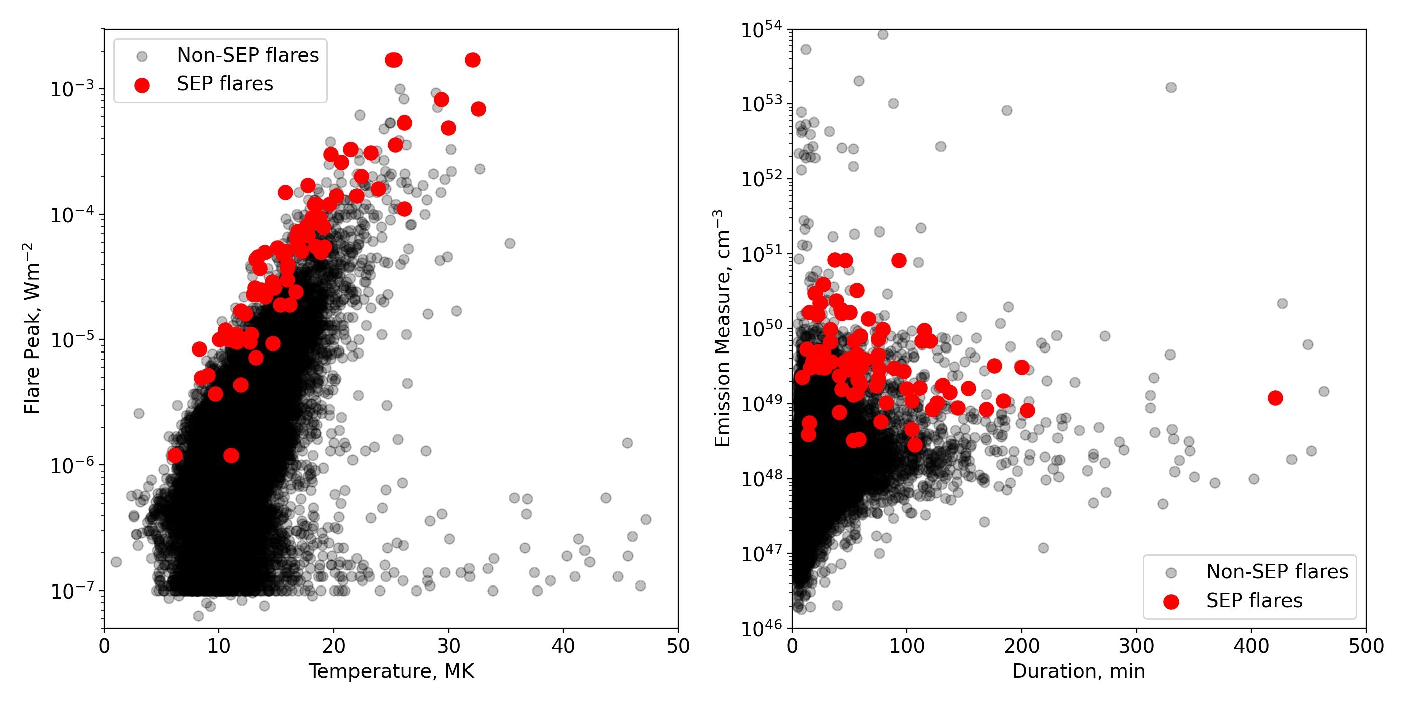
Figure 1: Distribution of the flare peak emissions at 1-8 $\AA$ and flare peak temperatures (left), and flare durations and peak emission measures (right). Solar flares that did not result in the following SEP event are marked in black, and that resulted are marked in red.

One can see in Figure 1 that the flares that resulted in SEPs are not distributed randomly even among the flares of the same SXR peak fluxes. Specifically, the left panel in Figure 1 indicates that SEP-associated flares are colder on average among the flares of the same SXR peak flux (or flare class). The same dependence was observed by Garcia (1994, 2004). After the data set is constructed, we subdivide the data set into training and testing subsets, the latter being 0.3 the size of the original dataset. The train-test separation was repeated 10 times for every machine learning experiment presented in this paper.

3 Machine Learning Methodology

Three neural network-based approaches are considered in this paper for the problem of prediction of SEP events. The first is the conventional neural network (hereafter CoNN) which represents the fully-connected neural network architecture. For ensemble deep learners, two more neural network-based approaches are constructed. The first ensemble approach is the traditional “Committee” scheme that involves using a series of multiple neural network estimators with the same input features and input layer shapes. The second ensemble approach is a Random Hivemind (RH) which is built using random permutations of features from the training data as input features. For the series of tests presented in this paper, the square root of the total number of features, rounded up, is chosen as the number of input features for each neural network within an RH and the layout between estimators remains unchanged within each “Committee”. Correspondingly, one has 10 features entering the CoNN or each committee member, and 4 features selected using the procedure described below entering the RH classifier. Each ensemble setup has 10 neural network estimators. The architectures of the utilized ML methods are schematically illustrated in Figure 2.

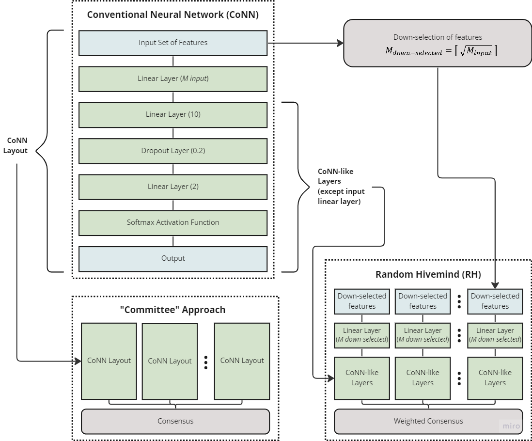
Figure 2: The schematic representation of the layouts of the Conventional Neural Network (CoNN), “Committee” Network, and Random Hivemind Network (RH). The numbers in parentheses for the linear layers indicate the number of neurons in the layer, and the number in parentheses for the dropout layer indicates the probability of each connection/weight being dropped from the training procedure.

The random permutations of features are chosen by first computing the $\chi$-squared statistics between the features and the SEP class to assign scores to each feature based on how significant each is in determining whether or not a given flare caused a SEP. The scores from applying the $\chi$-squared test to the features are normalized so that the sum of these new scores (“feature weights”) equals one. The feature weights are then used as the probabilities that given features with their respective weights will be chosen to be used in an RH estimator.

Each neural network, including CoNN, Committee estimators, and RH estimators, has an input layer equal to the number of features being tested by the said estimator, a dense layer with an input and output shape of 10, a dropout layer with a probability of 0.2, and an output layer with an output shape equal to the number of predicted features. The numbers of epochs and learning rates for all neural CoNN and committee setups are kept at their default values of $n_{epochs}=10$ and $\alpha{}=0.01$ respectively, whereas RH boosts its epoch counts and learning rates using these formulae:

$$n_{epochs}=10\times{}(2-x)$$ (1)

$$\alpha=0.01\times{}(\eta+xe^{x-1})$$ (2)

Here $x$ is the total sum of feature weights for a given estimator, $n_{epochs}$ is the number of epochs during the training process, $\alpha$ is the learning rate, and $e$ is the base of the natural logarithm. The parameter $\eta{}=ex\Sigma{}x/n_{features}$, where $n_{features}$ is the number of features selected for the given estimator, and $\Sigma{}x$ is the total weight of features in all estimators within the ensemble. Outcomes are predicted by putting prediction data through each of the estimators constructed during the training phase and seeing what each estimator chooses as a predicted result. Each committee considers all results by all estimators as equal, using a simple plurality vote to determine which class a given datum belongs to. Each RH considers each estimator’s value in a classification vote as equal to the sum of the feature weights said estimator’s input features have.

Let us consider an example of feature weights in more detail. If a given flare’s SXR peak flux had a feature weight of $0.25$, its emission measure peak value had one of $0.1$, its temperature peak value had one of $0.05$, and its duration had one of $0.01$, the peak SXR flux would have a probability of $0.25$ of being chosen to be in an RH estimator, the emission measure peak flux would have one of $0.1$, etc. A CoNN and a “committee”, however, would consider all available features equally to be chosen as input features. During training, an RH estimator that uses all four of these parameters would go through 15 epochs with a learning rate of approximately $\alpha=0.0115$. A CoNN and a “committee” estimator in this example, however, would each only go through 10 epochs with a learning rate of $\alpha=0.01$, since they do not have the ability to be able to automatically calculate these parameters based on feature selection. When deciding, each RH estimator would use the sums of its feature weights as values, so an estimator with these four parameters would have a value of 0.5 when voting. Each “committee” estimator would have a value of 1, since, again, no mechanism exists to determine how to calculate these figures based on feature selection.

For all neural networks, including CoNN, “committee” estimators, and RH estimators, the Adam optimizer is used, and overfit prevention measures including dropout layers with probabilities of 0.2 and data shuffling are used. Only flares between soft X-ray classes C4.0 and M3.3 are chosen for training since they are the more ambiguous cases that all learners need to focus on the most (O’Keefe et al., 2022). This is determined by finding the ”liar’s poker threshold” mentioned in the paper, which represents the peak X-ray flux value above which the proportion of the total number of SPE-active flares exceeds that of the SPE-quiet flares in relation to the numbers of flares in each class, and then finding the corresponding thresholds above and below the prior threshold. Flares of any class are available for use as testing data.

To classify prediction data, an RH classifier chooses the result that the highest number of estimators reach. In this case, flares are classified into SPE-active and SPE-quiet. All neural networks involved have balanced class weights in their cross-entropy loss functions when used as classifiers. Metrics used to compare classification methods include accuracy, balanced accuracy, true skill score (TSS), and Heidke skill score 2 (HSS). For a definition of these metrics see, for example, (Bobra & Couvidat, 2015). We also utilize the area under the Received Operating Characteristic curve (ROC_AUC), precision, and recall. In addition, we demonstrate the individual elements of the confusion matrix (true positive predictions, $TP$, true negative predictions, $TN$, false positive predictions, $FP$, and false negative predictions, $FN$) for each approach averaged over the 10 random train-test splits.

4 Results and Discussion

The results of the classification algorithms employed in this study in terms of confusion matrix elements and various prediction scores are presented in Table 1 (summary results for all classifiers as the average scores and standard deviations), Table 2 (summary results for all classifiers as the median scores and median absolute deviations) and Tables 3, 4, and 5 (results for individual tests for each classifier).

Algorithm / Metrics	CoNN	Committee	RH
TN	5975.9$\pm$1025.2	6081.0$\pm$321.7	6249.2$\pm$381.9
FP	1371.8$\pm$1024.9	1266.7$\pm$323.5	1098.5$\pm$381.8
FN	4.9$\pm$7.9	1.7$\pm$2.5	0.9$\pm$1.5
TP	18.4$\pm$9.0	21.6$\pm$3.5	22.4$\pm$9.3
Precision	0.016$\pm$0.010	0.018$\pm$0.006	0.022$\pm$0.007
Recall	0.78$\pm$0.35	0.93$\pm$0.11	0.96$\pm$0.07
Accuracy	0.81$\pm$0.14	0.83$\pm$0.04	0.85$\pm$0.05
Balanced Accuracy	0.78$\pm$0.15	0.88$\pm$0.06	0.91$\pm$0.04
TSS	0.60$\pm$0.31	0.76$\pm$0.12	0.81$\pm$0.08
HSS	0.025$\pm$0.019	0.029$\pm$0.011	0.036$\pm$0.013
ROC_AUC	0.79$\pm$0.32	0.94$\pm$0.04	0.96$\pm$0.02

Table 1: Average values and standard deviations of the performances of the classifiers considered in this paper.

Algorithm / Metrics	CoNN	Committee	RH
TN	6220.0$\pm$488.5	6182.5$\pm$209.0	6405.0$\pm$134.0
FP	1128.5$\pm$447.0	1167.0$\pm$210.5	942.0$\pm$133.0
FN	0.0$\pm$0.0	0.5$\pm$0.5	0.5$\pm$0.5
TP	23.0$\pm$3.5	23.0$\pm$1.5	24.0$\pm$2.5
Precision	0.014$\pm$0.005	0.019$\pm$0.005	0.023$\pm$0.005
Recall	1.0$\pm$0.0	0.98$\pm$0.02	0.98$\pm$0.02
Accuracy	0.85$\pm$0.06	0.84$\pm$0.03	0.87$\pm$0.02
Balanced Accuracy	0.87$\pm$0.07	0.89$\pm$0.03	0.92$\pm$0.02
TSS	0.74$\pm$0.15	0.79$\pm$0.16	0.84$\pm$0.03
HSS	0.022$\pm$0.009	0.031$\pm$0.009	0.039$\pm$0.010
ROC_AUC	0.98$\pm$0.01	0.95$\pm$0.02	0.97$\pm$0.01

Table 2: Median values and median absolute deviations (computed as median values of the absolute deviations of the individual scores from the median) of the performances of the classifiers considered in this paper.

#	TN	FP	FN	TP	Precision	Recall	Accuracy	Balanced Accuracy	TSS	HSS	ROC_AUC
1	5866	1478	0	27	0.0179	1.0	0.7995	0.8994	0.7987	0.0283	0.985
2	3430	3919	0	22	0.0055	1.0	0.4683	0.7334	0.4667	0.0052	0.9915
3	6210	1137	0	24	0.0207	1.0	0.8457	0.9226	0.8452	0.0343	0.9825
4	5299	2046	0	26	0.0125	1.0	0.7224	0.8607	0.7214	0.0179	0.9798
5	6974	375	18	4	0.0106	0.1818	0.9467	0.5654	0.1308	0.0144	0.3023
6	5874	1470	1	26	0.0174	0.9630	0.8004	0.8814	0.7628	0.0271	0.9802
7	6230	1120	11	10	0.0088	0.4762	0.8466	0.6619	0.3238	0.0118	0.5077
8	6347	1008	0	16	0.0156	1.0	0.8632	0.9315	0.863	0.0266	0.9868
9	6763	584	0	24	0.0395	1.0	0.9208	0.9603	0.9205	0.0701	0.9891
10	6766	581	19	5	0.0085	0.2083	0.9186	0.5646	0.1293	0.0102	0.2028

Table 3: Performance metrics of the Conventional Neural Network (CoNN) classifier. The rows correspond to different experiments, the columns correspond to different forecast outcomes or metrics.

#	TN	FP	FN	TP	Precision	Recall	Accuracy	Balanced Accuracy	TSS	HSS	ROC_AUC
1	6407	937	4	23	0.0240	0.8519	0.8723	0.8621	0.7243	0.0398	0.9208
2	5563	1786	7	15	0.0083	0.6818	0.7567	0.7194	0.4388	0.0106	0.851
3	6323	1024	0	24	0.0229	1.0	0.8611	0.9303	0.8606	0.0387	0.988
4	6421	924	1	25	0.0263	0.9615	0.8745	0.9179	0.8357	0.0447	0.9518
5	5842	1507	1	21	0.0137	0.9545	0.7954	0.8747	0.7495	0.0213	0.9532
6	6272	1072	4	23	0.0210	0.8519	0.854	0.8529	0.7059	0.0341	0.8904
7	5599	1751	0	21	0.0119	1.0	0.7624	0.8809	0.7618	0.0179	0.9375
8	6093	1262	0	16	0.0125	1.0	0.8288	0.9142	0.8284	0.0205	0.97
9	5989	1358	0	24	0.0174	1.0	0.8158	0.9076	0.8152	0.0279	0.9777
10	6301	1046	0	24	0.0224	1.0	0.8581	0.9288	0.8576	0.0377	0.951

Table 4: Same as Table 3 but for the “Committee” classification approach.

#	TN	FP	FN	TP	Precision	Recall	Accuracy	Balanced Accuracy	TSS	HSS	ROC_AUC
1	5304	2040	0	27	0.0131	1.0	0.7232	0.8611	0.7222	0.0187	0.9578
2	6050	1299	1	21	0.0159	0.9545	0.8236	0.8889	0.7778	0.0256	0.9161
3	6248	1099	0	24	0.0214	1.0	0.8509	0.9252	0.8504	0.0357	0.9602
4	6477	868	1	25	0.0280	0.9615	0.8821	0.9217	0.8434	0.0479	0.984
5	6525	824	1	21	0.0249	0.9545	0.8881	0.9212	0.8424	0.0429	0.9517
6	6440	904	1	26	0.0280	0.9630	0.8772	0.9199	0.8399	0.0476	0.9754
7	6370	980	5	16	0.0161	0.7619	0.8664	0.8143	0.6286	0.026	0.9354
8	6030	1325	0	16	0.0119	1.0	0.8202	0.9099	0.8199	0.0194	0.9732
9	6553	794	0	24	0.0293	1.0	0.8923	0.946	0.8919	0.051	0.9868
10	6495	852	0	24	0.0274	1.0	0.8844	0.942	0.884	0.0473	0.9795

Table 5: Same as Table 3 but for the Random Hivemind (RH) classification approach.

There are several patterns in the forecasting scores evident from these tables. First, there is a striking difference between the scores and values of the confusion matrix elements obtained for the individual tests for the CoNN classifier. This is evident in Table 3 where the tests #5, #7, and #10 were accompanied by more than a half of SEP-active flares classified as non-SEP-active flares (correspondingly, following the condition $FN>TP$). Such behavior was rarely observed for the ensemble approaches (both the committee and RH) and resulted in noticeable differences between the mean and median scores for the CoNN classifier (for example, the mean values for the $TSS$ score for the CoNN classified was $TSS=0.60\pm{}0.31$ while the median value was $TSS=0.74\pm{}0.15$). Table 1 shows as well that the ensemble results typically have a much smaller standard deviation of the scores across the train-test pairs (which is especially evident for the confusion matrix elements and measures like $TN$, $FN$, Balanced accuracy, $TSS$, etc). Overall, such behavior indicates the robustness of the ensemble approaches with respect to the random train-test splits for the data set, while the training of the individual classifiers may fail. Therefore, the increase in the complexity of these ensemble algorithms is justified by their robust performance on the imbalanced data sets (Galar et al., 2012).

Tables 1 and 2 also indicate that the ensemble approaches are noticeably better than the CoNN classifiers with respect to the measures typically used in space weather forecasting, $HSS$ and $TSS$, both in terms of the mean and median values. The $TSS$ score had its median value of $TSS=0.74$ for CoNN classifier and increased to $TSS=0.79$ and $TSS=0.84$ for the committee and RH ensemble classifier. Although the $HSS$ scores were low, they still demonstrated an increase from $HSS=0.022$ to $HSS=0.031$ and $HSS=0.039$ when transitioning from the CoNN to ensembles. This demonstrates that the ensemble approaches are performing better, on average, with respect to the CoNN classifier, and are again more robust with respect to the random train-test separation of the data set, for the SEP forecasting purposes. The good performance of the ensemble classifiers was previously noticed in the works of Aminalragia-Giamini et al. (2021, for the committee approach) and Lavasa et al. (2021, for the random forest classifier). Interestingly, the case performances of the CoNN classifier, as row #9 in Table 3 demonstrates, may even outperform the individual ensemble classifier tests, which demonstrates the importance of evaluation of the methods on several train-test splits and demonstration of its robustness with respect to the random splitting.

Table 2 demonstrates that the RH classifier consistently outperforms the “committee” and CoNN approaches (except, probably, the number of $FN$ predictions whose median value was lower for CoNN, recall, and the area under the ROC curve). Also, the consistency of the results of individual tests of the RH classifier is better: the median absolute deviations are typically either smaller or comparable to the other two approaches. The key difference between the RH and the committee classifier is in the selection of features used for each individual ensemble member. While the committee members use all features available, RH members use the down-selected number of features (4 out of 10 in our case) and use the deterministic algorithm of the contribution of each committee member to the final result. We may assume that the down-selection of features for each member increases the forecasting scores because it helps to filter out the attention of the individual committee member to the noisy or irrelevant features. This confirms the importance of the feature selection process, which remains to be an active topic in the prediction of solar transient events (Bobra & Couvidat, 2015; Sadykov & Kosovichev, 2017; Yeolekar et al., 2021). Also, although the committee approach (Aminalragia-Giamini et al., 2021) helps to reduce the “reliance on chance” in terms of the convergence of the network parameters (weights and biases) to the local or global minima, it still contains similarly-structured CoNN networks as ensemble members. The RH introduces a more diverse population of ensemble members with the variable down-selected set of features as an input which can be more beneficial than having full-scale but nearly identical learners.

Here we notice another benefit of considering the RH approach for ML classification or regression tasks. While CoNNs are very flexible and malleable in how they train on new data, the parameters they are provided for aspects such as the size and shape of a given model, hyperparameters, and model selection, may need to be adjusted to be used on other data sets. This comes with the consequence of a requirement to continuously retrain models as data becomes more and more outdated or if new features are to be added. The RH allows for individual estimators to be grown individually to accommodate additional features without the need to retrain the entire ensemble. By only requiring some, but not all, of the estimators to be retrained, this may reduce the amount of time it takes to retrain deep learning models.

As noted earlier, the results in Tables 1 and 2 indicate very low numbers for the precision and HSS scores for all classifiers tested, including an RH classifier. To understand why these measures are low, let us indicate some patterns in our SEP prediction. Looking at the median confusion matrix elements, one can notice for the RH classifier that, arranged by larger to smaller, $TN\approx{}6400\gg{}FP\approx{}940\gg{}TP\approx{}24\gg{}FN\approx{}0.5$. Assuming that one can neglect the term of the next order of smallness, one can rewrite the metrics of interest as:

$$Precision=\dfrac{TP}{TP+FP}\approx\dfrac{TP}{FP}$$ (3)

$$HSS=\dfrac{2\cdot{}(TP\cdot{}TN-FP\cdot{}FN)}{(TP+FN)(FN+TN)+(TP+FP)(FP+TN)}\approx$$

$$\approx{}\dfrac{2\cdot{}TP\cdot{}TN}{TP\cdot{}TN+FP\cdot{}TN}\approx\dfrac{2\cdot{}TP}{TP+FP}=2\cdot{}Precision$$ (4)

Both terms, under the conditions for the confusion matrix elements indicated above, are determined by the $\dfrac{TP}{FP}$ ratio. In cases when the data set is highly imbalanced (in our case, the ratio of the positive to negative samples was $\sim$1/331) one can expect $TP\ll{}FP$ even for a very good predictor. Also, we note that, while the Heidke Skill Score (HSS) is often annotated as a measure of the performance with respect to a random chance forecast, the forecast presented here is definitely far from being random: the missed event rate $FN/(FN+TP)\approx{}0.02$ is very low (almost every SEP event is hit) and the false alarm rate $FP/(FP+TN)\approx{}0.13$ is relatively low as well. Nevertheless, the HSS scores are just slightly deviating from $0$ ($HSS=0.039$ on average). Therefore, we argue that it is not always correct to associate very low $HSS$ scores with the forecast being close to a random chance forecast.

Although not tested for the all-clear forecasting explicitly, the classification approaches implemented here demonstrate usefulness with respect to the all-clear setting. Specifically, the very low rate of missed events (the average rate of the missed events is $FN/(FN+TP)\approx{}0.02$ for the RH classifier, and all except one of the individual RH tests presented in Table 5 have either $FN=0$ or $FN=1$) is what is typically desirable for the “all-clear” forecasts (Sadykov et al., 2021). Although the median number of the $FN$ was even lower for the CoNN classifier with respect to the RH classifier ($FN=0.0$ versus $FN=0.5$, see Table 2), the CoNN classifier was much less robust with respect to the random train-test splits as noted earlier, also, it had a significantly higher number of false alarms ($FP=1128.5$ versus $FP=942.0$). Therefore, we can also potentially expect the RH approach to be a robust “all-clear” predictor delivering low false-alarm rates for the highly-imbalanced problems.

5 Conclusion

In this work, we have introduced an ensemble algorithm — a Random Hivemind (RH) — and compared it with respect to the Conventional Neural Network (CoNN) and a “committee” ensemble approach for CoNNs. The comparison was done for the problem of the prediction of Solar Energetic Particle (SEP) events based on the properties of the host soft X-ray flares. The key outcomes of our work are as follows:

• Both ensemble approaches (committee and RH) demonstrate the robustness of their performance with respect to the random train-test splits for the data set which was reflected in the low standard deviations or median absolute deviations. Although often performing comparably to the committee approach in terms of the forecasting metrics, CoNN demonstrated much higher standard deviations (and often higher median absolute deviations) and a striking difference between its median and mean performance values.

• Both ensemble approaches demonstrated better performance compared to the metrics typically used in space weather forecasting, $HSS$ and $TSS$. One can compare the median $TSS=0.74$ for CoNN with $TSS=0.79$ and $TSS=0.84$ for the committee and RH, correspondingly, and $HSS=0.022$ with $HSS=0.031$ and $HSS=0.039$.

• The RH ensemble classifier consistently outperforms the “committee” and CoNN approaches in terms of almost every metric and delivers consistent results over the 10 random train-test split experiments.

• The performance of all classifiers, including RH, demonstrated low precision and $HSS$ scores for the SEP prediction problem. Nevertheless, their performance should not be associated with being close to a random chance forecast due to the high class-imbalance nature of the problem.

• All classifiers had a very low number of false negative predictions ($FN=0$ for half or more individual tests of each classifier). However, the robustness of the RH classifier noted previously and the lowest number of false alarms among the three tested approaches make it the preferential candidate for employment in the “all-clear” forecasting problem.

From the results above, we can conclude that RH is a valid machine learning algorithm that can perform well despite class imbalance. RH is mostly superior to CoNN’s and unweighted, identical CoNN committee machines. Further studies of the RH approach (including different implementations for the feature weights and handling, learning rate and epoch number adjustments, and the flare class boundaries considered for RH training) are required to understand its potential in general and specifically for space weather prediction purposes, including “all-clear” forecasting of SEPs.

References

- Ahmadzadeh et al. (2021) Ahmadzadeh, A., Aydin, B., Georgoulis, M. K., et al. 2021, The Astrophysical Journal Supplement Series, 254, 23, doi: 10.3847/1538-4365/abec88
- Ali et al. (2023) Ali, A., Sadykov, V., Kosovichev, A., et al. 2023, arXiv e-prints, arXiv:2303.05446, doi: 10.48550/arXiv.2303.05446
- Aminalragia-Giamini et al. (2021) Aminalragia-Giamini, S., Raptis, S., Anastasiadis, A., et al. 2021, Journal of Space Weather and Space Climate, 11, 59, doi: 10.1051/swsc/2021043
- Bain et al. (2021) Bain, H. M., Steenburgh, R. A., Onsager, T. G., & Stitely, E. M. 2021, Space Weather, 19, e2020SW002670, doi: 10.1029/2020SW002670
- Balch (1999) Balch, C. C. 1999, Radiation Measurements, 30, 231, doi: 10.1016/S1350-4487(99)00052-9
- Balch (2008) —. 2008, Space Weather, 6, S01001, doi: 10.1029/2007SW000337
- Bobra & Couvidat (2015) Bobra, M. G., & Couvidat, S. 2015, The Astrophysical Journal, 798, 135, doi: 10.1088/0004-637X/798/2/135
- Boubrahimi et al. (2017) Boubrahimi, S. F., Aydin, B., Martens, P., & Angryk, R. 2017, in 2017 IEEE International Conference on Big Data (Big Data), 2533–2542, doi: 10.1109/BigData.2017.8258212
- Chen et al. (2021) Chen, Y., Kempton, D. J., Ahmadzadeh, A., & Angryk, R. A. 2021, in Artificial Intelligence and Soft Computing, ed. L. Rutkowski, R. Scherer, M. Korytkowski, W. Pedrycz, R. Tadeusiewicz, & J. M. Zurada (Cham: Springer International Publishing), 296–307
- Galar et al. (2012) Galar, M., Fernandez, A., Barrenechea, E., Bustince, H., & Herrera, F. 2012, IEEE Transactions on Systems, Man, and Cybernetics, Part C (Applications and Reviews), 42, 463, doi: 10.1109/TSMCC.2011.2161285
- Garcia (1994) Garcia, H. A. 1994, The Astrophysical Journal, 420, 422, doi: 10.1086/173572
- Garcia (2004) —. 2004, Space Weather, 2, S02002, doi: 10.1029/2003SW000001
- Kahler & Ling (2018) Kahler, S. W., & Ling, A. G. 2018, Journal of Space Weather and Space Climate, 8, A47, doi: 10.1051/swsc/2018033
- Kahler & Ling (2022) —. 2022, The Astrophysical Journal, 934, 175, doi: 10.3847/1538-4357/ac7e56
- Kahler & Vourlidas (2013) Kahler, S. W., & Vourlidas, A. 2013, The Astrophysical Journal, 769, 143, doi: 10.1088/0004-637X/769/2/143
- Laurenza et al. (2018) Laurenza, M., Alberti, T., & Cliver, E. W. 2018, The Astrophysical Journal, 857, 107, doi: 10.3847/1538-4357/aab712
- Laurenza et al. (2009) Laurenza, M., Cliver, E. W., Hewitt, J., et al. 2009, Space Weather Journal, 7, S04008, doi: 10.1029/2007SW000379
- Lavasa et al. (2021) Lavasa, E., Giannopoulos, G., Papaioannou, A., et al. 2021, Solar Physics, 296, 107, doi: 10.1007/s11207-021-01837-x
- Ling & Kahler (2020) Ling, A. G., & Kahler, S. W. 2020, The Astrophysical Journal, 891, 54, doi: 10.3847/1538-4357/ab6f6c
- O’Keefe et al. (2022) O’Keefe, P. M., Sadykov, V. M., Kosovichev, A. G., et al. 2022, Handling Highly Imbalanced Data in Machine Learning Applications, ec2022v2, Zenodo, doi: 10.5281/zenodo.6780972
- Richardson et al. (2018) Richardson, I. G., Mays, M. L., & Thompson, B. J. 2018, Space Weather, 16, 1862, doi: 10.1029/2018SW002032
- Ryan et al. (2012) Ryan, D. F., Milligan, R. O., Gallagher, P. T., et al. 2012, The Astrophysical Journal Supplement Series, 202, 11, doi: 10.1088/0067-0049/202/2/11
- Sadykov et al. (2021) Sadykov, V., Kosovichev, A., Kitiashvili, I., et al. 2021, arXiv e-prints, arXiv:2107.03911, doi: 10.48550/arXiv.2107.03911
- Sadykov & Kosovichev (2017) Sadykov, V. M., & Kosovichev, A. G. 2017, The Astrophysical Journal, 849, 148, doi: 10.3847/1538-4357/aa9119
- Sadykov et al. (2019) Sadykov, V. M., Kosovichev, A. G., Kitiashvili, I. N., & Frolov, A. 2019, The Astrophysical Journal, 874, 19, doi: 10.3847/1538-4357/ab06c3
- Sadykov et al. (2017) Sadykov, V. M., Kosovichev, A. G., Oria, V., & Nita, G. M. 2017, The Astrophysical Journal Supplement Series, 231, 6, doi: 10.3847/1538-4365/aa79a9
- Stumpo et al. (2021) Stumpo, M., Benella, S., Laurenza, M., et al. 2021, Space Weather Journal, 19, e2021SW002794, doi: 10.1029/2021SW002794
- Yeolekar et al. (2021) Yeolekar, A., Patel, S., Talla, S., et al. 2021, in 2021 International Conference on Data Mining Workshops (ICDMW) (Los Alamitos, CA, USA: IEEE Computer Society), 1067–1076, doi: 10.1109/ICDMW53433.2021.00138