Explanation Shift:
How Did the Distribution Shift Impact the Model?

Abstract

As input data distributions evolve, the predictive performance of machine learning models tends to deteriorate. In practice, new input data tend to come without target labels. Then, state-of-the-art techniques model input data distributions or model prediction distributions and try to understand issues regarding the interactions between learned models and shifting distributions. We suggest a novel approach that models how explanation characteristics shift when affected by distribution shifts. We find that the modeling of explanation shifts can be a better indicator for detecting out-of-distribution model behaviour than state-of-the-art techniques. We analyze different types of distribution shifts using synthetic examples and real-world data sets. We provide an algorithmic method that allows us to inspect the interaction between data set features and learned models and compare them to the state-of-the-art. We release our methods in an open-source Python package, as well as the code used to reproduce our experiments.

1 Introduction

Machine learning theory gives us the means to forecast the quality of ML models on unseen data, provided that this data is sampled from the same distribution as the data used to train and evaluate the model. If unseen data is sampled from a different distribution, model quality may deteriorate.

Model monitoring tries to signal and possibly even quantify such decay of trained models. Such monitoring is challenging because only in a few applications do unseen data come with labels that allow for direct monitoring of model quality. Much more often, deployed ML models encounter unseen data for which target labels are lacking or biased (Rabanser et al., 2019; Huyen, 2022; Zhang et al., 2021).

Detecting changes in the quality of deployed ML models in the absence of labeled data remains a challenge (Ramdas et al., 2015; Rabanser et al., 2019). State-of-the-art techniques model statistical distances between training and unseen data distributions (Diethe et al., 2019; Labs, 2021) or statistical distances between distributions of model predictions (Garg et al., 2021b, a). The shortcomings of these measures of distribution shifts is that they do not relate changes of distributions to how they interact with trained models. Often, there is the need to go beyond detecting changes and understand how feature attribution changes (Kenthapadi et al., 2022; Mougan & Nielsen, 2023; Diethe et al., 2019).

The field of explainable AI has emerged as a way to understand model decisions  (Barredo Arrieta et al., 2020; Molnar, 2019) and interpret the inner workings of black box models (Guidotti et al., 2018). The core idea of this paper is to go beyond the modeling of distribution shifts and monitor for explanation shifts to signal change of interactions between learned models and dataset features in tabular data. We newly define explanation shift to be constituted by the statistical comparison between how predictions from training data are explained and how predictions on new data are explained.

In summary, our contributions are:

• We propose measures of explanation shifts as a key indicator for investigating the interaction between distribution shift and learned models.

• We define an Explanation Shift Detector that operates on the explanation space allowing for more sensitive and explainable changes of interactions between distribution shifts and learned models.

• We compare our monitoring method that is based on explanation shifts with methods that are based on other kinds of distribution shifts. We find that monitoring for explanation shifts results in better indicators for varying model behaviour.

• We release an open-source Python package, which implements our “Explanation Shift Detector” that is scikit-learn compatible (Pedregosa et al., 2011), along the code and usage tutorials for further reproducibility.

2 Foundations and Related Work

2.1 Explainable AI

Explainability has become an important concept in legal and ethical data processing guidelines and machine learning applications  (Selbst & Barocas, 2018). A wide variety of methods have been developed to account for the decision of algorithmic systems  (Guidotti et al., 2018; Mittelstadt et al., 2019; Arrieta et al., 2020). One of the most popular approaches to explaining machine learning models has been the use of Shapley values to attribute relevance to features used by the model (Lundberg et al., 2020; Lundberg & Lee, 2017). The Shapley value is a concept from coalition game theory that aims to allocate the surplus generated by the grand coalition in a game to each of its players (Shapley, 1953). The Shapley value $\mathcal{S}_{j}$ for the $j$’th player can be defined via a value function $\mathrm{val}:2^{N}\to\mathbb{R}$ of players in $T$:

$$\mathcal{S}_{j}(\mathrm{val})=\sum_{T\subseteq N\setminus\{j\}}\frac{|T|!(p-|T|-1)!}{p!}(\mathrm{val}(T\cup\{j\})-\mathrm{val}(T))$$ (1)

In machine learning, $N=\{1,\ldots,p\}$ is the set of features occurring in the training data, and $T$ is used to denote a subset of $N$. Given that $x$ is the feature vector of the instance to be explained, and the term $\mathrm{val}_{x}(T)$ represents the prediction for the feature values in $T$ that are marginalized over features that are not included in $T$:

$$\mathrm{val}_{f,x}(T)=E_{X|X_{T}=x_{T}}[f(X)]-E_{X}[f(X)]$$ (2)

The Shapley value framework satisfies several theoretical properties (Molnar, 2019; Shapley, 1953; Winter, 2002; Aumann & Dreze, 1974), and our approach is based on the efficiency property. Our approach works with explanation techniques that fulfill efficiency and uninformative properties, and we use Shapley values as an example.

Efficiency. Feature contributions add up to the difference of prediction for $x^{\star}$ and the expected value of $f$:

$$\sum_{j\in N}\mathcal{S}_{j}(f,x^{\star})=f(x^{\star})-E[f(X)])$$ (3)

It is important to differentiate between the theoretical Shapley values and the different implementations that approximate them. We use TreeSHAP as an efficient implementation of an approach for tree-based models of Shapley values (Lundberg et al., 2020; Molnar, 2019; Zern et al., 2023), particularly we use the observational (or path-dependent) estimation  (Chen et al., 2022a; Frye et al., 2020; Chen et al., 2020) and for linear models we use the correlation dependent implementation that takes into account feature dependencies (Aas et al., 2021).

2.2 Related Work on Tabular Data

Evaluating how two distributions differ has been a widely studied topic in the statistics and statistical learning literature (Hastie et al., 2001; Quiñonero-Candela et al., 2009), that have advanced recently in last years  (Park et al., 2021a; Lee et al., 2018; Zhang et al., 2013). (Rabanser et al., 2019) provide a comprehensive empirical investigation, examining how dimensionality reduction and two-sample testing might be combined to produce a practical pipeline for detecting distribution shifts in real-life machine learning systems.

Some techniques detect that new data is out-of-distribution data when using neural networks based on the prediction space (Fort et al., 2021; Garg et al., 2020). They use the maximum softmax probabilities/likelihood as a confidence score (Hendrycks & Gimpel, 2017), temperature or energy based scores  (Ren et al., 2019; Liu et al., 2020; Wang et al., 2021), they extract information from the gradient space (Huang et al., 2021), they fit a Gaussian distribution to the embedding or they use the Mahalanobis distance for out-of-distribution detection (Lee et al., 2018; Park et al., 2021b).

Many of these methods are developed specifically for neural networks that operate on image and text data, and often they can not be directly applied to traditional machine learning techniques. For image and text data, one may build on the assumption that the relationships between relevant predictor variables ($X$) and response variables ($Y$) remains unchanged, i.e. that no concept shift occurs. For instance, the essence of how a dog looks like remains unchanged over different data sets, even if contexts may change. Thus, one can define invariances on the latent spaces of deep neural models, which are not applicable to tabular data in a likewise manner. For example, predicting buying behavior before, during, and after the COVID-19 pandemic constitutes a concept shift that is not amenable to such methods. We focus on such tabular data where techniques such as gradient boosting decision trees achieve state-of-the-art model performance (Grinsztajn et al., 2022; Elsayed et al., 2021; Borisov et al., 2021).

The first approach of using explainability to detect changes in the model was suggested by (Lundberg et al., 2020) who monitored the SHAP value contribution in order to identify possible bugs in the pipeline. A similar approach by (Balestra et al., 2022) allows for tracking distributional shifts and their impact among input variables using slidSHAP a novel method for unlabelled data streams. (Budhathoki et al., 2021) identifies the drivers of distribution changes using graphical causal models and feature attributions using Shapley values. In our approach we do not rely on additional information, such as a causal graph (Schrouff et al., 2022). We will analyse later why monitoring changes in the input data distributions and the prediction distributions are not sufficient to monitor for change.

Recent work confirms these principal limitations by theorems about the impossibility to predict model degradation (Garg et al., 2021b; Chen et al., 2022b) or the impossibility to detect that new data is out-of-distribution (Fang et al., 2022; Zhang et al., 2021; Guerin et al., 2022). We do not overcome such limitations, however, our approach provides for hints that allows the machine learning engineer to better understand the change of interactions resulting from shifting data distributions and learned models.

3 Methodology

3.1 Key Terminology

The objective of supervised learning is to induce a function $f_{\theta}:\mbox{dom}(X)\to\mbox{dom}(Y)$, where $f_{\theta}$ is from a family of functions $f_{\theta}\in F$, from training set $\mathcal{D}^{tr}=\{(x_{0}^{tr},y_{0}^{tr})\ldots,(x_{n}^{tr},y_{n}^{tr})\}\subseteq\mbox{dom}({X}\times{Y})$ with predictor variables $X$ and target variable $Y$, respectively. The estimated hypothesis $f_{\theta}$ is expected to generalize well on new, previously unseen data $\mathcal{D}^{new}=\{x_{0}^{new},\ldots,x_{k}^{new}\}\subseteq\mbox{dom}(X)$ , for which the target labels are unknown. The traditional machine learning assumption is that training data $\mathcal{D}^{tr}$ and novel data $\mathcal{D}^{new}$ are sampled from the same underlying distribution $\mathbf{P}(X\times Y)$.

Definition 3.1 (Out-of-distribution data).

Given a training data set $\mathcal{D}^{tr}=\{(x_{0}^{tr},y_{0}^{tr})\ldots,(x_{n}^{tr},y_{n}^{tr})\}\sim\mathbf{P}(X\times Y)$ and $\mathcal{D}^{new}=\{x_{0}^{new},\ldots,x_{k}^{new}\}\sim\mathbf{P}(X^{\prime})$, we say that $\mathcal{D}^{new}$ is out-of-distribution if $\mathbf{P}(X)$ and $\mathbf{P}(X^{\prime})$ are different distributions.

Definition 3.2 (Out-of-distribution predictions).

Given a model $f_{\theta}:\mbox{dom}(X)\to\mbox{dom}(Y)$ with parameters $\theta$ learned from training set $\mathcal{D}^{tr}=\{(x_{0}^{tr},y_{0}^{tr})\ldots,(x_{n}^{tr},y_{n}^{tr})\}$, we say that $\mathcal{D}^{new}=\{x_{0}^{new},\ldots,x_{k}^{new}\}$ has out-of-distribution predictions with respect to model $f_{\theta}$ if $f_{\theta}(\mathcal{D}^{tr}_{X})$ is sampled from a distribution different than $f_{\theta}(\mathcal{D}^{new})$.

Definition 3.3 (Explanation Space).

An explanation function $\mathcal{S}:F\times\mbox{dom}(X)\to\mathbb{R}^{p}$ maps a model $f_{\theta}$ and data of interest $x\in\mathbb{R}^{p}$ to a vector of contributions $\mathcal{S}(f_{\theta},x)\in\mathbb{R}^{p}$. Given a dataset $\mathcal{D}$, its explanation space is the matrix with rows $\mathcal{S}(f_{\theta},x_{i})^{\top}$ for $x_{i}\in\mathcal{D}$.

We use Shapley values to define the explanation function $\mathcal{S}$.

Definition 3.4 (Out-of-distribution explanations).

Given a model $f_{\theta}:\mbox{dom}(X)\to\mbox{dom}(Y)$ with parameters $\theta$ learned from training set $\mathcal{D}^{tr}=\{(x_{0}^{tr},y_{0}^{tr})\ldots,(x_{n}^{tr},y_{n}^{tr})\}$, we say that $\mathcal{D}^{new}=\{x_{0}^{new},\ldots,x_{k}^{new}\}$ has out-of-distribution explanations with respect to the model $f_{\theta}$ if $\mathcal{S}(f_{\theta},\mathcal{D}^{new})$ is sampled from a different distribution than $\mathcal{S}(f_{\theta},\mathcal{D}^{tr}_{X})$.

Definition 3.5 (Explanation Shift).

Given a measure of statistical distance $d$, we measure explanation shift as the distance between two explanations of the model $f_{\theta}$ by $d(\mathcal{S}(f_{\theta},\mathcal{D}^{tr}_{X}),\mathcal{S}(f_{\theta},\mathcal{D}^{new}))$.

3.2 Explanation Shift Detector: Quantifying and interpreting OOD explanations

Given a training dataset, a model, and a new dataset sampled from an unknown distribution. The problem we are trying to solve is measuring and inspecting out-of-distribution explanations on this new dataset. Our proposed method is the “Explanation Shift Detector”:

Definition 3.6 (Explanation Shift Detector).

Given training data $\mathcal{D}^{tr}=\{(x_{0}^{tr},y_{0}^{tr})\ldots,(x_{n}^{tr},y_{n}^{tr})\}\sim\mathbf{P}({X}\times{Y})$ and a classifier $f_{\theta}$ the Explanation shift detector returns ID, if $S(f_{\theta},X)$ and $S(f_{\theta},X^{new})$ are sampled from the same distribution and OOD otherwise.

To implement this approach we start by fitting a model $f_{\theta}$ to the training data, $X^{\text{tr}}$ to predict an outcome $Y^{\text{tr}}$, and compute explanations on an in-distribution validation data set $X^{\text{val}}$: $\mathcal{S}(f_{\theta},X^{\text{val}})$. We also compute explanations on $X^{new}$, which may be in-distribution or out-of-distribution. We construct a new dataset $E=\{(S(f_{\theta},x),a_{x})|x\in X^{\text{val}},a_{x}=0\}\cup\{(S(f_{\theta},x),a_{x})|x\in X^{\text{new}},a_{x}=1\}$ and we train a discrimination model $g_{\psi}$ on the explanation space of the two distributions $E$, to predict if a certain explanation should be classified as ID or OOD. If the discriminator $g_{\psi}$ cannot distinguish the two distributions in $E$, i.e. its AUC is approximately $0.5$, then $X^{new}$ as a whole is classified as showing in-distribution behavior: its features interact with $f_{\theta}$ in the same way as with validation data.

$$\psi=\operatorname*{arg\,min}_{\tilde{\psi}}\sum_{x\in X^{\text{val}}\cup X^{\text{new}}}\ell(g_{\tilde{\psi}}(\mathcal{S}(f_{\theta},x)),a_{x})$$ (4)

Where $\ell$ is any given classification loss function (eq. 4). We call the model $g_{\psi}$ “Explanation Shift Detector”. One of the benefits of this approach is that it allows for “explaining” the “Explanation Shift Detector” at both global and individual instances levels. In this work, we use feature attribution explanations for the model $g_{\psi}$, whose intuition is to respond to the question of: What are the features driving the OOD model behaviour?. For conceptual simplicity, in this work, our model $g_{\psi}$ is restricted to linear models and we will use the coefficients as feature attribution methods. Future work can be envisioned in this section by applying different explainable AI techniques to the “Explanation Shift Detector”.

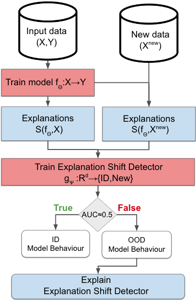
Figure 1: “Explanation Shift Detector” workflow diagram. The model $f_{\theta}$ is trained on $(X,Y)$, and outputs explanations for both distributions. Then the “Explanation Shift detector” $g_{\psi}$ receives the explanations and aims to predict if the model behaviour is different between them. If the $AUC\neq 0.5$ then there is a change in the data that implies a change in the model behaviour. Finally, we can proceed to account $g_{\psi}$ with explainable AI techniques and identify the roots of the change.

4 Mathematical Analysis

In this section, we provide a mathematical analysis on how changes in the distributions impact the explanation space and compare to the input data space and the prediction space.

4.1 Explanation vs Prediction spaces

This section exploits the benefits of the explanation space with respect to the prediction space when detecting distribution shifts. We will provide a theorem proving that OOD predictions imply OOD Explanations, and a counterexample for the opposite case, OOD Explanations do not necessarily imply OOD predictions.

Proposition 1.

Given a model $f_{\theta}:X\to Y$. If $f_{\theta}(x^{{}^{\prime}})\neq f_{\theta}(x)$, then $\mathcal{S}(f_{\theta},x^{{}^{\prime}})\neq\mathcal{S}(f_{\theta},x)$.

$$\texttt{Given}\quad f_{\theta}(x)\neq f_{\theta}(x^{\prime})$$ (5)

$$\sum_{j=1}^{p}\mathcal{S}_{j}(f_{\theta},x)=f_{\theta}(x)-E_{X}[f_{\theta}(X)]$$ (6)

$$\texttt{then}\quad\mathcal{S}(f,x)\ \neq\mathcal{S}(f,x^{\prime})$$ (7)

By additivity/efficiency property of the Shapley values (Aas et al., 2021) (equation (3)), if the prediction between two instances is different, then they differ in at least one component of their explanation vectors.

The opposite direction does not hold, we can have out-of-distributions explanations but in-distribution predictions, as we can see in the following counter-example:

Example 4.1 (Explanation shift that does not affect the prediction distribution).

Given $\mathcal{D}^{tr}$ is generated from $(X_{1},X_{2},Y),X_{1}\sim U(0,1),X_{2}\sim U(1,2),Y=X_{1}+X_{2}+\epsilon$ and thus the model is $f(x)=x_{1}+x_{2}$. If $\mathcal{D}^{new}$ is generated from $X_{1}^{new}\sim U(1,2),X_{2}^{new}\sim U(0,1)$, the prediction distributions are identical $f_{\theta}(\mathcal{D}^{tr}),f_{\theta}(\mathcal{D}^{new})\sim U(0,3)$, but explanation distributions are different $S(f_{\theta},\mathcal{D}^{tr}_{X})\neq S(f_{\theta},\mathcal{D}^{new})$

$$\forall i\in\{1,2\}\quad\mathcal{S}_{i}(f_{\theta},x)=\alpha_{i}\cdot x_{i}$$ (8)

$$\forall i\in\{1,2\}\Rightarrow\mathcal{S}_{i}(f_{\theta},X))\neq\mathcal{S}_{i}(f_{\theta},X^{new})$$ (9)

$$\Rightarrow f_{\theta}(X)=f_{\theta}(X^{new})$$ (10)

In this example, we can calculate the IID linear interventional Shapley values (Aas et al., 2021). Then the Shapley values for each feature will have different distributions between train and out-of-distribution explanations, but the prediction space will remain unaltered.

4.2 Explanation shifts vs input data distribution shifts

This section provides two different examples of situations where changes in the explanation space can correctly account for model behavior changes, but where statistical checks on the input data either (1) cannot detect changes, or (2) detect changes that do not affect model behavior. For simplicity the model used in the analytical examples is a linear regression where, if the features are independent, the Shapley value can be estimated by $\mathcal{S}(f_{\theta},x_{i})=a_{i}(x_{i}-\mu_{i})$, where $a_{i}$ are the coefficients of the linear model and $\mu_{i}$ the mean of the features (Chen et al., 2020).

4.2.1 Detecting multivariate shift

One type of distribution shift that is challenging to detect comprises cases where the univariate distributions for each feature $j$ are equal between the source $\mathcal{D}^{tr}$ and the unseen dataset $\mathcal{D}^{new}$, but where interdependencies among different features change. On the other hand, multi-covariance statistical testing is not an easy task that has high sensitivity easily leading to false positives. The following examples demonstrate that Shapley values account for co-variate interaction changes while a univariate statistical test will provide false negatives.
Example 1: Multivariate Shift
Let $X=(X_{1},X_{2})\sim{\tiny N\left(\begin{bmatrix}\mu_{1}\\ \mu_{2}\end{bmatrix},\begin{bmatrix}\sigma^{2}_{x_{1}}&0\\ 0&\sigma^{2}_{x_{2}}\end{bmatrix}\right),}$
$X^{new}=(X^{new}_{1},X^{new}_{2})\sim{\tiny N\left(\begin{bmatrix}\mu_{1}\\ \mu_{2}\end{bmatrix},\begin{bmatrix}\sigma^{2}_{x_{1}}&\rho\sigma_{x_{1}}\sigma_{x_{2}}\\ \rho\sigma_{x_{1}}\sigma_{x_{2}}&\sigma^{2}_{x_{2}}\end{bmatrix}\right)}$. We fit a linear model $f_{\theta}(X_{1},X_{2})=\gamma+a\cdot X_{1}+b\cdot X_{2}.\hskip 14.22636pt$ $X_{1}$ and $X_{2}$ are identically distributed with $X_{1}^{new}$ and $X_{2}^{new}$, respectively, while this does not hold for the corresponding SHAP values $\mathcal{S}_{j}(f_{\theta},X)$ and $\mathcal{S}_{j}(f_{\theta},X^{new})$.

The detailed analysis is given in the Appendix.

4.2.2 Shifts on uninformative features by the model

Another typical problem is false positives when a statistical test recognizes differences between a source distribution and a new distribution, though the differences do not affect the model behavior(Grinsztajn et al., 2022). One of the intrinsic properties that Shapley values satisfy is the “Dummy”, where a feature $j$ that does not change the predicted value, regardless of which coalition the feature is added, should have a Shapley value of $0$. If $\mathrm{val}(S\cup\{j\})=\mathrm{val}(S)$ for all $S\subseteq\{1,\ldots,p\}$ then $\mathcal{S}_{j}(f_{\theta},x_{i})=0$.

Example 2: Unused features Let $X=(X_{1},X_{2},X_{3})\sim N(\mu,\mathrm{diag}(c))$, and $X^{new}=(X^{new}_{1},X^{new}_{2},X^{new}_{3})\sim N(\mu,\mathrm{diag}(c^{\prime}))$, where $\mathrm{c}$ and $\mathrm{c^{\prime}}$ are an identity matrix of order three and $\mu=(\mu_{1},\mu_{2},\mu_{3})$. We now create a synthetic target $Y=a_{0}+a_{1}\cdot X_{1}+a_{2}\cdot X_{2}+\epsilon$ that is independent of $X_{3}$. We train a linear regression $f_{\theta}$ on $(X,Y)$, with coefficients $a_{0},a_{1},a_{2},a_{3}$. Then if $\mu_{3}^{\prime}\neq\mu_{3}$ or $c_{3}^{\prime}\neq c_{3}$, then $P(X_{3})$ can be different from $P(X_{3}^{new})$ but $\mathcal{S}_{3}(f_{\theta},X)=\mathcal{S}_{3}(f_{\theta},X^{new})$

5 Experiments

The first experimental section explores the detection of distribution shift on the previoust synthetic examples. The second part explores the utility of explanation shift on real data applications.

5.1 Explanation Shift Detection

5.1.1 Detecting multivariate shift

Given two bivariate normal distributions $X=(X_{1},X_{2})\sim N\left(0,\begin{bmatrix}1&0\\ 0&1\end{bmatrix}\right)$ and $X^{new}=(X^{new}_{1},X^{new}_{2})\sim N\left(0,\begin{bmatrix}1&0.2\\ 0.2&1\end{bmatrix}\right)$, then, for each feature $j$ the underlying distribution is equally distributed between $X$ and $X^{new}$, $\forall j\in\{1,2\}:P(X_{j})=P(X^{new}_{j})$, and what is different are the interaction terms between them. We now create a synthetic target $Y=X_{1}\cdot X_{2}+\epsilon$ with $\epsilon\sim N(0,0.1)$ and fit a gradient boosting decision tree $f_{\theta}(X)$. Then we compute the SHAP explanation values for $\mathcal{S}(f_{\theta},X)$ and $\mathcal{S}(f_{\theta},X^{new})$

Table 1: Displayed results are the one-tailed p-values of the Kolmogorov-Smirnov test comparison between two underlying distributions. Small p-values indicates that compared distributions would be very unlikely to be equally distributed. SHAP values correctly indicate the interaction changes that individual distribution comparisons cannot detect

Comparison	p-value	Conclusions
$P(X_{1})$, $P(X^{new}_{1})$	0.33	Not Distinct
$P(X_{2})$, $P(X^{new}_{2})$	0.60	Not Distinct
$\mathcal{S}_{1}(f_{\theta},X)$, $\mathcal{S}_{1}(f_{\theta},X^{new})$	$3.9\mathrm{e}{-153}$	Distinct
$\mathcal{S}_{2}(f_{\theta},X)$, $\mathcal{S}_{2}(f_{\theta},X^{new})$	$2.9\mathrm{e}{-148}$	Distinct

Having drawn $50,000$ samples from both $X$ and $X^{new}$, in Table 1, we evaluate whether changes on the input data distribution or on the explanations are able to detect changes on covariate distribution. For this, we compare the one-tailed p-values of the Kolmogorov-Smirnov test between the input data distribution, and the explanations space. Explanation shift correctly detects the multivariate distribution change that univariate statistical testing can not detect.

5.1.2 Uninformative features on synthetic data

To have an applied use case of the synthetic example from the methodology section, we create a three-variate normal distribution $X=(X_{1},X_{2},X_{3})\sim N(0,I_{3})$, where $I_{3}$ is an identity matrix of order three. The target variable is generated $Y=X_{1}\cdot X_{2}+\epsilon$ being independent of $X_{3}$. For both, training and test data, $50,000$ samples are drawn. Then out-of-distribution data is created by shifting $X_{3}$, which is independent of the target, on test data $X^{new}_{3}=X^{te}_{3}+1$.

Table 2: Distribution comparison when modifying a random noise variable on test data. The input data shifts while explanations and predictions do not.

Comparison	Conclusions
$P(X^{te}_{3})$, $P(X^{new}_{3})$	Distinct
$f_{\theta}(X^{te})$, $f_{\theta}(X^{new})$	Not Distinct
$\mathcal{S}(f_{\theta},X^{te})$, $\mathcal{S}(f_{\theta},X^{new})$	Not Distinct

In Table 2, we see how an unused feature has changed the input distribution, but the explanation space and performance evaluation metrics remain the same. The “Distinct/Not Distinct” conclusion is based on the one-tailed p-value of the Kolmogorov-Smirnov test drawn out of $50,000$ samples for both distributions.

5.1.3 Explanation shift that does not affect the prediction

In this case we provide a situation when we have changes in the input data distributions that affect the model explanations but do not affect the model predictions due to positive and negative associations between the model predictions and the distributions cancel out producing a vanishing correlation in the mixture of the distribution (Yule’s effect 4.1).

We create a train and test data by drawing $50,000$ samples from a bi-uniform distribution $X_{1}\sim U(0,1),\quad X_{2}\sim U(1,2)$ the target variable is generated by $Y=X_{1}+X_{2}$ where we train our model $f_{\theta}$. Then if out-of-distribution data is sampled from $X_{1}^{new}\sim U(1,2)$, $X_{2}^{new}\sim U(0,1)$

Table 3: Distribution comparison over how the change on the contributions of each feature can cancel out to produce an equal prediction (cf. Section 4.1), while explanation shift will detect this behaviour changes on the predictions will not.

Comparison	Conclusions
$f(X^{te})$, $f(X^{new})$	Not Distinct
$\mathcal{S}(f_{\theta},X^{te}_{2})$, $\mathcal{S}(f_{\theta},X^{new}_{2})$	Distinct
$\mathcal{S}(f_{\theta},X^{te}_{1})$, $\mathcal{S}(f_{\theta},X^{new}_{1})$	Distinct

In Table 3, we see how an unused feature has changed the input distribution, but the explanation space and performance evaluation metrics remain the same. The “Distinct/Not Distinct” conclusion is based on the one-tailed p-value of the Kolmogorov-Smirnov test drawn out of $50,000$ samples for both distributions.

5.2 Explanation Shift Detector: Measurements on synthetic data

In this work, we are proposing explanation shifts as an indicator of out-of-distribution model behavior. The Explanation Shift Detector (cf. Section 3.2), aims to detect if the behaviour of a machine learning model is different between unseen data and training data.

As ablation studies, in this work, we compare our method that learns on the explanations space (eq. 4) against learning on different spaces: on input data space, that detects out-of-distribution data, but is independent of the model:

$$\phi=\operatorname*{arg\,min}_{\tilde{\phi}}\sum_{x\in X\cup X^{new}}\ell(g_{\tilde{\phi}}({\color[rgb]{0,0,1}x})),a_{x})$$ (11)

on output space, that detects out-of-distribution predictions, but can suffer from Yule’s effect of distribution shift (cf. section 4.1):

$$\Upsilon=\operatorname*{arg\,min}_{\tilde{\Upsilon}}\sum_{x\in X\cup X^{new}}\ell(g_{\tilde{\Upsilon}}({\color[rgb]{0,0,1}f_{\theta}(x)}),a_{x})$$ (12)

Our first experiment showcases the two main contributions of our method: $(i)$ being more sensitive than output spaces and input spaces to changes in the model behaviour and, $(ii)$ accounting for its drivers.

In order to do this, we first generate a synthetic dataset with a shift similar to the multivariate shift one (cf. Section 5.1.1), but we add an extra variable $X_{3}=N(0,1)$ and generate our target $Y=X_{1}\cdot X_{2}+X_{3}$, and parametrize the multivariate shift between $\rho=r(X_{1},X_{2})$. For the model $f_{\theta}$ we use a gradient boosting decision tree, while for $g_{\psi}$ we use a logistic regression. For model performance metrics, as we are in binary classification scenarios, we use the Area Under the Curve (AUC)—a metric that illustrates the diagnostic ability of a binary classifier system as its discrimination threshold is varied (Hastie et al., 2001).

Table 4: Conceptual comparison table over different detection methods over the examples discussed above. The “Explanation Shift Detector”, learning $g_{\psi}$ over the explanation space is the only method that achieves the desired results and is accountable. We evaluate accountability by checking if the feature attributions of the detection method correspond with the synthetic shift generated in both scenarios

Detection Method	Multiv.	Uninf.	Accountability
Explanation sp. ($g_{\psi}$)	✓	✓	✓
Input space($g_{\phi}$)	✓	✗	✗
Prediction sp.($g_{\Upsilon}$)	✓	✓	✗
Input Shift(Univ)	✗	✗	✗
Input Shift(Mult.)	✓	✗	✗
Output Shift	✓	✓	✗
Uncertainty	$\sim$	✓	✓

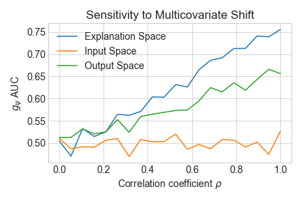
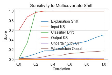
Figure 2: In the left figure, comparison of the performance of Explanation Shift Detector, based on learning on different spaces. Learning on the explanation space shows more sensitivity than learning in the output space. In the right figure, related work comparison of SOTA methods (Van Looveren et al., 2019; Mougan & Nielsen, 2023; Rabanser et al., 2019), good indicators should follow a progressive steady positive slope.

In Table 4 and Figure 2, we show the effectos of our algorithmic approach when learning on different spaces. In the sensitivity experiment, we see that the Explanation Space offers a higher sensitivity towards distribution shift detection. This can be explained using the additive property of the Shapley values. What the explanation space is representing is a higher dimensional space than the output space that contains the model behavior. On the other hand, the input space, even if it has the same dimensional, it does not contain the projection of the model behaviour. Furthermore, we can proceed and explain what are the reasons driving the drift, by extracting the coefficients of $g_{\psi}$ of the $\rho=1$ case, $\beta_{1}\neq 0,\beta_{2}\neq 0,\beta_{3}\sim 0$, providing global explainability about the features that are shifting, the Explanation Shift Detector correctly detects the features that are causing the drift.

In the right image of Figure 2 the comparison against other state-of-the-art techniques: statistical differences on the input data (Input KS, Classifier Drift) (Van Looveren et al., 2019; Diethe et al., 2019), that are independent of the model; uncertainty estimation  (Kim et al., 2020; Mougan & Nielsen, 2023; Romano et al., 2021), whose properties under specific types of shift remains unknown, or statistical changes on the output data (Fort et al., 2021; Garg et al., 2020) (K-S and Wasserstein Distance), which correctly detect that the model behaviour is changing, but lacks the sensitivity of the explanation space.

5.3 Experiments on real data: Inspecting out-of-distribution explanations

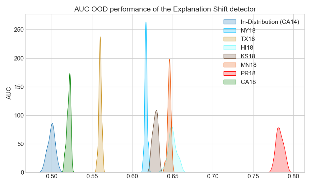
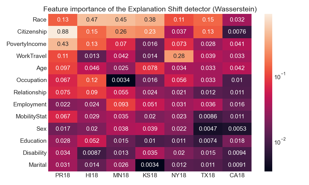
Figure 3: In the left figure, comparison of the performance of Explanation Shift Detector, in different states. Learning in the explanation space shows more sensitivity than learning in the output space. In the right figure, strength analysis of features driving the change in model behaviour.

The need for explainable model monitoring has been expressed by several authors (Klaise et al., 2020; Diethe et al., 2019; Mougan et al., 2021; Budhathoki et al., 2021), understanding the effects of the distribution shift on the behaviour can provide algorithmic transparency to stakeholders and to the ML engineering team.

After providing analytical examples and experiments with synthetic data, still there is the challenge of operationalizing the Explanation Shift Detector to real-world data. In this section, we provide experiments on the ACSTravelTime task, whose goal is to predict whether an individual has a commute to work that is longer than 20 minutes. To create the distribution shift we train the model $f_{\theta}$ in California in 2014 and evaluating in the rest of the states in 2018, creating a geopolitical and temporal shift. The model $g_{\theta}$ is trained each time on each state using only the $X^{new}$ in the absence of the label, and its performance is evaluated by a 50/50 random train-test split. As models we use a gradient boosting decision tree(Chen & Guestrin, 2016; Prokhorenkova et al., 2018) as estimator $f_{\theta}$, approximating the Shapley values by TreeExplainer (Lundberg et al., 2020), and using logistic regression for the Explanation Shift Detector.

Our hypothesis is that the AUC in OOD data of the “Explanation Shift Detector” $g_{\psi}$ will be higher than ID data due to OOD model behaviour. In Figure 3, we can see the performance of the “Explanation Shift Detector” over different data distributions. The baseline is a hold-out set of $ID-CA14$, and the closest AUC is for $CA18$, where there is just a temporal shift, then the OOD detection performance over the rest of states. The most OOD state is Puerto Rico (PR18).

The next question that we aim to answer is what are the features where the model behaviour is different. For this, we do a distribution comparison between the linear coefficients of the “Explanation Shift Detector” in ID and in OOD. As a distance measure, we use the Wasserstein distance between 1000 in-distribution bootstraps using a $63.2\%$ sampling fraction (Hastie et al., 2001) from California-14 and 1000 OOD bootstraps from other states in 2018 (see 3). In the right image 3, for PR18, we see that the most important feature is the citizenship status.

We also perform an across-task evaluation, by comparing it with the other prediction task in the appendix. We can see how, even if some of the features are in present in different prediction tasks, the weight and importance order assigned by the “Explanation Shift Detector” is different. One of the main contributions of this method is that is not just how distribution differs, but how they differ with respect to the model.

6 Discussion

In this work, we have proposed explanation shifts as a key indicator for investigating the interaction between distribution shifts and the learned model. Finding that monitoring explanations shift is a better indicator than model varying behaviour.

Our approach is not able to detect concept shifts, as concept shift requires understanding the interaction between prediction and response variables. By the very nature of concept shifts, such changes can only be understood if new data comes with labeled responses. We work under the assumption that such labels are not available for new data and, therefore, our method is not able to predict the degradation of prediction performance under distribution shifts. All papers such as (Garg et al., 2021b; Mougan & Nielsen, 2023; Baek et al., 2022; Chen et al., 2022b; Fang et al., 2022; Baek et al., 2022; Miller et al., 2021) that address the monitoring of prediction performance have the same limitation. Only under specific assumptions, e.g., no occurrence of concept shift, performance degradation can be predicted with reasonable reliability.

The potential utility of explanation shifts as distribution shift indicators that affect the model in computer vision or natural language processing tasks remains an open question. We have used Shapley values to derive indications of explanation shifts, but we believe that other AI explanation techniques may be applicable and come with their own advantages.

7 Conclusions

Traditionally, the problem of detecting model shift behaviour has relied on measurements for detecting shifts in the input or output data distributions. In this paper, we have provided theoretical and experimental evidence that explanation shift can be a more suitable indicator to detect and identify the shift in the behaviour of machine learning models. We have provided mathematical analysis examples, synthetic data, and real data experimental evaluation. We found that measures of explanation shift can provide more insights than measures of the input distribution and prediction shift when monitoring machine learning models.

Reproducibility Statement

To ensure reproducibility, we make the data, code repositories, and experiments publicly available . Also, an open source Python package is released with the methods used (to be released upon acceptance). For our experiments, we used default scikit-learn parameters (Pedregosa et al., 2011). We describe the system requirements and software dependencies of our experiments. Experiments were run on a 4 vCPU server with 32 GB RAM.

Appendix A Analytical examples

This section covers the analytical examples demonstrations presented in the Section 4.2 of the main body of the paper.

A.1 Explanation vs Prediction

Proposition 2.

Given a model $f_{\theta}:X\to Y$. If $f_{\theta}(x^{{}^{\prime}})\neq f_{\theta}(x)$, then $\mathcal{S}(f_{\theta},x^{{}^{\prime}})\neq\mathcal{S}(f_{\theta},x)$.

$$\texttt{Given}\quad f_{\theta}(x)\neq f_{\theta}(x^{\prime})$$ (13)

$$\sum_{j=1}^{p}\mathcal{S}_{j}(f_{\theta},x)=f_{\theta}(x)-E_{X}[f_{\theta}(X)]$$ (14)

$$\texttt{then}\quad\mathcal{S}(f,x)\ \neq\mathcal{S}(f,x^{\prime})$$ (15)

Example A.1 (Explanation shift that does not affect the prediction distribution).

Given $\mathcal{D}^{tr}$ is generated from $(X_{1},X_{2},Y),X_{1}\sim U(0,1),X_{2}\sim U(1,2),Y=X_{1}+X_{2}+\epsilon$ and thus the model is $f(x)=x_{1}+x_{2}$. If $\mathcal{D}^{new}$ is generated from $X_{1}^{new}\sim U(1,2),X_{2}^{new}\sim U(0,1)$, the prediction distributions are identical $f_{\theta}(\mathcal{D}^{tr}),f_{\theta}(\mathcal{D}^{new})\sim U(0,3)$, but explanation distributions are different $S(f_{\theta},\mathcal{D}^{tr}_{X})\neq S(f_{\theta},\mathcal{D}^{new})$

$$\forall i\in\{1,2\}\quad\mathcal{S}_{i}(f_{\theta},x)=\alpha_{i}\cdot x_{i}$$ (16)

$$\forall i\in\{1,2\}\Rightarrow\mathcal{S}_{i}(f_{\theta},X))\neq\mathcal{S}_{i}(f_{\theta},X^{new})$$ (17)

$$\Rightarrow f_{\theta}(X)=f_{\theta}(X^{new})$$ (18)

A.2 Explanation shifts vs input data distribution shifts

A.2.1 Multivariate shift

Example 1: Multivariate Shift Let $X=(X_{1},X_{2})\sim N\left(\begin{bmatrix}\mu_{1}\\ \mu_{2}\end{bmatrix},\begin{bmatrix}\sigma^{2}_{x_{1}}&0\\ 0&\sigma^{2}_{x_{2}}\end{bmatrix}\right)$ and $X^{ood}=(X^{ood}_{1},X^{ood}_{2})\sim N\left(\begin{bmatrix}\mu_{1}\\ \mu_{2}\end{bmatrix},\begin{bmatrix}\sigma^{2}_{x_{1}}&\rho\sigma_{x_{1}}\sigma_{x_{2}}\\ \rho\sigma_{x_{1}}\sigma_{x_{2}}&\sigma^{2}_{x_{2}}\end{bmatrix}\right)$ and target $Y=X_{1}+X_{2}+\epsilon$. We fit a linear model $f_{\theta}(X_{1},X_{2})=\gamma+a\cdot X_{1}+b\cdot X_{2}.\hskip 14.22636pt$ $X_{1}$ and $X_{2}$ are identically distributed with $X_{1}^{ood}$ and $X_{2}^{ood}$, respectively, while this does not hold for the corresponding SHAP values $\mathcal{S}_{j}(f_{\theta},X)$ and $\mathcal{S}_{j}(f_{\theta},X^{ood})$.

$$\mathcal{S}_{1}(f_{\theta},x)=a(x_{1}-\mu_{1})$$ (19)

$$\mathcal{S}_{1}(f_{\theta},x^{ood})=$$ (20)

$$=\frac{1}{2}[\mathrm{val}(\{1,2\})-\mathrm{val}(\{2\})]+\frac{1}{2}[\mathrm{val}(\{1\})-\mathrm{val}(\emptyset)]$$ (21)

$$\mathrm{val}(\{1,2\})=E[f_{\theta}|X_{1}=x_{1},X_{2}=x_{2}]=ax_{1}+bx_{2}$$ (22)

$$\mathrm{val}(\emptyset)=E[f_{\theta}]=a\mu_{1}+b\mu_{2}$$ (23)

$$\mathrm{val}(\{1\})=E[f_{\theta}(x)|X_{1}=x_{1}]+b\mu_{2}$$ (24)

$$\mathrm{val}(\{1\})=\mu_{1}+\rho\frac{\rho_{x_{1}}}{\sigma_{x_{2}}}(x_{1}-\sigma_{1})+b\mu_{2}$$ (25)

$$\mathrm{val}(\{2\})=\mu_{2}+\rho\frac{\sigma_{x_{2}}}{\sigma_{x_{1}}}(x_{2}-\mu_{2})+a\mu_{1}$$ (26)

$$\Rightarrow\mathcal{S}_{1}(f_{\theta},x^{ood})\neq a(x_{1}-\mu_{1})$$ (27)

A.2.2 Uninformative Features

Example 2: Unused features Let $X=(X_{1},X_{2},X_{3})\sim N(\mu,\mathrm{diag}(c))$, and $X^{ood}=(X^{ood}_{1},X^{ood}_{2},X^{ood}_{3})\sim N(\mu,\mathrm{diag}(c^{\prime}))$, where $\mathrm{c}$ and $\mathrm{c^{\prime}}$ are an identity matrix of order three and $\mu=(\mu_{1},\mu_{2},\mu_{3})$. We now create a synthetic target $Y=a_{0}+a_{1}\cdot X_{1}+a_{2}\cdot X_{2}+\epsilon$ that is independent of $X_{3}$. We train a linear regression $f_{\theta}$ on $(X,Y)$, with coefficients $a_{0},a_{1},a_{2},a_{3}$. Then if $\mu_{3}^{\prime}\neq\mu_{3}$ or $c_{3}^{\prime}\neq c_{3}$, then $P(X_{3})$ can be different from $P(X_{3}^{ood})$ but $\mathcal{S}_{3}(f_{\theta},X)=\mathcal{S}_{3}(f_{\theta},X^{ood})$

$$X_{3}\sim N(\mu_{3},c_{3}),X_{3}^{ood}\sim N(\mu_{3}^{{}^{\prime}},c_{3}^{{}^{\prime}})$$ (28)

$$\mathrm{If}\quad\mu_{3}^{{}^{\prime}}\neq\mu_{3}\quad\mathrm{or}\quad c_{3}^{{}^{\prime}}\neq c_{3}\rightarrow P(X_{3})\neq P(X_{3}^{ood})$$ (29)

$$\mathcal{S}(f_{\theta},X)=\left(\begin{bmatrix}a_{1}(X_{1}-\mu_{1})\\ a_{2}(X_{2}-\mu_{2})\\ a_{3}(X_{3}-\mu_{3})\end{bmatrix}\right)=\left(\begin{bmatrix}a_{1}(X_{1}-\mu_{1})\\ a_{2}(X_{2}-\mu_{2})\\ 0\end{bmatrix}\right)$$ (30)

$$\mathcal{S}_{3}(f_{\theta},X)=\mathcal{S}_{3}(f_{\theta},X^{ood})$$ (31)

Appendix B Experiments on real data

In this section, we extend the prediction task of the main body of the paper. The methodology used follows the same structure, we start by creating a distribution shift by training the model $f_{\theta}$ in California in 2014 and evaluating it in the rest of the states in 2018, creating a geopolitical and temporal shift. The model $g_{\theta}$ is trained each time on each state using only the $X^{ood}$ in the absence of the label, and its performance is evaluated by a 50/50 random train-test split. As models we use a gradient boosting decision tree(Chen & Guestrin, 2016; Prokhorenkova et al., 2018) as estimator $f_{\theta}$, approximating the Shapley values by TreeExplainer (Lundberg et al., 2020), and using logistic regression for the Explanation Shift Detector.

B.1 ACS Employment

The goal of this task is to predict whether an individual, between the ages of 16 and 90, is employed. For this prediction task the AUC of all the other states (except PR18) falls below $0.60$, indicating not high OOD explanations. For the most OOD state, PR18, the “Explanation Shift Detector” finds that the model has shifted due to features such as Citizenship or Military Service.

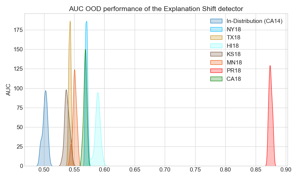
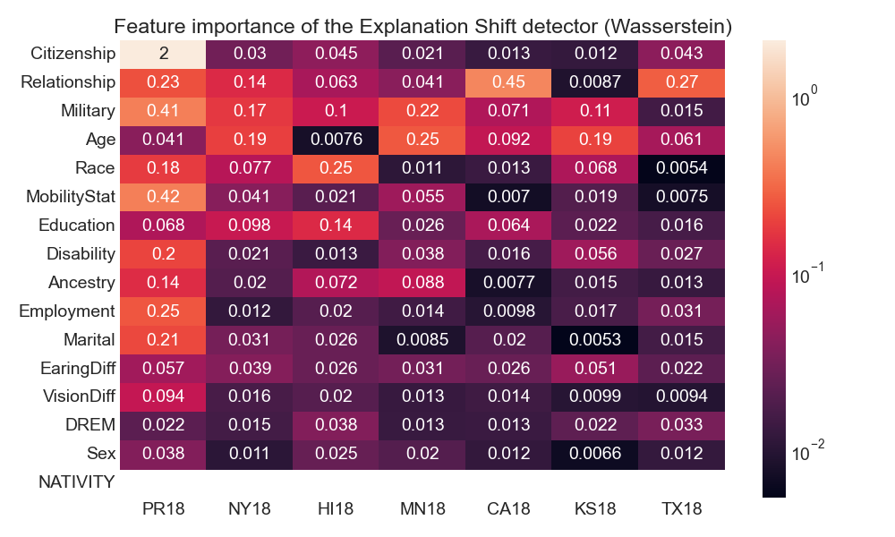
Figure 4: In the left figure, comparison of the performance of Explanation Shift Detector, in different states for the ACS Employment dataset. For this dataset, most of the states have the same OOD detection AUC, except for PR18. This difference in the model behaviour is due to features such as Citizenship and Military Service. Features such as difficulties in hearing or seeing, do not play a role in the OOD model behaviour.

B.2 ACS Income

The goal of this task is to predict whether an individual’s income is above $\$50,000$, only includes individuals above the age of 16, and report an income of at least $\$100$. This dataset can serve as a comparable replacement to the UCI Adult dataset.

For this prediction task the results are different from the previous two cases, the state with the highest OOD score is $KS18$, with the “Explanation Shift Detector” highlighting features as Place of Birth, Race or Working Hours Per Week. The closest state to ID is CA18, where there is only a temporal shift without any geospatial distribution shift.

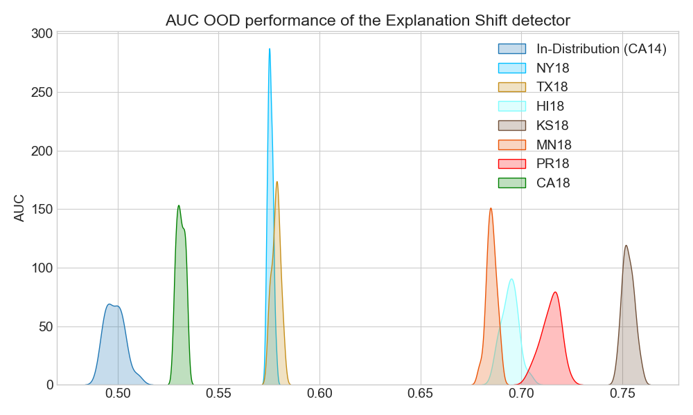
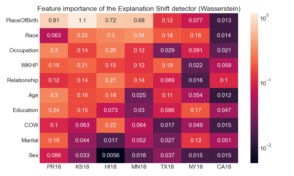
Figure 5: In the left figure, comparison of the performance of Explanation Shift Detector, in different states for the ACS Income prediction task. In the left figure, we can see how the state with the highest OOD AUC detection is KS18 and not PR18 as in other prediction tasks, this difference with respect to the other prediction task can be attributed to “Place of Birth”, whose feature attributions the model finds to be more different than in CA14.

B.3 ACS Mobility

The goal of this task is to predict whether an individual had the same residential address one year ago, only including individuals between the ages of 18 and 35. The goal of this filtering is to increase the prediction task difficulty, staying at the same address base rate is above $90\%$ for the population (Ding et al., 2021).

The results of this experiment present a similar behaviour as the ACS Income prediction task (cf. Section 5), where the in-land states of the US are in an AUC range of $0.55-0.70$ and is the state of PR18 who achieves a higher OOD AUC. The features driving this behaviour are Citizenship for PR18 and Ancestry(Census record of your ancestors’ lives with details like where they lived, who they lived with, and what they did for a living) for the other states.

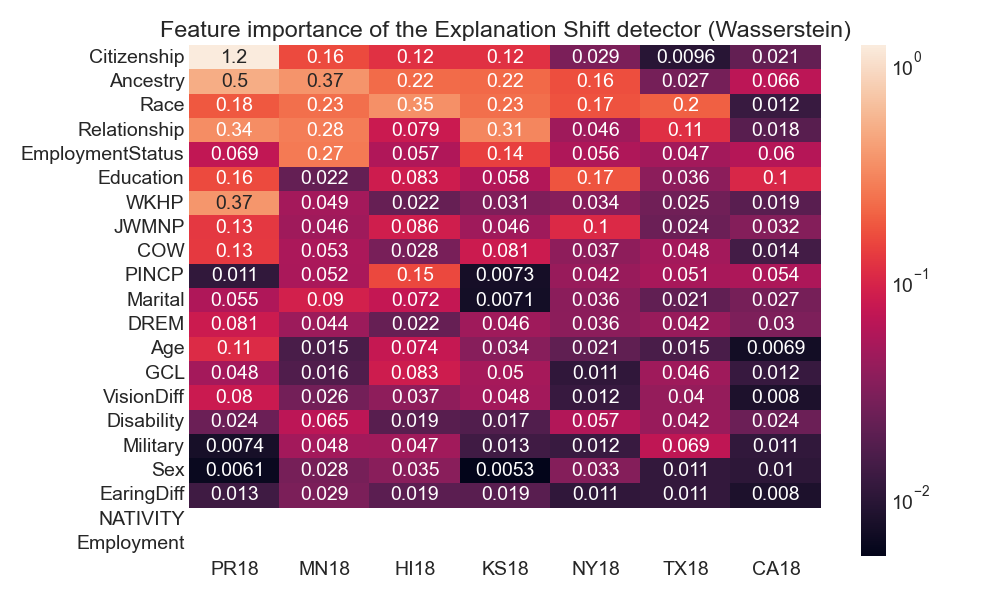
Figure 6: In the left figure, comparison of the performance of Explanation Shift Detector, in different states for the ACS Mobility dataset. Except for PR18, all the other states fall below an AUC of OOD detection of $0.70$. If we look at the features driving this difference is due to the Citizenship and the Ancestry relationship. For the other states protected social attributes such as Race or Marital status play an important role.

References

- Aas et al. (2021) Aas, K., Jullum, M., and Løland, A. Explaining individual predictions when features are dependent: More accurate approximations to shapley values. Artif. Intell., 298:103502, 2021. doi: 10.1016/j.artint.2021.103502. URL https://doi.org/10.1016/j.artint.2021.103502.
- Arrieta et al. (2020) Arrieta, A. B., Rodríguez, N. D., Ser, J. D., Bennetot, A., Tabik, S., Barbado, A., García, S., Gil-Lopez, S., Molina, D., Benjamins, R., Chatila, R., and Herrera, F. Explainable artificial intelligence (XAI): concepts, taxonomies, opportunities and challenges toward responsible AI. Inf. Fusion, 58:82–115, 2020. doi: 10.1016/j.inffus.2019.12.012. URL https://doi.org/10.1016/j.inffus.2019.12.012.
- Aumann & Dreze (1974) Aumann, R. J. and Dreze, J. H. Cooperative games with coalition structures. International Journal of game theory, 3(4):217–237, 1974.
- Baek et al. (2022) Baek, C., Jiang, Y., Raghunathan, A., and Kolter, J. Z. Agreement-on-the-line: Predicting the performance of neural networks under distribution shift. In Oh, A. H., Agarwal, A., Belgrave, D., and Cho, K. (eds.), Advances in Neural Information Processing Systems, 2022. URL https://openreview.net/forum?id=EZZsnke1kt.
- Balestra et al. (2022) Balestra, C., Li, B., and Müller, E. Enabling the visualization of distributional shift using shapley values. In NeurIPS 2022 Workshop on Distribution Shifts: Connecting Methods and Applications, 2022. URL https://openreview.net/forum?id=HxnGNo2ADT.
- Barredo Arrieta et al. (2020) Barredo Arrieta, A., Díaz-Rodríguez, N., Del Ser, J., Bennetot, A., Tabik, S., Barbado, A., Garcia, S., Gil-Lopez, S., Molina, D., Benjamins, R., Chatila, R., and Herrera, F. Explainable artificial intelligence (xai): Concepts, taxonomies, opportunities and challenges toward responsible ai. Information Fusion, 58:82–115, 2020. ISSN 1566-2535. doi: https://doi.org/10.1016/j.inffus.2019.12.012. URL https://www.sciencedirect.com/science/article/pii/S1566253519308103.
- Borisov et al. (2021) Borisov, V., Leemann, T., Seßler, K., Haug, J., Pawelczyk, M., and Kasneci, G. Deep neural networks and tabular data: A survey, 2021. URL https://arxiv.org/abs/2110.01889.
- Budhathoki et al. (2021) Budhathoki, K., Janzing, D., Blöbaum, P., and Ng, H. Why did the distribution change? In Banerjee, A. and Fukumizu, K. (eds.), The 24th International Conference on Artificial Intelligence and Statistics, AISTATS 2021, April 13-15, 2021, Virtual Event, volume 130 of Proceedings of Machine Learning Research, pp. 1666–1674. PMLR, 2021. URL http://proceedings.mlr.press/v130/budhathoki21a.html.
- Chen et al. (2020) Chen, H., Janizek, J. D., Lundberg, S. M., and Lee, S. True to the model or true to the data? CoRR, abs/2006.16234, 2020. URL https://arxiv.org/abs/2006.16234.
- Chen et al. (2022a) Chen, H., Covert, I. C., Lundberg, S. M., and Lee, S. Algorithms to estimate shapley value feature attributions. CoRR, abs/2207.07605, 2022a. doi: 10.48550/arXiv.2207.07605. URL https://doi.org/10.48550/arXiv.2207.07605.
- Chen et al. (2022b) Chen, L., Zaharia, M., and Zou, J. Y. Estimating and explaining model performance when both covariates and labels shift. In Oh, A. H., Agarwal, A., Belgrave, D., and Cho, K. (eds.), Advances in Neural Information Processing Systems, 2022b. URL https://openreview.net/forum?id=BK0O0xLntFM.
- Chen & Guestrin (2016) Chen, T. and Guestrin, C. XGBoost: A scalable tree boosting system. In Proceedings of the 22nd ACM SIGKDD International Conference on Knowledge Discovery and Data Mining, KDD ’16, pp. 785–794, New York, NY, USA, 2016. ACM. ISBN 978-1-4503-4232-2. doi: 10.1145/2939672.2939785. URL http://doi.acm.org/10.1145/2939672.2939785.
- Diethe et al. (2019) Diethe, T., Borchert, T., Thereska, E., Balle, B., and Lawrence, N. Continual learning in practice. ArXiv preprint, https://arxiv.org/abs/1903.05202, 2019.
- Ding et al. (2021) Ding, F., Hardt, M., Miller, J., and Schmidt, L. Retiring adult: New datasets for fair machine learning. In Ranzato, M., Beygelzimer, A., Dauphin, Y. N., Liang, P., and Vaughan, J. W. (eds.), Advances in Neural Information Processing Systems 34: Annual Conference on Neural Information Processing Systems 2021, NeurIPS 2021, December 6-14, 2021, virtual, pp. 6478–6490, 2021. URL https://proceedings.neurips.cc/paper/2021/hash/32e54441e6382a7fbacbbbaf3c450059-Abstract.html.
- Elsayed et al. (2021) Elsayed, S., Thyssens, D., Rashed, A., Schmidt-Thieme, L., and Jomaa, H. S. Do we really need deep learning models for time series forecasting? CoRR, abs/2101.02118, 2021. URL https://arxiv.org/abs/2101.02118.
- Fang et al. (2022) Fang, Z., Li, Y., Lu, J., Dong, J., Han, B., and Liu, F. Is out-of-distribution detection learnable? In Oh, A. H., Agarwal, A., Belgrave, D., and Cho, K. (eds.), Advances in Neural Information Processing Systems, 2022. URL https://openreview.net/forum?id=sde_7ZzGXOE.
- Fort et al. (2021) Fort, S., Ren, J., and Lakshminarayanan, B. Exploring the limits of out-of-distribution detection. Advances in Neural Information Processing Systems, 34, 2021. URL https://arxiv.org/abs/2106.03004.
- Frye et al. (2020) Frye, C., Rowat, C., and Feige, I. Asymmetric shapley values: incorporating causal knowledge into model-agnostic explainability. In Larochelle, H., Ranzato, M., Hadsell, R., Balcan, M., and Lin, H. (eds.), Advances in Neural Information Processing Systems 33: Annual Conference on Neural Information Processing Systems 2020, NeurIPS 2020, December 6-12, 2020, virtual, 2020. URL https://proceedings.neurips.cc/paper/2020/hash/0d770c496aa3da6d2c3f2bd19e7b9d6b-Abstract.html.
- Garg et al. (2020) Garg, S., Wu, Y., Balakrishnan, S., and Lipton, Z. A unified view of label shift estimation. In Larochelle, H., Ranzato, M., Hadsell, R., Balcan, M. F., and Lin, H. (eds.), Advances in Neural Information Processing Systems, volume 33, pp. 3290–3300. Curran Associates, Inc., 2020. URL https://proceedings.neurips.cc/paper/2020/file/219e052492f4008818b8adb6366c7ed6-Paper.pdf.
- Garg et al. (2021a) Garg, S., Balakrishnan, S., Kolter, Z., and Lipton, Z. Ratt: Leveraging unlabeled data to guarantee generalization. In International Conference on Machine Learning, pp. 3598–3609. PMLR, 2021a.
- Garg et al. (2021b) Garg, S., Balakrishnan, S., Lipton, Z. C., Neyshabur, B., and Sedghi, H. Leveraging unlabeled data to predict out-of-distribution performance. In NeurIPS 2021 Workshop on Distribution Shifts: Connecting Methods and Applications, 2021b.
- Grinsztajn et al. (2022) Grinsztajn, L., Oyallon, E., and Varoquaux, G. Why do tree-based models still outperform deep learning on typical tabular data? In Thirty-sixth Conference on Neural Information Processing Systems Datasets and Benchmarks Track, 2022. URL https://openreview.net/forum?id=Fp7__phQszn.
- Guerin et al. (2022) Guerin, J., Delmas, K., Ferreira, R. S., and Guiochet, J. Out-of-distribution detection is not all you need. In NeurIPS ML Safety Workshop, 2022. URL https://openreview.net/forum?id=hxFth8JGGR4.
- Guidotti et al. (2018) Guidotti, R., Monreale, A., Ruggieri, S., Turini, F., Giannotti, F., and Pedreschi, D. A survey of methods for explaining black box models. ACM Comput. Surv., 51(5), August 2018. ISSN 0360-0300.
- Hastie et al. (2001) Hastie, T., Tibshirani, R., and Friedman, J. The Elements of Statistical Learning. Springer Series in Statistics. Springer New York Inc., New York, NY, USA, 2001.
- Hendrycks & Gimpel (2017) Hendrycks, D. and Gimpel, K. A baseline for detecting misclassified and out-of-distribution examples in neural networks. In 5th International Conference on Learning Representations, ICLR 2017, Toulon, France, April 24-26, 2017, Conference Track Proceedings. OpenReview.net, 2017. URL https://openreview.net/forum?id=Hkg4TI9xl.
- Huang et al. (2021) Huang, R., Geng, A., and Li, Y. On the importance of gradients for detecting distributional shifts in the wild. Advances in Neural Information Processing Systems 34: Annual Conference on Neural Information Processing Systems 2021, NeurIPS 2021, abs/2110.00218, 2021. URL https://arxiv.org/abs/2110.00218.
- Huyen (2022) Huyen, C. Designing Machine Learning Systems: An Iterative Process for Production-Ready Applications. O’Reilly, 2022. URL ISBN-13:978-1098107963.
- Kenthapadi et al. (2022) Kenthapadi, K., Lakkaraju, H., Natarajan, P., and Sameki, M. Model monitoring in practice: Lessons learned and open challenges. In Proceedings of the 28th ACM SIGKDD Conference on Knowledge Discovery and Data Mining, KDD ’22, pp. 4800–4801, New York, NY, USA, 2022. Association for Computing Machinery. ISBN 9781450393850. doi: 10.1145/3534678.3542617. URL https://doi.org/10.1145/3534678.3542617.
- Kim et al. (2020) Kim, B., Xu, C., and Barber, R. F. Predictive inference is free with the jackknife+-after-bootstrap. In Larochelle, H., Ranzato, M., Hadsell, R., Balcan, M., and Lin, H. (eds.), Advances in Neural Information Processing Systems 33: Annual Conference on Neural Information Processing Systems 2020, NeurIPS 2020, December 6-12, 2020, virtual, 2020. URL https://proceedings.neurips.cc/paper/2020/hash/2b346a0aa375a07f5a90a344a61416c4-Abstract.html.
- Klaise et al. (2020) Klaise, J., Van Looveren, A., Cox, C., Vacanti, G., and Coca, A. Monitoring and explainability of models in production, 2020. URL https://arxiv.org/abs/2007.06299.
- Labs (2021) Labs, C. F. Inferring concept drift without labeled data. https://concept-drift.fastforwardlabs.com/, 2021.
- Lee et al. (2018) Lee, K., Lee, K., Lee, H., and Shin, J. A simple unified framework for detecting out-of-distribution samples and adversarial attacks. In Bengio, S., Wallach, H. M., Larochelle, H., Grauman, K., Cesa-Bianchi, N., and Garnett, R. (eds.), Advances in Neural Information Processing Systems 31: Annual Conference on Neural Information Processing Systems 2018, NeurIPS 2018, December 3-8, 2018, Montréal, Canada, pp. 7167–7177, 2018. URL https://proceedings.neurips.cc/paper/2018/hash/abdeb6f575ac5c6676b747bca8d09cc2-Abstract.html.
- Liu et al. (2020) Liu, W., Wang, X., Owens, J. D., and Li, Y. Energy-based out-of-distribution detection. In Larochelle, H., Ranzato, M., Hadsell, R., Balcan, M., and Lin, H. (eds.), Advances in Neural Information Processing Systems 33: Annual Conference on Neural Information Processing Systems 2020, NeurIPS 2020, December 6-12, 2020, virtual, 2020. URL https://proceedings.neurips.cc/paper/2020/hash/f5496252609c43eb8a3d147ab9b9c006-Abstract.html.
- Lundberg & Lee (2017) Lundberg, S. M. and Lee, S. A unified approach to interpreting model predictions. In Guyon, I., von Luxburg, U., Bengio, S., Wallach, H. M., Fergus, R., Vishwanathan, S. V. N., and Garnett, R. (eds.), Advances in Neural Information Processing Systems 30: Annual Conference on Neural Information Processing Systems 2017, December 4-9, 2017, Long Beach, CA, USA, pp. 4765–4774, 2017. URL https://proceedings.neurips.cc/paper/2017/hash/8a20a8621978632d76c43dfd28b67767-Abstract.html.
- Lundberg et al. (2020) Lundberg, S. M., Erion, G., Chen, H., DeGrave, A., Prutkin, J. M., Nair, B., Katz, R., Himmelfarb, J., Bansal, N., and Lee, S.-I. From local explanations to global understanding with explainable ai for trees. Nature Machine Intelligence, 2(1):2522–5839, 2020.
- Miller et al. (2021) Miller, J., Taori, R., Raghunathan, A., Sagawa, S., Koh, P. W., Shankar, V., Liang, P., Carmon, Y., and Schmidt, L. Accuracy on the line: on the strong correlation between out-of-distribution and in-distribution generalization. In Meila, M. and Zhang, T. (eds.), Proceedings of the 38th International Conference on Machine Learning, ICML 2021, 18-24 July 2021, Virtual Event, volume 139 of Proceedings of Machine Learning Research, pp. 7721–7735. PMLR, 2021. URL http://proceedings.mlr.press/v139/miller21b.html.
- Mittelstadt et al. (2019) Mittelstadt, B. D., Russell, C., and Wachter, S. Explaining explanations in AI. In danah boyd and Morgenstern, J. H. (eds.), Proceedings of the Conference on Fairness, Accountability, and Transparency, FAT* 2019, Atlanta, GA, USA, January 29-31, 2019, pp. 279–288. ACM, 2019. doi: 10.1145/3287560.3287574. URL https://doi.org/10.1145/3287560.3287574.
- Molnar (2019) Molnar, C. Interpretable Machine Learning. ., 2019. https://christophm.github.io/interpretable-ml-book/.
- Mougan & Nielsen (2023) Mougan, C. and Nielsen, D. S. Monitoring model deterioration with explainable uncertainty estimation via non-parametric bootstrap. In AAAI Conference on Artificial Intelligence, 2023.
- Mougan et al. (2021) Mougan, C., Kanellos, G., and Gottron, T. Desiderata for explainable AI in statistical production systems of the european central bank. In Machine Learning and Principles and Practice of Knowledge Discovery in Databases - International Workshops of ECML PKDD 2021, Virtual Event, September 13-17, 2021, Proceedings, Part I, volume 1524 of Communications in Computer and Information Science, pp. 575–590. Springer, 2021. doi: 10.1007/978-3-030-93736-2“˙42. URL https://doi.org/10.1007/978-3-030-93736-2_42.
- Park et al. (2021a) Park, C., Awadalla, A., Kohno, T., and Patel, S. N. Reliable and trustworthy machine learning for health using dataset shift detection. In Ranzato, M., Beygelzimer, A., Dauphin, Y. N., Liang, P., and Vaughan, J. W. (eds.), Advances in Neural Information Processing Systems 34: Annual Conference on Neural Information Processing Systems 2021, NeurIPS 2021, December 6-14, 2021, virtual, pp. 3043–3056, 2021a. URL https://proceedings.neurips.cc/paper/2021/hash/17e23e50bedc63b4095e3d8204ce063b-Abstract.html.
- Park et al. (2021b) Park, C., Awadalla, A., Kohno, T., and Patel, S. N. Reliable and trustworthy machine learning for health using dataset shift detection. Advances in Neural Information Processing Systems 34: Annual Conference on Neural Information Processing Systems 2021, NeurIPS 2021, abs/2110.14019, 2021b. URL https://arxiv.org/abs/2110.14019.
- Pedregosa et al. (2011) Pedregosa, F., Varoquaux, G., Gramfort, A., Michel, V., Thirion, B., Grisel, O., Blondel, M., Prettenhofer, P., Weiss, R., Dubourg, V., et al. Scikit-learn: Machine learning in python. the Journal of machine Learning research, 12:2825–2830, 2011.
- Prokhorenkova et al. (2018) Prokhorenkova, L. O., Gusev, G., Vorobev, A., Dorogush, A. V., and Gulin, A. Catboost: unbiased boosting with categorical features. In Bengio, S., Wallach, H. M., Larochelle, H., Grauman, K., Cesa-Bianchi, N., and Garnett, R. (eds.), Advances in Neural Information Processing Systems 31: Annual Conference on Neural Information Processing Systems 2018, NeurIPS 2018, December 3-8, 2018, Montréal, Canada, pp. 6639–6649, 2018. URL https://proceedings.neurips.cc/paper/2018/hash/14491b756b3a51daac41c24863285549-Abstract.html.
- Quiñonero-Candela et al. (2009) Quiñonero-Candela, J., Sugiyama, M., Lawrence, N. D., and Schwaighofer, A. Dataset shift in machine learning. Mit Press, 2009.
- Rabanser et al. (2019) Rabanser, S., Günnemann, S., and Lipton, Z. C. Failing loudly: An empirical study of methods for detecting dataset shift. In Wallach, H. M., Larochelle, H., Beygelzimer, A., d’Alché-Buc, F., Fox, E. B., and Garnett, R. (eds.), Advances in Neural Information Processing Systems 32: Annual Conference on Neural Information Processing Systems 2019, NeurIPS 2019, December 8-14, 2019, Vancouver, BC, Canada, pp. 1394–1406, 2019. URL https://proceedings.neurips.cc/paper/2019/hash/846c260d715e5b854ffad5f70a516c88-Abstract.html.
- Ramdas et al. (2015) Ramdas, A., Reddi, S. J., Póczos, B., Singh, A., and Wasserman, L. A. On the decreasing power of kernel and distance based nonparametric hypothesis tests in high dimensions. In Bonet, B. and Koenig, S. (eds.), Proceedings of the Twenty-Ninth AAAI Conference on Artificial Intelligence, January 25-30, 2015, Austin, Texas, USA, pp. 3571–3577. AAAI Press, 2015. URL http://www.aaai.org/ocs/index.php/AAAI/AAAI15/paper/view/9727.
- Ren et al. (2019) Ren, J., Liu, P. J., Fertig, E., Snoek, J., Poplin, R., DePristo, M. A., Dillon, J. V., and Lakshminarayanan, B. Likelihood ratios for out-of-distribution detection. In Wallach, H. M., Larochelle, H., Beygelzimer, A., d’Alché-Buc, F., Fox, E. B., and Garnett, R. (eds.), Advances in Neural Information Processing Systems 32: Annual Conference on Neural Information Processing Systems 2019, NeurIPS 2019, December 8-14, 2019, Vancouver, BC, Canada, pp. 14680–14691, 2019. URL https://proceedings.neurips.cc/paper/2019/hash/1e79596878b2320cac26dd792a6c51c9-Abstract.html.
- Romano et al. (2021) Romano, J. D., Le, T. T., La Cava, W., Gregg, J. T., Goldberg, D. J., Chakraborty, P., Ray, N. L., Himmelstein, D., Fu, W., and Moore, J. H. Pmlb v1.0: an open source dataset collection for benchmarking machine learning methods. arXiv preprint arXiv:2012.00058v2, 2021.
- Schrouff et al. (2022) Schrouff, J., Harris, N., Koyejo, O. O., Alabdulmohsin, I., Schnider, E., Opsahl-Ong, K., Brown, A., Roy, S., Mincu, D., Chen, C., Dieng, A., Liu, Y., Natarajan, V., Karthikesalingam, A., Heller, K. A., Chiappa, S., and D’Amour, A. Diagnosing failures of fairness transfer across distribution shift in real-world medical settings. In Oh, A. H., Agarwal, A., Belgrave, D., and Cho, K. (eds.), Advances in Neural Information Processing Systems, 2022. URL https://openreview.net/forum?id=K-A4tDJ6HHf.
- Selbst & Barocas (2018) Selbst, A. D. and Barocas, S. The intuitive appeal of explainable machines. Fordham L. Rev., 87:1085, 2018.
- Shapley (1953) Shapley, L. S. A Value for n-Person Games, pp. 307–318. Princeton University Press, 1953. doi: doi:10.1515/9781400881970-018. URL https://doi.org/10.1515/9781400881970-018.
- Van Looveren et al. (2019) Van Looveren, A., Klaise, J., Vacanti, G., Cobb, O., Scillitoe, A., and Samoilescu, R. Alibi detect: Algorithms for outlier, adversarial and drift detection, 2019. URL https://github.com/SeldonIO/alibi-detect.
- Wang et al. (2021) Wang, H., Liu, W., Bocchieri, A., and Li, Y. Can multi-label classification networks know what they don’t know? In Ranzato, M., Beygelzimer, A., Dauphin, Y. N., Liang, P., and Vaughan, J. W. (eds.), Advances in Neural Information Processing Systems 34: Annual Conference on Neural Information Processing Systems 2021, NeurIPS 2021, December 6-14, 2021, virtual, pp. 29074–29087, 2021. URL https://proceedings.neurips.cc/paper/2021/hash/f3b7e5d3eb074cde5b76e26bc0fb5776-Abstract.html.
- Winter (2002) Winter, E. Chapter 53 the shapley value. In ., volume 3 of Handbook of Game Theory with Economic Applications, pp. 2025–2054. Elsevier, 2002. doi: https://doi.org/10.1016/S1574-0005(02)03016-3. URL https://www.sciencedirect.com/science/article/pii/S1574000502030163.
- Zern et al. (2023) Zern, A., Broelemann, K., and Kasneci, G. Interventional shap values and interaction values for piecewise linear regression trees. In Proceedings of the AAAI Conference on Artificial Intelligence, 2023.
- Zhang et al. (2013) Zhang, K., Schölkopf, B., Muandet, K., and Wang, Z. Domain adaptation under target and conditional shift. In Proceedings of the 30th International Conference on Machine Learning, ICML 2013, Atlanta, GA, USA, 16-21 June 2013, volume 28 of JMLR Workshop and Conference Proceedings, pp. 819–827. JMLR.org, 2013. URL http://proceedings.mlr.press/v28/zhang13d.html.
- Zhang et al. (2021) Zhang, L. H., Goldstein, M., and Ranganath, R. Understanding failures in out-of-distribution detection with deep generative models. In Meila, M. and Zhang, T. (eds.), Proceedings of the 38th International Conference on Machine Learning, ICML 2021, 18-24 July 2021, Virtual Event, volume 139 of Proceedings of Machine Learning Research, pp. 12427–12436. PMLR, 2021. URL http://proceedings.mlr.press/v139/zhang21g.html.