PASCAL: A Learning-aided Cooperative Bandwidth Control Policy for Hierarchical Storage Systems

Abstract.

Nowadays, the Hierarchical Storage System (HSS) is considered as an ideal model to meet the cost-performance demand. The data migration between storing tiers of HSS is the way to achieve the cost-performance goal. The bandwidth control is to limit the maximum amount of data migration. Most of previous research about HSS focus on studying the data migration policy instead of bandwidth control. However, the recent research about cache and networking optimization suggest that the bandwidth control has significant impact on the system performance. Few previous work achieves a satisfactory bandwidth control in HSS since it is hard to control bandwidth for so many data migration tasks simultaneously.

In this paper, we first give a stochastic programming model to formalize the bandwidth control problem in HSS. Then we propose a learning-aided bandwidth control policy for HSS, named PASCAL, which learns to control the bandwidth of different data migration task in an cooperative way. We implement PASCAL on a commercial HSS and compare it with three strong baselines over a group of workloads. Our evaluation on the physical system shows that PASCAL can effectively decrease 1.95X the tail latency and greatly improve throughput stability (2X $\downarrow$ throughput jitter), and meanwhile keep the throughput at a relatively high level.

1. Introduction

With the rapid development of computing techniques such as cloud computing, machine learning, high performance computing, etc., computer systems are supposed to perform different computing workloads concurrently. Besides, new storage media emerge in endlessly in recent years, which makes the storage architecture become more complex than ever. Among recent advanced storage architectures, the Hierarchical Storage System (HSS) (Vengerov08, ; 2014Proactive, ), which is also known as tiered storage, is considered as an ideal model to meet the cost-performance demand and thus draws considerable attention from both academic researchers and industrial practitioners. Specifically, HSS is comprised of various storage media which are different in terms of speed, efficiency, capacity and price such as Flash, Solid State Disk (SSD), Hard Disk Drive (HDD), etc. To achieve the best cost-performance goal, various types of storage medium are placed at different tiers within HSS. In such a storage system, data file will be migrated based on access frequency between different tiers to enhance the system performance, which is called data migration. Most of previous research (2005An, ; Vengerov08, ) about HSS focuses on studying the data migration policy that determines which data file to migrate to which tier, such as Least Recently Used replacement (LRU), Size-Temperature Replacement (STR), Heuristic Threshold (STEP) etc. However, in recent HSS, the maximum amount of data migration is adjustable, of which the corresponding task is named as bandwidth control. Few research about HSS pays attention to this topic.

The bandwidth control is certainly worthy of being investigated in HSS since it is highly related to the performance and security of the whole system. Specifically, data migration can change the data distribution (such as hot/cold/garbage data) in HSS and the capacity utilization of various storing tiers, which ultimately determines the system performance. The data migration is directly affected by the bandwidth control because the bandwidth control limits the maximum amount of data migration per unit time. Hence, the bandwidth control has huge impact on system performance, such as the throughput, throughput stability and tail latency. Besides, in HSS if one or more tiers are overfilled, the data migration between tiers will be blocked. Even worse, it might cause the system to collapse. Thus, the bandwidth control is supposed to protect each storing tier from being overload, namely to ensure security of HSS. Previous research about bandwidth control (2015ROBUS, ; Jaehyung2017Selective, ; 2019LBICA, ) also draw similar conclusions but on other scenarios (caching and networking). They propose different bandwidth control policies (such as LBICA (2019LBICA, ) and SIB (Jaehyung2017Selective, )) for cache and networking optimization. However, they cannot directly be applied in HSS since they may only take effect on simple tiered storage system or single bandwidth control task (e.g. throughput of cache or networking) without further consideration of data migration between multiple (more than two) tiers.

It is challenging to design a bandwidth control policy that can achieve good performance and meanwhile assure the robustness for HSS. Firstly, it is hard to formalize the bandwidth control problem for HSS with a unified mathematical model. Secondly, due to many data migration tasks and their complex interactions in HSS, the required policy needs to cooperatively control the bandwidth of different tasks. Besides, there are usually multiple performance goals (such as high throughput and low tail latency) in the system, which are required to be optimized simultaneously. To this end, we propose a learning-aided cooperative bandwidth control policy in this paper, which is named PASCAL in memory of the Pascal’s law. An abstract indicator, namely pressure, is created, based on which the HSS is illustrated as a pressure balancing system. Moreover, machine learning techniques are applied to further optimize the performance of PASCAL by enabling it to control the HSS in a cooperative way. To summarize, the technical contribution of this paper is four-fold:

• We propose a well-defined stochastic programming model to formalize the bandwidth control problem in HSS.

• We design a learning-aided bandwidth control policy for HSS, named PASCAL, which can learn to control the bandwidth of different tasks in a cooperative way.

• To validate the effectiveness of proposed control policy, we implement PASCAL and three strong baselines on a commercial hierarchical storage system and compare their performance over a group of workloads.

• Comprehensive experimental results suggest that PASCAL can effectively decrease the tail latency (1.95X $\downarrow$) and greatly improve the throughput stability (2X $\uparrow$), and meanwhile keep the throughput at a relatively high level.

2. Background

2.1. System Overview

A three-tier hierarchical storage system as an example is given in Figure 1. The fastest (top) tier is comprised of Flash, which is the most expensive and the smallest in capacity. The middle tier is made of SSD, which is relatively less expensive and larger in capacity. The slowest (bottom) tier consists of HDD, which is the cheapest and largest in capacity. The whole system receives IO requests from client servers and store them at above tiered storage media. And the data can migrate between above tiers. There are mainly three classes of data migration. The first class is that data comes from outside into HSS, i.e., IO requests issued by client server, which is called Throughput in this paper (as shown in Figure 1). The second class is that data migrates between tiers within HSS, such as Flush, Tierdown presented in above figure. The third one is that data will be cleaned out from HSS to make room for new data, such as Garbage Collection (GC). Generally, only tiers of large capacity (e.g., SSD, HDD) have GC tasks.

2.2. Problem Description

For above data migration processes, there is a theoretical maximum size of data transfer from source to destination within a time period, namely, bandwidth. In HSS, the bandwidth control is to simultaneously adjust the bandwidth value of various data migration tasks in real time. Usually, the client servers care more about the throughput and related metrics (such as throughput stability and tail latency) than the bandwidth of internal data migration task (e.g. flush, tierdown and GC). Thus, for bandwidth control in HSS, our goal is to make the bandwidth of throughput as high as possible and meanwhile maintain it stable. It has to be noted that there are some constraints need to be considered during bandwidth control. First, the bandwidth control is supposed to assure that the capacity utilization of each tier is within an appropriate range. Specifically, the resource goes to waste and the performance degrades, when the capacity utilization of high speed storing tier (e.g. Flash) is too low; the data migration will be blocked or even worse the system collapses if the capacity utilization of one or more storing tiers is too high. Secondly, the bandwidth control is subject to real-time system resource condition such as the idle CPU core.

It is very challenging to design a good bandwidth control policy for HSS. The challenges are listed below: 1) It is apparently that there are many data migration tasks involved in bandwidth control, which should be adjusted coordinately. 2) A data migration task is a complex process since that the data stored in HSS is further discriminated in each tier actually. Specifically, some data will be classified as valid and other is labeled as garbage, which is considered in data migration tasks. For examples, the tierdown task only migrates those valid data stored in SSD tier to HDD tier. Meanwhile, valid data being migrated is labelled as garbage in SSD tier, which is equal to that the data is migrated from the valid class to the garbage class. Besides, the data migrated by flush task will both change the size of valid/garbage data in SSD tier, as shown in Figure 1. 3) There are many random factors that affect the data migration, such as data access pattern of incoming IO requests and resource contention with other system processes. It is hard to accurately predict the behavior of above random processes; 4) Multiple optimization objectives need to be achieved simultaneously. Some of objectives might contradict with each other such as the performance maximization and its stability. All of above aspects are required to be considered in designing bandwidth control policy.

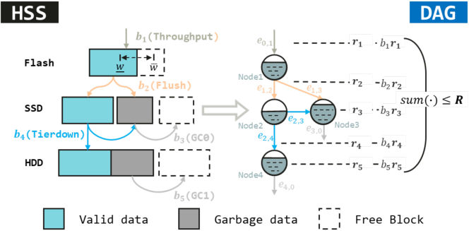
Figure 1. A three-tier hierarchical storage system (left part). The data migration and bandwidth control between tiers can be mapped into a Directed Acyclic Graph (DAG).

2.3. Motivations

The bandwidth control policy proposed for caching and networking optimization cannot be directly applied in HSS without non-trivial modification. To prove it, we design a rule-based bandwidth control policy modified from LBICA (2018LBICA, ) and deploy it at each tier of a commercial HSS. The experimental results suggest that it cannot perform as good as in non-hierarchical storage system, which is recorded as Baseline 1 in Table 1 and Figure 3. It can be inferred that the poor performance of LBICA-like control method in HSS is due to that it cannot cooperatively control multiple bandwidths.

Certainly, the existing bandwidth control policies could still perform good in HSS via elaborate modification but the process must need human experts to make lots of efforts and be time-consuming. Besides, it is expected that the architecture of HSS becomes more complex with the rapid development of storage medium. Then the expert-driven design is undesirable in the future. Thus we would like to design a cooperative bandwidth control policy for HSS which could easily adapt to new architecture with the help of machine learning techniques.

3. Design of PASCAL

3.1. Formulation

In this paper, we use a Directed Acyclic Graph (DAG) $G=(V,E)$ to model the data migration process in HSS, where each node $i\in V$ represents one of the storage tiers (or a class of data stored within a tier such as valid/garbage data in SSD tier) and each directed edge $e_{i,j}\in E$ $(i,j\in V)$ that connects with one pair of nodes $(i,j)$ denotes the data migration relation between the two nodes (see Figure 1). The structure of the DAG can be represented by a matrix $\mathbf{E}=(\mathbf{e}_{ij})_{i,j\in V}$, where the value of $e_{i,j}$ is defined as:

(1) $$e_{ij}=\left\{\begin{array}[]{lr}-1,\text{if }i\to j\\ 1,\text{if }j\to i\\ 0,\text{if }i\nleftrightarrow j\end{array}\right.$$

In the equation above, $\to$ denotes the direction of data migration; $\nleftrightarrow$ represents that there is no connecting relation between the two nodes. For each node $i$, it is described by some indicators including real-time watermark level $w_{i}$ (capacity utilization), maximum capacity $C_{i}\in\mathbb{R}^{+}$, and the lower and upper bound of watermark level ($\underline{w}_{i},\overline{w}_{i}\in[0,1]$ and $\underline{w}_{i}\leq\overline{w}_{i}$). For each edge $e_{i,j}$, its direction denotes the direction of the corresponding data migration and its width $x_{i,j}\in\mathbb{R}$ represent the amount of data migrated from node $i$ to node $j$. For the h$th$ data migration task $\mathbb{B}_{h}$, it comprises one or several edges, which is represented as $e_{i,j}\in\mathbb{B}_{h}$ (see Figure 1). The data migrated by the task is denoted as $d_{h}$ meanwhile the bandwidth assigned to it is denoted as $b_{h}$, which is considered as a consumption of resource. Besides, the bandwidth control will consume a certain amount of other kinds of system resource such as CPU, memory, etc. It is appropriate to assume that there are totally $K$ kinds of resource within the system, each of whom is associated with a upper limit $R_{k}\in\mathbb{R}^{+}$ ($k\in\{1,2,...,K\}$) predefined by the hardware. And $r_{h}^{k}\in\mathbb{R}^{+}$ denotes the amount of resource $k$ consumed by one unit of $d_{h}$. The bandwidth control is a continuous-time process. However, we do not adjust the bandwidth in a high frequency in practice. Instead, for a given time duration $T$ (such as an integral workload or infinite time horizon), it is split into time intervals of equal length $T_{0}$. Thus some above variables will be attached with the timestamp $t$, such as $w_{i}^{t},x_{i,j}^{t},b_{h}^{t}$. Noting that in a real system, the resource consumption per unit bandwidth $r_{h}^{k}$ is indeed time-varying. It can be considered as a random variable subject to time interval $t$ and other system random factors $\xi$. Our goal is to maximize the throughput and meanwhile maintain it stable. Based on above, a mathematical model is given below:

Objective

(2) $$\max\quad\sum_{t=0}^{\lceil T/T_{0}\rceil}x_{0,1}^{t}$$

(3) $$\min\quad\sum_{t=1}^{\lceil T/T_{0}\rceil}(x_{0,1}^{t}-x_{0,1}^{t-1})^{2}$$

s.t.

Watermark Constraints

(4) $$w_{i}^{t}=(w_{i}^{t-1}\times C_{i}+\sum_{i\neq j}x_{j,i}^{t-1}-\sum_{i\neq j}x_{i,j}^{t-1})/C_{i}\quad\forall i,j,t$$

(5) $$\underline{w}_{i}\leq w_{i}^{t}\leq\overline{w}_{i}\quad\forall i,t$$

Data Migration Constraints

(6) $$x_{i,j}=m_{i,j,h}d_{h}\quad e_{i,j}\in\mathbb{B}_{h}$$

Resource Constraints

(7) $$r_{h}^{k}\sim\mathcal{P}(t|\xi)\quad\forall h,k,t$$

(8) $$\sum_{h}d_{h}^{t}r_{h}^{k}\leq R_{k}\quad\forall h,k,t$$

We consider two objectives simultaneously in our problems, namely Eq.(2) and Eq.(3). In above objectives, $x_{0,1}^{t}$ denotes the amount of top-level data migration, which is the throughput of the whole system perceived by client severs. As for the constraints, six categories are included. Eq.(4) defines the watermark level according to the data migration relation; Eq.(5) constrains the watermark level of each node to be within a given range; Eq.(6) represents that the amount of data migrated by an edge is proportional to the amount of data migrated by the corresponding task. Besides, resource consumption is a random process denoted by Eq.(7). The total resource consumption by kinds of data migration task is supposed to be less than resource upper limits, denoted by Eq.(8).

3.2. Core idea

Based on above formulation, we propose our bandwidth control policy, named PASCAL, which is inspired by the concept of equilibrium in physics. Generally, an equilibrium state is stable if it always automatically restores to the original state, even though it deviates from the balance position by disturbance. Furthermore, if there is only one attainable equilibrium among all possible states, the system will always be in a trend of approaching to that equilibrium state. This character is helpful to maintain the watermark levels within proper range, therefore, PASCAL is designed to control the HSS by imitating the action of a system with stable equilibrium. The stable equilibrium in HSS is defined as a state when the system’s watermarks keep at a certain level and bandwidths stay fixed. Assuming that the array of data migration size is denoted as $\mathbf{x}$, the equilibrium state can be represented via:

(9) $$\mathbf{\Delta w}\cdot\mathbf{c} =\mathbf{x}\times\mathbf{E}$$

(10) $$=\mathbf{d}\times\mathbf{M}\times\mathbf{E}$$

(11) $$=\mathbf{0}$$

where $\mathbf{M}$ refers to the mapping matrix of data migration tasks to edges (see Eq.  (6)). For the purpose claimed above, an abstract indicator, namely pressure, is created for each node to guide the data migration relevant with the node. Essentially, pressure is a value mapped from the current state of the node. For any task in the system, its bandwidth depends on the pressure of all the nodes directly effected by it. Generally, the increase of one node’s pressure leads to an increase of the data migrated out the node and a decrease of the data migrated in the node. By this means, the pressure of every node stays constant when the whole system is in equilibrium. On the contrast, if there is any deviation from the equilibrium, the value of pressure goes to change and causes the system return to the equilibrium. Moreover, machine learning method is applied to PASCAL to make it work in a cooperative manner. In the HSS, different nodes have typical functions. As a consequence, the rule to calculate value of pressure is required to be customized, which can be well conducted by machine learning method.

4. Implementation

4.1. Overview

PASCAL mainly consists of two components, namely pressure balancer and bandwidth allocator, as shown in Figure 2. In the pressure balancer, for each node in DAG, we maintain a pressure value according to its real-time watermark level. Then based on the connecting relation between nodes and respective pressure values, the ratio of data to be migrated along edges is derived. As for the bandwidth allocator, it is responsible for calculating the bandwidth controlling results according to data migration ratio derived from the pressure balancer. Since the resource efficiency in HSS is time-varying, the bandwidth allocator is also supposed to consider the real-time resource consumption by one unit of bandwidth. In the following, each module is described at length.

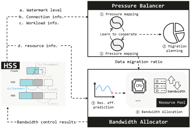
Figure 2. Overview of PASCAL bandwidth control policy. It consists of pressure balancer and bandwidth allocator.

4.2. Pressure balancer

Pressure mapping. For each node $i$ in DAG (i.e., storing tier or part of storing tier within HSS), its pressure value $p_{i}$ denotes how hard data migrates into the node. For example, the larger the pressure is, the harder data moves into the node and vice versa. Generally, the pressure $p_{i}$ is mapped from watermark level $w_{i}$ via a mapping function $\mathcal{F}:w_{i}\mapsto p_{i}$. The expression of mapping function is not restricted here. But it should be with the following properties.

Property 1 (Origin property).

Given an ideal pressure value $p_{i}^{*}$ corresponding to the ideal watermark level $w_{i}^{*}$, the mapping function is supposed to passes through the point of $(w_{i}^{*},p_{i}^{*})$, as shown below:

(12) $$\mathcal{F}(w_{i}^{*})=p_{i}^{*}$$

Property 2 (Non-decreasing property).

The pressure value is supposed to (at least) increase when the watermark level rises, as shown below:

(13) $$\mathcal{F}(w_{i})\geq\mathcal{F}(w_{i}^{{}^{\prime}})\quad\forall w_{i}>w_{i}^{{}^{\prime}}$$

Property 3 (Infinity property).

The pressure value approaches infinity when the watermark level approaches one, i.e.,

(14) $$\lim\limits_{w_{i}\to 1}\mathcal{F}(w_{i})\to\infty$$

Property 1 suggests that the system is able to arrive at the equilibrium, where the ideal watermark level $w_{i}^{*}$ could be determined by human experts or tuned by machine learning techniques and the ideal pressure $p_{i}^{*}$ is obtained by Eq.(11) and Eq.(15). Property 2 ensures that there is only one equilibrium, so that the system must tend to the predefined equilibrium. And Property 3 constrains the occupied capacity of a node to be less than its maximum capacity, which guarantees the system security to some extent.

Data migration planning. Though pressure is capable of guiding the bandwidth related to the corresponding node, a precise method to get the specific value for each bandwidth control task is demanded. Considering that a task is normally associated with several nodes, the rule is made that bandwidth of a task is proportional to its pressure difference. Specifically, the pressure difference of a single edge is calculated by subtract the pressure value of both nodes connected by it. And for a task consisting of several edges, its pressure difference is the weighted average of its edges’ pressure difference. Generally, the ratio of data to be migrated by each task can be calculated via:

(15) $$\mathbf{D}_{norm}=\frac{\mathbf{p}\times(\mathbf{M}\times\mathbf{E})^{T}}{|\mathbf{p}\times(\mathbf{M}\times\mathbf{E})^{T}|_{1}}$$

Learning to cooperation. Above process can calculate the data migration ratio among nodes according to real-time watermark level of each node. However it might not be the best data migration ratio. Because there is no cooperation between different data migration tasks. For example, when the watermarks level of Flash tier is increasing, the most appropriate response is to remain bandwidth of throughput and increase bandwidth of flush, meanwhile decrease the bandwidths of other tasks. This is because throughput is the most significant task in terms of the performance. Therefore, the change of its bandwidth should be treated prudently.

On the other hand, the above process is fully parameterized. Hence it can achieve cooperation between different bandwidth control tasks via machine learning techniques. More specifically, the ideal watermark level $w^{*}_{i}$, which is a hyperparameter, has huge impact on the performance of PASCAL. It is hard for human expert to determine the best $w_{i}^{*}$. And there are many such hyperparameters in HSS (i.e., one node is associated with one ideal watermark level). Considering above, we resort to Bayesian Optimization (0BOA, ) to achieve the learning to cooperation. The experimental results illustrate that the performance of PASCAL can be enhanced greatly using Bayesian optimization (see Section 5.3).

4.3. Bandwidth allocator

Resource efficiency prediction. The run-time environment of the HSS is extremely complex. Various background tasks existing in the system, including bandwidth control, compression, scheduling, deduplication, etc. These tasks might affect each other. For example, these tasks compete for kinds of data access, system resources throughout the run time. It is intractable to fully analyze the mutual influences among them. However it is impractical to assume that the resource efficiency (i.e., $r_{h}^{k}$ the resource consumption by one unit of bandwidth) is constant throughout the control process. Instead, we resort to model the resource efficiency and to predict it when allocating the bandwidth. Specifically, for each $r_{h}^{k}$ (defined in Section 2.2) at time interval $t$, it can be predicted via:

(16) $$\tilde{r}_{h}^{k}=G(\{r_{h}^{k,t^{\prime}}|t^{\prime}=t-1,t-2,...,t-m\})$$

where $\{r_{h}^{k,t^{\prime}}|t^{\prime}=t-1,t-2,...,t-m\}$ is a time series of ground truth value of historical $r_{h}^{k}$; $G$ is the predicting function which can either be classical time series forecasting methods such as ARIMA (2021Visibility, ) or be supervised learning models such as LSTM (2014Long, ; 2016Learning, ). In this way, a predicted resource efficiency matrix $\mathbf{r}$ can be constructed:

(17) $$\mathbf{r}=(\tilde{r}_{h}^{k}),\quad h=1,...,H,k=1,...,K$$

With the data migration ratio and the predicted resource efficiency available, the resource consumption vector $\mathbf{r_{S}}\in\mathbb{R}^{K}$ of the whole system when migrating one unit of data can be obtained:

(18) $$\mathbf{r_{S}}=\mathbf{r}\times\mathbf{D}_{norm}$$

Bandwidth allocation. Taking as input the data migration ratio and resource efficiency prediction, the bandwidth allocation is finished in this module. Specifically, for each bandwidth $b_{h}$, it can be obtained from solving the following equations:

(19) $$\mathbf{b}=(\min\{\frac{R_{k}}{r^{k}}|k=1,2,...,K\})\times\mathbf{D}_{norm}$$

where $\mathbf{b}=(b_{h})\in\mathbb{R}^{H}$ is the bandwidth allocation results derived from PASCAL. After obtaining the results, each related task (such as throughput, flush, garbage collection, etc.) will be noticed with the results and execute incident bandwidth control. Besides, the ground truth value of resource efficiency will be stored for next time prediction.

Algorithm 1 Running process of PASCAL

1:  Input: Architecture of hierarchical storage system (i.e., the DAG), hardware configuration (i.e., upper limit of kinds of resource), pressure mapping function $\mathcal{F}$, resource prediction function $G$

2:  Initialization: 1) For each $r_{h}^{k}$, initialize queue $Q_{h}^{k}=\{\}$ for storing ground truth value of resource efficiency; 2) set timestamp $t=0$

3:  while True do

4:     Pressure mapping: For each node $i$ with water level $w_{i}$, get its pressure value $p_{i}=\mathcal{F}(w_{i})$

5:     Data migration planning: Given real-time workload information, connecting matrix and pressure value of each node, get the data migration ratio among edges $\mathbf{D}_{norm}$ according to Eq.(15).

6:     Resource efficiency prediction: Given queues of historical resource efficiency, predict current resource efficiency $\mathbf{r}$ according to Eq.(16).

7:     Bandwidth allocation: Given $\mathbf{D}_{norm}$ and $\mathbf{r}$, calculate the bandwidth allocation using Eq.(19).

8:     Data recording: record the ground truth value of current resource efficiency and store it into queues.

9:     $t=t+1$

10:  end while

4.4. Summary & Discussion

To summarize the whole procedure of PASCAL, a snippet of pseudo code is given in Algorithm 1. The procedure and function of each module within PASCAL are described above. However, we do not claim that our recommended implementation of PASCAL is the best one but it outperforms other heuristic method, which is shown in experiments. Readers of interest could adopt other techniques to implement modules of PASCAL, to further enhance its performance. For example, the pressure mapping function could be either designed by human expert or learned by neural network (2022Artificial, ), Bayesian optimization method (0BOA, ); The resource efficiency prediction could be improved using transformer (DBLP:journals/corr/VaswaniSPUJGKP17, ). The further discussion is beyond the scope of the paper. A valid explanation for the effectiveness of PASCAL is that it has a structure similar to a neural network, where the pressure mapping functions as an active layer and data migration planning resembles a connected layer. Due to this structure, PASCAL is able to deal with various situation appropriately.

5. Evaluation

5.1. Methodologies

Testbed. To verify the effectiveness of PASCAL, all experiments are conducted in a commercial HSS, Huawei OceanStor Dorado 5210 V5. The storage system is with 24-core 2.6GHZ CPU*2, 64GB RAM*8 (as caching tier), 0.96TB SSD*8 (as SSD tier) and 0.96T SAS*48 (as HDD tier).

Workloads. Two categories of workload, i.e., the synthetic workloads and real-world workloads are used in the experiments. The synthetic workloads are generated using the open-source benchmarking toolkit Vdbench (2010VDBench, ) which is commonly used to evaluate the storage system. We can easily generate 20 workloads via tuning the parameters of the tool (such read/write mix, queue depth, block size, IO size, etc). While five real-world workloads are collected from our customers, which is anonymized due to the business security requirements. For conciseness of experiments, within each category we merge different workloads and process them into one workload which lasts 25,000 seconds.

Comparing targets. Three rule-based methods are used as baseline to evaluate PASCAL, of which each is described concisely below:

• Baseline 1 is a rule-based control method modified from LBICA (2019LBICA, ), which is implemented at each tier. In simple terms, for one storing tier, Baseline 1 will greatly reduce the bandwidth of data migration into the tier once it finds that the capacity utilization of the tier is beyond a given threshold.

• Baseline 2 is a derivative of the classic PID controller (2005PID, ), where bandwidth is the controlling object and we replace the integral of the bandwidth with corresponding watermark level.

• Baseline 3 is a systematic bandwidth control scheme adopted in Huawei’s current storage products. The detailed techniques can be referred to (oceanstor, ).

Metrics of interest. The 99%th tail latency, mean throughput and throughput jitter are mainly considered in our evaluation. Note that the throughput jitter is measured using

(20) $$\sqrt{\frac{\sum_{t=0}^{T}(I_{t}-\overline{I_{t}})^{2}}{T}}/\overline{I_{t}}\quad\quad\quad$$

where $I_{t}$ is the throughput at time interval $t$ and $\overline{I_{t}}$ is the average throughput during the workloads. We expect the storage system to have low IO latency, low throughput jitter and high mean throughput simultaneously.

5.2. Performance evaluation

The performance comparison among PASCAL and baselines were carried out over the two workloads. The results are reported in Table 1. To be more intuitive, the above results are visualized in Figure 3. As is shown in Figure 3, PASCAL outperforms all compared baselines in terms of throughput jitter (at least 2X improvement) and tail latency (at least 1.95X improvement), which achieves parts of our optimization goals. Meanwhile, PASCAL is able to maintain high mean throughput. Specifically, on the synthetic workload PASCAL can achieve the highest mean throughput (1282.98 MB/s) among all compared methods; For the real-world workload, the mean throughput performance with PASCAL is a little bit lower than that of other methods but still comparable. That PASCAL achieves such a good performance on tail latency and throughput jitter is due to the global view of data migration planning. Besides, PASCAL prefers to sacrifice throughput to gain the improvement of performance stability, which is in accordance with the purpose of clients.

Table 1. Summary of performance evaluation results

Workload	Method	Mean throu. (MB/s)	Tail latency (ms)	Throu. jitter
Synthetic	Ours	1282.98	22.36	3.37e-02
	Baseline 1	1269.97	150.97	7.95e-02
	Baseline 2	1273.08	244.69	1.49e-01
	Baseline 3	1253.17	170.62	7.53e-02
Real-world	Ours	1277.56	52.31	3.87e-02
	Baseline 1	1310.23	129.85	9.02e-02
	Baseline 2	1303.14	252.40	1.50e-01
	Baseline 3	1283.61	155.92	7.61e-02

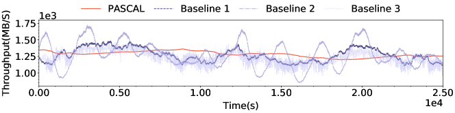
(a) Compared results over synthetic workload

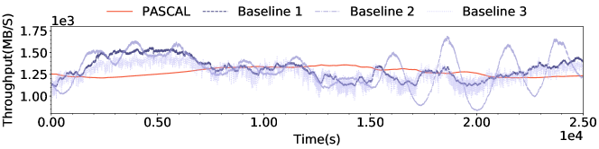
(b) Compared results over real-world workload

Figure 3. Visualization of overall performance evaluation

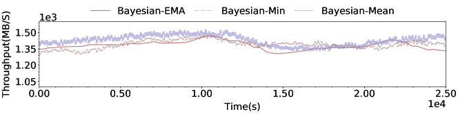
(a) Bayesian optimization inside PASCAL on synthetic workload

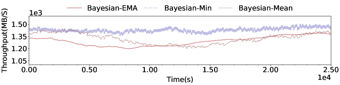
(b) Bayesian optimization inside PASCAL on real-world workload

(c) Without Bayesian optimization inside PASCAL on synthetic workload

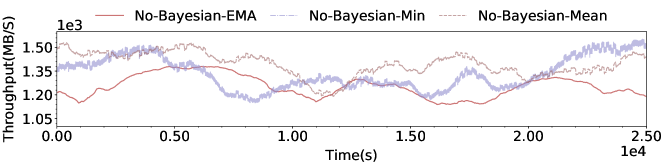
(d) Without Bayesian optimization inside PASCAL on real-world workload

Figure 4. Evaluation result of ablation studies

5.3. Ablation studies

According to the discussion in Section 4.4, many alternative algorithms can be incorporated into PASCAL to further improve its performance. Here we first investigate how PASCAL behaves with and without Bayesian optimization to testify the significance of cooperation. The form of mapping function is fixed as follows:

(21) $$p=p^{*}(\frac{1-w^{*}}{1-w})^{\alpha}$$

where $\alpha$ and $w^{*}$ are the hyperparameters need to be tuned. Besides, we investigate how PASCAL behaves with various implementations of resource efficiency prediction. Three simple methods as the predicting function are adopted, namely Exponential Moving Average (EMA) (DBLP:journals/eswa/NakanoTT17, ), mean and min function of historical data. To this end, a queue with length of 50 is maintained to store the historical resource efficiency data. With above setting, the ablation studies were performed over the two workloads. The results are reported in Figure 4. Observed from the results, it is obvious that PASCAL with Bayesian optimization performs much better than one without finely tuned mapper function in terms of throughput jitter. Besides we also find that PASCAL is not much sensitive to the accuracy of resource efficiency prediction because there is no great difference in terms of throughput jitter when using various resource prediction function. However, more advanced prediction tools and models such as transformer (DBLP:journals/corr/VaswaniSPUJGKP17, ) might bring more performance improvement into PASCAL, which is left to the future work.

6. Conclusion

In this paper we investigate the bandwidth control problem in the hierarchical storage system. We design and implement a learning-aided cooperative control policy PASCAL, which regards the problem as a pressure balancing problem. Our evaluation shows that PASCAL can effectively decrease the throughput jitter and tail latency of the system, and meanwhile keep the throughput at a relatively high level. PASCAL is expected to be fully deployed in our commercial hierarchical storage product.

References

- [1] David Vengerov. A reinforcement learning framework for online data migration in hierarchical storage systems. J. Supercomput., 43(1):1–19, 2008.
- [2] T. G. Lakshmi and R. R. Sedamkar. Proactive and adaptive data migration in hierarchical storage systems using reinforcement learning agent. International Journal of Computer Applications, 94(9):46–52, 2014.
- [3] A. Verma et al. An architecture for lifecycle management in very large file systems. In 22nd IEEE / 13th NASA Goddard Conference on Mass Storage Systems and Technologies (MSST 2005), Information Retrieval from Very Large Storage Systems, CD-ROM, 11-14 April 2005, Monterey, CA, USA, 2005.
- [4] M. Kunjir et al. Robus: Fair cache allocation for multi-tenant data-parallel workloads. Computer Science, 2015.
- [5] Jaehyung et al. Selective i/o bypass and load balancing method for write-through ssd caching in big data analytics. IEEE Transactions on Computers, 67(4):589–595, 2017.
- [6] Saba Ahmadian et al. Lbica: A load balancer for i/o cache architectures. In 2019 Design, Automation & Test in Europe Conference & Exhibition (DATE), 2019.
- [7] S. Ahmadian, R. Salkhordeh, and H. Asadi. Lbica: A load balancer for i/o cache architectures. 2018.
- [8] M. Pelikan et al. Boa: The bayesian optimization algorithm. Morgan Kaufmann Publishers Inc.
- [9] A. G. Salman et al. Visibility forecasting using autoregressive integrated moving average (arima) models. Procedia Computer Science, 179:252–259, 2021.
- [10] H. Sak et al. Long short-term memory recurrent neural network architectures for large scale acoustic modeling. computer science, 2014.
- [11] H. C. Ravichandar et al. Learning and predicting sequential tasks using recurrent neural networks and multiple model filtering. 2016.
- [12] A. Seem et al. Artificial Neural Network, Convolutional Neural Network Visualization, and Image Security. Soft Computing: Theories and Applications, 2022.
- [13] Ashish Vaswani et al. Attention is all you need. CoRR, abs/1706.03762, 2017.
- [14] A. Berryman et al. Vdbench: A benchmarking toolkit for thin-client based virtual desktop environments. In IEEE Second International Conference on Cloud Computing Technology & Science, 2010.
- [15] K. H. Ang et al. Pid control system analysis, design, and technology. IEEE Transactions on Control Systems Technology, 13(4):p.559–576, 2005.
- [16] Huawei. Understanding the cache performance of huawei oceanstor storage system v300r003, 2021.
- [17] Masafumi Nakano et al. Generalized exponential moving average (EMA) model with particle filtering and anomaly detection. Expert Syst. Appl., 73:187–200, 2017.