Very metal-poor stars in the solar vicinity: kinematics and abundance analysis

Abstract

Very metal-poor stars contain crucial information on the Milky Way’s infancy. In our previous study (Plotnikova et al., 2022) we derived a mean age of $\sim$ 13.7 Gyr for a sample of these stars in the Sun’s vicinity. In this work, we investigate the chemical and kinematics properties of these stars with the goal of obtaining some insights on their origin and their parent population. We did not find any Al-Mg anti-correlation, which lead us to the conclusion that these stars did not form in globular clusters, while the detailed analysis of their orbital parameters reveals that these stars are most probably associated with the pristine Bulge of the Milky Way. We then sketch a scenario for the formation of the Milky Way in which the first structure to form was the Bulge through rapid collapse. The other components have grown later on, with a significant contribution of accreted structures.

1 Introduction

Very metal-poor stars are one of the best candidates to study the formation and evolution of the Universe and its Galactic components. The study of their chemistry and kinematics can help us to understand the chemical and dynamical properties of the first Population III supernovae. The origin of these stars contains important information about the Milky Way formation history.

Theoretical simulations of the Galaxy formation (Bullock & Johnston (2005)) have shown that the Halo bears the signatures of the Milky Way’s assembly from smaller “building block” galaxies. Recent astrometric studies have shown the existence of kinematic signatures that indicate past accretion events (Belokurov et al. (2018); Myeong et al. (2019); Yuan et al. (2020)). That means that the kinematics of very metal-poor stars is an important testbed of the Galaxy formation and evolution theories. In fact, stars with very low metal abundances are potential members of accreted dwarf galaxies and/or clusters.

Two main theories were suggested for the Milky Way formation. The first theory is the hierarchical scenario which tells us that our Galaxy was formed through the hierarchical merging of smaller dark halos. The accretion of baryonic matter occured later. The Bulge was formed first, followed by the Thin Disk. The Thick Disk could have been produced by the kinetic heating induced by small/medium mass engulfing companions.

The presence of stellar streams in the stellar Halo supports the hierarchical scenario (Helmi (2002), Ibata et al. (2002)): they are tidal remains of past merging events (Grillmair (2017)). Nowadays, we have a number of confirmed accreted events such as Sagittarius dwarf galaxy, Gaia-Enceladus-Sausage, Sequoia, Helmi stream, Thamnos, while other streams were found to be associated with accreted globular clusters (Koppelman et al. (2019)). The Halo of the Galaxy could have mostly be assembled in a sequence of minor mergers. Furthermore, the fact that the merging frequency is increasing with redshift, tells us that in the infant Galaxy merging events were quite common. That lends further support to the hierarchical scenario.

The second and most successful scenario is Secular Evolution (SE), with slow but continuous external matter accretion. According to this theory, the Bulge of the Galaxy was formed due to the accretion of disk matter through bar instabilities. This scenario is in agreement with the observed color gradient and the relation between the color of the bulge and disk studied through statistical analysis of 257 spiral galaxies (Gadotti & dos Anjos (2001)). SE is also supported by the relation between the bulge and disk masses and radii (Courteau et al. (1996)).

Metal-poor stars, being mostly ancient, are ideal probes of the early evolutionary phases of the Universe. Because of their low metallicity, they are linked to the most pristine star formation episodes in the Universe.

In this work, we build on (Plotnikova et al., 2022) and study the kinematics and abundances of a sample of very metal-poor stars in the solar vicinity. Therefore, the layout of this study is as follows. In Section 2 we discuss the data upon which our study is based. Section 3 and 4 are focused on the chemistry and kinematics of our stars, respectively. The results of our investigation are detailed in Section 5, while Section 6, finally, summarizes the outcome of this study and highlights future perspectives.

2 Data

As the main target for this investigation, we chose the data set of 28 very metal-poor stars for which we derived precise ages (Plotnikova et al. (2022)). These stars are of particular interest because they are very metal-poor and their average age is $13.7\pm 0.4$ Gyr. As a result, the stars in this sample are valuable candidates to study the early stages of the Galaxy formation.

2.1 Distance determination

Distance is one of the most important parameters in dynamics studies. In Plotnikova et al. (2022) we compared the best distances, estimated out of four different techniques: Gaia DR3 parallaxes (Gaia Collaboration et al. (2022)), Gaia EDR3 (Gaia Collaboration (2021)) corrected by Lindegren et al. (2021), the distances derived by Bailer-Jones et al. (2021), and Queiroz et al. (2019) (StarHorse). Our choice was made based on the best fit of the data with the isochrones in the color-magnitude diagram. As a result, we found that the best distances are those obtained directly from Gaia DR3 parallaxes (Plotnikova et al. (2022)).

2.2 Astrometric parameters

With the goal of calculating orbits and orbital parameters, we extracted coordinates, radial velocities, and proper motion components from the Gaia DR3 archive (Gaia Collaboration et al. (2022)). Uncertainties for velocity components are shown in Tab.1, 2. Position and velocity of the stars in the Equatorial Coordinates were transformed to Galactocentric coordinates by astropy python package.

Data product or source type	Typical uncertainty, km s-1
	G${}_{RVS}<$ 8	GRVS = 10	GRVS = 11.75
Median radial velocity over 22 months	0.3	0.6	1.8
Systematic radial velocity errors	$<$ 0.1	-	0.5

Table 1: Uncertainties of Gaia Early Data Release 3 proper motions

Data product or source type	Typical uncertainty
	G $<$ 15	G = 17	G = 20	G = 21
Five-parameter astrometry
position, mas	0.01 - 0.02	0.05	0.4	1
parallax, mas	0.02 - 0.03	0.07	0.5	1.3
proper motion, mas yr-1	0.02 - 0.03	0.07	0.5	1.4
Six-parameter astrometry
position, mas	0.02 - 0.03	0.08	0.4	1
parallax, mas	0.02 - 0.04	0.1	0.5	1.4
proper motion, mas yr-1	0.02 - 0.04	0.1	0.6	1.5

Table 2: Uncertainties of Gaia Early Data Release 3 astrometry Gaia Collaboration (2021)

3 Chemistry

All our stars are from Hamburg vs. ESO R-process Enhanced Star (HERES) survey. The chemical abundances were spectroscopically studied by Barklem et al. (2005). The spectrum synthesis assumes LTE and a 1D plane-parallel model of the atmosphere, where turbulence is modeled through the classical micro-turbulence and macro-turbulence parameters. Their snapshot spectra cover a wavelength range of 3760 – 4980 Å and have an average signal-to-noise ratio of S/N $\sim$ 54 per pixel over the entire spectral range. A $2^{\prime\prime}$ slit is employed giving a minimum resolving power of $R\approx$ 20000. From the ”snapshot” spectra the elemental abundances of moderate precision (absolute r.m.s. errors of order 0.25 dex, relative r.m.s. errors of order 0.15 dex) have been obtained for 22 elements: C, Mg, Al, Ca, Sc, Ti, V, Cr, Mn, Fe, Co, Ni, Zn, Sr, Y, Zr, Ba, La, Ce, Nd, Sm, and Eu. The abundances used in this work are listed in Tab.3.

ID	[Mg/Fe]	[Al/Fe]LTE	[Al/Fe]NLTE	[Ca/Fe]	[Cr/Fe]	[Ti/Fe]	[Ni/Fe]	[Fe/H]	age	Origin*
	dex	dex	dex	dex	dex	dex	dex	dex	Gyr
HE_0023-4825	0.22	-1.01	-0.51	0.26	0.00	0.31	-0.01	-2.06	14.62 $\pm$ 0.11	Pr.B.
HE_0109-3711	-	-	-	0.42	-0.06	0.38	-	-1.91	11.78 $\pm$ 0.04	5G/GE
HE_0231-4016	0.22	-1.09	-0.50	0.36	-0.11	0.25	-0.14	-2.08	14.37 $\pm$ 0.47	Pr.B.
HE_0340-3430	0.19	-1.00	-0.61	0.36	-0.16	0.25	-0.26	-1.95	13.32 $\pm$ 0.13	5G/GE
HE_0430-4404	0.29	-0.97	-0.57	0.33	-0.02	0.32	0.01	-2.07	10.15 $\pm$ 1.38	Th.1
HE_0447-4858	0.24	-0.81	-0.42	0.24	0.09	0.28	0.33	-1.69	13.28 $\pm$ 0.20	5G/GE
HE_0501-5139	0.19	-	-	0.34	-0.24	0.39	-0.13	-2.38	8.93 $\pm$ 0.03	Th.1
HE_0519-5525	0.41	-0.76	-0.26	0.37	-0.19	0.37	0.13	-2.52	13.46 $\pm$ 0.06	5G/GE
HE_0534-4615	0.22	-0.87	-0.37	0.28	-0.18	0.19	-0.20	-2.01	14.91 $\pm$ 0.49	Pr.B.
HE_1052-2548	0.16	-0.48	-0.11	0.27	-0.12	0.45	0.03	-2.29	15.70 $\pm$ 0.14	Pr.B.
HE_1105+0027	0.47	-0.89	-0.33	0.47	0.05	0.32	-0.29	-2.42	12.06 $\pm$ 0.35	Th.1
HE_1225-0515	0.18	-1.00	-0.62	0.27	-0.08	0.34	-0.16	-1.96	14.64 $\pm$ 0.03	Pr.B.
HE_1330-0354	0.32	-0.93	-0.46	0.40	-0.05	0.54	-0.08	-2.29	13.49 $\pm$ 0.34	SimD
HE_2250-2132	0.31	-1.07	-0.57	0.29	-0.12	0.35	0.05	-2.22	13.19 $\pm$ 0.11	SimD
HE_2347-1254	0.29	-0.74	-0.42	0.37	-0.13	0.39	-0.16	-1.83	14.56 $\pm$ 0.03	Pr.B.
HE_2347-1448	0.13	-1.11	-0.64	0.21	-0.05	0.31	0.27	-2.31	8.63 $\pm$ 0.07	5G/GE
HE_0244-4111	0.34	-	-	0.37	-0.19	0.30	0.00	-2.56	12.75 $\pm$ 0.51	Th.1
HE_0441-4343	0.32	-1.09	-0.59	0.18	-0.36	0.27	0.07	-2.52	10.41 $\pm$ 0.50	Th.1
HE_0513-4557	0.34	-	-	0.21	-	-	-	-2.79	12.42 $\pm$ 0.50	OrNC
HE_0926-0508	0.28	-0.90	-0.49	0.37	-0.14	0.49	-0.06	-2.78	14.79 $\pm$ 0.51	Pr.B.
HE_1006-2218	-	-0.79	-0.46	0.32	-0.11	0.48	-	-2.69	12.90 $\pm$ 0.51	Th.2
HE_1015-0027	0.35	-1.00	-0.67	0.41	-0.24	0.55	-0.10	-2.66	15.20 $\pm$ 0.55	Pr.B.
HE_1126-1735	0.31	-1.06	-0.46	0.32	-0.29	0.33	-0.04	-2.69	9.44 $\pm$ 0.50	GE
HE_1413-1954	-	-	-	0.33	-	-	-	-3.22	14.20 $\pm$ 0.82	Pr.B.
HE_2222-4156	0.42	-0.93	-0.42	0.35	-0.21	0.33	-0.02	-2.73	13.50 $\pm$ 0.52	Th.1
HE_2325-0755	0.31	-1.02	-0.42	0.46	-0.29	0.35	-0.18	-2.85	13.50 $\pm$ 0.51	SimD

*GE - Gaia-Enceladus/Sausage, Th.1 - Thamnos 1, Th.2 - Thamnos 2, Pr.B. - primordial bulge, 5G/GE - 5 stars group, high probability to belong to the GE, SimD - similar to the disk kinematics, OrNC - origin is not clear, stars have halo kinematics and chemistry.

Table 3: Chemistry

3.1 Non-LTE corrections

As mentioned above, spectral analysis in Barklem et al. (2005) was done assuming only the LTE model. However, aluminum abundance was obtained from the lines in the ultra-violet part of the spectrum that are significantly affected by Non-LTE effects (Nordlander & Lind (2017)). To improve the precision of the chemical parameters we applied Non-LTE correction from Nordlander & Lind (2017). The correction was implemented for each star according to its effective temperature ($T_{eff}$), metallicity ($[Fe/H]$) and gravity ($logg$). The resulting obtained corrections are on average around 0.5 dex (Tab.3).

We also checked Non-LTE corrections for all other elements by means of MPIA webtool database but in all cases, corrections are less than 0.1 dex and were considered negligible.

4 Kinematics

We obtained orbits and orbital parameters for all stars in the data set using parallaxes, proper motion and radial velocities from Gaia DR3 by numerical calculation and adopting a model of Galactic potentials. The results are then analyzed to obtain insights on the stars’ origin.

4.1 Galactic axisymmetric potential

We corrected the velocities of the stars by the velocity of the Sun with respect to the Galactic center which is computed independently from the velocity of the local standard of rest (Reid & Brunthaler (2004), GRAVITY Collaboration et al. (2018), Drimmel & Poggio (2018)):

$$v_{R\odot}=-12.9\pm 3.0\text{kms}^{-1}$$ (1)

$$v_{\phi\odot}=245.6\pm 1.4\text{kms}^{-1}$$ (2)

$$v_{Z\odot}=7.78\pm 0.09\text{kms}^{-1}$$ (3)

where the distance between the Galactic center and the Sun is $R_{0}=8.122\pm 0.033$ kpc (GRAVITY Collaboration et al. (2018)).   We used the McMillan (2017) Galactic potential without bar implementation in galpy (Bovy (2015)) to calculate orbits and orbital parameters such as the total energy ($E_{n}$), eccentricity ($e$), apo-center ($R_{apo}$), and peri-center ($R_{peri}$).

4.2 Galactic non-axisymmetric potential

To take into account the effect of the bar we replaced the axisymmetric bulge from McMillan (2017) with a non-axisymmetric elongated bar/bulge component. As a model for the bar/bulge structure, we used the rotating ellipsoid (Chemel et al. (2018), Yeh et al. (2020)) with density distribution given by Ferrers formula:(Bovy (2015)):

$$\rho(x,y,z)=\left\{\begin{array}[]{lcl}\rho_{c}(1-m^{2})^{2}&,&\text{if}m<1,\\ 0&,&\text{if}m>1,\\ \end{array}\right.$$ (4)

where $m^{2}=\frac{x^{2}}{a^{2}}+\frac{y^{2}}{b^{2}}+\frac{z^{2}}{c^{2}}$. For the parameters, we used $a=5$ kpc, $b=2$ kpc, $c=1$ kpc which gives a good approximation for the observed bar/bulge component in the center of the Milky Way (Portail et al. (2015), Portail et al. (2017)). The central density of the bar is given by $\rho=\frac{105}{32\pi}\frac{GM_{b}}{abc}$, where the mass of the bar $M_{b}=1.88\times 10^{10}$ M_⊙ (Portail et al. (2017)).

The Milky Way bar is rotating around the Galactic center with constant angular velocity $\Omega_{b}$. Also, its major axis is tilted with respect to the Sun.

Recent measurements of bar angular velocity give the following results: $\Omega_{b}=41\pm 3$ km s^-1 kpc^-1 (Sanders et al. (2019)), $\Omega_{b}=37.5$ km s^-1 kpc^-1 (Clarke et al. (2019)), $\Omega_{b}=40$ km s^-1 kpc^-1 (Sormani et al. (2015)). In this work we used bar angular velocity $\Omega_{b}=40$ km s^-1 kpc^-1 which is in a good agreement with Portail et al. (2015), Portail et al. (2017), and Bovy et al. (2019). For the bar orientation relative to the Sun we used $\phi=28^{o}$ which is in good agreement with recent estimates (Wegg & Gerhard (2013), Bland-Hawthorn & Gerhard (2016), and Portail et al. (2017)).

4.3 Uncertainty

To estimate uncertainties for each derived orbital parameter we perform a Monte Carlo analysis using 1000 random draws on the input parameters: parallax, radial velocity and proper motion. We considered errors in right ascension (RA) and declination (DEC) to be negligible compared to other parameters. As for proper motion, we used the multivariate normal distribution which takes into account the correlation between both components. For parallax and radial velocity we used just normal distribution.

Since we use parallaxes, the resulting distribution of each orbital parameter is not Gaussian. Therefore, we derived for each orbital parameter a median value and a confidence interval of 68%.

5 Results

We studied the chemical composition and kinematics of our data set of 28 metal-poor stars and the correlation with their age.

5.1 Chemistry

In Fig.1 we compared the chemical composition of our data set with bulge (red open triangles, Howes et al. (2016)) and halo (grey circles, Yong et al. (2013), Roederer et al. (2014)) stars of the Milky Way. Inspecting this figure one can readily see that all our stars are in good agreement with the typical trends for Milky Way stars. This holds except for aluminum, whose position is shifted on average by 0.2 dex. For all stars we applied non-LTE correction from Nordlander & Lind (2017) that play important role in aluminum abundance.

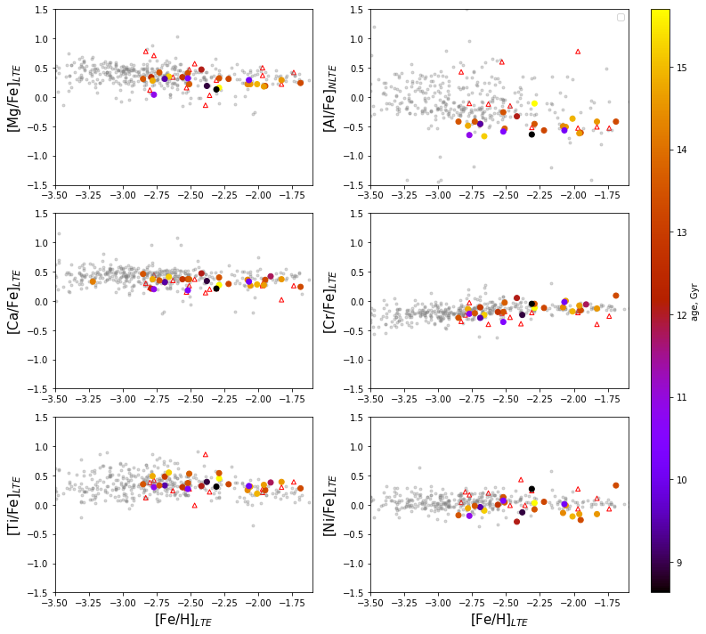
Figure 1: Correlation between iron and other chemical elements color-coded with the age. For comparison we show Bulge (red open triangles, Howes et al. (2016)) and Halo (grey circles, Yong et al. (2013), Roederer et al. (2014)) stars of the Milky Way. For all sources Al correction from Nordlander & Lind (2017) was applied.

To separate stars from the Halo, the Thin, and the Thick disk stars we used the Al versus Mg map (Fig.2). For comparison we used for Disk: Fulbright (2000), Reddy et al. (2003), Simmerer (2004), Reddy et al. (2006), François et al. (2007), Johnson et al. (2012), Johnson et al. (2014); for Halo: Yong et al. (2013), Roederer et al. (2014); and for Bulge: Howes et al. (2016). All our stars having measures for both elements occupy the expected region for halo stars. At odds with globular clusters’ stars, our sample stars do not show any Al-Mg anti-correlation (Lucey et al. (2022), Sestito et al. (2022)).

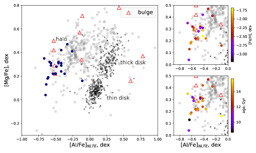
Figure 2: Al-Mg correlation. Top right: color-coded with metallicity, bottom right: color coded with age. The background: disk stars (black dotes, Fulbright (2000), Reddy et al. (2003), Simmerer (2004), Reddy et al. (2006), François et al. (2007), Johnson et al. (2012), Johnson et al. (2014)), halo stars (grey points, Yong et al. (2013)), Roederer et al. (2014), bulge stars (red open triangles, Howes et al. (2016)).

We can therefore conclude that our stars possess the typical chemical composition of the Milky Way Halo field stars. The lack of any anti-correlation seems to exclude an origin inside globular clusters.

5.2 Kinematics

To get additional insight on the origin of these stars we explore their kinematical properties. To this aim, in Fig.3 we compared our results with Koppelman et al. (2019). We used the same McMillan (2017) potential as in Koppelman et al. (2019) but, after checking that there are no differences, we adopted the most recent estimates of the Sun’s velocity and distance to the Galactic center (Sec.4.1). Fig.3 shows that some of the stars share the same kinematics as well-known accretion events: the Gaia-Enceladus/Sausage system (orange; Belokurov et al. (2018), Helmi et al. (2018)) and Thamnos 1,2 (darkblue,blue; Koppelman et al. (2019)). This result is also supported by the velocity and $L_{z}$-eccentricity diagrams (Fig.4).

Besides, we can notice a group of 5 stars below the Gaia-Enceladus/Sausage locus with similar orbital parameters, age, and metallicity, and location inside the sphere with radius R$\sim$1 kpc. In some sources, Gaia-Enceladus/Sausage locus is extended to lower energies (Koppelman et al. (2019)) which gives a higher probability for this 5 stars group to be indeed part of Gaia-Enceladus/Sausage. Moreover, there are three stars (Fig.4, black dotes) that exhibit disk kinematics, although their chemistry looks more similar to the halo .

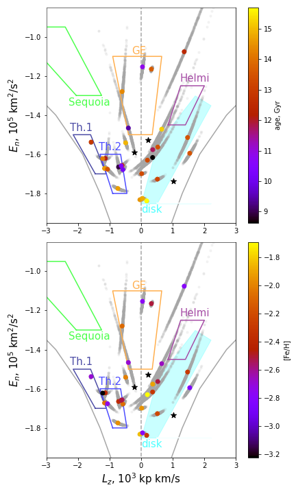
Figure 3: $E_{n}-L_{z}$ diagram with the loci of the biggest known accretion events: Gaia-Enceladus/Sausage (GE) (orange), Helmi stream (purple), Sequoia (green), Thamnos 1, 2 (darkblue, blue); and disk (cyan). Black star symbols indicate Vandenberg halo stars VandenBerg et al. (2014). The colored points are mean values of stars under investigations, while grey trails indicate their uncertainties.

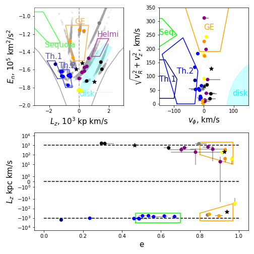
Figure 4: Points are color-coded with the position in $E_{n}-L_{z}$ diagram: Gaia-Enceladus/Sausage (GE) (orange), Sequoia (green), Thamnos 1, 2 (Th.) (dark blue, blue), Sagittarius (red), disk (black), group of 5 stars with similar parameters (purple), low energy stars (yellow), Vandenberg stars VandenBerg et al. (2014) (black stars).

Our stars exhibit both prograde and retrograde motion and they cover almost the entire eccentricity range (Fig.4, lower panel). Additionally, all stars are distributed around $v_{\phi}=0$ km/s which indicates a typical Halo kinematics (Fig.4, upper right panel). They might be part either of Gaia-Enceladus/Sausage (GE) (orange), or of Thamnos 1, 2 (dark blue, blue) accretion events. All diagrams in Fig.4 are color-coded according to their position in the $L_{z}-E_{n}$ diagram (Fig.4, upper left panel)

However, the kinematic analysis alone is not sufficient to identify the origin of these stars and decipher whether they are associated or not with a specific accreted structure. To check the possible membership of blue and orange stars to Gaia-Enceladus/Sausage (GE) (orange) or Thamnos 1, 2 (dark blue, blue) we need to combine kinematics with chemistry. In Fig.5 we can see that both Milky Way stars and accretion events possess similar chemistry.

Overall, our metal-poor stars have chemistry compatible with accretion event trends. Additionally, we compared the age of the stars with the age of each accretion event (Fig.6) and a part of the star’s ages fall into the range of the beginning of the accreting blocks’ formation. But some of the stars from this work are older and can be excluded from being accreted through known accretion events.

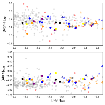
Figure 5: Correlation between Mg, Al and Fe. For comparison, we showed bulge (red circles, Howes et al. (2016)) and halo (grey circles, Yong et al. (2013), Roederer et al. (2014)) stars of the Milky Way. Points are color-coded with the position in $E_{n}-L_{z}$ diagram: Gaia-Enceladus/Sausage (GE) (orange), Sequoia (green), Thamnos 1, 2 (Th.) (dark blue, blue), Sagittarius (red), disk (black), group of 5 stars with similar parameters (purple), low energy stars (yellow). Circles - stars from this work, open triangles - stars from known accretion events Koppelman et al. (2019)).

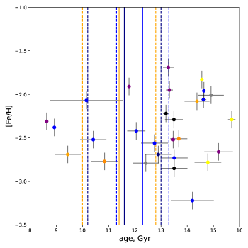
Figure 6: Age-metallicity relation with the time bars of the Gaia-Enceladus/Sausage (GE) (orange), Thamnos 1, 2 (dark blue, blue) formation (Ruiz-Lara et al. (2022)). Solid lines are mean values and dashed lines represent uncertainties.

5.3 Orbital parameters

In Fig.7 we presented the correlation between eccentricity ($e$), peri-centre ($R_{peri}$), maximum height above the galactic plane ($Z_{max}$) and apo-centre ($R_{apo}$) color-coded with age. From the upper plot in Fig.7 we can notice that almost all stars in our data set cross the bulge region. That means that these stars’ kinematics is perturbed by the bar/bulge potential. One can also speculate that they can be a part of the pristine bulge of the Milky Way. From the middle plot in Fig.7 we can see that the most distant stars exhibit on average more elongated orbits. The lower plot in Fig.7 shows that most of the stars have $R_{apo}>Z_{max}$, i.e. they lie close to the Galactic plane. Another intriguing evidence in this plot is that one can readily see a clear trend in age: the oldest stars (yellow) are located lower to the plane while the younger (redder) stars lie closer to the dashed line $R_{apo}=Z_{max}$.

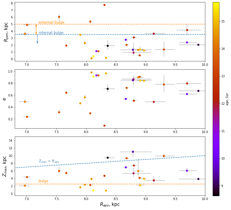
Figure 7: Correlation between eccentricity ($e$), pericentre ($R_{peri}$), maximum height under the galactic plane ($Z_{max}$) and apocentre ($R_{apo}$) color-coded with age.

By inspecting Fig.8 we can highlight also the following trends:

• Eccentricity is increasing with increasing age.

• The older stars orbit closer to the Galactic center and the Galactic disk.

5.3.1 Very old stars

Let us draw our attention to stars with ages larger than $13.5$ Gyr. Their age implies they have a very low probability to be part of any well-known accretion events (Fig.6). Additionally, their age is very close to the age of the Universe and the very first instants of the Milky Way formation. We then speculate that they can have formed inside the very first ”building blocks” of the Milky Way and therefore were part of the infant bulge at a time when the Disk had yet to form (Carraro et al. (1999)).

Moreover, all of them have orbits close to the Galactic Disk and pass close to the Galactic center while crossing the Galactic bulge. This might lend further support to a scenario in which these stars were formed in a pristine Bulge and later displaced in larger eccentricity orbits by some migration phenomenon. The same result was obtained by Grenon (1985) for metal-rich bulge stars in the solar vicinity. However, closeness to the galactic plane is rather the result of the observational limitations (all of our stars lie inside 5 kpc sphere around the Sun) than an intrinsic feature. We consider that with better observations there is a probability to find old metal-poor stars passing through the bulge in elongated orbits in all directions from the Galactic center.

Moving back to chemistry, stars under investigation are $\alpha$-enhanced, and close to typical of today’s Milky Way Halo stars. Speaking about bulge stars, according to Howes et al. (2016) data, chemical composition of Bulge stars is more disperse than Halo stars but distributed around the same mean that makes it impossible to distinguish between Bulge and Halo stars. Still, and interestingly, for all stars in our data set there is a clear correlation between the abundance of $\alpha$-elements and age (Fig.9) with weighted Person correlation coefficient equal to 0.24. This is due to the fact that for low metallicity stars the main source of $\alpha$-elements is supernovae of type II (SNe II). An increasing $\alpha$-abundance can be a signature of an environment where gas density and star formation were quite high. This seems to be another argument in favour of the idea that our oldest stars were associated with the ancient bulge.

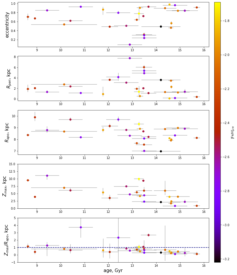
Figure 8: Correlation between eccentricity ($e$), pericentre ($R_{peri}$), apocentre ($R_{apo}$), maximum height under the galactic plane ($Z_{max}$), $Z_{max}/R_{apo}$ and age color-coded with metallicity.

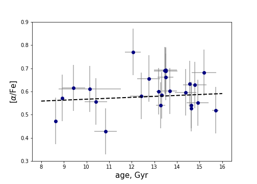
Figure 9: Correlation between $\alpha$-elements and age. The dashed line shows the weighted fit.

5.4 Non-axisymmetric bar/bulge potential

Since most of our stars orbit close to the Galactic center ($R_{peri}<3.5$ kpc) we additionally studied their kinematics in a non-axisymmetric bar/bulge potential (Sec.4.2).

In Fig.10 we can see that first of all changing the potential modifies the total energy ($E_{n}$) that stars possess nowadays. Besides, in their motion in the Galactic non-axisymmetric bar potential, both total energy and the angular momentum component along the z-axis evolve with time. Clearly, total energy and angular momentum along the z-axis do not conserve anymore. The Jacobi integral $E_{J}=E_{n}-\Omega_{b}L_{z}$ is constant instead. As a result of the bulge/bar time evolution $E_{n}$ anti-correlates with $L_{z}$ in the same fashion (same slope) for all the stars (Tkachenko et al. (2023)). For some stars, these changes are large and move them far from the location they had in the axisymmetric potential. This highlights the importance of bar/bulge structure in the dynamical evolution of these stars. However, it is worth mentioning that for the stars we identified to be probable members of accretion events the change in position due to bar perturbations is not significant. The shifted points in $E_{n}-L_{z}$ diagram are still well inside the accretion events’ regions (GE, Thamnos 1,2).

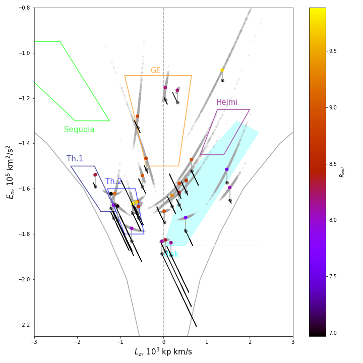
Figure 10: Comparison of the position in $E_{n}-L_{z}$ diagram calculated in axisymmetric (colored points with blue error bars) and non-axisymmetric (black tilted lines) potentials. $E_{n}-L_{z}$ diagram with the loci of the biggest known accretion events: Gaia-Enceladus/Sausage (GE) (orange), Helmi stream (purple), Sequoia (green), Thamnos 1, 2 (darkblue, blue); and disk (cyan).

For both potentials, we run simulations 1 Gyr long in time with step $\Delta t=0.1$ Myr. For non-axisymmetric potential, though, we did not calculate uncertainties since it is a highly time-consuming process.

6 Conclusions

Three main parameters that can be used to obtain the origin of the star are: kinematics, chemistry and age. In this study, we explored all three of them for a sample of 28 very metal-poor stars for whom we had previously derived ages ((Plotnikova et al., 2022)). Kinematics and chemistry are routinely used to assign stars to different components of the Milky Way galaxy, or to the various accreted systems that have been identified over the years in the Galactic halo. The basic conclusions of our study can be summarized as follows:

• We have identified a group of stars with clear signatures of Halo population according to their chemistry, age, and kinematics. However, we speculate that several of them, the oldest 8 indeed, could have formed in the primordial Bulge because of their orbital parameters (large eccentricity and low $Z_{max}$ mostly) and large $\alpha$-abundance.

• We have identified another group of stars that we tentatively associate with Gaia-Enceladus/Sausage (GE) (orange), and Thamnos 1, 2 (dark blue, blue) according to their similarity in kinematics, chemistry and age.

The identification of a group, although small, of stars probably belonging to the infant Bulge is rather intriguing. In fact, it supports a scenario in which the first component of the Milky Way to form was the Bulge via a fast collapse a là ELS (Eggen et al. (1962)). The other components have then assembled with a major contribution from systems that engulfed into the Milky Way later on, in agreement with the widely accepted merging scheme (Searle & Zinn (1978)).

References

- Bailer-Jones et al. (2021) Bailer-Jones, C. A. L., Rybizki, J., Fouesneau, M., Demleitner, M., & Andrae, R. 2021, AJ, 161, 147
- Barklem et al. (2005) Barklem, P. S., Christlieb, N., Beers, T. C., et al. 2005, A&A, 439, 129
- Belokurov et al. (2018) Belokurov, V., Erkal, D., Evans, N. W., Koposov, S. E., & Deason, A. J. 2018, MNRAS, 478, 611
- Bland-Hawthorn & Gerhard (2016) Bland-Hawthorn, J., & Gerhard, O. 2016, ARA&A, 54, 529
- Bovy (2015) Bovy, J. 2015, The Astrophysical Journal Supplement Series, 216, 29
- Bovy et al. (2019) Bovy, J., Leung, H. W., Hunt, J. A. S., et al. 2019, MNRAS, 490, 4740
- Bullock & Johnston (2005) Bullock, J. S., & Johnston, K. V. 2005, ApJ, 635, 931
- Carraro et al. (1999) Carraro, G., Girardi, L., & Chiosi, C. 1999, MNRAS, 309, 430
- Chemel et al. (2018) Chemel, A. A., Glushkova, E. V., Dambis, A. K., et al. 2018, Astrophysical Bulletin, 73, 162
- Clarke et al. (2019) Clarke, J. P., Wegg, C., Gerhard, O., et al. 2019, MNRAS, 489, 3519
- Courteau et al. (1996) Courteau, S., de Jong, R. S., & Broeils, A. H. 1996, ApJ, 457, L73
- Drimmel & Poggio (2018) Drimmel, R., & Poggio, E. 2018, Research Notes of the American Astronomical Society, 2, 210
- Eggen et al. (1962) Eggen, O. J., Lynden-Bell, D., & Sandage, A. R. 1962, ApJ, 136, 748
- François et al. (2007) François, P., Depagne, E., Hill, V., et al. 2007, A&A, 476, 935
- Fulbright (2000) Fulbright, J. P. 2000, AJ, 120, 1841
- Gadotti & dos Anjos (2001) Gadotti, D. A., & dos Anjos, S. 2001, AJ, 122, 1298
- Gaia Collaboration (2021) Gaia Collaboration. 2021, A&A, 649, A1
- Gaia Collaboration et al. (2022) Gaia Collaboration, Gaia Collaboration, De Ridder, J., et al. 2022, arXiv e-prints, arXiv:2206.06075
- GRAVITY Collaboration et al. (2018) GRAVITY Collaboration, Abuter, R., Amorim, A., et al. 2018, A&A, 615, L15
- Grenon (1985) Grenon, M. 1985, in Cool Stars with Excesses of Heavy Elements, ed. M. Jaschek & P. C. Keenan, Vol. 114, 147
- Grillmair (2017) Grillmair, C. J. 2017, ApJ, 847, 119
- Helmi (2002) Helmi, A. 2002, Ap&SS, 281, 351
- Helmi et al. (2018) Helmi, A., Babusiaux, C., Koppelman, H. H., et al. 2018, Nature, 563, 85
- Howes et al. (2016) Howes, L. M., Asplund, M., Keller, S. C., et al. 2016, MNRAS, 460, 884
- Ibata et al. (2002) Ibata, R. A., Lewis, G. F., Irwin, M. J., & Cambrésy, L. 2002, MNRAS, 332, 921
- Johnson et al. (2012) Johnson, C. I., Rich, R. M., Kobayashi, C., & Fulbright, J. P. 2012, ApJ, 749, 175
- Johnson et al. (2014) Johnson, C. I., Rich, R. M., Kobayashi, C., Kunder, A., & Koch, A. 2014, AJ, 148, 67
- Koppelman et al. (2019) Koppelman, H. H., Helmi, A., Massari, D., Price-Whelan, A. M., & Starkenburg, T. K. 2019, A&A, 631, L9
- Lindegren et al. (2021) Lindegren, L., Bastian, U., Biermann, M., et al. 2021, A&A, 649, A4
- Lucey et al. (2022) Lucey, M., Hawkins, K., Ness, M., et al. 2022, MNRAS, 509, 122
- McMillan (2017) McMillan, P. J. 2017, MNRAS, 465, 76
- Myeong et al. (2019) Myeong, G. C., Vasiliev, E., Iorio, G., Evans, N. W., & Belokurov, V. 2019, MNRAS, 488, 1235
- Nordlander & Lind (2017) Nordlander, T., & Lind, K. 2017, A&A, 607, A75
- Plotnikova et al. (2022) Plotnikova, A., Carraro, G., Villanova, S., & Ortolani, S. 2022, ApJ, 940, 159
- Portail et al. (2017) Portail, M., Gerhard, O., Wegg, C., & Ness, M. 2017, MNRAS, 465, 1621
- Portail et al. (2015) Portail, M., Wegg, C., Gerhard, O., & Martinez-Valpuesta, I. 2015, MNRAS, 448, 713
- Queiroz et al. (2019) Queiroz, A. B. A., Anders, F., Chiappini, C., et al. 2019, arXiv e-prints, arXiv:1912.09778
- Reddy et al. (2006) Reddy, B. E., Lambert, D. L., & Allende Prieto, C. 2006, MNRAS, 367, 1329
- Reddy et al. (2003) Reddy, B. E., Tomkin, J., Lambert, D. L., & Allende Prieto, C. 2003, MNRAS, 340, 304
- Reid & Brunthaler (2004) Reid, M. J., & Brunthaler, A. 2004, ApJ, 616, 872
- Roederer et al. (2014) Roederer, I. U., Preston, G. W., Thompson, I. B., et al. 2014, AJ, 147, 136
- Ruiz-Lara et al. (2022) Ruiz-Lara, T., Matsuno, T., Lövdal, S. S., et al. 2022, A&A, 665, A58
- Sanders et al. (2019) Sanders, J. L., Smith, L., Evans, N. W., & Lucas, P. 2019, MNRAS, 487, 5188
- Searle & Zinn (1978) Searle, L., & Zinn, R. 1978, ApJ, 225, 357
- Sestito et al. (2022) Sestito, F., Venn, K. A., Arentsen, A., et al. 2022, arXiv e-prints, arXiv:2208.13791
- Simmerer (2004) Simmerer, J. 2004, in American Astronomical Society Meeting Abstracts, Vol. 205, American Astronomical Society Meeting Abstracts, 77.05
- Sormani et al. (2015) Sormani, M. C., Binney, J., & Magorrian, J. 2015, MNRAS, 454, 1818
- Tkachenko et al. (2023) Tkachenko, R., Korchagin, V., Jmailova, A., Carraro, G., & Jmailov, B. 2023, Galaxies, 11, 26
- VandenBerg et al. (2014) VandenBerg, D. A., Bond, H. E., Nelan, E. P., et al. 2014, ApJ, 792, 110
- Wegg & Gerhard (2013) Wegg, C., & Gerhard, O. 2013, MNRAS, 435, 1874
- Yeh et al. (2020) Yeh, F.-C., Carraro, G., Korchagin, V. I., Pianta, C., & Ortolani, S. 2020, A&A, 635, A125
- Yong et al. (2013) Yong, D., Norris, J. E., Bessell, M. S., et al. 2013, ApJ, 762, 26
- Yuan et al. (2020) Yuan, Z., Myeong, G. C., Beers, T. C., et al. 2020, ApJ, 891, 39