Ultra-High-Resolution Detector Simulation with Intra-Event Aware GAN and Self-Supervised Relational Reasoning

Abstract

Simulating high-resolution detector responses is a storage-costly and computationally intensive process that has long been challenging in particle physics. Despite the ability of deep generative models to make this process more cost-efficient, ultra-high-resolution detector simulation still proves to be difficult as it contains correlated and fine-grained mutual information within an event. To overcome these limitations, we propose Intra-Event Aware GAN (IEA-GAN), a novel fusion of Self-Supervised Learning and Generative Adversarial Networks. IEA-GAN presents a Relational Reasoning Module that approximates the concept of an ”event” in detector simulation, allowing for the generation of correlated layer-dependent contextualized images for high-resolution detector responses with a proper relational inductive bias. IEA-GAN also introduces a new intra-event aware loss and a Uniformity loss, resulting in significant enhancements to image fidelity and diversity. We demonstrate IEA-GAN’s application in generating sensor-dependent images for the high-granularity Pixel Vertex Detector (PXD), with more than 7.5M information channels and a non-trivial geometry, at the Belle II Experiment. Applications of this work include controllable simulation-based inference and event generation, high-granularity detector simulation such as at the HL-LHC (High Luminosity LHC), and fine-grained density estimation and sampling. To the best of our knowledge, IEA-GAN is the first algorithm for faithful ultra-high-resolution detector simulation with event-based reasoning.

Keywords High-resolution and high-granularity detector simulation  $\cdot$ Fine-grained conditional image generation  $\cdot$ Relational Inductive Bias  $\cdot$ GANs  $\cdot$ Self-Supervised Learning with Knowledge Transfer

1 Introduction

The “Fast and Efficient Simulation” [1, 2, 3, 4, 5, 6, 7, 8, 9, 10, 11, 12] campaign in particle physics sparked the search for faster and more storage-efficient simulation methods of collider physics experiments. Simulations play a vital role in various downstream tasks, including optimizing detector geometries, designing physics analyses, and searching for new phenomena beyond the Standard Model (SM). Efficient detector simulation has been revolutionized by the introduction of the Generative Adversarial Network (GAN) [13] for image data.

GANs have been widely used in particle physics to achieve detector simulation for the LHC [14, 15, 16], mainly targeting calorimeter simulation or collision event generation [17, 18, 19]. Previous work on generating high spatial resolution detector responses includes the Prior-Embedding GAN (PE-GAN) by Hashemi. et al. [20], which utilizes an end-to-end embedding of global prior information about the detector sensors, and the work by Srebre et al. [21] in which a Wasserstein GAN [22] with gradient penalty [23] was used as a proof of concept to generate high resolution images without conditioning. For mid-granularity calorimeter simulation, the recent approaches [24, 25], experiment with several GAN-like and normalizing flow [26] architectures with less that 30k simulated channels, and 3DGAN [16] for high granularity calorimeter simulation with only 65k pixel channels.

The task of learning to generate ultra-high resolution detector responses has several challenges. First, in general we are dealing with spatially asymmetric high-frequency hitmaps. With current state of the art (SOTA) GAN setups for high-resolution image generation candidates, when the discriminator becomes much stronger than the generator, the fake images are easily separated from real ones, thus reaching a point where gradients from the discriminator vanish. This happens more frequently with asymmetric high-resolution images due to the difficulty of generating imbalanced high-frequency details. On the other hand, a less powerful discriminator results in a mode collapse, where the generator greedily optimizes its loss function producing only a few modes to deceive the discriminator.

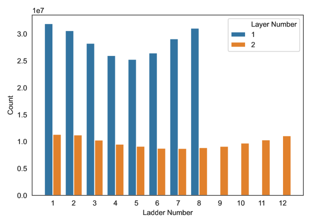
Figure 8: The number of PXD hits per layer and sensor (ladder). Each sensor has different occupancies for sensors in the inner and outer layers. The global asymmetry between them stems from the $\phi$ dependency of PXD images.

Furthermore, the detector responses in an event, a single readout window after the collision of particles, share both statistical and semantic similarities [27] with each other. For example, the sparsity (occupancy) of each image within a class, defined as the fraction of pixels with a non-zero value, shows statistical similarities between detector components as shown in Figure 8. Moreover, as the detector response images show extreme resemblance at the semantic and visual levels [27], they can be classified as fine-grained images. When generating fine-grained images, the objective is to create visual objects from subordinate categories. A similar scenario in computer vision is generating images of different dog breeds or car models. The small inter-class and considerable intra-class variation inherent to fine-grained image analysis make it a challenging problem [28]. The current state-of-the-art conditional GAN models focus on class and intra-class level image similarity, in which intra-image [29], data-to-class [30], and data-to-data [31] relations are considered. However, in the case of detector simulation, classes become hierarchical and fine-grained, and the discrimination between generated classes that are semantically and visually similar becomes harder. Therefore, the aforementioned models show extensive class confusion [32, 33] at the inter-class level. In addition, since the information in an event comes from a single readout window of the detector, the processes happening in this window affect all sensors simultaneously, leading to a correlation among them, as shown in Figure 3.

To overcome all these challenges with high-resolution detector simulation, we introduce the Intra-Event Aware GAN (IEA-GAN), a new model to generate sensor/layer-dependent detector response images with the highest fidelity while satisfying all relevant metrics. Since we are dealing with a fine-grained and contextualized (by each event) set of images that share information, first, we introduce a Relational Reasoning Module (RRM) for the discriminator and generator to capture inter-class relations. Then, we propose a novel loss function for the generator to imitate the discriminator’s knowledge of dyadic class-to-class correspondence [34]. Finally, we introduce an auxiliary loss function for the discriminator to leverage its reasoning codomain by imposing a information uniformity condition [35] to alleviate mode-collapse issue and increase the generalization of the model. IEA-GAN captures not only statistical-level and semantic-level information but also a correlation among samples in a fine-grained image generation task.

We demonstrate the IEA-GAN’s application on the ultra-high dimensional data of the Pixel Vertex Detector (PXD) [36] at Belle II [37] with more than 7.5M pixel channels- the highest spatial resolution detector simulation dataset ever analyzed with deep generative models. Then, we investigate several evaluation metrics and show that in all of them IEA-GAN is in much better agreement with the target distribution than other SOTA deep generative models for high-dimensional image generation. We also perform an ablation study and exploration of hyperparameters to provide insight to the model. In the end, by applying IEA-GAN to the PXD at Belle II we are able to reduce the storage demand for pre-produced background data by a factor of $2$.

2 Results

2.1 IEA-GAN Architecture

IEA-GAN is a deep generative model based on a self-supervised relational grounding. A GAN is an unsupervised deep learning architecture that involves two networks, the Generator and the Discriminator, whose goal is to find a Nash equilibrium [38] in a two-player min-max problem.

IEA-GAN’s discriminator, $D$, takes the set of detector response images $x_{i}\in\mathbf{R}^{d}$ coming from one event and embeds them as input nodes within a fully connected event graph in a self-supervised way. It approximates the concept of an event by contextual reasoning using the a permutation equivariant Relational Reasoning Module (RRM). RRM is a novel, GAN-compatible, fully connected, multi-head Graph Transformer Network [39, 40, 41] that groups the image tokens in an event based on their contextual similarity. For multi-modal contrastive reasoning, the discriminator also takes the sensor embedding of the detector as class tokens (see section 4). In the end, it compactifies both image and class modalities information by projecting the normalized graph onto a hypersphere, as shown in Figure 1(a).

To ensure that the Generator $G$ has a proper understanding of an event and captures the intra-event correlation, it first samples from a Normal distribution, $\mathcal{N}(0,1)$, at each event as random degrees of freedom (Rdof), and decorates the sensor embeddings with this four-dimensional learnable Rdof (see section 4). Then, for a self-supervised contextual embedding of each event, the RRM acts on top of this. Notably, Rdof differs from the original GAN [13] Gaussian latent vectors. Rdof can be considered a event-level learnable segment embedding [42] and perturbation [43] to the token embeddings, which can leverage the diversity of generated images. Combining these modules with the IEA Loss allows the Generator to gain insight and establish correlation among the samples in an event, thus improving its overall performance.

Apart from the adversarial loss, IEA-GAN also benefits from self-supervised and contrastive-based set of losses. The model understands the geometry of detector through a proxy-based contrastive 2C loss [31] where the learnable proxies are the sensor embeddings over the hypersphere. Moreover, to improve diversity and stability of the training, we introduce a Uniformity loss for the discriminator. The uniformity loss can encourage the discriminator to give equal weight to all regions of the hypersphere [35], rather than just focusing on the areas where it can easily distinguish between real and fake data. Encouraging the discriminator to impose uniformity not only promotes more diverse and varied outputs, but also mitigates issues such as mode collapse.

Another essential part of IEA-GAN is the IEA loss that addresses the class-confusion [32, 33] problem of the conditional generative models for fine-grained datasets. In the IEA-loss the generator tries to imitate the discriminator’s understanding of each event through a dyadic information transfer with a stop-gradient for the discriminator. This can improve the ability of the generator to generate more fine-grained samples in the simulation process by being aware of the variability of conditions at each event.

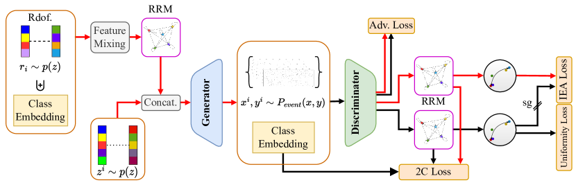
(a) Rdof stands for Random degrees of freedom, which decorates the generator’s sensor/layer embedding with an event-level learnable embedding responsible for the generator’s intra-event correlation. The Relational Reasoning Modules (RRM) in the generator and the discriminator do the intra-event reasoning by clustering class/image embeddings based on their contextual similarity, respectively. The red lines correspond to the forward and backward passes of the generator. The black lines correspond to the forward and backward passes of the discriminator. The discriminator is trained with the Adversarial loss, see eq. 2, 2C loss, see eq. 3 and the Uniformity loss, see eq. 12. On the other hand, the generator uses the Adversarial loss, 2C loss, and the IEA loss, see eq. 11. Sg means stop-gradient for the discriminator from the IEA loss, a self-supervised dyadic-aware loss for the generator.

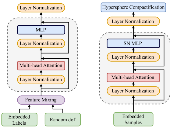
(b) The Relational Reasoning Module for the generator (left) and the discriminator (right)

Figure 1: IEA-GAN architecture (a) and Relational Reasoning Module components (b). SN stands for spectrally normalized layers that only the discriminator incorporates.

2.2 IEA-GAN Evaluation

Our study showcases the performance of IEA-GAN in generating high-resolution detector responses, demonstrated through its successful application to the ultra-high dimensional data of the Pixel Vertex Detector (PXD) at Belle II, consisting of over 7.5 million pixel channels. Furthermore, for the first time, our findings reveal that the FID [44] metric for detector simulation is a very versatile and accurate unbiased estimator in comparison to marginal distributions, and is correlated with both high and low level metrics. We show that by using IEA-GAN, we are able to capture the underlying distributions such that we can generate and amplify detector response information with a very good agreement with the Geant4 distributions. We also find out that the SOTA models in high resolution image generation even with an in-depth hyperparameter tuning analysis do not perform well in comparison.

For evaluation, we have two categories of metrics: image level and physics level. As we are interested in having the best pixel-level properties, diversity, and correlation of the generated images simultaneously while adhering to minimal generator complexity due to computational limitations, choosing the best iteration to compare results is challenging. Hence, we choose models’ weights with the best FID for all comparisons. Based on the recent Clean-FID project [45], we fine-tune the Inception-V3 [46] model on the PXD images, as the PXD images are very different from the natural images used in their initial training. This process can be done for any other detector dataset. FID measures the similarity of the generated samples’ representations to those of samples from the real distribution. Given a large sampling statistics, for each hidden activation of the Inception model, the FID fits a Gaussian distribution and then evaluates the Fréchet distance, also known as Wasserstein-2 distance, between those Gaussians. The lower the FID score, the more similar the distributions of the real and generated samples are.

We compare IEA-GAN with three other models and the reference, which is the Geant4-simulated [47] dataset. The baselines are the SOTA in conditional image generation: BigGAN-deep [48] and ContraGAN [31]. We also compare IEA-GAN with the previous works on PXD image generation task: PE-GAN [20] and WGAN-gp [21].

Table 1 demonstrates that generated images by IEA-GAN have the lowest FID score compared to the other models and outperforms them by a significant margin. This indicates that our model is able to generate synthetic samples that are much closer to the target data than the samples generated by the other models.

Table 1: FID comparison between models (all models in the benchmark are highly tuned to the current problem and dataset), averaged across six random seeds. The lower the FID the better the image quality and diversity.

	WGAN-gp	BigGAN-deep	ContraGAN	PE-GAN	IEA-GAN
FID	$12.09$	$4.40\pm 0.88$	$3.14\pm 0.74$	$2.61\pm 0.91$	$\mathbf{1.50\pm 0.16}$

At the pixel level, there are the pixel intensity distribution, occupancy distribution, and mean occupancy. The pixel intensity distribution defines the distribution of the energy of the background hits. The occupancy distribution and the pixel intensity distribution are evaluated over all sensors of a given number of events, while the mean occupancy corresponds to the mean value of sparsity across events for each sensor. This pixel-level information is essential since upon physics analysis via the basf2 software [49], when one wants to use the images and overlay the extracted information on the signal hits, the sparsity of the image defines the volume of the background hits on each sensor. The pixel intensity distribution, the occupancy distribution, as well as the mean occupancy per sensor are shown in Figure 2. The distributions for the IEA-GAN model show the closest agreement with the reference.

The bimodal distribution of the occupancy comes from the geometry of the detector as the sensors are not in a cylindrical shape like a calorimeter, but in an annulus shape. This indicates how challenging simulating this dataset is concerning both it’s geometry and resolution. In order to capture the correct bi-modality of the occupancy distribution, RRM and the Uniformity loss play an important role. By using a uniformity loss in the discriminator, the generator is incentivized to produce samples that are not biased towards a particular mode or class, leading to a wider bimodal distribution of generated samples.

Moreover, by utilizing the RRM module that considers the inter-dependencies and correlations among the samples within an event, the IEA-GAN exhibits a superior consistency with high-energy hits, which enhances the diversity of generated samples in regions with lower occurrence rates.

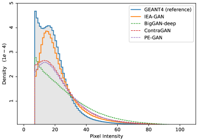
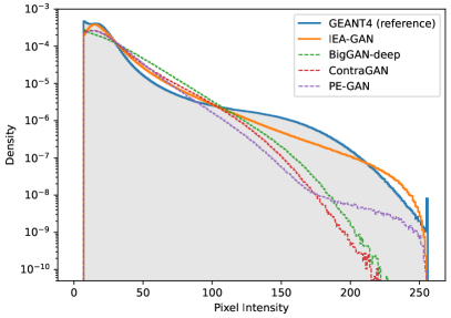
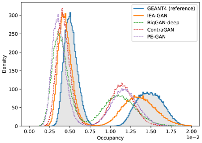
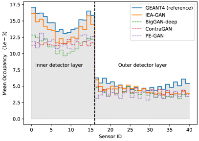
Figure 2: Pixel intensity distribution in linear (top left) and logarithmic scale (top right), the distribution of the occupancy (bottom left) and the mean occupancy per sensor (bottom right) for $10\,000$ events.

Along with all these image-level metrics, we also need an intra-event sensitive metric. All the above metrics are equivariant under permutation between the samples among events. In other words, if we randomly shuffle the samples between events while fixing the sensor number, all the discussed metrics are unchanged. Hence, we need a metric that looks at the context of each event individually in its event space and goes beyond the sample space. Ergo, we compute the Spearman’s correlation between the occupancy of the sensors along the population of generated events,

$$r_{s}=\mathbf{Corr_{p}}(R(\biguplus_{i=1}^{M=40}(\|x_{i}\|_{0})),R(\biguplus_{i=1}^{M=40}(\|x_{i}\|_{0}))),$$

where $R(.)$ is the rank variable, and $\mathbf{Corr_{p}}(.)$ is the Pearson Correlation function. The coefficients by PE-GAN are random values in the range $[-0.2,0.2]$, whereas IEA-GAN images show a meaningful correlation among their generated images. Even though the desired correlation is different from the reference, as shown in Figure 3, IEA-GAN understands a monotonically positive correlation for intra-layer sensors and a primarily negative correlation for inter-layer sensors.

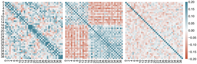
Figure 3: Spearman’s correlation between the occupancy of Geant4 sensor images (left), and sensor images from IEA-GAN (center), sensor images from PE-GAN (right).

While image level metrics indicate the low-level quality of simulations, we must also confirm that the resulting simulations are reasonable physics-wise when the entire detector is considered as a whole. For this, we examine the Helix Parameter Resolution (HPR). At the Belle II experiment, after each collision event, tracks propagating in vacuum in a uniform magnetic field move roughly along a helix path described by the five helix parameters $\{d_{0},z_{0},\phi_{0},\omega,\tan\lambda\}$ with respect to a pivot point [50]. The difference between the true and reconstructed helix parameters defines the resolution for the corresponding helix parameter. The track parameter resolution is affected by the number of hits and the hit intensity. The resolutions of all five helix parameters are shown in Figure 4 for $5000$ events. We observe good agreement between the IEA-GAN and Geant4, particularly in the tail segments where the largest difference between Geant4 and no background is found. Hence, not only does IEA-GAN demonstrate a close image level agreement with Geant4, it maintains a reconstructed physical behavior during track reconstruction as well.

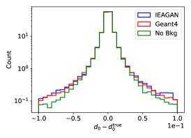
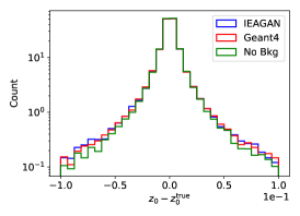
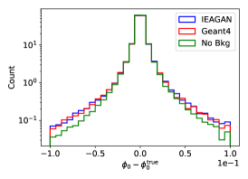
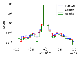
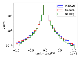
Figure 4: Helix parameter resolutions for $d_{0}$ (top left), $z_{0}$ (top middle), $\phi_{0}$ (top right), $\omega_{0}$ (bottom left), and $\tan\lambda$ (bottom right). Blue corresponds to the IEA-GAN simulated background, red to Geant4, and green to resolution with no background overlay.

3 Discussion

In this work, we have proposed a series of robust methods for ultra-high-resolution, fine-grained, correlated detector response generation and conditional sampling tasks with our Intra-Event Aware GAN (IEA-GAN). IEA-GAN not only captures the dyadic class-to-class relations but also exhibits explainable intra-event correlations among the generated detector images while other models fail to capture any correlation. To achieve this, we present novel components, the Relational Reasoning Module (RRM) and the IEA-loss, with the Uniformity loss [35], used in Deep Metric Learning. The RRM introduced a self-supervised relational contextual embedding for the samples in an event, which is compatible with GAN training policies, a task that is very challenging. It dynamically clusters the images in a collider event based on their inherent correlation culminating in approximating a collision event. Our IEA-loss, a discriminator-supervised loss, helps the generator reach a consensus over the discriminator’s dyadic relations between samples in each event. Finally, we have demonstrated that the Uniformity loss plays a crucial role for the discriminator in maximizing the homogeneity of the information entropy over the embedding space, thus helping the model to overcome mode-collapse and to capture a better bi-modality of generated occupancy.

As a result, an improvement to all metrics compared to the previous SOTA occurs, achieving an FID score of $1.50$, an over $42\%$ improvement, and a storage release of more than $2$ orders of magnitude. Moreover, we have showed that the application of the FID metric, an unbiased estimator, for the detector simulation provides a powerful tool for evaluating the performance of deep generative models in detector simulation. We have also conducted an in-depth study into the optimal design and hyperparameters of the RRM, the IEA-loss, and the Uniformity loss.

Table 2: Computational performance of IEA-GAN and PE-GAN generators on a single core of an Intel Xeon Silver $4108$ $1.80$GHz (CPU) and NVIDIA V100 with $32$ GB of memory (GPU) compared to GEANT4. For the generative models, the mean and standard deviation were obtained for sets of $10\,000$ events. The time for GEANT4 refers to the theoretical time it would take to run the simulation of all background processes on-the-fly. The storage consumption corresponds only to $1$ times the PXD background simulated information where the amplification coefficient $N$ is equal to $1$.

Hardware	Simulator	time/event [s]	storage [Mb]
CPU	Geant4	$\approx 1500$	$\approx 2000$
	PE-GAN	$11.781\pm 0.357$	$\approx 47$
	IEA-GAN	$10.159\pm 0.208$	$\approx 47$
GPU	PE-GAN	$0.090\pm 0.010$	$\approx 47$
	IEA-GAN	$0.070\pm 0.006$	$\approx 47$

The ability to capture the underlying correlation structure of the data in particle physics experiments where the physical interpretation of the results heavily relies on it, is very important. The true correlation between the occupancy of the sensors is determined by the underlying physical processes within the simulation. Although the true correlation differs from the one captured by IEA-GAN, the model might be learning biases or artifacts introduced by the training data or the discriminator. Therefore, while the IEA-GAN can provide valuable insights into the correlations and patterns present in the data, it is important to interpret its results in conjunction with the domain knowledge. To alleviate the discrepancy, we expect that incorporating perturbations directly to the discriminator’s RRM module would improve its contextual understanding and thus the intra-event correlation. For example, using random masking [51] or inter-event permutation [52] over the samples and asking the RRM module to predict the representation of perturbed sample will improve the robustness of the model.

This work has a significant impact on high-resolution fast and efficient detector response and collider event simulations. Since, they require fine-grained intra-event-correlated data generation, we believe that the Intra-Event Aware GAN (IEA-GAN) offers a robust controllable sampling for all particle physics experiments and simulations, such as detector simulation [16, 53] and event generation [18, 54, 55, 56] at both Belle II [37] and LHC [57]. In particular, the High-Luminosity Large Hadron Collider (HL-LHC) [58] is expected to surpass the LHC’s design integrated luminosity by increasing it by a factor of 10. As a result, more effective and efficient high-resolution detector simulations are required. IEA-GAN is the first potential candidate for simulating the corresponding high-resolution and high-granular detector signatures with the remarkable capability of generating more than 7.5M pixel channels.

Finally, IEA-GAN also has potential applications in the protein design which is a process that involves the generation of novel amino acid sequences to produce proteins with desired functions, such as enhanced stability and foldability, new binding specificity, or enzymatic activity [59]. Proteins can be grouped into different categories based on the arrangement and connectivity of their secondary structure features, such as alpha helices and beta sheets. Our developed intra-event aware methods, where an event represents the higher category of features, can also be applied to fine-grained density estimation [60] for generating novel foldable protein [61, 62, 63] structures where category-level reasoning is of paramount importance.

4 Methods

4.1 Dataset

In this paper, we study the most challenging detector simulation problem with the highest spatial resolution dataset coming from the Pixel Vertex Detector (PXD) [36], shown in Figure 5(a), the innermost sub-detector of Belle II [37]. The configuration of the PXD consists of $40$ sensors within two detector layers, as shown in Figure 5(b). The inner layer has $16$ sensors, and the outer layer comprises $24$ sensors. Thus, each event includes $40$ grey-scale images, each with a resolution of $250\times 768$ pixels, resulting in more than 7.5 million pixel channels per event as shown in Figure 5(c).

The problem with such a high-resolution background overlay [64] is that many resources are required for their readout, storage, and distribution. For example, the size of the PXD background overlay data needed for the simulation of a single event is approximately $200\text{\,}\mathrm{k}$B. This is roughly $2$ times the size of the background overlay data per event with respect to all other detector components together [65]. While storing such a massive amount of data is very inefficient for high-resolution detectors, we propose to generate them with IEA-GAN on the fly, which will free up a significant amount of storage space (see Table 2 in appendix B). In this way, the only storage cost is for the weights of the IEA-GAN, depicted in Figure 5(d).

For training and evaluation, we used $40\,000$ and $10\,000$ Monte Carlo simulated [65] events, respectively. The data in each event consists of $40$ grey-scale $256\times 768$ zero-padded images. They are zero-padded on both sides from their original size of $250\times 768$ to be divisible by $16$ for training purposes.

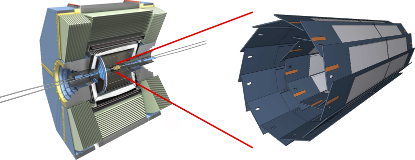
(a)

(b)

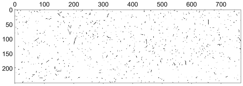
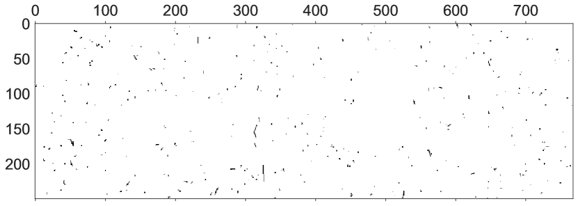
(c)

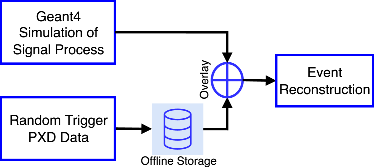
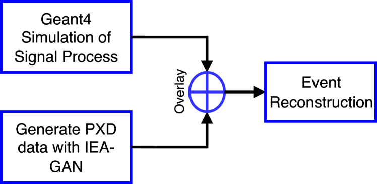
(d)

Figure 5: Pixel detector layout The pixel detector (PXD) is the inner-most sub-detector of the Belle II experiment (a) and is configured in a two-layered overlapping sensor structure (b). PXD image examples (c) for sensors $7$ (top) and $25$ (down). (d) The event generation pipeline with Geant4 [47] (top) and using IEA-GAN (bottom). Generating PXD data on the fly of analysis avoids the need to store them offline.

4.2 Theory of Generative adversarial Networks

GANs are generative models that try to learn to generate the input distribution as faithfully as possible. For conditional GANs [66], the goal is to generate features given a label. Two player-based GAN models introduce a zero-sum game between two Synthetic Intelligent Agents, a generator network $G$, and a discriminator network $D$.

Definition 4.1 (Vanilla GAN).

Given the generator $G$, a function $G:\mathbb{R}^{d}\rightarrow\mathbb{R}^{n}$, that maps a latent variable $z\in\mathbb{R}^{d}$ sampled from a distribution to an n-dimensional observable, and the discriminator $D$, a functional $D:\mathbb{R}^{n}\rightarrow[0,1]$, that takes a generated image $x\in\mathbb{R}^{n}$ and assigns a probability to it, they are the players of the following two-player minimax game with value function $V(D,G)$ [13],

$$\mathop{min}_{G}\mathop{max}_{D}~{}V(D,G)=\mathbb{E}_{x\in\mathbb{R}^{n}}[\log D(x)]+\mathbb{E}_{z\in\mathbb{R}^{d}}[\log(1-D(G(z))].$$

After introducing the vanilla GAN, a vast amount of research has been undertaken to improve its convergence and stability, as, in general, training GANs is a highly brittle task. It requires a significant amount of hyperparameter tuning for domain-specific tasks. Many tricks, model add-ons, and structural changes have been introduced. A recent and comprehensive study prompted a very powerful SOTA model, BigGAN-deep [48], which incorporates the hinge-loss variation of the adversarial loss [67],

$$\pazocal{L}_{D}^{\mathrm{hinge}} =-\mathbb{E}_{x\in\mathbb{R}^{n}}[\min(0,-1+D(x))]-\mathbb{E}_{z\in\mathbb{R}^{d}}[\min(0,-1-D(G(z))]~{},$$ (1)

$$\pazocal{L}_{G}^{\mathrm{hinge}} =-\mathbb{E}_{z\in\mathbb{R}^{d}}[D(G(z))].$$ (2)

Furthermore, many schemes for capturing the class conditions have been proposed since conditional GANs over image labels have been introduced [66]. The main idea is to minimize a specific metric between a class identification output of the discriminator and the actual labels after injecting an embedding of the conditional prior information to the generator. For example, ACGAN [68] tries to capture data-to-class relations by introducing an auxiliary classifier. The ProjGAN [30] also tries to capture these data-to-class relations by projecting the class embeddings onto the output of the discriminator via an inner product that contributes to the adversarial loss. The recent ContraGAN [31] incorporated concepts from metric learning or self-supervised learning (SSL) in order to seize data-to-data relations or intra-class relations by introducing the 2C loss, derived from NT-Xent loss [69], and proxy-based SSL,

Here, $x_{i}$ are the images, $y_{i}$ are the corresponding labels, $S_{c}(.,.)$ is a similarity metric, and $h(.)$ is the output of the image embeddings. Although ContraGAN benefits from this loss by capturing the intra-class characteristics among the images that belong to the same class, it is prone to class-confusion [32, 33] as different classes could also show similarity among themselves since their vector representation in the embedding space might not be orthogonal to each other, which is precisely what we are dealing with in a fine-grained dataset.

4.3 Relational Reasoning

4.3.1 Background

Transformers [70] are widely used in different contexts. However, their application in Generative Adversarial Networks is either over the image manifold to learn long-range interactions between pixels [29, 71] or via pure Vision-Transformer based GANs [72] in which they utilize a fully Vision-Transformer [73] based generator and discriminator. Given the fact that training the Transformers is notoriously difficult [74] and task-agnostic when determining the best learning rate schedule, warm-up strategy, decay settings, and gradient clipping, fusing and adapting a Transformer encoder over a GAN learning regime is a highly non-trivial task. In this paper, we successfully merge a Transformer-based module adapted to the GAN training schemes for the discriminator’s image and the generator’s class modalities without any of the aforementioned problems.

Definition 4.2 (Attention).

Transformers utilize a self-attention mechanism, the data of $(K,Q,V,A)$. The vector spaces $K\in\mathbb{R}^{N\times d_{k}}$, $Q\in\mathbb{R}^{N\times d_{k}}$ and $V\in\mathbb{R}^{N\times d_{v}}$ are the set of Keys, Queries, and Values. The bilinear map $a:K\times Q\rightarrow\mathbb{R}^{N\times N}$ is a similarity function between a key and a query. The attention, $A$, is defined as

$$A(K,Q,V):=\mathrm{softmax}(a(K,Q))V~{},$$

where $d_{k}$ and $d_{v}$ are the dimensions of the corresponding vector spaces.

The attention mapping used in the vanilla Transformer [70] adopts the scaled dot-product as the bilinear map between keys and queries as

$$A(K,Q,V):=\mathrm{softmax}(\frac{KQ^{T}}{\sqrt{d_{k}}}))V~{}.$$ (4)

The normalization factor $\frac{1}{\sqrt{d_{k}}}$ mitigates vanishing gradients for large inputs. Rather than simply computing the attention once, the multi-head mechanism runs through the scaled dot-product attention of linearly transformed versions of keys, queries, and values multiple times in parallel via learnable maps $W_{i}^{k}$, $W_{i}^{q}$ and $W_{i}^{v}$. The independent attention outputs over $h$ number of heads are then aggregated and projected back into the desired number of dimensions via $W^{p}$,

$$\mathrm{MultiHead}(K,Q,V):=[\biguplus_{i=1}^{h}H_{i}]W^{p}~{},$$ (5)

where $H_{i}$ is given by $A(KW_{i}^{k},QW_{i}^{q},VW_{i}^{v})$. When used for processing sequences of tokens, the Self-Attention mechanism allows the transformer to figure out how important all other tokens in the sequence are, with respect to the target token, and then use these weights to build features of each token.

4.3.2 Event Approximation

Performing attention on all token pairs in a set to identify which pairs are the most interesting enables Transformers like Bert [42] to learn a context-specific syntax as the different heads in the multi-head attention might be looking at different syntactic properties [75, 76]. Therefore, to model the context-based similarity between the different detector sensors in each event rather than their absolute properties, we have to use a permutation-equivariant [77, 78] block such that it can encode pairwise correspondence among elements in the input set. For instance, Max-Pooling (e.g. DeepSets [79]) and Self-Attention [70] are the common permutation equivariant modules for set-based problems.

Moreover, it is impossible to pre-define meaningful sparse connections among the sample nodes in an event. For instance, the relation between images from different sensors can vary from event to event, albeit cumulatively, they follow a particular distribution. Hence, we use a self-attention mechanism with weighted sum pooling as a form of information routing to process meaningful connections between elements in the input set and create an event graph.

Each sample in an event is viewed as a node in a fully connected event graph, where the edges represent the learnable degree of similarity, as shown in Figure 1(a). Samples in each event go into message propagation steps of our Relational Reasoning Module (RRM), a GAN-compatible fully connected multi-head Graph Transformer Network [39, 40, 41].

4.3.3 Relational Reasoning Module

Specifically designed to be compatible with GAN training policies, the Relational Reasoning Module (RRM) can capture contextualized embeddings and cluster the image or class tokens in an event based on their inherent similarity.

Let $\mathbf{X}=\{x_{1},...,x_{m}\}$ be the set of the sampled images in each event, where $x_{i}\in\mathbb{R}^{d}$, and $\mathbf{y}=\{y_{1},...,y_{m}\}$ be the set of labels, with $y_{i}\in[\![1,40]\!]$ for $40$ detector (PXD) sensors. We also define two linear hypersphere projection diffeomorphisms, $\mathbf{h}_{x}:\mathbb{R}^{k}\rightarrow\mathbb{S}^{n}$ and $\mathbf{h}_{y}:\mathbb{Z}\rightarrow\mathbb{S}^{n}$, which map the image embedding manifold and the set of labels to a unit n-sphere, respectively. The unit n-sphere is the set of points, $\mathbb{S}^{n}=\{s\in\mathbb{R}^{n+1}\mid\|s\|_{2}=1\}$, that is always convex and connected. The Relational Reasoning Module benefits from a variant of the Pre-Norm Transformer [70] with a dot-product Multi-head Attention block such that

$$\mathbf{p}^{\prime(l)}_{i} =\mathbf{p}^{(l)}_{i}+\sum_{k=1}^{h}\sum_{j=1}^{m}a_{ij}^{(l,k)}\mathbf{W}_{\mathrm{SN}}^{(l)}\mathbf{LN}(\mathbf{p}_{j}^{(l)})~{},$$ (6)

$$\mathbf{p}^{(L)}_{i} =\mathbf{h}_{x}^{\mathrm{LN}}\left(\mathbf{LN}(\mathbf{\bigcirc}_{l=0}^{L}(\mathbf{p}^{\prime(l)}_{i}+\mathcal{F}_{\mathrm{SN}}[\mathbf{LN}(\mathbf{p}^{\prime(l)}_{i})]))\right)~{},$$ (7)

where $\mathbf{p}^{\prime(l)}_{i}\in\mathbb{R}^{k}$ is the embedding of each image via the discriminator for layer $l$ of the RRM. $\mathbf{LN}$ is the Layer Norm function [80] and $h$ is the number of heads defined in Equation 5. $\mathcal{F}[~{}.~{}]$ is a two layer MLP functional defined as $\mathcal{F}_{\mathrm{SN}}[\mathbf{p}_{i}^{(l)}]=\textrm{ReLU}(p_{i}^{(l)}\mathbf{W}_{\mathrm{SN}}^{(l,1)})\mathbf{W}_{\mathrm{SN}}^{(l,2)}$ with Spectral Normalization [81]. The logits $a_{ij}^{(l,k)}$ are the normalized Attention weights of the bilinear function that monitor the dyadic interaction between image embeddings in layer $l$ and head $k$ defined in Equation 4. $\mathbf{W}_{\mathrm{SN}}^{(l)}$ in Equation 6 is the learnable multi-head projector at layer $l$ defined in Equation 5 with Spectral Normalization. The output of the composition of all layers via the composition of $L$ functionals, $\bigcirc_{l=0}^{L}\Phi^{l}:=\phi_{w_{L}}\circ...\circ\phi_{w_{0}}[\mathbf{p}_{i}^{(l=0)}]\in\mathbb{R}^{m\times k}$, goes into a Layer Normalization layer where $\Phi^{l}=\mathbf{p}^{\prime(l)}_{i}+\mathcal{F}[\mathbf{LN}(\mathbf{p}^{\prime(l)}_{i})]$. $\mathbf{h}_{x}^{\mathrm{LN}}(~{}.~{})$ in Equation 7 is the hypersphere compactification while the vectors are being standardized over the unit n-sphere $\mathbb{S}^{n}$ by a Layer Normalization.

For the discriminator, this module takes the set of image embeddings as input nodes within a fully connected event graph, applies a dot-product self-attention over them, then updates each sample or node’s embedding via the attentive message passing, as shown on the right of Figure 1(b). In the end, it compactifies the information by projecting the normalized graph onto a hypersphere, as shown in Figure 1(a). Embedding the samples in an event on the unit hypersphere provides several benefits. In modern machine learning tasks such as face verification and face recognition [82], when dot products are omnipresent, fixed-norm vectors are known to increase training stability. In our case, this avoids gradient explosion in the discriminator. Furthermore, as $S^{n}$ is homeomorphic to the 1-point compactification of $\mathbb{R}^{n}$ when classes are densely grouped on the n-sphere as a compact convex manifold, they are linearly separable, which is not the case for the Euclidean space [83].

For the generator’s RRM, we use a simpler version of the above dot-product Multi-head Attention block without the last hypersphere compactification due to the stability issues., as shown on the left of Figure 1(b). It finds a learnable contextual embedding for each event that will be fused to each class token via the feature mixing layer, which is a matrix factorization linear layer $\mathbf{W}_{\mathrm{SN}}(.)$. Formally we have,

$$\mathbf{q}^{(0)}_{i} =\mathbf{W}_{\mathrm{SN}}(\mathbf{r}_{i}\uplus\mathbf{e}_{i})~{},$$ (8)

$$\mathbf{q}^{\prime(l)}_{i} =\mathbf{q}^{(l)}_{i}+\sum_{k=1}^{M}\sum_{j=1}^{m}a_{ij}^{(l,k)}\mathbf{W}^{(l)}\mathbf{LN}(\mathbf{q}_{j}^{(l)})~{},$$ (9)

$$\mathbf{q}^{L}_{i} =\mathbf{LN}\left(\mathbf{\bigcirc}_{l=0}^{L}(\mathbf{q}^{\prime(l)}_{i}+\mathcal{F}[\mathbf{LN}(\mathbf{q}^{\prime(l)}_{i})])\right)~{},$$ (10)

where $\mathbf{e}_{i}:\mathbb{Z}\rightarrow\mathbb{R}^{t}$ is the embedding of each class token via the embedding layer of the generator. The logits $a_{ij}^{(l,k)}$ are the normalized Attention weights of the bilinear function that monitor the dyadic interaction between classes in the event embeddings in layer $l$ and head $k$ defined in Equation 4. $\mathbf{W}^{(l)}$ in Equation 9 is the learnable multi-head projector at layer $l$ defined in LABEL: and 5. The output of the composition of all layers via the composition of $L$ functionals, $\bigcirc_{l=0}^{L}\Phi^{l}:=\phi_{w_{L}}\circ...\circ\phi_{w_{0}}[\mathbf{q}_{i}^{(l=0)}]\in\mathbb{R}^{m\times t}$, goes into a Layer Normalization layer where $\Phi^{l}=\mathbf{q}^{\prime(l)}_{i}+\mathcal{F}[\mathbf{LN}(\mathbf{q}^{\prime(l)}_{i})]$ as shown in Equation 10.

One input to the generator is the embedded labels, which can be considered rigid token embeddings that will be learned as a global representation bias of each sensor. As sensor conditions change for each event as a set, having merely class embeddings, as used in conditional GANs [66], is insufficient because the context-based information will not be learned. Thus, the generator samples from a per-event shared distribution at each event as random degrees of freedom (Rdof). Rdofs are random samples from a shared Normal distribution for each class, $\mathbf{r}_{i}\sim\mathcal{N}(0,1)$, that introduces four-dimensional learnable degrees of freedom for the generator, see Equation 8 This way, we ensure that the generator is aware of intra-event local changes, culminating in having an intra-event correlation among the generated images. Rdof can be interpreted as both perturbation [43] to the token embeddings and an event-level segment embedding [42], which can enhance the diversity of the generated images.

4.4 Intra-Event Aware Loss

Motivated by Self-Supervised Learning [84], to transfer the intra-event contextualized knowledge of the discriminator to the generator in an explicit way, we introduce an Intra-Event Aware (IEA) loss for the generator that captures class-to-class relations,

$$\ell_{\mathrm{IEA}}(\mathbf{x}_{r},\mathbf{x}_{f})=\sum_{i,j}D_{\mathrm{KL}}\left(\sigma\left(\mathbf{h}(x^{(r)}_{i})^{\top}\mathbf{h}(x^{(r)}_{j})\right)\Big{\|}\sigma\left(\mathbf{h}(x^{(f)}_{i})^{\top}\mathbf{h}(x^{(f)}_{j})\right)\right),$$ (11)

where $\mathbf{x}_{r}=\{x^{(r)}_{i}\}_{i=1}^{m}$ is the set of real images, and $\mathbf{x}_{f}=\{G(z^{i},y^{i},r^{i})=x^{(f)}_{i}\}_{i=1}^{m}$ the set of generated images. The softmax function, $\sigma:\mathbb{R}^{m}\rightarrow[0,1]^{m}$, normalizes the dot-product self-attention between the image embeddings. The map $\mathbf{h}:\mathbb{R}^{k}\rightarrow\mathbb{S}^{n}$ is the unit hypersphere projection of the discriminator. Therefore, the dot product is equivalent to the cosine distance. $D_{\mathrm{KL}}(.||.)$ is the Kullback-Leibler (KL) divergence [85] which takes two $m\times m$ matrices that have values in the closed unit interval (due to the softmax function). Hence, having a KL divergence is natural here as we want to compare one probability density with another in an event. We also tested other distance functions reported in Appendix A. By considering the linear interaction [34] between every sample in an event and assigning a weight to their similarity, the generator mimics the fine-grained class-to-class relations within each event and incorporates this information in its RRM module as shown in Figure 1(a).

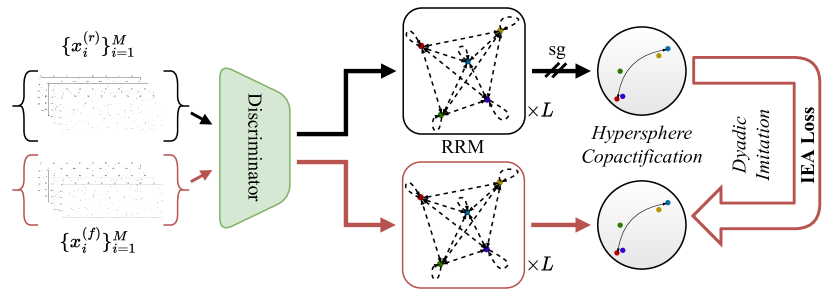
Figure 6: IEA-loss imposes a pair-wise fine-grained class-to-class imitation force for the generator. sg indicates that for the discriminator gradients are stopped and only the generator’s gradients will be updated.

Upon minimizing it for the generator (having the stop-gradient for the discriminator), we are putting a discriminator-supervised penalizing system over the intra-event awareness of the generator by encouraging it to look for more detailed dyadic connections among the images and be sensitive to even slight differences. Ultimately, we want to maximize the consensus of data points on two unit hyperspheres of real images and generated image embeddings.

4.5 Uniformity Loss

The other crucial loss function comes from contrastive representation learning. With the task of learning fine-grained class-to-class relations among the images, we also want to ensure the feature vectors have as much hyperspherical diversity as possible. Thus, by imposing a uniformity condition over the feature vectors on the unit hypersphere, they preserve as much information as possible since the uniform distribution carries a high entropy. This idea stems from the Thomson problem [86], where a static equilibrium with minimal potential energy is sought to distribute N electrons on the unit sphere in the evenest manner. To do that, we incorporate the uniformity metric [35], which is based on a Gaussian potential kernel,

$$\pazocal{L}_{\mathrm{uniform}}(x;s)=\log\mathbb{E}_{x_{i},x_{j}\sim p_{\mathrm{event}}}[\exp(s\|\mathbf{h}(x_{i})-\mathbf{h}(x_{j})\|_{2}^{2})].$$ (12)

Upon minimizing this loss for the discriminator, it tries to maintain a uniform distance among the samples that are not well-clustered and thus not similar. In other words, eventually, we want to reach a maximum geodesic separation incorporating the Riesz s-kernel [87] with $s=-2$ as a measure of geodesic similarity, to preserve maximal information over the Hypersphere. Therefore, asymptotically it corresponds to the uniform distribution on the hypersphere [88]. This loss is beneficial for capturing the exact distribution of the mean occupancy distribution and balancing the inter-class pulling force of the Relational Reasoning module. As a result, not only does it help generate more diverse and varied outputs, but it also can prevent issues such as mode collapse or overfitting.

4.6 Model Details and Hyperparameters

To capture the intra-event mutual information among the images using the RRM and approximate the concept of an event, we have to sample properly at each iteration. Hence, we utilize a one-sample per class sampler in data loading. Using this sampler, we ensure that in each event, we have 40 unique classes of images from all 40 sensors that belong to the same event in the Monte-Carlo simulation. All hyperparameters are chosen based on the model’s stability and performance upon the evaluation set. The learning rates for the Generator and Discriminator are $5\times 10^{-5}$ with one sample per class sampler. The Relational Reasoning Module of the Generator has two heads and one layer of non-spectrally normalized message propagation with an embedding dimension of 128 and ReLU non-linearity. The input to the generator’s RRM is embedded class tokens mixed with $4$ random degrees of freedom by a spectrally normalized linear layer.

For the Discriminator, the RRM has four heads with one layer of spectrally normalized message propagation with the embedding dimension $1024$ as the hypersphere dimension and ReLU non-linearity. All Generator and Discriminator modules use Orthogonal initialization [89]. For the IEA-loss in Equation 11, the coefficient $\lambda_{\mathrm{IEA}}=1.0$, defined in Algorithm 1 gives the best result. The most stable contribution of the Uniformity loss, defined in Equation 12 and Algorithm 1, is with $\lambda_{\mathrm{uniform}}=0.1$. For the backbone of both the discriminator and the generator, we use BigGAN-deep [48] with a non-local block at channel $32$ for the discriminator only. Since in GAN training, there is no meaningful way to define a minimal loss; our stopping point is the divergence of the Frechet Inception Score (FID) [44], which is significantly correlated with the quality of other metrics.

Algorithm 1 Intra-Event Aware GAN

1:generator and discriminator parameters $\theta_{G}$, $\theta_{D}$, Intra-Event-aware coefficient $\lambda_{\mathrm{IEA}}$, Uniformity coefficient $\lambda_{\mathrm{uniform}}$ and hyperparameter $s$, Adam hyperparameters $\alpha$, $\beta_{1}$, $\beta_{2}$, event size $M$, number of discriminator iteration steps per generator iteration $N_{D}$

2:

3:for number of training iterations do

4:     for $t=1,...,N_{D}$ do

5:         sample $\{z^{i}\}^{M}_{i=1}\sim p(z)$,

6:         $\{x^{i},y^{i}\}^{M}_{i=1}\sim p_{\mathrm{event}}(x,y)$, $\{r^{i}\}^{M}_{i=1}\sim p_{\mathrm{Rdof}}(z)$ $\triangleright$ Event Sampling.

7:         for $i=1,...,M$ do

8:              $\ell_{D_{\mathrm{hinge}}}^{(i)}\leftarrow\ell_{D_{\mathrm{hinge}}}(x^{(i)};G(z^{i},y^{i},r^{i}))$

9:         end for

10:         $\pazocal{L}_{D_{\mathrm{hinge}}}\leftarrow\frac{1}{M}\sum_{i=1}^{M}\ell_{D_{\mathrm{hinge}}}^{(i)}$

11:         $\pazocal{L}_{\mathrm{uniform}}\leftarrow\pazocal{L}_{\mathrm{uniform}}(x;s)$ $\triangleright$ The Uniformity Loss.

12:         $\pazocal{L}_{2C}^{\mathrm{real}}\leftarrow\frac{1}{M}\sum_{i=1}^{M}\ell_{2C}(x^{i},y^{i})$

13:         $\theta_{D}\leftarrow Adam(\pazocal{L}_{D_{\mathrm{hinge}}}+\lambda_{2C}\pazocal{L}_{2C}^{\mathrm{real}}+\lambda_{\mathrm{uniform}}\pazocal{L}_{\mathrm{uniform}},\alpha,\beta_{1},\beta_{2})$

14:     end for

15:     sample $\{z^{i}\}^{M}_{i=1}\sim p(z)$,

16:     sample $\{r^{i}\}^{M}_{i=1}\sim p_{\mathrm{Rdof}}(z)$ $\triangleright$ Event Sampling.

17:     for $i=1,...,M$ do

18:         $\ell_{G_{\mathrm{hinge}}}^{(i)}\leftarrow\ell_{G_{\mathrm{hinge}}}(G(z^{i},y^{i},r^{i}))$

19:     end for

20:     $\pazocal{L}_{G_{\mathrm{hinge}}}\leftarrow\frac{1}{M}\sum_{i=1}^{M}\ell_{G_{\mathrm{hinge}}}^{(i)}$

21:     $\pazocal{L}_{\mathrm{IEA}}\leftarrow\frac{1}{M}\sum_{i=1}^{M}\ell_{\mathrm{IEA}}(G(z^{i},y^{i},r^{i}),x^{i})$ $\triangleright$ The Intra-Event Aware Loss.

22:     $\pazocal{L}_{2C}^{\mathrm{fake}}\leftarrow\frac{1}{M}\sum_{i=1}^{M}\ell_{2C}(G(z^{i},y^{i},r^{i}),y^{i})$

23:     $\theta_{G}\leftarrow\mathrm{Adam}(\pazocal{L}_{G_{\mathrm{hinge}}}+\lambda_{2C}\pazocal{L}_{2C}^{\mathrm{fake}}+\lambda_{\mathrm{IEA}}\pazocal{L}_{\mathrm{IEA}},\alpha,\beta_{1},\beta_{2})$

24:end for

Declarations

Data availability

The data used in this study will be openly available (TBA).

Code availability

The code for this study is available at https://github.com/Hosein47/IEA-GAN.

Appendix A Ablation Studies and Things We Tried But Did Not Work

For the IEA-loss we tested several losses in order to achieve the best stability, shown in Figure 7. Some of them have their own merits and downsides. We explored the KL divergence, the L1 loss, the Huber loss [90], and the L2 loss. KL divergence was more stable to capture differences between the real and fake self-similarities and more robust to outliers.

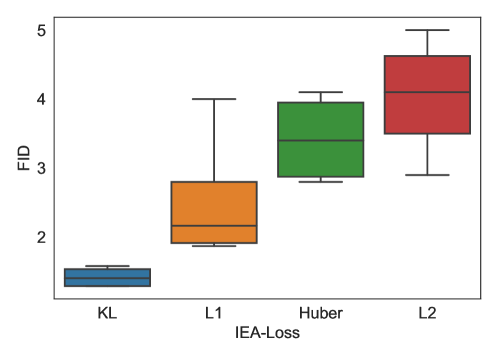
Figure 7: Comparison of the FID between different IEA-losses

We probed a range of coefficients for the IEA-loss and the Uniformity loss. For the KL divergence as the IEA-loss, we tried the values {0.1, 1, 5, 10} and selected $1$. For the L1 loss, as well as the IEA-loss the best $\lambda_{\mathrm{IEA}}$ value is $10$. For the Uniformity loss, we probed the values {0.01, 0.1, 0.5, 0.75, 1, 5, 10} and selected $0.1$. Moreover, IEA-GAN without the IEA-loss and Uniformity loss suffers from the lack of agreement maximization penalty for the generator and information maximization for the discriminator. Our study shows that having either of these losses without the other, causes training instability, divergence, and lower fidelity as shown in Table 3.

Table 3: FID comparison between IEA-GAN, IEA-GAN with RRM only, IEA-GAN with Uniformity loss only, and IEA-GAN with both IEA-loss, averaged across six random seeds.

	IEA-GAN	Only RRM	RRM with Uniformity	RRM with IEA-loss
FID	$\mathbf{1.50\pm 0.16}$	$2.74\pm 0.62$	$2.29\pm 0.14$	$3.42\pm 0.52$

For the hypersphere dimension, we probed the values {512, 768, 1024, 2048} and selected $1024$. For dimensions smaller than $512$ the discriminator fails to converge. We also changed the position of the hypersphere projection layer and put it before and after the Multi-head attention. The best position for the hypersphere projection is after the Multi-head attention and two layers of MLP. Moreover, for the hypersphere projection, we also tried an inverse Stereographic Projection $h:\mathbb{R}^{N}\rightarrow\mathbb{S}^{N}/\{p\}$ with p as a north pole on the n-sphere [91] instead of L2 compactification. This map is conformal thus it locally preserves angles between the data points. The results were more stable but the average FID was better with L2 compactification as shown in Table 4.

Table 4: FID comparison between two different Hypersphere projections for IEA-GAN’s discriminator, averaged across six random seeds.

	L2 compactification	Inverse Stereographic projection
FID	$\mathbf{1.50\pm 0.16}$	$2.01\pm 0.07$

Inside the RRM we tried a GeLU [92] non-linearity instead of ReLU and the result was in favor of the latter. We also put the layer normalization before and after the Multi-head Attention. The pre-norm version seems to be much more stable and adaptable to GAN training intricacies. Another observation related to RRM is the weight normalization of the linear layers. We observed that for the discriminator spectrally normalized MLPs show the best results. For the Generator, applying Spectral Normalization to the linear layers destabilizes the training. Our observation regarding the effect of RRM over the generator’s label embedding shows that without it, the RRM in the discriminator becomes also unstable and the training diverges very early.

For the random degrees of freedom (Rdof), first, we utilized the random vectors that are fed to the generator and applied the RRM on top of it. However, the FID did not reach values below $20$ and there was no correlation. Hence, we introduced separate random sampling for event generation for which we probed dimensions {2, 4, 8, 16, 32}. $4$ degrees of freedom was the most optimal choice. We observed that as the dimension of Rdof increases, the intra-event correlation fades away between the generated images. We also checked the Uniform distribution for event Rdof sampling, which did not lead to any stable result. Several ways to fuse the Rdof to the class embeddings were tested such as learnable neural network layer (matrix factorization), concatenating, summing, and having an MLP with non-linear part, but eventually chose a learnable neural network layer (matrix factorization) for the feature mixing layer.

We also looked at different combinations of learning rates for G and D. Using TTUR [44] regime results in a severe mode collapse. Thus, we used the same learning rates for both G and D. We swept through $\{1\times 10^{-5},2.5\times 10^{-5},5\times 10^{-5},7.5\times 10^{-5},1\times 10^{-4}\}$ and selected $5\times 10^{-5}$. For the backbone model, the shallow version of BigGAN-deep, BigGAN, lead to mode-collapse, therefore, we chose BigGAN-deep.

Appendix B Extended Figures and Tables

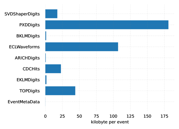
Figure 9: Data volume comparison of PXD data per event compared to other sub-detectors at Belle II

References

- de Oliveira et al. [2017] Luke de Oliveira, Michela Paganini, and Benjamin Nachman. Learning particle physics by example: location-aware generative adversarial networks for physics synthesis. Computing and Software for Big Science, 1(1):4, 2017.
- Paganini et al. [2018a] Michela Paganini, Luke de Oliveira, and Benjamin Nachman. Accelerating science with generative adversarial networks: an application to 3d particle showers in multilayer calorimeters. Physical review letters, 120(4):042003, 2018a.
- Paganini et al. [2018b] Michela Paganini, Luke de Oliveira, and Benjamin Nachman. Calogan: Simulating 3d high energy particle showers in multilayer electromagnetic calorimeters with generative adversarial networks. Physical Review D, 97(1):014021, 2018b.
- Vallecorsa [2018] Sofia Vallecorsa. Generative models for fast simulation. Journal of Physics: Conference Series, 1085:022005, September 2018. doi:10.1088/1742-6596/1085/2/022005.
- De Oliveira et al. [2018] Luke De Oliveira, Michela Paganini, and Benjamin Nachman. Controlling physical attributes in gan-accelerated simulation of electromagnetic calorimeters. In Journal of Physics: Conference Series, volume 1085, page 042017. IOP Publishing, 2018.
- Deja et al. [2020] Kamil Deja, Tomasz Trzciński, Łukasz Graczykowski, and ALICE Collaboration. Generative models for fast cluster simulations in the tpc for the alice experiment. In Information Technology, Systems Research, and Computational Physics 3, pages 267–280. Springer, 2020.
- Musella and Pandolfi [2018] Pasquale Musella and Francesco Pandolfi. Fast and accurate simulation of particle detectors using generative adversarial networks. Computing and Software for Big Science, 2(1):8, 2018.
- Chekalina et al. [2019] Viktoria Chekalina, Elena Orlova, Fedor Ratnikov, Dmitry Ulyanov, Andrey Ustyuzhanin, and Egor Zakharov. Generative models for fast calorimeter simulation: the lhcb case. In EPJ Web of Conferences, volume 214, page 02034. EDP Sciences, 2019.
- Di Sipio et al. [2019] Riccardo Di Sipio, Michele Faucci Giannelli, Sana Ketabchi Haghighat, and Serena Palazzo. Dijetgan: a generative-adversarial network approach for the simulation of qcd dijet events at the lhc. Journal of high energy physics, 2019(8), 2019.
- Erdmann et al. [2018] Martin Erdmann, Lukas Geiger, Jonas Glombitza, and David Schmidt. Generating and refining particle detector simulations using the wasserstein distance in adversarial networks. Computing and Software for Big Science, 2:1–9, 2018.
- Erdmann et al. [2019] Martin Erdmann, Jonas Glombitza, and Thorben Quast. Precise simulation of electromagnetic calorimeter showers using a wasserstein generative adversarial network. Computing and Software for Big Science, 3:1–13, 2019.
- Butter et al. [2019a] Anja Butter, Tilman Plehn, and Ramon Winterhalder. How to gan lhc events. SciPost Physics, 7(6):075, 2019a.
- Goodfellow et al. [2014] Ian J. Goodfellow, Jean Pouget-Abadie, Mehdi Mirza, Bing Xu, David Warde-Farley, Sherjil Ozair, Aaron Courville, and Yoshua Bengio. Generative Adversarial Networks, June 2014.
- Paganini et al. [2017] Michela Paganini, Luke de Oliveira, and Benjamin Nachman. CaloGAN: Simulating 3D High Energy Particle Showers in Multi-Layer Electromagnetic Calorimeters with Generative Adversarial Networks. Physical Review D, 97, December 2017. doi:10.1103/PhysRevD.97.014021.
- de Oliveira et al. [2018] Luke de Oliveira, Michela Paganini, and Benjamin Nachman. Controlling Physical Attributes in GAN-Accelerated Simulation of Electromagnetic Calorimeters. Journal of Physics: Conference Series, 1085:042017, September 2018. ISSN 1742-6596. doi:10.1088/1742-6596/1085/4/042017.
- KhattakTadahiro Nomura et al. [2022] Gul Rukh KhattakTadahiro Nomura, Sofia Vallecorsa, Federico Carminati, and Gul Muhammad Khan. Fast simulation of a high granularity calorimeter by generative adversarial networks. The European Physical Journal C, 82(4):386, April 2022. ISSN 1434-6052. doi:10.1140/epjc/s10052-022-10258-4.
- Alanazi et al. [2021a] Yasir Alanazi, Nobuo Sato, Pawel Ambrozewicz, Astrid Hiller-Blin, Wally Melnitchouk, Marco Battaglieri, Tianbo Liu, and Yaohang Li. A Survey of Machine Learning-Based Physics Event Generation. In Twenty-Ninth International Joint Conference on Artificial Intelligence, volume 5, pages 4286–4293, August 2021a. doi:10.24963/ijcai.2021/588.
- Butter et al. [2019b] Anja Butter, Tilman Plehn, and Ramon Winterhalder. How to GAN LHC events. SciPost Physics, 7(6):075, December 2019b. ISSN 2542-4653. doi:10.21468/SciPostPhys.7.6.075.
- Otten et al. [2021] Sydney Otten, Sascha Caron, Wieske de Swart, Melissa van Beekveld, Luc Hendriks, Caspar van Leeuwen, Damian Podareanu, Roberto Ruiz de Austri, and Rob Verheyen. Event generation and statistical sampling for physics with deep generative models and a density information buffer. Nature Communications, 12(1):2985, May 2021. ISSN 2041-1723. doi:10.1038/s41467-021-22616-z.
- Hashemi et al. [2021] Hosein Hashemi, Nikolai Hartmann, Thomas Kuhr, Martin Ritter, and Matej Srebre. Pixel Detector Background Generation using Generative Adversarial Networks at Belle II. EPJ Web of Conferences, 251:03031, January 2021. doi:10.1051/epjconf/202125103031.
- Srebre et al. [2020] Matej Srebre, Pascal Schmolz, Hosein Hashemi, Martin Ritter, and Thomas Kuhr. Generation of Belle II Pixel Detector Background Data with a GAN. EPJ Web Conf., 245:02010, 2020. doi:10.1051/epjconf/202024502010.
- Arjovsky et al. [2017] Martin Arjovsky, Soumith Chintala, and Léon Bottou. Wasserstein generative adversarial networks. In International conference on machine learning, pages 214–223. PMLR, 2017.
- Gulrajani et al. [2017] Ishaan Gulrajani, Faruk Ahmed, Martin Arjovsky, Vincent Dumoulin, and Aaron Courville. Improved training of wasserstein GANs. In Proceedings of the 31st International Conference on Neural Information Processing Systems, NIPS’17, pages 5769–5779, Red Hook, NY, USA, December 2017. Curran Associates Inc. ISBN 978-1-5108-6096-4.
- Buhmann et al. [2021] Erik Buhmann, Sascha Diefenbacher, Engin Eren, Frank Gaede, Gregor Kasieczka, Anatolii Korol, and Katja Krüger. Getting high: high fidelity simulation of high granularity calorimeters with high speed. Computing and Software for Big Science, 5(1):13, 2021.
- Krause and Shih [2021] Claudius Krause and David Shih. Caloflow ii: Even faster and still accurate generation of calorimeter showers with normalizing flows. arXiv preprint arXiv:2110.11377, 2021.
- Rezende and Mohamed [2015] Danilo Rezende and Shakir Mohamed. Variational inference with normalizing flows. In International conference on machine learning, pages 1530–1538. PMLR, 2015.
- Deselaers and Ferrari [2011] Thomas Deselaers and Vittorio Ferrari. Visual and semantic similarity in imagenet. In CVPR 2011, pages 1777–1784. IEEE, 2011.
- Wei et al. [2021] Xiu-Shen Wei, Yi-Zhe Song, Oisin Aodha, Jianxin Wu, Yuxin Peng, Jinhui Tang, Jian Yang, and Serge Belongie. Fine-Grained Image Analysis with Deep Learning: A Survey. IEEE Transactions on Pattern Analysis and Machine Intelligence, PP:1–1, November 2021. doi:10.1109/TPAMI.2021.3126648.
- Zhang et al. [2019] Han Zhang, Ian Goodfellow, Dimitris Metaxas, and Augustus Odena. Self-Attention Generative Adversarial Networks. In Proceedings of the 36th International Conference on Machine Learning, volume 97 of Proceedings of Machine Learning Research, pages 7354–7363, CA, USA, May 2019. PMLR.
- Miyato and Koyama [2018] Takeru Miyato and Masanori Koyama. cGANs with Projection Discriminator, August 2018.
- Kang and Park [2020] Minguk Kang and Jaesik Park. ContraGAN: Contrastive Learning for Conditional Image Generation. In Advances in Neural Information Processing Systems, volume 33, pages 21357–21369, Virtual, 2020. Curran Associates, Inc.
- Kang et al. [2021] Minguk Kang, Woohyeon Shim, Minsu Cho, and Jaesik Park. Rebooting ACGAN: Auxiliary Classifier GANs with Stable Training. In Advances in Neural Information Processing Systems, volume 34, pages 23505–23518, Virtual, 2021. Curran Associates, Inc.
- Rangwani et al. [2021] Harsh Rangwani, Konda Reddy Mopuri, and R Venkatesh Babu. Class balancing gan with a classifier in the loop. In Uncertainty in Artificial Intelligence, pages 1618–1627. PMLR, 2021.
- Cao [2015] Longbing Cao. Coupling learning of complex interactions. Information Processing & Management, 51(2):167–186, March 2015. ISSN 0306-4573. doi:10.1016/j.ipm.2014.08.007.
- Wang and Isola [2020] Tongzhou Wang and Phillip Isola. Understanding Contrastive Representation Learning through Alignment and Uniformity on the Hypersphere. In Proceedings of the 37th International Conference on Machine Learning, volume 119 of Proceedings of Machine Learning Research, pages 9929–9939, Vienna, Austria, November 2020. PMLR.
- Mueller [2014] F. Mueller. Some aspects of the Pixel Vertex Detector (PXD) at Belle II. Journal of Instrumentation, 9(10):C10007–C10007, October 2014. ISSN 1748-0221. doi:10.1088/1748-0221/9/10/C10007.
- Abe et al. [2010] Tetsuo Abe, I Adachi, K Adamczyk, S Ahn, H Aihara, K Akai, M Aloi, L Andricek, K Aoki, Y Arai, et al. Belle ii technical design report. arXiv preprint arXiv:1011.0352, 2010.
- Nash [1951] John Nash. Non-Cooperative Games. Annals of Mathematics, 54(2):286–295, 1951. ISSN 0003-486X. doi:10.2307/1969529.
- Battaglia et al. [2018] Peter W Battaglia, Jessica B Hamrick, Victor Bapst, Alvaro Sanchez-Gonzalez, Vinicius Zambaldi, Mateusz Malinowski, Andrea Tacchetti, David Raposo, Adam Santoro, Ryan Faulkner, et al. Relational inductive biases, deep learning, and graph networks. arXiv preprint arXiv:1806.01261, 2018.
- Sharifzadeh et al. [2021] Sahand Sharifzadeh, Sina Moayed Baharlou, and Volker Tresp. Classification by Attention: Scene Graph Classification with Prior Knowledge. Proceedings of the AAAI Conference on Artificial Intelligence, 35(6):5025–5033, May 2021. ISSN 2374-3468. doi:10.1609/aaai.v35i6.16636.
- Locatello et al. [2020] Francesco Locatello, Dirk Weissenborn, Thomas Unterthiner, Aravindh Mahendran, Georg Heigold, Jakob Uszkoreit, Alexey Dosovitskiy, and Thomas Kipf. Object-centric learning with slot attention. Advances in Neural Information Processing Systems, 33:11525–11538, 2020.
- Devlin et al. [2018] Jacob Devlin, Ming-Wei Chang, Kenton Lee, and Kristina Toutanova. Bert: Pre-training of deep bidirectional transformers for language understanding. arXiv preprint arXiv:1810.04805, 2018.
- Zhang and Yang [2018] Dongxu Zhang and Zhichao Yang. Word Embedding Perturbation for Sentence Classification, April 2018.
- Heusel et al. [2017] Martin Heusel, Hubert Ramsauer, Thomas Unterthiner, Bernhard Nessler, and Sepp Hochreiter. GANs trained by a two time-scale update rule converge to a local nash equilibrium. In Proceedings of the 31st International Conference on Neural Information Processing Systems, NIPS’17, pages 6629–6640, Red Hook, NY, USA, December 2017. Curran Associates Inc. ISBN 978-1-5108-6096-4.
- Parmar et al. [2022] Gaurav Parmar, Richard Zhang, and Jun-Yan Zhu. On Aliased Resizing and Surprising Subtleties in GAN Evaluation. In Proceedings of the IEEE/CVF Conference on Computer Vision and Pattern Recognition, pages 11410–11420, 2022.
- Szegedy et al. [2016] Christian Szegedy, Vincent Vanhoucke, Sergey Ioffe, Jon Shlens, and Zbigniew Wojna. Rethinking the Inception Architecture for Computer Vision. In 2016 IEEE Conference on Computer Vision and Pattern Recognition (CVPR), pages 2818–2826, June 2016. doi:10.1109/CVPR.2016.308.
- Agostinelli et al. [2003] Sea Agostinelli, John Allison, K al Amako, John Apostolakis, H Araujo, Pedro Arce, Makoto Asai, D Axen, Swagato Banerjee, GJNI Barrand, et al. Geant4—a simulation toolkit. Nuclear instruments and methods in physics research section A: Accelerators, Spectrometers, Detectors and Associated Equipment, 506(3):250–303, 2003.
- Brock et al. [2019] Andrew Brock, Jeff Donahue, and Karen Simonyan. Large scale GAN training for high fidelity natural image synthesis. In International Conference on Learning Representations, 2019. URL https://openreview.net/forum?id=B1xsqj09Fm.
- Braun et al. [2018] Nils Braun, T. Kuhr, M. Ritter, C. Pulvermacher, and Thomas Hauth. The Belle II Core Software. Computing and Software for Big Science, 3, November 2018. doi:10.1007/s41781-018-0017-9.
- Kou et al. [2020] E Kou et al. The Belle II Physics Book. Progress of Theoretical and Experimental Physics, 2020(2):029201, February 2020. ISSN 2050-3911. doi:10.1093/ptep/ptaa008.
- Liu et al. [2019] Yinhan Liu, Myle Ott, Naman Goyal, Jingfei Du, Mandar Joshi, Danqi Chen, Omer Levy, Mike Lewis, Luke Zettlemoyer, and Veselin Stoyanov. Roberta: A robustly optimized bert pretraining approach. arXiv preprint arXiv:1907.11692, 2019.
- Yang et al. [2019] Zhilin Yang, Zihang Dai, Yiming Yang, Jaime Carbonell, Russ R Salakhutdinov, and Quoc V Le. Xlnet: Generalized autoregressive pretraining for language understanding. Advances in neural information processing systems, 32, 2019.
- Hariri et al. [2021] Ali Hariri, Darya Dyachkova, and Sergei Gleyzer. Graph Generative Models for Fast Detector Simulations in High Energy Physics, August 2021.
- Verheyen [2022] Rob Verheyen. Event Generation and Density Estimation with Surjective Normalizing Flows. SciPost Physics, 13(3):047, September 2022. ISSN 2542-4653. doi:10.21468/SciPostPhys.13.3.047.
- Alanazi et al. [2021b] Yasir Alanazi, Nobuo Sato, Pawel Ambrozewicz, Astrid N Hiller Blin, Wally Melnitchouk, Marco Battaglieri, Tianbo Liu, and Yaohang Li. A survey of machine learning-based physics event generation. arXiv preprint arXiv:2106.00643, 2021b.
- Butter et al. [2022] Anja Butter, Tilman Plehn, Steffen Schumann, Simon Badger, Sascha Caron, Kyle Cranmer, Francesco Armando Di Bello, Etienne Dreyer, Stefano Forte, Sanmay Ganguly, et al. Machine learning and lhc event generation. arXiv preprint arXiv:2203.07460, 2022.
- Evans and Bryant [2008] Lyndon Evans and Philip Bryant. LHC Machine. Journal of Instrumentation, 3(08):S08001–S08001, August 2008. ISSN 1748-0221. doi:10.1088/1748-0221/3/08/S08001.
- Apollinari et al. [2017] Giorgio Apollinari, I Béjar Alonso, O Brüning, P Fessia, M Lamont, L Rossi, and L Tavian. High-luminosity large hadron collider (hl-lhc). technical design report v. 0.1. Technical report, Fermi National Accelerator Lab.(FNAL), Batavia, IL (United States), 2017.
- Huang et al. [2016] Po-Ssu Huang, Scott E Boyken, and David Baker. The coming of age of de novo protein design. Nature, 537(7620):320–327, 2016.
- Liu et al. [2021] Qiao Liu, Jiaze Xu, Rui Jiang, and Wing Hung Wong. Density estimation using deep generative neural networks. Proceedings of the National Academy of Sciences, 118(15):e2101344118, 2021.
- Repecka et al. [2021] Donatas Repecka, Vykintas Jauniskis, Laurynas Karpus, Elzbieta Rembeza, Irmantas Rokaitis, Jan Zrimec, Simona Poviloniene, Audrius Laurynenas, Sandra Viknander, Wissam Abuajwa, et al. Expanding functional protein sequence spaces using generative adversarial networks. Nature Machine Intelligence, 3(4):324–333, 2021.
- Anand and Huang [2018] Namrata Anand and Possu Huang. Generative modeling for protein structures. Advances in neural information processing systems, 31, 2018.
- Strokach and Kim [2022] Alexey Strokach and Philip M Kim. Deep generative modeling for protein design. Current opinion in structural biology, 72:226–236, 2022.
- Kim et al. [2017] DY Kim, M Ritter, T Bilka, A Bobrov, G Casarosa, K Chilikin, T Ferber, R Godang, I Jaegle, J Kandra, et al. The simulation library of the belle ii software system. In Journal of Physics: Conference Series, volume 898, page 042043. IOP Publishing, 2017.
- Kuhr [2011] Thomas Kuhr. Computing at Belle II. Journal of Physics: Conference Series, 331(7):072021, December 2011. ISSN 1742-6596. doi:10.1088/1742-6596/331/7/072021.
- Mirza and Osindero [2014] Mehdi Mirza and Simon Osindero. Conditional generative adversarial nets. arXiv preprint arXiv:1411.1784, 2014.
- Lim and Ye [2017] Jae Hyun Lim and Jong Chul Ye. Geometric GAN, May 2017.
- Odena et al. [2017] Augustus Odena, Christopher Olah, and Jonathon Shlens. Conditional image synthesis with auxiliary classifier GANs. In Proceedings of the 34th International Conference on Machine Learning - Volume 70, ICML’17, pages 2642–2651, Sydney, NSW, Australia, August 2017. JMLR.org.
- Chen et al. [2020] Ting Chen, Simon Kornblith, Mohammad Norouzi, and Geoffrey Hinton. A simple framework for contrastive learning of visual representations. In Proceedings of the 37th International Conference on Machine Learning, ICML’20, pages 1597–1607, Virtual, July 2020. JMLR.org.
- Vaswani et al. [2017] Ashish Vaswani, Noam Shazeer, Niki Parmar, Jakob Uszkoreit, Llion Jones, Aidan N. Gomez, Łukasz Kaiser, and Illia Polosukhin. Attention is all you need. In Proceedings of the 31st International Conference on Neural Information Processing Systems, NIPS’17, pages 6000–6010, Red Hook, NY, USA, December 2017. Curran Associates Inc. ISBN 978-1-5108-6096-4.
- Hudson and Zitnick [2021] Drew A. Hudson and Larry Zitnick. Generative Adversarial Transformers. In Proceedings of the 38th International Conference on Machine Learning, pages 4487–4499, Virtual, July 2021. PMLR.
- Jiang et al. [2021] Yifan Jiang, Shiyu Chang, and Zhangyang Wang. TransGAN: Two Pure Transformers Can Make One Strong GAN, and That Can Scale Up. In Advances in Neural Information Processing Systems, volume 34, pages 14745–14758, Virtual, 2021. Curran Associates, Inc.
- Dosovitskiy et al. [2022] Alexey Dosovitskiy, Lucas Beyer, Alexander Kolesnikov, Dirk Weissenborn, Xiaohua Zhai, Thomas Unterthiner, Mostafa Dehghani, Matthias Minderer, Georg Heigold, Sylvain Gelly, Jakob Uszkoreit, and Neil Houlsby. An Image is Worth 16x16 Words: Transformers for Image Recognition at Scale. In International Conference on Learning Representations, March 2022.
- Liu et al. [2020] Liyuan Liu, Xiaodong Liu, Jianfeng Gao, Weizhu Chen, and Jiawei Han. Understanding the Difficulty of Training Transformers. January 2020. doi:10.18653/v1/2020.emnlp-main.463.
- Clark et al. [2019] Kevin Clark, Urvashi Khandelwal, Omer Levy, and Christopher Manning. What Does BERT Look at? An Analysis of BERT’s Attention. January 2019. doi:10.18653/v1/W19-4828.
- Yun et al. [2020] Chulhee Yun, Srinadh Bhojanapalli, Ankit Singh Rawat, Sashank J. Reddi, and Sanjiv Kumar. Are Transformers universal approximators of sequence-to-sequence functions?, February 2020.
- Guttenberg et al. [2016] Nicholas Guttenberg, Nathaniel Virgo, Olaf Witkowski, Hidetoshi Aoki, and Ryota Kanai. Permutation-equivariant neural networks applied to dynamics prediction. arXiv preprint arXiv:1612.04530, 2016.
- Ravanbakhsh et al. [2017] Siamak Ravanbakhsh, Jeff Schneider, and Barnabas Poczos. Equivariance through parameter-sharing. In International conference on machine learning, pages 2892–2901. PMLR, 2017.
- Zaheer et al. [2017] Manzil Zaheer, Satwik Kottur, Siamak Ravanbhakhsh, Barnabás Póczos, Ruslan Salakhutdinov, and Alexander J Smola. Deep Sets. In Proceedings of the 31st International Conference on Neural Information Processing Systems, NIPS’17, pages 3394–3404, Red Hook, NY, USA, December 2017. Curran Associates Inc. ISBN 978-1-5108-6096-4.
- Ba et al. [2016] Jimmy Lei Ba, Jamie Ryan Kiros, and Geoffrey E. Hinton. Layer Normalization, July 2016.
- Miyato et al. [2022] Takeru Miyato, Toshiki Kataoka, Masanori Koyama, and Yuichi Yoshida. Spectral Normalization for Generative Adversarial Networks. In International Conference on Learning Representations, March 2022.
- Wang et al. [2017] Feng Wang, Xiang Xiang, Jian Cheng, and Alan Yuille. NormFace: L2 Hypersphere Embedding for Face Verification. October 2017. doi:10.1145/3123266.3123359.
- Gorban and Tyukin [2017] Alexander Gorban and Ivan Tyukin. Stochastic Separation Theorems. Neural Networks, 94:255–259, November 2017. doi:10.1016/j.neunet.2017.07.014.
- Weng [2019] Lilian Weng. Self-supervised representation learning. lilianweng.github.io, 2019. URL https://lilianweng.github.io/posts/2019-11-10-self-supervised/.
- Kullback and Leibler [1951] S. Kullback and R. A. Leibler. On Information and Sufficiency. The Annals of Mathematical Statistics, 22(1):79–86, March 1951. ISSN 0003-4851, 2168-8990. doi:10.1214/aoms/1177729694.
- Thomson [1904] J.J. Thomson. XXIV. On the structure of the atom: An investigation of the stability and periods of oscillation of a number of corpuscles arranged at equal intervals around the circumference of a circle; with application of the results to the theory of atomic structure. The London, Edinburgh, and Dublin Philosophical Magazine and Journal of Science, 7(39):237–265, March 1904. ISSN 1941-5982. doi:10.1080/14786440409463107.
- Liu et al. [2018] Weiyang Liu, Rongmei Lin, Zhen Liu, Lixin Liu, Zhiding Yu, Bo Dai, and Le Song. Learning towards minimum hyperspherical energy. Advances in neural information processing systems, 31, 2018.
- Kuijlaars and Saff [1998] A. Kuijlaars and E. Saff. Asymptotics for minimal discrete energy on the sphere. Transactions of the American Mathematical Society, 350(2):523–538, 1998. ISSN 0002-9947, 1088-6850. doi:10.1090/S0002-9947-98-02119-9.
- Saxe et al. [2014] Andrew M. Saxe, James L. McClelland, and Surya Ganguli. Exact solutions to the nonlinear dynamics of learning in deep linear neural networks, February 2014.
- Huber [1992] Peter J Huber. Robust estimation of a location parameter. In Breakthroughs in statistics, pages 492–518. Springer, 1992.
- Eybpoosh et al. [2022] Kajal Eybpoosh, Mansoor Rezghi, and Abbas Heydari. Applying inverse stereographic projection to manifold learning and clustering. Applied Intelligence, 52(4):4443–4457, March 2022. ISSN 0924-669X. doi:10.1007/s10489-021-02513-0.
- Hendrycks and Gimpel [2020] Dan Hendrycks and Kevin Gimpel. Gaussian Error Linear Units (GELUs), July 2020.