Helicoidal minimal surfaces in the 3-sphere:
An approach via spherical curves

Abstract.

We prove an existence and uniqueness theorem about spherical helicoidal (in particular, rotational) surfaces with prescribed mean or Gaussian curvature in terms of a continuous function depending on the distance to its axis. As an application in the case of vanishing mean curvature, it is shown that the well-known conjugation between the belicoid and the catenoid in Euclidean three-space extends naturally to the 3-sphere to their spherical versions and determine in a quite explicit way their associated surfaces in the sense of Lawson. As a key tool, we use the notion of spherical angular momentum of the spherical curves that play the role of profile curves of the minimal helicoidal surfaces in the 3-sphere.

1. Introduction

The study of minimal surfaces is one the most important research fields in differential geometry. Minimal surfaces locally minimize area, that is, they are critical points of the area functional and are characterized as surfaces whose mean curvature vanishes everywhere. It is particularly interesting to study minimal surfaces in $3$-manifolds of constant curvature, such as the Euclidean space $\mathbb{R}^{3}$, the hyperbolic space $\mathbb{H}^{3}$, and the sphere $\mathbb{S}^{3}$.

Minimal surfaces in $\mathbb{R}^{3}$ have been an intensively studied classic topic (see e.g. [MP12] and references therein): Euler discovered in 1741 that a catenary rotating around a suitable axis provides a surface, called the catenoid, which minimizes area among surfaces of revolution after prescribing boundary values. The catenoid is the only minimal surface of revolution, up to the plane (Bonnet, 1860). The helicoid was first proved to be minimal by Meusnier in 1776. Catalan showed in 1842 that the helicoid, together with the plane, are the only ruled minimal surfaces.

It is pointed out for minimal surfaces in Euclidean $3$-space the beautiful property of existence of a $1$-parameter family of minimal isometric surfaces (the so called associated surfaces) connecting the catenoid and the helicoid, which are said to be conjugate each other. The associated surfaces are precisely the minimal helicoidal surfaces studied by Scherk in 1834. Viewing this family through their Weierstrass representation formula, one may see that they vary depending on their Bonnet angle and represent, in some way, a complex rotation of the classical (right) helicoid. They are also Björling surfaces associated to a circular helix. For the catenoid, the helix becomes a circle and in the case of the helicoid, it becomes the axis (cf. [F93]).

The first aim of this paper is to analyze in depth the spherical version of the possible existence of an isometric family of minimal surfaces connecting the catenoid to the helicoid. To do so, we will first have to determine which surfaces play the role of helicoids and catenoids in the 3-sphere.

Differently as happen in $\mathbb{R}^{3}$, interesting examples of closed minimal surfaces exist in $\mathbb{S}^{3}=\{(x_{1},x_{2},x_{3},x_{4})\in\mathbb{R}^{4}:x_{1}^{2}+x_{2}^{2}+x_{3}^{2}+x_{4}^{2}=1\}$, which are characterized by remarkable uniqueness theorems (see e.g. [Br13b] and references therein): The simplest is the totally geodesic equatorial 2-sphere, whose principal curvatures are both equal to zero. Using Hopf differential arguments, Almgren proved in 1966 that it is the only immersed minimal surface of genus $0$ in $\mathbb{S}^{3}$. Another important example of a closed minimal surface in $\mathbb{S}^{3}$ is the Clifford torus, given by $x_{1}^{2}+x_{2}^{2}=x_{3}^{2}+x_{4}^{2}=1/2$, whose principal curvatures are $1$ and $-1$. Brendle proved in [Br13a] that it is the only embedded minimal surface in $\mathbb{S}^{3}$ of genus $1$, thereby giving an affirmative answer to Lawson’s Conjecture (cf. [La70]). Brendle technique was pioneered by Huisken and involves an application of the maximum principle to a two-point function. In addition, we remark the following local rigidity result ([La69]) concerning these two main examples: the equatorial $2$-sphere and the Clifford torus are the only minimal surfaces of constant Gauss curvature ($1$ and $0$, respectively) in $\mathbb{S}^{3}$. Moreover, these are the only minimal surfaces of cohomogeneity zero on $\mathbb{S}^{3}$.

In 1970 Lawson constructed in [La70, Theorem 3] an explicit infinite family $\tau_{m,k}$, with $m,k$ positive integers such that $(m,k)=1$, of immersed minimal tori in $\mathbb{S}^{3}$ which fail to be embedded. They can be explicitly described by the doubly periodic immersions $\Psi_{h}:\mathbb{R}^{2}\rightarrow\mathbb{S}^{3}$ given by

$$\Psi_{h}(s,t)=\left(\cos s\cos ht,\cos s\sin ht,\sin s\cos t,\sin s\sin t\right)$$

by taking $h=m/k$. We recall (see [La70, Proposition 7.2]) that $\Psi_{h}$ are the only geodesically ruled minimal surfaces in $\mathbb{S}^{3}$ and so it is natural that they are referred to as Lawson spherical helicoids.

To find the spherical version of the catenoids, it is therefore natural to concentrate on the rotational minimal surfaces of $\mathbb{S}^{3}$. Do Carmo and Dajczer, in their classical paper [dCD83] on rotation hypersurfaces in spaces of constant curvature, coin the term ”catenoids” for those minimal rotational surfaces both in the hyperbolic space $\mathbb{H}^{3}$ (where the catenoids are of three different types) and in the sphere $\mathbb{S}^{3}$, similar to what happens in Euclidean space $\mathbb{R}^{3}$ where they recover the differential equation to be satisfied by the catenary as generatrix curve of the corresponding surface of revolution. The hyperbolic case is studied in depth in [dCD83], while for the spherical case the expected analogous results are discussed in several remarks, without going into too much detail. For example, in [dCD83, Remark (3.34)] it is commented that a conjugate correspondence can be established between the catenoids in $\mathbb{S}^{3}$ and the Lawson spherical helicoids. And in [dCD83, Remark (3.35)] it is stated that it is possible to determine explicitly the associated family of the catenoids in $\mathbb{S}^{3}$ but the authors will not go into that in the paper.

On the other hand, we must mention that $SO(2)$-invariant minimal surfaces in $\mathbb{S}^{3}$ were also determined in a slightly different and quite implicit way in [Ot70]. In fact, Otsuki studied in [Ot70] minimal hypersurfaces of $\mathbb{S}^{n+1}$ with two distinct principal curvatures. When restricted to the case $n=2$, the constructed compact surfaces are indeed tori, and they were named Otsuki tori in [Pn13], where they were re-defined as a part of a general construction by Hsiang and Lawson of minimal submanifolds of low cohomogeneity proposed in [HL71]. Most interestingly, Penskoi [Pn13] showed that the Otsuki tori provide an extremal metric for the invariant spectral functional. We highlight the rather more explicit description of them in [HS12]. Lawson himself remarked in [La70] that the tori $\tau_{m,k}$ are not the ones known to T. Otsuki [Ot70] or E. Calabi [Ca67] because the self-congruence groups are inequivalent.

Moreover, an analytical description of the minimal rotational surfaces of $\mathbb{S}^{3}$ is given in [Ri89, Theorem A] in the spirit of [dCD83], determining a one parameter family of compact minimal rotational surfaces.

But we must also pay attention to a more recent family of immersed minimal tori in $\mathbb{S}^{3}$ which are rotationally symmetric (see [Br13b, Theorem 1.4], pointed out by Robert Kusner, according to the author). These surfaces are not embedded, but they turn out to be immersed in the sense of Alexandrov, providing a large family of Alexandrov immersed minimal surfaces in $\mathbb{S}^{3}$. We will call them Brendle-Kusner tori. Brendle extended his argument used to prove Lawson’s Conjecture showing in [Br13c] that any minimal torus which is immersed in the sense of Alexandrov must be rotationally symmetric.

Therefore, our second goal in this article will be to fully justify which surfaces of $\mathbb{S}^{3}$ and why deserve the appellation of spherical catenoids, by clearly and concisely unifying the different examples of rotational minimal surfaces in $\mathbb{S}^{3}$ that one can find in the literature, which will come to be the conjugate surfaces to the geodesically ruled minimal surfaces in $\mathbb{S}^{3}$, that is, the Lawson spherical helicoids. In other words, we will show in detail that the well-known conjugation between the belicoid and the catenoid in Euclidean three-space extends to the spherical case. In fact, we will determine explicitly their associated family.

In order to achieve this objective, we deal in Section 2 with helicoidal surfaces in the unit $3$-sphere $\mathbb{S}^{3}$, i.e. surfaces invariant under the action of the helicoidal $1$-parameter group of isometries given by the composition of a translation and a rotation in $\mathbb{S}^{3}$. This class includes the rotational ones. As a key tool, we introduce in Section 3 the notion of spherical angular momentum of a spherical curve. It is a smooth function associated to any spherical curve, which completely determines it (up to a family of distinguished isometries) in relation with its relative position with respect to a fixed geodesic (see Theorem 3.1). We compute it for great and small circles and for the classical spherical catenaries studied by Bobillier and Gudermann in nineteenth century. Then we introduce a one-parameter family of spherical catenoids in Definition 3.6 just as the rotational surfaces generated by the above mentioned classical spherical catenaries. They turn to be the minimal rotational surfaces in $\mathbb{S}^{3}$ considered in [dCD83] and [Ri89].

The spherical angular momentum of the profile spherical curve of a helicoidal surface will play a fundamental role since it determines the geometry of the helicoidal surface, joint to its pitch, according to Corollary 4.1. So we are able to prove an existence and uniqueness result (Theorem 4.4) showing that if we prescribe the mean or the Gaussian curvature of a spherical helicoidal (in particular, rotational) surface in terms of a continuous function depending on the distance to its axis, once the pitch is set we get a one parameter family of helicoidal surfaces with this prescribed mean or Gaussian curvature determined by the spherical angular momenta of their profile curves.

As a first application, in Theorem 5.2 we perform in an easy direct way the local classification of the minimal rotational surfaces of $\mathbb{S}^{3}$ in terms of the spherical catenoids, together with the totally geodesic sphere and the Clifford torus that appear as limiting cases. Moreover, in Theorem 5.2, we also identify both Otsuki and Brendle-Kusner tori with the compact spherical catenoids, resulting the only Alexandrov immersed minimal tori in $\mathbb{S}^{3}$.

In Theorem 5.4, we make a first approach to the assertion of [dCD83, Remark (3.34)] by showing explicitly that each spherical catenoid is locally isometric to two, and only two, spherical Lawson helicoids and, as expected, the Clifford torus seems to appear as a self-conjugate surface (see Remarks 5.5 and 5.8).

Finally, on the basis of our rather explicit description of all the minimal helicoidal surfaces in $\mathbb{S}^{3}$ in terms of their spherical angular momenta, we prove in Theorem 5.6 that they are the associated surfaces (in the sense of [La70]) to the spherical catenoids and confirm the conjugation between spherical catenoids and Lawson spherical helicoids suggested in Theorem 5.4. In this way, we carry out the statement of [dCD83, Remark (3.35)] in detail.

Acknowledgments. The authors are very grateful to Marcos Dajczer, José Miguel Manzano, Pablo Mira, Miguel Sánchez, Francisco Torralbo and Francisco Urbano for helpful and fruitful discussions.

2. Helicoidal and rotational surfaces in the 3-sphere

Throughout this paper we will identify the 3-sphere $\mathbb{S}^{3}$ with the unit sphere in $\mathbb{R}^{4}$; that is,

$$\mathbb{S}^{3}=\{(x_{1},x_{2},x_{3},x_{4})\in\mathbb{R}^{4}:x_{1}^{2}+x_{2}^{2}+x_{3}^{2}+x_{4}^{2}=1\}.$$

A helicoidal surface in $\mathbb{S}^{3}$ is a surface invariant under the action of the helicoidal 1-parameter group of isometries given by the composition of a translation and a rotation in $\mathbb{S}^{3}$. Concretely, for any $a\in\mathbb{R}$, let $\psi_{a}(t)$ be the translations along the great circle $c_{0}=\{(x_{1},x_{2},0,0)\in\mathbb{S}^{3}\}$ given by

$$\psi_{a}(t)=\left(\begin{array}[]{cccc}\cos at&-\sin at&0&0\\ \sin at&\cos at&0&0\\ 0&0&1&0\\ 0&0&0&1\end{array}\right),$$

and for any $b\neq 0$, let $\phi_{b}(t)$ be the rotations around $c_{0}$ given by

$$\phi_{b}(t)=\left(\begin{array}[]{cccc}1&0&0&0\\ 0&1&0&0\\ 0&0&\cos bt&-\sin bt\\ 0&0&\sin bt&\cos bt\end{array}\right).$$

We remark that the group $\phi_{b}(t)$ fixes the great circle $c_{0}$ and the orbits are circles centred on $c_{0}$.

Hence, a helicoidal surface (along the great circle $c_{0}$) is invariant under $\psi_{a}(t)\circ\phi_{b}(t)$, for fixed translation velocity $a\in\mathbb{R}$ and rotation velocity $b\neq 0$, and can be locally parametrized by

(2.1) $$X_{b}^{a}(\xi)(s,t)=\psi_{a}(t)(\phi_{b}(t)\,\xi(s)),$$

where $\xi:I\subseteq\mathbb{R}\rightarrow\mathbb{S}^{2}_{+}$ is a regular curve in the half totally geodesic sphere $\mathbb{S}^{2}_{+}=\{(x_{1},x_{2},x_{3},0)\in\mathbb{S}^{3}\,:x_{3}>0\}$ of $\mathbb{S}^{3}$, called the profile curve (cf. [MdS19]).

Remark 2.1.

Up to the change of parameter $\tilde{t}=b\,t$ we could consider simply $b=1$. In other words, for a helicoidal surface $X^{a}_{b}(\xi)$ the essential parameter is the ratio $h=a/b\in\mathbb{R}$ called the pitch. For this reason, we will simply denote $X^{h}=X^{a}_{b}$ when we choose $b=1$ and so $a=h$. In addition, there is no restriction if we consider $a\geq 0$, $b>0$; that is, $h\geq 0$.

If $h=0$, $\psi_{0}$ is the identity and then $X^{0}(\xi)(s,t)=\phi_{1}(t)\,\xi(s)$ is a rotational surface with axis $c_{0}$ and the profile curve $\xi$ is its generating curve.

If $h=1$, the isometries $\psi_{1}(t)\circ\phi_{1}(t)$ are usually known as Clifford translations. In this case, the orbits are all great circles, which are equidistant from each other, and coincide with the fibers of the Hopf fibration $\pi\colon\mathbb{S}^{3}\rightarrow\mathbb{S}^{2}$.

If we put $\xi(s)=(x(s),y(s),z(s),0)$, with $x(s)^{2}+y(s)^{2}+z(s)^{2}=1$ and $z(s)>0$, $s\in I\subseteq\mathbb{R}$, we can write

(2.2) $$\begin{array}[]{c}X^{h}(\xi)(s,t):=X_{1}^{h}(\xi)(s,t)=\left(x(s)\cos ht-y(s)\sin ht,\right.\vspace{0.1cm }\\ \left.x(s)\sin ht+y(s)\cos ht,z(s)\cos t,z(s)\sin t\right).\end{array}$$

When $h=0$ in (2.2), we arrive at

(2.3) $$X^{0}(\xi)(s,t)=\left(x(s),y(s),z(s)\cos t,z(s)\sin t\right).$$

It may be useful sometimes to write the profile curve $\xi$ in geographical coordinates $0<\varphi\leq\pi/2$, $-\pi<\lambda\leq\pi$, that is:

$$\xi(s)=(\cos\varphi(s)\cos\lambda(s),\cos\varphi(s)\sin\lambda(s),\sin\varphi(s),0).$$

In this way, writing the 3-sphere $\mathbb{S}^{3}=\{(\omega_{1},\omega_{2})\in\mathbb{C}^{2}:|\omega_{1}|^{2}+|\omega_{2}|^{2}=1\}$, we get

(2.4) $$X^{h}(\xi)(s,t)=\left(\cos\varphi(s)\,e^{i(ht+\lambda(s))},\sin\varphi(s)\,e^{it}\right).$$

Remark 2.2.

The rotational surfaces $X^{0}(\xi)$ given by (2.3) are congruent to the axially symmetric (with respect to the geodesic $c_{0}$) surfaces in $\mathbb{S}^{3}$ considered in [AL15], [Br13b], [Pr10] or [Pr16]. However, they choose the plane curve $\alpha(s)=(x(s),y(s))$ contained in the unit disk as profile curve, and then $z(s)=\sqrt{1-|\alpha(s)|^{2}}$. Moreover, (2.4) is compatible with the concept of twizzler considered in [E11, Definition 3.4]. We also deduce from (2.4) that $X^{1}(\xi)(s,t)=e^{it}\left(\cos\varphi(s)\,e^{i\lambda(s)},\sin\varphi(s)\right)$ are the so-called Hopf immersions.

Example 2.3.

Given $\theta\in(0,\pi)$, let $\zeta_{\theta}$ be the great semicircle $\sin\theta\,x_{2}=\cos\theta\,x_{3}$ in $\mathbb{S}^{2}_{+}$, $\theta$ being the angle between $c_{0}$ and $\zeta_{\theta}$. Its arc length parametrization is given by

$$\zeta_{\theta}(s)=(\cos s,\cos\theta\sin s,\sin\theta\sin s,0),\,0<s<\pi.$$

In particular, by considering the great semicircle $\zeta_{\pi/2}$ orthogonal to $c_{0}$ as profile curve, we have that

(2.5) $$X^{h}(\zeta_{\pi/2})(s,t)=\left(\cos s\,e^{iht},\sin s\,e^{it}\right).$$

1. If $h=0$, the rotational surface $X^{0}(\zeta_{\pi/2})$ gives the totally geodesic $\mathbb{S}^{2}\hookrightarrow\mathbb{S}^{3}$ given by $x_{2}=0$.

2. If $h>0$, using [La70, Proposition 7.2], $X^{h}(\zeta_{\pi/2})$ provide the only geodesically ruled minimal surfaces in $\mathbb{S}^{3}$, which will be referred to as Lawson spherical helicoids. Looking at (2.5), when $h=m/k$ with $(m,k)\in\mathbb{Z}^{+}\times\mathbb{Z}^{+}$, $(m,k)=1$, we recover the compact minimal surfaces $\tau_{m,k}$ with zero Euler characteristic (non-orientable if and only if $mk$ is even) studied by Lawson in [La70, Section 7]. The only embedded is the Clifford torus, corresponding to $h=1$.

Example 2.4.

Given $\varphi_{0}\in(0,\pi/2)$, let $\mu_{\varphi_{0}}$ be the small circle in $\mathbb{S}^{2}_{+}$ parallel to $c_{0}$ given by $x_{3}=\sin\varphi_{0}$. Using (2.4), for any $h\geq 0$, $X^{h}(\mu_{\varphi_{0}})$ leads to the CMC standard torus $\mathbb{S}^{1}(\cos\varphi_{0})\times\mathbb{S}^{1}\left(\sin\varphi_{0}\right)\hookrightarrow\mathbb{S}^{3}$ given by $|\omega_{1}|=\cos\varphi_{0}$, $|\omega_{2}|=\sin\varphi_{0}$. The Clifford torus corresponds to $\varphi_{0}=\pi/4$.

Example 2.5.

Given $\delta>0$, let $\eta_{\delta}$ be the small circle in $\mathbb{S}^{2}_{+}$ orthogonal to $c_{0}$ given by $x_{2}=\tanh\delta$, with constant curvature $\kappa_{\delta}\equiv\sinh\delta$. Using (2.3), the rotational surface $X^{0}(\eta_{\delta})$ gives the totally umbilical 2-sphere $\mathbb{S}^{2}(R_{\delta})\hookrightarrow\mathbb{S}^{3}$ given by $x_{2}=\tanh\delta$, $x_{1}^{2}+x_{3}^{2}+x_{4}^{2}=\operatorname{sech}^{2}\delta=:R_{\delta}^{2}$. If $\delta=0$, we recover the totally geodesic equatorial 2-sphere $x_{2}=0$.

3. The spherical angular momentum of a spherical curve

We introduce a smooth function associated to any spherical curve, which completely determines it (up to a family of distinguished isometries) in relation with its relative position with respect to the fixed geodesic $c_{0}$.

Let $\xi=(x,y,z):I\subseteq\mathbb{R}\rightarrow\mathbb{S}^{2}\subset\mathbb{R}^{3}$ be a spherical smooth curve parametrized by the arc length, i.e. $|\xi(s)|=|\dot{\xi}(s)|=1,\,\forall s\in I$, where $I$ is some interval in $\mathbb{R}$. We will denote by a dot $\dot{\,}$ the derivative with respect to $s$ and by $\langle\cdot,\cdot\rangle$ and $\times$ the Euclidean inner product and the cross product in $\mathbb{R}^{3}$ respectively.

Let $T=\dot{\xi}$ be the unit tangent vector and $N=\xi\times\dot{\xi}$ the unit normal vector of $\xi$. If $\nabla$ is the connection in $\mathbb{S}^{2}$, the oriented geodesic curvature $\kappa$ of $\xi$ is given by the Frenet equation $\nabla_{T}T=\kappa N$, which implies

(3.1) $$\ddot{\xi}=-\xi+\kappa N,\quad\dot{N}=-\kappa\,\dot{\xi}$$

and so $\kappa=\det(\xi,\dot{\xi},\ddot{\xi})$.

We pay attention to the geometric condition that the curvature of $\xi$ depends on the distance to the fixed geodesic $c_{0}$ of $\mathbb{S}^{2}$ given by $z=0$. So we can assume, at least locally, the condition $\kappa=\kappa(z)$.

At any given point $\xi(s)$ on the curve, we introduce the spherical angular momentum (with respect to the fixed geodesic $c_{0}$) $\mathcal{K}(s)$ as the signed volume of the parallelepiped spanned by the position vector $\xi(s)$, the unit tangent vector $T(s)$ and the unit vector ${\bf e_{3}}:=(0,0,1)$, orthogonal to $c_{0}$. Concretely, we define

(3.2) $$\mathcal{K}(s):=-\det(\xi(s),T(s),{\bf e_{3}})=-\langle N(s),{\bf e_{3}}\rangle=\dot{x}(s)y(s)-x(s)\dot{y}(s).$$

In physical terms, as a consequence of Noether’s Theorem (cf. [A78]), $\mathcal{K}(s)$ may be described as the angular momentum of a particle of unit mass with unit speed and spherical trajectory $\xi(s)$. We point out that $\mathcal{K}$ is a smooth function that takes values in $[-1,1]$. It is well defined, up to sign, depending on the orientation of the normal to $\xi$.

The spherical angular momentum of the great circles $\zeta_{\theta}$, $\theta\in(0,\pi)$, collected in Example 2.3, is constant, concretely $\mathcal{K}_{\theta}=-\cos\theta$ and so, it distinguishes these geodesics by its relative position with respect to the fixed $c_{0}$. It is easy to check that the spherical angular momentum of the parallels $\mu_{\varphi_{0}}$, $\varphi_{0}\in(0,\pi/2)$, is also constant $-\cos\varphi_{0}$ (see Example 2.4). Finally, for the small circles $\eta_{\delta}$, $\delta>0$, described in Example 2.5, we obtain that $\mathcal{K}_{\delta}(s)=\tanh\delta\sin(\cosh\delta\,s)=\sinh\delta\,z_{\delta}(s)$, being $\sinh\delta$ precisely the curvature $\kappa_{\delta}$ of $\xi_{\delta}$ (see Section 3.1 for details).

We now prove the main local result of this section, which shows how the spherical angular momentum $\mathcal{K}=\mathcal{K}(z)$ determines uniquely the spherical curve $\xi=(x,y,z)$, assuming $z$ non-constant.

Theorem 3.1.

Any spherical curve $\xi=(x,y,z):I\subseteq\mathbb{R}\rightarrow\mathbb{S}^{2}$, with $z$ non-constant, is uniquely determined by its spherical angular momentum $\mathcal{K}$ as a function of its coordinate $z$, that is, by $\mathcal{K}=\mathcal{K}(z)$. The uniqueness is modulo rotations around the $z$-axis. Moreover, the curvature of $\xi$ is given by $\kappa(z)=\mathcal{K}^{\prime}(z)$.

Proof.

Let $\xi=(x,y,z):I\subseteq\mathbb{R}\rightarrow\mathbb{S}^{2}$ be a unit speed spherical curve with $z$ non-constant, and assume that $\kappa=\kappa(z)$. Using (3.1) and (3.2), we have that $\dot{\mathcal{K}}=-\langle\dot{N},{\bf e_{3}}\rangle=\kappa\langle\dot{\xi},{\bf e_{3}}\rangle=\kappa\dot{z}$ and taking into account the assumption $\kappa=\kappa(z)$, we finally arrive at

(3.3) $$d\mathcal{K}=\kappa(z)dz,$$

that is, $\mathcal{K}(z)$ can be interpreted as an anti-derivative of $\kappa(z)$ or, equivalently, $\kappa(z)=\mathcal{K}^{\prime}(z)$.

We now show how the spherical angular momentum $\mathcal{K}=\mathcal{K}(z)$ determines the spherical curve $\xi=(x,y,z)$. For this purpose, we use geographical coordinates in $\mathbb{S}^{2}$ and write

$$\xi=(\cos\varphi\cos\lambda,\cos\varphi\sin\lambda,\sin\varphi),\ -\pi/2\leq\varphi\leq\pi/2,\,-\pi<\lambda\leq\pi.$$

Notice that the latitude $\varphi=\arcsin z$ is just the signed distance to $c_{0}$. Using (3.2), $\mathcal{K}$ may be written as

(3.4) $$\mathcal{K}(s)=-\dot{\lambda}(s)\cos^{2}\varphi(s).$$

The unit-speed condition on $\xi$ implies that $\dot{\varphi}^{2}+\dot{\lambda}^{2}\cos^{2}\varphi=1$ and, since $\varphi$ is non constant (because we assume that $z$ is non constant) and using (3.4), we deduce that

(3.5) $$ds=\frac{d\varphi}{\sqrt{1-\dot{\lambda}^{2}\cos^{2}\varphi}}=\frac{\cos\varphi\,d\varphi}{\sqrt{\cos^{2}\varphi-\mathcal{K}^{2}}}=\frac{dz}{\sqrt{1-z^{2}-\mathcal{K}^{2}}}$$

and

(3.6) $$d\lambda=-\frac{\mathcal{K}ds}{\cos^{2}\varphi}=\frac{\mathcal{K}\,ds}{z^{2}-1}.$$

Hence, given $\mathcal{K}=\mathcal{K}(z)$ as an explicit function, looking at (3.5) and (3.6), one may compute $z(s)$ (and so $\varphi(s)$) and $\lambda(s)$ in three steps: integrate (3.5) to get $s=s(z)$, invert to get $z=z(s)$ and integrate (3.6) to get $\lambda=\lambda(s)$. We observe that the integration constants appearing in (3.5) and (3.6) simply mean a translation of the arc parameter and a rotation around the $z$-axis respectively. ∎

Remark 3.2.

Following the proof of Theorem 3.1, we point out that we can determine by quadratures in a constructive explicit way the spherical curves such that $\kappa=\kappa(z)$, in the spirit of Theorem 3.1 in [S99]. Concretely, if we prescribe a continuous function $\kappa=\kappa(z)$ as curvature, the proof of Theorem 3.1 clearly implies the computation of three quadratures, following the sequence:

1. A one-parameter family of anti-derivatives of $\kappa(z)$:

   $$\int\!\kappa(z)dz=\mathcal{K}(z).$$

2. Arc-length parameter $s$ of $\xi=(x,y,z)$ in terms of $z$, defined —up to translations of the parameter— by the integral:

   $$s=s(z)=\int\!\frac{dz}{\sqrt{1-z^{2}-\mathcal{K}(z)^{2}}},$$

   where $\mathcal{K}(z)^{2}+z^{2}<1$, and inverting $s=s(z)$ to get $z=z(s)$ and the latitude $\varphi(s)=\arcsin z(s)$.

3. Longitude of $\xi=(\cos\varphi\cos\lambda,\cos\varphi\sin\lambda,\sin\varphi)$ in terms of $s$, defined —up to a rotation around the $z$-axis— by the integral:

   $$\lambda(s)=\int\!\frac{\mathcal{K}(z(s))}{z(s)^{2}-1}ds,$$

   where $|z(s)|<1$.

We remark that we get a one-parameter family of spherical curves satisfying $\kappa=\kappa(z)$ according to the spherical angular momentum $\mathcal{K}(z)$ chosen in (i) and verifying $\mathcal{K}(z)^{2}+z^{2}<1$. It will distinguish geometrically the curves inside a same family by their relative position with respect to the equator $c_{0}$ (or the $z$-axis).

We show a simple example applying steps (i)-(iii) of Remark 3.2:

Example 3.3 ($\kappa\!\equiv\!0$).

Then $\mathcal{K}\!\equiv\!c\!\in\!\mathbb{R}$, $s\!=\arcsin\frac{z}{\sqrt{1-c^{2}}}$, with $|c|<1$. So $z(s)=\sqrt{1-c^{2}}\sin s$, $\lambda(s)\!=\!-\!\arctan(c\tan s)$ and, finally, $\xi(s)\!=\!(\cos s,-c\sin s,\sqrt{1-c^{2}}\sin s)$, which corresponds to the great circle $\sqrt{1-c^{2}}\,y+c\,z=0$. Up to rotations around the $z$-axis, they provide arbitrary great circles in $\mathbb{S}^{2}$, except the equator. Putting $c=-\cos\theta$, we recover the $\zeta_{\theta}$ given in Example 2.3. As a consequence of Theorem 3.1, the great circle $\zeta_{\theta}\equiv\sin\theta\,y=\cos\theta\,z$ is the only spherical curve (up to rotations around the $z$-axis) with constant spherical angular momentum $\mathcal{K}\!\equiv\!-\cos\theta$.

3.1. Spherical small circles

We assume that $\kappa\equiv k_{0}>0$ and we apply Remark 3.2. Then $\mathcal{K}(z)=k_{0}z+c$ and, in this case, it is not difficult to get that

$$z(s)=\frac{1}{1+k_{0}^{2}}\left(\sqrt{1-c^{2}+k_{0}^{2}}\,\sin\left(\sqrt{1+k_{0}^{2}}\,s\right)-c\,k_{0}\right)$$

with $|c|<\sqrt{1+k_{0}^{2}}$. But the computation of $\lambda$ is far from trivial and depends on the values of $c$. After a long computation, we deduce:

• If $|c|\neq k_{0}$: $\lambda(s)=\arctan\left(\frac{\sqrt{1-c^{2}+k_{0}^{2}}+(1-ck_{0}+k_{0}^{2})\tan({\frac{1}{2}\sqrt{1+k_{0}^{2}}s})}{(k_{0}-c)\sqrt{1+k_{0}^{2}}}\right)+$
  

  $+\arctan\left(\frac{\sqrt{1-c^{2}+k_{0}^{2}}+(1+ck_{0}+k_{0}^{2})\tan({\frac{1}{2}\sqrt{1+k_{0}^{2}}s})}{(k_{0}+c)\sqrt{1+k_{0}^{2}}}\right).$

• If $c=k_{0}$: $\lambda(s)=\arctan\left(\frac{1-(1+2k_{0}^{2})\tan(\frac{1}{2}\sqrt{1+k_{0}^{2}}s)}{2k_{0}\sqrt{1+k_{0}^{2}}}\right).$

• If $c=-k_{0}$: $\lambda(s)=\arctan\left(\frac{1+(1+2k_{0}^{2})\tan(\frac{1}{2}\sqrt{1+k_{0}^{2}}s)}{2k_{0}\sqrt{1+k_{0}^{2}}}\right).$

Of course, up to rotations around the $z$-axis, we get all the non-parallel small circles of $\mathbb{S}^{2}$. The parameter $c$ distinguishes the position of the circle with respect to the equator. If $0\leq|c|<1$ the circles intersect the equator transversely; in particular, when $c=0$ we obtain the orthogonal circles to the equator. If $c=\pm 1$, the circles are tangent to the equator. Finally, if $1<|c|<\sqrt{1+k_{0}^{2}}$, the circles do not intersect the equator (see Figure 1).

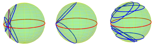
Figure 1. Small circles: $\mathcal{K}(z)=k_{0}\,z+c,\ k_{0}>0$;
$0\leq|c|<1$ (left), $c=\pm 1$ (center), $1<|c|<\sqrt{1+k_{0}^{2}}$ (right).

For instance, if $c=0$ and writing $k_{0}=\sinh\delta$, we arrive (up to rotations around the $z$-axis) at the small circle $\eta_{\delta}\equiv y=\tanh\delta$ of Example 2.5. Theorem 3.1 ensures that $\eta_{\delta}$ is the only spherical curve, up to rotations around the $z$-axis, with spherical angular momentum $\mathcal{K}(z)=\sinh\delta\,z$, $\delta>0$.

In conclusion, as a consequence of Theorem 3.1, we have proved the following uniqueness result.

Corollary 3.4.

The spherical non-parallel circles of constant curvature $k_{0}\geq 0$ are the only spherical curves (up to rotations around the $z$-axis) with spherical angular momentum $\mathcal{K}(z)=k_{0}z+c$, $|c|<\sqrt{1+k_{0}^{2}}$.

3.2. Spherical catenaries

The spherical catenaries are the equilibrium lines of an inelastic flexible homogeneous infinitely thin massive wire included in a sphere, placed in a uniform gravitational field. Like any catenaries, their centres of gravity have the minimal altitude among all the curves with given length passing by two given points. They were studied by Bobillier in 1829 and by Gudermann in 1846. Using cylindrical coordinates $(r,\theta,z)$ in $\mathbb{R}^{3}$, they can be described analytically (cf. [F93]) by the following first integral of the corresponding ordinary differential equation:

(3.7) $$(z-z_{0})\,r^{2}\,\frac{d\theta}{ds}={\rm constant}.$$

On the other hand, we study in this section spherical curves with curvature

(3.8) $$\kappa(z)=c/z^{2},\ c>0.$$

We follow Remark 3.2 considering (3.8) and choosing

(3.9) $$\mathcal{K}(z)=-\frac{c}{z},\ c>0.$$

We point out that it is the same choice of momentum as for the catenaries of $\mathbb{R}^{2}$ (see [CCI16]) and of $\mathbb{L}^{2}$ (see [CCI18]). Then we have:

(3.10) $$s=s(z)=\int\frac{z\,dz}{\sqrt{z^{2}(1-z^{2})-c^{2}}},$$

which implies that $c<1/2$ and $1-\sqrt{1-4c^{2}}<2z^{2}<1+\sqrt{1-4c^{2}}$, and it is not difficult to get:

(3.11) $$z(s)=\sqrt{\frac{1+\sqrt{1-4c^{2}}\sin 2s}{2}}.$$

We observe from (3.11) that the limit case $c=1/2$ leads to the parallel $z=1/\sqrt{2}$. In addition, we have from (3.9) that

(3.12) $$d\lambda=\frac{c}{z(1-z^{2})}\,ds$$

Looking at (3.7), taking into account that $r^{2}+z^{2}=1$ and $\theta=\lambda$, we deduce from (3.12) that we get a spherical catenary (with $z_{0}=0$ and constant $c\in(0,1/2)$). Combining (3.8) and (3.11), we have that the intrinsic equation of the spherical catenaries is given by

$$\kappa(s)=\frac{2c}{1+\sqrt{1-4c^{2}}\sin 2s},\ 0<c<1/2.$$

Now we study when the spherical catenaries are closed curves. We put $2c=\sin\beta$, with $0<\beta<\pi/2$, and call $\mathcal{C}_{\beta}$ the corresponding catenary. We have that (3.11) is rewritten as

(3.13) $$z_{\beta}(s)=\sqrt{\frac{1+\cos\beta\sin 2s}{2}}.$$

Hence $\sin(\beta/2)<z(s)<\cos(\beta/2)$. From (3.12) and (3.13), we deduce

(3.14) $$\lambda_{\beta}(s)=\int_{0}^{s}\frac{\sqrt{2}\sin\beta\,dt}{(1-\cos\beta\sin(2t))\sqrt{1+\cos\beta\sin(2t)}}.$$

Notice that $\lambda_{\beta}$ is an increasing function. Further, since the function $z_{\beta}$ is $\pi$-periodic, the catenary $\mathcal{C}_{\beta}$ will be a closed curve if and only if $\lambda_{\beta}(s+m\pi)=\lambda_{\beta}(s)+2k\pi$, with $m,k\in\mathbb{Z}$. As $\lambda_{\beta}^{\prime}$ is also a $\pi$-periodic function, $\lambda_{\beta}(s+m\pi)=\lambda_{\beta}(s)+m\lambda_{\beta}(\pi)$. Thus $\mathcal{C}_{\beta}$ is a closed curve if and only if

(3.15) $$T(\beta):=\frac{\lambda_{\beta}(\pi)}{2\pi}\in\mathbb{Q}.$$

So the problem of being $\mathcal{C}_{\beta}$ a closed curve can be solved analysing the function $T=T(\beta)$, $\beta\in(0,\pi/2)$, given in (3.15). Using the same arguments as in [Ot70], [AL15] or [Pr16], it can be proved that $T$ is a monotonically increasing function and $T((0,\frac{\pi}{2}))=(\frac{1}{2},\frac{\sqrt{2}}{2})$. Hence, for any $q\in\mathbb{Q}\cap(\frac{1}{2},\frac{\sqrt{2}}{2})$, there exists an unique $\beta_{q}\in(0,\frac{\pi}{2})$, such as $\mathcal{C}_{\beta_{q}}$ is a closed catenary. Moreover, all these closed catenaries possess dihedral symmetry, i.e. the curve can be decomposed as the union of a fundamental piece and a finite number of rotations of the fundamental piece in the sphere. The embeddedness of $\mathcal{C}_{\beta}$ would occur only if $T(\beta)=1/m$, for some positive $m\in\mathbb{Z}$. Thus the spherical catenaries are not simple curves. As a summary, the spherical catenaries consists of a sequence of undulations joining alternatively two parallels which are images of each other by rotations around the $z$-axis. They are either closed or dense in the zone between two parallels (see Figure 2). Using the nomenclature of [AGM03], we remark that the catenaries are generalized $\frac{1}{2}$-elastic curves (see Proposition 9 in [AGM03]), that is, critical points of the functional $\int_{\xi}\kappa^{1/2}\,ds$.

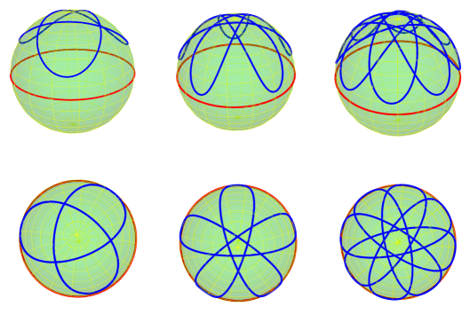
Figure 2. Two sights of the spherical catenaries $\mathcal{C}_{\beta_{2/3}}$ (left), $\mathcal{C}_{\beta_{3/5}}$ (center) and $\mathcal{C}_{\beta_{5/8}}$ (right).

In conclusion, as a consequence of Theorem 3.1, we have proved the following uniqueness result.

Corollary 3.5.

The spherical catenaries $\mathcal{C}_{\beta}$, $0<\beta<\pi/2$, are the only spherical curves (up to rotations around the $z$-axis) with spherical angular momentum $\mathcal{K}(z)=-\sin\beta/(2z)$. In addition, the closed catenaries are non-embedded, posses dihedral symmetry and can be parametrized as $\mathcal{C}_{\beta_{q}}$, with $q\in\mathbb{Q}\cap(\frac{1}{2},\frac{\sqrt{2}}{2})$.

Definition 3.6.

We denote by $\mathrm{Cat}_{\beta}$ the rotational surface $X^{0}(\mathcal{C}_{\beta})$ in $\mathbb{S}^{3}$ generated by the spherical catenary $\mathcal{C}_{\beta}$, $\beta\in(0,\pi/2)$. They will be referred to as spherical catenoids.

They coincide with the minimal rotational surfaces studied by do Carmo and Dajczer in [dCD83] and Ripoll in [Ri89]. They will play a key role in Section 5.

4. Prescribing curvature for a helicoidal surface in $\mathbb{S}^{3}$

Following the ideas of Section 2, three geometric elements determine a helicoidal surface in $\mathbb{S}^{3}$: the translation $\psi_{a}(t)$ along the fixed geodesic $c_{0}$, the rotation $\phi_{b}(t)$ around $c_{0}$ and the profile spherical curve $\xi$. But, taking into account Remark 2.1, only the pitch $h=a/b\geq 0$ and the profile curve $\xi$ are essential. As a consequence of Theorem 3.1 and the fact that rotations around the $z$-axis are nothing but translations along $c_{0}$, we conclude immediately the following interesting result.

Corollary 4.1.

Given $h\geq 0$, any helicoidal surface $X^{h}(\xi)$ in $\mathbb{S}^{3}$ is uniquely determined, up to translations along $c_{0}$, by the spherical angular momentum $\mathcal{K}=\mathcal{K}(z)$ of its profile curve $\xi=(x,y,z)$, being $z>0$ non constant.

Remark 4.2.

Corollary 4.1 means that, apart from the standard tori (see Example 2.4) corresponding to $z$ constant, any helicoidal surface in the 3-sphere is characterized by its pitch $h=a/b\geq 0$ and the spherical angular momentum $\mathcal{K}=\mathcal{K}(z)$ of its profile curve.

For instance, Lawson spherical helicoids $X^{h}(\zeta_{\pi/2})$ described in Example 2.3, are uniquely determined by $h>0$ and null spherical angular momentum $\mathcal{K}\equiv 0$ (see Corollary 3.4 and Example 3.3).

On the other hand, the totally umbilical spheres $X^{0}(\eta_{\delta})$, $\delta\geq 0$, of radius $R_{\delta}=\operatorname{sech}\delta$ (see Example 2.5) are uniquely determined by $h=0$ and linear spherical angular momentum $\mathcal{K}(z)=k_{0}z$, $k_{0}\geq 0$, being $k_{0}=\sinh\delta$ (see Corollary 3.4 and Section 3.1).

Consistent with Corollary 4.1, we are going to reveal that the geometry of the helicoidal surface $X^{h}(\xi)$, $h\geq 0$, i.e. its first and second fundamental forms, can be expressed in terms of the spherical angular momentum $\mathcal{K}=\mathcal{K}(z)$ of the profile curve $\xi=(x,y,z)$ and the non constant distance $z$ to $c_{0}$. We consider $\xi$ parameterized by the arc length $s$ and set $\xi(s)=(x(s),y(s),z(s),0)$, with $\dot{x}(s)^{2}+\dot{y}(s)^{2}+\dot{z}(s)^{2}=1$ and $z(s)>0$, $s\in I\subseteq\mathbb{R}$. For simplicity we write $X(s,t):=X^{h}(\xi)(s,t)$, see (2.2).

Denote by $g$ the induced metric of the helicoidal surface $X$. From (3.2), the entries of $g$ are given by

(4.1) $$\begin{array}[]{c}g_{11}=|X_{s}|^{2}=1,\quad g_{12}=\langle X_{s},X_{t}\rangle=-h\,\mathcal{K}(z),\vspace{0.5em}\\ \qquad g_{22}=|X_{t}|^{2}=h^{2}+(1-h^{2})z^{2}.\end{array}$$

We have that $z^{2}+\dot{z}^{2}+\mathcal{K}(z)^{2}=1$, see (3.5). Hence, a long straightforward computation provides that the unit normal $\nu$ of $X$ is given by

(4.2) $$\nu=\dfrac{1}{\alpha}\left(\nu_{1},\nu_{2},\nu_{3},\nu_{4}\right),$$

where

$$\begin{array}[]{c}\nu_{1}=z\left(-z(\dot{x}\sin ht+\dot{y}\cos ht)+\dot{z}(x\sin ht+y\cos ht)\right),\vspace{0.5em}\\ \nu_{2}=z\left(z(\dot{x}\cos ht-\dot{y}\sin ht)+\dot{z}(-x\cos ht+y\sin ht)\right),\vspace{0.5em}\\ \nu_{3}=-z\mathcal{K}(z)\cos t-h\dot{z}\sin t,\qquad\nu_{4}=-z\mathcal{K}(z)\sin t+h\dot{z}\cos t,\end{array}$$

with

(4.3) $$\alpha=\alpha(z):=\sqrt{h^{2}\dot{z}^{2}+z^{2}}=\sqrt{h^{2}(1-\mathcal{K}(z)^{2})+(1-h^{2})z^{2}}>0.$$

Notice that $\alpha^{2}=g_{11}g_{22}-g_{12}^{2}$. Hence, since $\kappa=\det(\xi,\dot{\xi},\ddot{\xi})$, we get that the entries of the second fundamental form of $X$ are given by

(4.4) $$\begin{array}[]{c}\sigma_{11}=\langle X_{ss},\nu\rangle=\dfrac{zk(z)}{\alpha(z)}=\dfrac{z\mathcal{K}^{\prime}(z)}{\alpha(z)},\quad\sigma_{12}=\langle X_{st},\nu\rangle=\dfrac{h(1-\mathcal{K}(z)^{2})}{\alpha(z)},\vspace{0.5em}\\ \qquad\sigma_{22}=\langle X_{tt},\nu\rangle=\dfrac{(1-h^{2})z^{2}\mathcal{K}(z)}{\alpha(z)}.\end{array}$$

From (4.4), we deduce that the mean curvature $H$ of the surface $X$ is given by

(4.5) $$2H(z)=\dfrac{\left(h^{2}+(1-h^{2})z^{2}\right)z\,\mathcal{K}^{\prime}(z)+\left(2h^{2}(1-\mathcal{K}(z)^{2})+(1-h^{2})z^{2}\right)\mathcal{K}(z)}{\left(h^{2}(1-\mathcal{K}(z)^{2})+(1-h^{2})z^{2}\right)^{3/2}}.$$

And its Gauss curvature is $K_{\text{G}}(z)=1+K_{\text{ext}}(z)$, where the extrinsic curvature is

(4.6) $$K_{\text{ext}}(z)=\dfrac{(1-h^{2})z^{3}\,\mathcal{K}(z)\mathcal{K}^{\prime}(z)-h^{2}(1-\mathcal{K}(z)^{2})^{2}}{\left(h^{2}(1-\mathcal{K}(z)^{2})+(1-h^{2})z^{2}\right)^{2}}.$$

Remark 4.3.

When $h=0$, using (4.1), (4.4) and (4.3), we have that $g_{12}=0=\sigma_{12}$ and $\alpha(z)=z$; that is, the coordinate curves $X(s,\cdot)$ and $X(\cdot{,t})$ are curvature lines. Therefore, the principal curvatures of a rotational surface $X^{0}(\xi)$ in $\mathbb{S}^{3}$ are given by $\kappa_{i}=\sigma_{ii}/g_{ii}$, $i=1,2$, that is:

(4.7) $$\kappa_{1}(z)=\mathcal{K}^{\prime}(z),\ \kappa_{2}(z)=\frac{\mathcal{K}(z)}{z}.$$

When $h=1$, using (4.6), we clearly have that $K_{\text{ext}}\equiv-1$ and then we obtain that the Hopf immersions $X^{1}(\xi)$ (see Remark 2.2) are flat, that is, $K_{\text{G}}\equiv 0$.

Inspired by [BK98], we show in the next result that if we prescribe the mean curvature $H$ or the extrinsic curvature $K_{\text{ext}}$ (or, equivalently, the Gauss curvature $K_{\text{G}}$) of a helicoidal surface $X^{h}(\xi)$ by means of a function $H=H(z)$ or $K_{\text{ext}}=K_{\text{ext}}(z)$ respectively, we can determine the spherical angular momentum $\mathcal{K}(z)$ of the profile curve $\xi=(x,y,z)$ and, as a consequence of Corollary 4.1, the helicoidal surface $X^{h}(x,y,z)$ up to translations along the fixed geodesic $c_{0}$.

Theorem 4.4.

1. Given $h\geq 0$, let $H=H(z)$, $z>0$, be a continuous function. Then there exists a one-parameter family of helicoidal surfaces with pitch $h$ in $\mathbb{S}^{3}$ and mean curvature $H(z)$, uniquely determined, up to translations along $c_{0}$, by the spherical angular momenta of their profile curves given by

   (4.8) $$\mathcal{K}(z)=\pm\dfrac{\sqrt{h^{2}+(1-h^{2})z^{2}}A(z)}{\sqrt{1+h^{2}A(z)^{2}}},$$

   where

   (4.9) $$z^{2}A(z)=2\!\int\!zH(z)dz.$$

2. Given $h\geq 0$, $h\neq 1$, let $K_{\text{ext}}=K_{\text{ext}}(z)$, $z>0$, be a continuous function. Then there exists a one-parameter family of helicoidal surfaces with pitch $h$ in $\mathbb{S}^{3}$ and extrinsic curvature $K_{\text{ext}}(z)$, uniquely determined, up to translations along $c_{0}$, by the spherical angular momenta of their profile curves given by

   (4.10) $$\mathcal{K}(z)=\pm\sqrt{1+\dfrac{(1-h^{2})z^{2}B(z)}{z^{2}+h^{2}B(z)}},$$

   where

   (4.11) $$B(z)=2\!\int\!zK_{\text{ext}}(z)dz.$$

Remark 4.5.

The parameter in both uniparametric families described in Theorem 4.4 comes from the integration constant in (4.9) and (4.11).

Proof.

First, given $h\geq 0$ and a profile curve $\xi$, for any helicoidal surface $X=X^{h}(\xi)$ we define

$$A(z):=\frac{\mathcal{K}(z)}{\left(h^{2}(1-\mathcal{K}(z)^{2})+(1-h^{2})z^{2}\right)^{1/2}},$$

where $\mathcal{K}(z)$ is the spherical angular momentum of $\xi$; note that $A(z)$ is well defined by (4.3). Then we deduce that (4.5) can be written as

(4.12) $$2H(z)=zA^{\prime}(z)+2A(z).$$

Assume now that the mean curvature of $X$ is prescribed by a continuous function $H=H(z)$, $z>0$. We can interpret (4.12) as the linear ordinary differential equation

$$A^{\prime}(z)+\frac{2}{z}A(z)=\frac{2H(z)}{z}$$

that $A=A(z)$ must satisfy, whose general solution is given in (4.9). From the definition of $A=A(z)$, we arrive at (4.8), which is also well defined by (4.3).

On the other hand, given $h\geq 0$ and a profile curve $\xi$, for any helicoidal surface $X=X^{h}(\xi)$ we consider the well defined non positive function (see (4.3)) given by

$$B(z):=-\frac{z^{2}(1-\mathcal{K}(z)^{2})}{h^{2}(1-\mathcal{K}(z)^{2})+(1-h^{2})z^{2}}\leq 0.$$

Here, equation (4.6) is rewritten as

(4.13) $$B^{\prime}(z)=2zK_{\text{ext}}(z).$$

If we assume that the extrinsic curvature of $X$ is prescribed by a continuous function $K_{\text{ext}}=K_{\text{ext}}(z)$, we read (4.13) with unknown $B=B(z)$ and its solution is given in (4.11). Using the definition of $B=B(z)$, a direct computation gives us (4.10) if $h\neq 1$, which is also well defined by (4.3). ∎

5. Rotational and helicoidal minimal surfaces in $\mathbb{S}^{3}$

In order to study helicoidal (in particular, rotational) minimal surfaces in $\mathbb{S}^{3}$, given $h\geq 0$, we prescribe $H\equiv 0$ in Theorem 4.4. Thus, $A(z)=c/z^{2}$, $c\in\mathbb{R},$ and we get a one-parameter family of minimal helicoidal surfaces with pitch $h$, determined by the family of spherical angular momenta of (4.8) given by

(5.1) $$\mathcal{K}^{h}_{c}(z)=\pm\frac{c\sqrt{h^{2}+(1-h^{2})z^{2}}}{\sqrt{z^{4}+h^{2}c^{2}}}.$$

Recall from part (ii) in Remark 3.2 that it is necessary that $z^{2}+\mathcal{K}^{h}_{c}(z)^{2}<1$. Using (5.1), it is not difficult to check that this condition is equivalent to $z^{4}+c^{2}<z^{2}$. Writing $z=\sin\varphi$, we have that $c^{2}<z^{2}(1-z^{2})=\sin^{2}\varphi\cos^{2}\varphi=\frac{1}{4}\sin^{2}2\varphi<\frac{1}{4}$. In addition, from (5.1) it is clear that $\mathcal{K}^{h}_{-c}=-\mathcal{K}^{h}_{c}$ and then it is enough to consider $c\geq 0$. Hence, we take $c\in[0,1/2)$. We point out that, up to a change of orientation, we can choose the sign $\pm$ we want. We introduce now some notation. For any $h\geq 0$ and $0\leq c<1/2$, we denote by $\mathrm{Hel}_{c}^{h}$ the corresponding family of helicoidal minimal surfaces determined by (5.1) according to Theorem 4.4, choosing minus sign. Summarizing this reasoning, we get the following result.

Corollary 5.1.

Given $h\geq 0$, the helicoidal minimal surfaces of pitch $h$ in $\mathbb{S}^{3}$ are described by the one parameter family $\mathrm{Hel}_{c}^{h}:=X^{h}(\xi_{c}^{h})$, $0\leq c<1/2$, uniquely determined, up to translations along $c_{0}$, by the spherical angular momenta

(5.2) $$\mathcal{K}^{h}_{c}(z)=-\frac{c\,\sqrt{h^{2}+(1-h^{2})z^{2}}}{\sqrt{z^{4}+h^{2}c^{2}}},\ 0\leq c<1/2,$$

of their profile curves $\xi_{c}^{h}$.

5.1. Rotational minimal surfaces in $\mathbb{S}^{3}$

We start studying the rotational case corresponding to $h=0$. From (5.2), we arrive at $\mathcal{K}^{0}_{c}(z)=-c/z$, with $c\in[0,1/2)$. The previous study done in Section 3.2 allows us to provide the following local classification theorem, where we summarize and easily prove results from [AL15], [Br13c], [dCD83], [Ot70], [Pr16] and [Ri89] concerning minimal rotational surfaces in $\mathbb{S}^{3}$. In addition, from a global point of view, we also identify the Otsuki tori and the Brendle-Kusner tori and characterize them according to [Br13c].

Theorem 5.2.

The only rotational minimal surfaces in $\mathbb{S}^{3}$ are open subsets of the following surfaces:

1. The totally geodesic sphere $\mathbb{S}^{2}\hookrightarrow\mathbb{S}^{3}$.

2. The Clifford torus $\mathbb{S}^{1}(1/\sqrt{2})\times\mathbb{S}^{1}(1/\sqrt{2})\hookrightarrow\mathbb{S}^{3}$.

3. The spherical catenoids $\mathrm{Cat}_{\beta}$, $0<\beta<\pi/2$ (see Definition 3.6).

Furthermore, the compact spherical catenoids $\mathrm{Cat}_{\beta_{q}}=X^{0}(\mathcal{C}_{\beta_{q}})$, $q\in\mathbb{Q}\cap(\frac{1}{2},\frac{\sqrt{2}}{2})$ (see Corollary 3.5 and Definition 3.6), are exactly the Otsuki tori, which also agree with the Brendle-Kusner tori. Joint with the Clifford torus, they are the only Alexandrov immersed minimal tori in $\mathbb{S}^{3}$.

Remark 5.3.

Brendle showed, pointed by Kusner (see [Br13b, Theorem 1.4]) that there exists an infinite family of minimal tori in $\mathbb{S}^{3}$ which are Alexandrov immersed, but fail to be embedded. In particular, we are going to prove that they are nothing but the so-called Otsuki tori (see [Ot70, HS12]). Moreover, he proved in [Br13c] that any minimal torus in $\mathbb{S}^{3}$ which is Alexandrov immersed must be rotationally symmetric.

On the other hand, Brendle solved Lawson Conjecture affirmatively proving in [Br13a] that the Clifford torus is the only embedded minimal torus in $\mathbb{S}^{3}$. In this line, we conclude in Theorem 5.2 that the compact spherical catenoids, which coincide with the Otsuki and Brendle-Kusner tori, are the only Alexandrov immersed minimal tori in $\mathbb{S}^{3}$.

We use (3.13) and (3.14) in the parametrization (2.3) composed with a stereographic projection into $\mathbb{R}^{3}$ to visualize some of these tori in Figure 3.

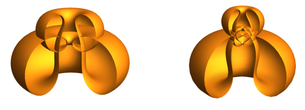
Figure 3. Open sights (with $t\in(0,3\pi/2)$) of the Otsuki-Brendle-Kusner spherical catenoids $\mathrm{Cat}_{\beta_{2/3}}$ and $\mathrm{Cat}_{\beta_{3/5}}$.

Proof of Theorem 5.2.

We are going to use Corollary 5.1 with $h=0$. But first, we must have into account the case that $z$ is constant, see Corollary 4.1. We know that this corresponds to the standard tori (see Example 2.4), which are CMC surfaces and only the Clifford torus is minimal. This leads to case (ii).

Next, we determine the surfaces $\mathrm{Hel}_{c}^{0}$ through $\mathcal{K}^{0}_{c}(z)=-c/z$, with $c\in[0,1/2)$. If $c=0$, we get that $\mathcal{K}\equiv 0$ and we arrive at case (i), see Remark 4.2. If $c\neq 0$, we proceed as in Section 3.2 and Corollary 3.5 and Definition 3.6 gives us case (iii), since $\mathrm{Cat}_{\beta}=X^{0}(\mathcal{C}_{\beta})$, $\beta\in(0,\pi/2)$, is exactly $\mathrm{Hel}_{c}^{0}$, with $c=\frac{1}{2}\sin\beta$.

On the other hand, Brendle-Kusner tori are described in the following way (see [Br13b, Theorem 1.4] for more details). Consider an immersion of the form

$$F(t,\theta)=\left(r(t)\,e^{it},\sqrt{1-r(t)^{2}}\,e^{i\theta}\right),$$

where $r(t)$ is a smooth function taking values in the interval $(0,1)$ and satisfying the following differential equation for some constant $C\in(0,1)$:

(5.3) $$\frac{r^{\prime 2}}{r^{4}(1-r^{2})}+\frac{1}{r^{2}(1-r^{2})}=\frac{4}{C^{2}}.$$

It turns to be that $F$ is doubly periodic under certain rationality condition involving the constant $C$ and the interval $(1/2,\sqrt{2}/2)$. Now we consider the spherical curve given by $\xi(t)=\left(r(t)\cos t,r(t)\sin t,\sqrt{1-r(t)^{2}}\right)$. We have that $|\xi^{\prime}|^{2}=\frac{r^{\prime 2}+r^{2}(1-r^{2})}{1-r^{2}}$. Now we write $r(t)=\cos\varphi(s)=\sqrt{1-z(s)^{2}}$ through the change of variable $t=\lambda(s)$ given by (3.12). Then it is not difficult to check that (5.3) is satisfied if and only if $C=\sin\beta$, where $\beta\in(0,\pi/2)$ is the corresponding parameter of the spherical catenoid $\mathrm{C}at_{\beta_{q}}$, and the aforementioned rationality condition on $C$ is exactly (3.15). The Clifford torus corresponds to the constant solution $r=z=1/\sqrt{2}$, that is, the limiting case $\beta=\pi/2$.

To finish the proof, let us prove that Otsuki tori also coincide with the spherical catenoids described in Definition 3.6. We follow the description of Otsuki tori given in [HS12]. For any $\alpha\in[0,2\pi)$, Otsuki tori are of the form

$$\big{(}\mathcal{H(\theta)}\cos\alpha,\mathcal{H(\theta)}\sin\alpha,u(\theta),v(\theta)\big{)},$$

with $\mathcal{H(\theta)}:=\sqrt{1-h(\theta)^{2}-h^{\prime}(\theta)^{2}}$, $u(\theta):=h(\theta)\sin\theta+h^{\prime}(\theta)\cos\theta$, $v(\theta):=h^{\prime}(\theta)\sin\theta-h(\theta)\cos\theta$ and where the support function $h=h(\theta)\in(0,1)$ is a non-constant periodic solution to the IVP given by

$$2h(1-h^{2})h^{\prime\prime}+h^{\prime 2}(1-h^{2})(2h^{2}-1)=0,\quad 0<h(0)\leq\frac{1}{\sqrt{2}},\quad h^{\prime}(0)=0.$$

We are able to find out a first integral to the above ODE. Concretely:

(5.4) $$\frac{h(1-h^{2}-h^{\prime 2})}{\sqrt{1-h^{2}}}=c,$$

for some constant $c\in\mathbb{R}$ depending on $h(0)$. It is clear that we are dealing with $X^{0}(\xi)$, where $\xi=\xi(\theta)$ is the spherical curve given by $\xi(\theta)=(u(\theta),v(\theta),\mathcal{H(\theta)})$. We compute its spherical angular momentum and obtain that

$$\mathcal{K}(\theta)=-h(\theta)\sqrt{\frac{1-h(\theta)^{2}-h^{\prime}(\theta)^{2}}{1-h(\theta)^{2}}}.$$

Taking into account (5.4) and that $z(\theta)=\mathcal{H(\theta)}=\sqrt{1-h(\theta)^{2}-h^{\prime}(\theta)^{2}}$, we deduce that $\mathcal{K}(z)=-c/z$. Using Corollary 4.1, Corollary 3.5 and Definition 3.6 we conclude the result. ∎

5.2. Helicoidal minimal surfaces in $\mathbb{S}^{3}$

We go on by studying the proper helicoidal minimal surfaces $\mathrm{Hel}_{c}^{h}$ in $\mathbb{S}^{3}$, corresponding to $h>0$ (and $0\leq c<1/2$) in Corollary 5.1. We emphasize that, using Remark 4.2, they provide a deformation by helicoidal minimal surfaces of the Lawson spherical helicoids $\mathrm{Hel}_{0}^{h}$ corresponding to $c=0$. Moreover, one may easily check that for any $h>0$, the Lawson helicoids $\mathrm{Hel}_{0}^{h}$ and $\mathrm{Hel}_{0}^{1/h}$ are congruent and the Clifford torus corresponds to $\mathrm{Hel}_{0}^{1}$, see Example 2.3-(ii).

On the other hand, recall that for any $\beta\in(0,\pi/2)$, $\mathrm{Cat}_{\beta}$ is the spherical catenoid $X^{0}(\mathcal{C}_{\beta})$ (see Definition 3.6). Note that $\mathrm{Cat}_{\beta}=\mathrm{Hel}_{c}^{0}$, when $c=\frac{1}{2}\sin\beta$. In the following result we match spherical catenoids and Lawson spherical helicoids from a local isometric point of view.

Theorem 5.4.

Any spherical catenoid is locally isometric to two, and only two, Lawson spherical helicoids. Concretely, the catenoid $\mathrm{Cat}_{\beta}$, $\beta\in(0,\pi/2)$, is locally isometric to the helicoids $\mathrm{Hel}^{\tan(\beta/2)}_{0}$ (with pitch less than one) and $\mathrm{Hel}^{\cot(\beta/2)}_{0}$ (with pitch greater than one).

Remark 5.5.

Recall that the limiting case $\beta=\pi/2$ degenerates into the Cliford torus $\mathrm{Hel}^{1}_{0}\equiv\mathrm{Cat}_{\pi/2}$.

Proof of Theorem 5.4.

From formulae (4.1) for the induced metric of a helicoidal surface and equations (3.13) and (2.5), we may compute the first fundamental form of both $\mathrm{Cat}_{\beta}$ and $\mathrm{Hel}^{h}_{0}$. For $\mathrm{Cat}_{\beta}$, $\beta\in(0,\pi/2)$, the first fundamental form $I$, in coordinates $(s,t)$, is given by

(5.5) $$I=ds^{2}+\frac{1+\cos\beta\sin 2s}{2}dt^{2},$$

and for $\mathrm{Hel}^{h}_{0}$, $h>0$, the first fundamental form $\tilde{I}$, in coordinates $(\tilde{s},\tilde{t})$, is

(5.6) $$\tilde{I}=d\tilde{s}^{2}+(h^{2}\cos^{2}\tilde{s}+\sin^{2}\tilde{s})d\tilde{t}^{2}.$$

For simplicity, we denote by $Y_{\beta}$ the corresponding parametrization of $\mathrm{Cat}_{\beta}$ and by $Y^{h}$ the one of $\mathrm{Hel}_{0}^{h}$. We define the map $\Phi:=Y^{h}\circ\phi\circ(Y_{\beta})^{-1}$ from $\mathrm{Cat}_{\beta}\equiv Y_{\beta}(s,t)$ to $\mathrm{Hel}^{h}_{0}\equiv Y^{h}(\tilde{s},\tilde{t})$, where

$$(\tilde{s},\tilde{t})=\phi(s,t)=\left(s\pm\frac{\pi}{4},\frac{t}{\sqrt{1+h^{2}}}\right),$$

the sign $\pm$ according to $h\lessgtr 1$. Then, using (5.6), we get that

$$\tilde{I}=ds^{2}+\frac{1}{2}\left(1\pm\frac{1-h^{2}}{1+h^{2}}\sin 2s\right)dt^{2}.$$

Looking at (5.5), we must take

(5.7) $$\cos\beta=\frac{1-h^{2}}{1+h^{2}}\ \text{ if }\ h<1,\quad\text{ or }\quad\cos\beta=\frac{h^{2}-1}{1+h^{2}}\ \text{ if }\ h>1,$$

in order to get $\tilde{I}=I$ and so $\Phi$ is the desired local isometry. The case $h=1$ corresponds to the Clifford torus (see Remark 5.5). We point out that (5.7) provides a monotonically decreasing correspondence $h\in(0,1)\mapsto\beta\in(0,\pi/2)$, and a monotonically increasing correspondence $h\in(1,\infty)\mapsto\beta\in(0,\pi/2)$, whose inverse maps are precisely $h=\tan(\beta/2)$ and $h=\cot(\beta/2)$ respectively. This finishes the proof. ∎

We now aim to identify the surfaces $\mathrm{Hel}_{c}^{h}$, $0\leq c<1/2$, $h>0$, $h\neq 1$, in terms of the associated surfaces (in the sense defined in [La70, Section 13]) of a given spherical catenoid $\mathrm{Cat}_{\beta}$, $\beta\in(0,\pi/2)$. For this purpose, recall the following fact, coming from the proof of [La70, Theorem 8]:

For any minimal immersion $X\colon S\rightarrow\mathbb{S}^{3}$ of a simply connected surface $S$, there exists a differentiable, $2\pi$–periodic family of minimal isometric immersions $X_{\theta}\colon S\rightarrow\mathbb{S}^{3}$. Moreover, up to congruences, the maps $X_{\theta}$, $0\leq\theta\leq\pi$, represent (extensions of) all local, isometric, minimal immersions of $S$ into $\mathbb{S}^{3}$. The surface $X_{\pi/2}$ is called the conjugate surface of $X$.

To introduce in practice the family of associated surfaces, we proceed as described also in [dCD83]: Let $(x,y)$ be isothermal coordinates for the minimal immersion $X:S\rightarrow\mathbb{S}^{3}$. Denote by $I=E(dx^{2}+dy^{2})$ and $I\!I=\sigma_{11}dx^{2}+2\sigma_{12}dxdy+\sigma_{22}dy^{2}$ the first and second fundamental forms of $X$, respectively. Set $\psi=\sigma_{11}-i\sigma_{12}$ and define a family of quadratic forms depending on a parameter $\theta\in[0,2\pi]$ by

$$\sigma_{11}(\theta)={\rm Re}(e^{i\theta}\psi),\ \sigma_{12}(\theta)={\rm Im}(e^{i\theta}\psi),\ \sigma_{22}(\theta)=-{\rm Re}(e^{i\theta}\psi).$$

Then $I_{\theta}=I$ and $I\!I_{\theta}=\sigma_{11}(\theta)dx^{2}+2\sigma_{12}(\theta)dxdy+\sigma_{22}(\theta)dy^{2}$ satisfy the Gauss and Codazzi equations, thus giving rise to the isometric family $X_{\theta}:S\rightarrow\mathbb{S}^{3}$ of minimal immersions. The immersion $X_{\pi/2}$ is the conjugate immersion to $X_{0}=X$.

We are now able to prove in detail the following result commented in [dCD83, Remark 3.34].

Theorem 5.6.

Given a spherical catenoid $\text{Cat}_{\beta}$, $\beta\in(0,\pi/2)$, the associated immersions $(\text{Cat}_{\beta})_{\theta}$, $0\leq\theta\leq\pi$, coincide with the helicoidal minimal immersions $\mathrm{Hel}_{c}^{h}$, $0\leq c<1/2$, $h\geq 0$, $h\neq 1$, where

(5.8) $$\frac{(1-h^{2})^{2}c^{2}+h^{2}}{(1+h^{2})^{2}}=\frac{\sin^{2}\beta}{4},\qquad\cos\theta=\frac{c(1-h^{2})}{\sqrt{(1-h^{2})^{2}c^{2}}+h^{2}}.$$

In particular, the conjugate surface of the spherical catenoid $\text{Cat}_{\beta}=(\text{Cat}_{\beta})_{0}$ is the Lawson spherical helicoid $\mathrm{Hel}_{0}^{h}=(\text{Cat}_{\beta})_{\pi/2}$, with $\frac{h^{2}}{(1+h^{2})^{2}}=\frac{\sin^{2}\beta}{4}$.

Remark 5.7.

Bearing in mind Theorem 5.4, it is easy to check that $h^{2}/(1+h^{2})^{2}=\frac{1}{4}\sin^{2}\beta$ if, and only if, $h=\tan\beta/2$ or $h=\cot\beta/2$. In Figure 4, we draw in the region $0\leq c<1/2$, $h\geq 0$, the curves $c_{\beta}$ given by

$$c_{\beta}\equiv\frac{(1-h^{2})^{2}c^{2}+h^{2}}{(1+h^{2})^{2}}=\frac{\sin^{2}\beta}{4}$$

for different values of $\beta\in(0,\pi/2)$. Each curve $c_{\beta}$ has two connected components separated by the line $h=1$.

It is not difficult to deduce from (5.8) that $\theta=0\Leftrightarrow c=\frac{1}{2}\sin\beta$, $h=0$; $\theta\in(0,\pi/2)\Leftrightarrow h<1$; $\theta=\pi/2\Leftrightarrow c=0$, $h=\tan\beta/2$ or $h=\cot\beta/2$; and $\theta\in(\pi/2,\pi)\Leftrightarrow h>1$.

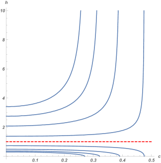
Figure 4. Representation of the associated immersions to a spherical catenoid.

Remark 5.8.

The immersions $\mathrm{Hel}_{c}^{1}$, $0\leq c<1/2$, are Hopf minimal surfaces in $\mathbb{S}^{3}$ (see Remark 4.3), so they are flat. Using a classical result in [La69], all of them provide representations of the Clifford torus $\mathrm{Hel}_{0}^{1}$ as helicoidal surfaces.

Proof of Theorem 5.6.

Let $\mathrm{Cat}_{\beta}$, $\beta\in(0,\pi/2)$, be the spherical catenoid given in Definition 3.6 and let $(\mathrm{Cat}_{\beta})_{\theta}$, $\theta\in(0,\pi)$, be its associated immersions. Let $(\tilde{s},\tilde{t})$ be the local coordinates for the catenoid $\mathrm{Cat}_{\beta}$ given by (2.3) when the generatrix curve is the spherical catenary $\mathcal{C}_{\beta}$ studied in Section 3.2. In order to define the associated immersions as in [La70, Section 13] we take isothermal coordinates $(x,y)$ defined by

(5.9) $$dx=\frac{1}{\tilde{z}(\tilde{s})}d\tilde{s},\quad dy=d\tilde{t},$$

where $\tilde{z}=\tilde{z}_{\beta}$ is given by (3.13). In such new coordinates, using (4.1), (4.4) and (3.9), the coefficients of the first fundamental form $\widetilde{g}$ and the second fundamental form $\widetilde{\sigma}$ of $(\mathrm{Cat}_{\beta})_{\theta}$, $0\leq\theta<\pi$, are expressed by

(5.10) $$\widetilde{g}_{xx}=\widetilde{g}_{yy}=\tilde{z}^{2},\quad\widetilde{g}_{xy}=0,$$

and

(5.11) $$\widetilde{\sigma}_{xx}=\frac{1}{2}\sin\beta\cos\theta,\quad\widetilde{\sigma}_{xy}=\frac{1}{2}\sin\beta\sin\theta,\quad\widetilde{\sigma}_{yy}=-\frac{1}{2}\sin\beta\cos\theta.$$

Let now $(s,t)$ be the local coordinates for the helicoidal surfaces $\mathrm{Hel}_{c}^{h}$, $0\leq c<1/2$ and $h\geq 0$, $h\neq 1$, given by (2.2) when the profile curves are the spherical curves $\xi^{h}_{c}$ described in Corollary 5.1.

Next we are going to use coordinates $(\tilde{z},\tilde{t})$ for $(\mathrm{Cat}_{\beta})_{\theta}$ and $(z,t)$ for $\mathrm{Hel}_{c}^{h}$, where $\tilde{z}$ and $z$ come from (3.5) when $\mathcal{K}(\tilde{z})$ and $\mathcal{K}(z)$ are respectively given in (3.9) and (5.2).

We define a map $\Phi$ given by $(\tilde{z},\tilde{t})\mapsto(z,t)$ from $(\mathrm{Cat}_{\beta})_{\theta}$ onto $\mathrm{Hel}_{c}^{h}$ such that

(5.12) $$\tilde{z}(z)=\sqrt{\frac{(1-h^{2})z^{2}+h^{2}}{1+h^{2}}}$$

and

(5.13) $$d\tilde{t}=\frac{hc\sqrt{1+h^{2}}}{z\,\sqrt{(1-h^{2})z^{2}+h^{2}}\,\sqrt{z^{2}-z^{4}-c^{2}}}\,dz+\sqrt{1+h^{2}}\,dt,\ \text{if $0<h<1$},$$

or

(5.14) $$d\tilde{t}=-\frac{hc\sqrt{1+h^{2}}}{z\,\sqrt{(1-h^{2})z^{2}+h^{2}}\,\sqrt{z^{2}-z^{4}-c^{2}}}\,dz-\sqrt{1+h^{2}}\,dt,\ \text{if $h>1$}.$$

All the above changes of local parameters are summarized in the following diagram:

(5.15)

Our aim is to obtain the coefficients of the first fundamental form $g$ and the second fundamental form $\sigma$ of $\mathrm{Hel}_{c}^{h}$ in the coordinates $(x,y)$ and show that they coincide with (5.10) and (5.11) respectively when $h$, $c$, $\beta$ and $\theta$ satisfy (5.8).

Assume first that $0<h<1$. From (5.15) (using (5.13)) and taking into account (5.8), we compute the partial derivatives of $(x,y)$ with respect to $s$ and $t$, obtaining

$$x_{s}= \frac{dx}{d\tilde{s}}\frac{d\tilde{s}}{d\tilde{z}}\frac{d\tilde{z}}{dz}\frac{dz}{ds}=\frac{\sqrt{1+h^{2}}\,z^{2}}{\sqrt{h^{2}+(1-h^{2})z^{2}}\,\sqrt{c^{2}h^{2}+z^{4}}},$$

$$x_{t}= 0,$$

$$y_{s} =\frac{dy}{d\tilde{t}}\frac{d\tilde{t}}{dz}\frac{dz}{ds}=\frac{hc\sqrt{1+h^{2}}}{\sqrt{h^{2}+(1-h^{2})z^{2}}\,\sqrt{c^{2}h^{2}+z^{4}}},$$

$$y_{t} =\frac{dy}{d\tilde{t}}\frac{d\tilde{t}}{dt}=\sqrt{1+h^{2}}.$$

Denote by $g_{xx}$, $g_{xy}$ and $g_{yy}$ the coefficients of the first fundamental form of $\mathrm{Hel}_{c}^{h}$ through the parameters $(x,y)$ whilst $g_{ss}$, $g_{st}$, and $g_{tt}$ denote the entries of $g$ through the parameters $(s,t)$. A straightforward computation provides the following relation between them:

$$\begin{cases}g_{ss}=x_{s}^{2}\,g_{xx}+2x_{s}y_{s}\,g_{xy}+y_{s}^{2}\,g_{yy}\\ g_{st}=x_{s}y_{t}\,g_{xy}+y_{s}y_{t}\,g_{yy}\\ g_{tt}=y_{t}^{2}\,g_{yy}\end{cases}$$

Using (4.1) and (5.2), we get that

$$g_{xx} = \frac{1}{x_{s}^{2}}\big{(}g_{ss}-\frac{2y_{s}}{y_{t}}g_{st}+\frac{y_{s}^{2}}{y_{t}^{2}}g_{tt}\big{)}=\frac{h^{2}+(1-h^{2})z^{2}}{1+h^{2}},$$

$$g_{xy} = \frac{1}{x_{s}y_{t}}\big{(}g_{st}-\frac{y_{s}}{y_{t}}g_{tt}\big{)}=0,$$

$$g_{yy} = \frac{1}{y_{t}^{2}}g_{tt}=\frac{h^{2}+(1-h^{2})z^{2}}{1+h^{2}}.$$

From (5.12) we deduce that $g$ coincides with $\widetilde{g}$ as desired, see (5.10). This ensures that the map $\Phi$ is a local isometry. To conclude the result, we now check that the second fundamental forms of $(\mathrm{Cat}_{\beta})_{\theta}$ and $\mathrm{Hel}_{c}^{h}$ also coincide. Denote by $\sigma_{xx}$, $\sigma_{xy}$, and $\sigma_{yy}$ the coefficients of the second fundamental form of $\mathrm{Hel}_{c}^{h}$ through the parameters $(x,y)$ whilst $\sigma_{ss}$, $\sigma_{st}$, and $\sigma_{tt}$ denote the entries of $\sigma$ through the parameters $(s,t)$. We arrive at the corresponding relations:

$$\begin{cases}\sigma_{ss}=x_{s}^{2}\,\sigma_{xx}+2x_{s}y_{s}\,\sigma_{xy}+y_{s}^{2}\,\sigma_{yy},\\ \sigma_{st}=x_{s}y_{t}\,\sigma_{xy}+y_{s}y_{t}\,\sigma_{yy},\\ \sigma_{tt}=y_{t}^{2}\,\sigma_{yy},\end{cases}$$

Then, using (4.4) and (5.2) taking (5.8) into account, we obtain that

$$\sigma_{xx} = \frac{1}{x_{s}^{2}}\big{(}\sigma_{ss}-\frac{2y_{s}}{y_{t}}\sigma_{st}+\frac{y_{s}^{2}}{y_{t}^{2}}\sigma_{tt}\big{)}=c\,\frac{1-h^{2}}{1+h^{2}}=\frac{1}{2}\sin\beta\cos\theta,$$

$$\sigma_{xy} = \frac{1}{x_{s}y_{t}}\big{(}\sigma_{st}-\frac{y_{s}}{y_{t}}\sigma_{tt}\big{)}=\frac{h}{1+h^{2}}=\frac{1}{2}\sin\beta\sin\theta,$$

$$\sigma_{yy} = \frac{1}{y_{t}^{2}}\sigma_{tt}=-c\,\frac{1-h^{2}}{1+h^{2}}=-\frac{1}{2}\sin\beta\cos\theta.$$

Therefore, using the fact that surfaces are uniquely determined by their first and second fundamental forms, we can conclude that $(\mathrm{Cat}_{\beta})_{\theta}$ and $\mathrm{Hel}^{h}_{c}$ are congruent surfaces.

Assume now that $h>1$; in that case, from (5.14), we have that

$$x_{s}= -\frac{\sqrt{1+h^{2}}\,z^{2}}{\sqrt{h^{2}+(1-h^{2})z^{2}}\,\sqrt{c^{2}h^{2}+z^{4}}},$$

$$x_{t}= 0,$$

$$y_{s} =-\frac{hc\sqrt{1+h^{2}}}{\sqrt{h^{2}+(1-h^{2})z^{2}}\,\sqrt{c^{2}h^{2}+z^{4}}},$$

$$y_{t} =-\sqrt{1+h^{2}}.$$

Following similar computations using now (5.2), we reach the same expressions for the entries of the first and second fundamental forms that the corresponding to the case of $0<h<1$. Therefore we conclude again that $(\mathrm{Cat}_{\beta})_{\theta}$ and $\mathrm{Hel}^{h}_{c}$ are congruent surfaces. ∎

Remark 5.9.

In the same way that we can find compact catenoids $\mathrm{Cat}_{\beta_{q}}$, $q\in\mathbb{Q}\cap(\frac{1}{2},\frac{\sqrt{2}}{2})$ (see Definition 3.6 and Corollary 3.5), it is to be expected that the same happens in the family of minimal helicoids $\mathrm{Hel}_{c}^{h}$, $0\leq c<1/2$, $h\geq 0$, $h\neq 1$. But it is not an easy problem to determine even when their $z$-function is periodic.

References

- [AL15] B. Andrews and H. Li, Embedded constant mean curvature tori in the three-sphere, J. Diff. Geom. 99 (2015), 169–189.
- [A78] V.I. Arnold, Mathematical methods of classical mechanics, Springer Verlag, 1978.
- [AGM03] J. Arroyo, O.J. Garay and J.J. Mencía, Closed generalized elastic curves in , J. Geom. Phys. 48 (2003), 339–353.
- [BK98] C. Baikoussis and T. Koufogiorgos, Helicoidal surfaces with prescribed mean or Gaussian curvature, J. Geom. 63 (1998), 25–29.
- [Br13a] S. Brendle, Embedded minimal tori in and the Lawson Conjecture, Acta Math. 211 (2013), 177–190.
- [Br13b] S. Brendle, Minimal surfaces in : a survey of recent results, Bull. Math. Sci. 3 (2013), 133–-171.
- [Br13c] S. Brendle, Alexandrov immersed minimal tori in , Math. Res. Lett. 20 (2013), 459–-464.
- [Ca67] E. Calabi, Minimal immersions of surfaces in Euclidean spheres, J. Diff. Geom. 1 (1967), 111–127.
- [CCI16] I. Castro and I. Castro-Infantes, Plane curves with curvature depending on distance to a line, Diff. Geom. Appl. 44 (2016), 77–97.
- [CCI18] I. Castro, I. Castro-Infantes and J. Castro-Infantes, Curves in Lorentz-Minkowski plane: elasticae, catenaries and grim-reapers, Open Math. 16 (2018), 747–766.
- [dCD83] M.P. do Carmo and M. Dajczer, Rotation hypersurfaces in spaces of constant curvature, Trans. Amer. Math. Soc. 277 (1983), 685–709.
- [E11] N. Edelen, A conservation approach to helicoidal surfaces of constant mean curvature in , and , arXiv:1110.1068.
- [F93] R. Ferréol, Encyclopédie des formes mathématiques remarquables, www. mathcurve. com
- [HL71] W.Y. Hsiang and H.B. Lawson, Minimal submanifolds of low cohomogeneity, J. Diff. Geom. 5 (1971), 1–38.
- [HS12] Z. Hu and H. Song, On Otsuki tori and their Willmore energy, J. Math. Anal. Appl. 395 (2012), 465–472.
- [La69] H.B. Lawson, Local rigidity theorems for minimal hypersurfaces, Ann. of Math. 89 (1969), 187–197.
- [La70] H.B. Lawson, Complete minimal surfaces in , Ann. of Math. 92 (1970), 335–374.
- [MdS19] F. Manfio and J.P. dos Santos, Helicoidal flat surfaces in the 3-sphere, Math. Nachr. 292 (2019), 127–136.
- [MP12] W.H. Meeks and J. Pérez, A survey on classical minimal surface theory, University Lecture Series (AMS) vol. 60 (2012) 182 pages.
- [Ot70] T. Otsuki, Minimal hypersurfaces in a Riemannian manifold of constant curvature, Amer. J. Math. 92 (1970), 145–173.
- [Pn13] A.V. Penskoi, Extremal spectral properties of Otsuki tori, Math. Nachr. 286 (2013), 379–391.
- [Pr10] O.M. Perdomo, Embedded constant mean curvature hypersurfaces on spheres, Asian J. Math. 14 (2010), 73–108.
- [Pr16] O.M. Perdomo, Rotational surfaces in with constant mean curvature, J. Geom. Anal. 26 (2016), 2155–2168.
- [Ri89] J.B. Ripoll, Uniqueness of minimal rotational surfaces in , Amer. J. Math. 111 (1989), 537–547.
- [S99] D. Singer, Curves whose curvature depends on distance from the origin, Amer. Math. Monthly 106 (1999), 835–841.