EdgeServe: A Streaming System for Decentralized Model Serving

Abstract.

The relevant features for a machine learning task may be aggregated from data sources collected on different nodes in a network. This problem, which we call decentralized prediction, creates a number of interesting systems challenges in managing data routing, placing computation, and time-synchronization. This paper presents EdgeServe, a streaming system that can serve decentralized predictions. EdgeServe relies on a series of novel optimizations that can trade-off computation, communication, and accuracy. We evaluate EdgeServe on three decentralized prediction tasks: (1) multi-camera object tracking, (2) network intrusion detection, and (3) human activity recognition.

1. Introduction

Serving predictions from machine learning models is a crucial part of modern software applications ranging from automatic fraud detection to predictive medicine (Alphabet Inc., 2022). Accordingly, a number of model serving frameworks have been developed, including Clipper (Crankshaw et al., 2017), TensorFlow Serving (Olston et al., 2017), and InferLine (Crankshaw et al., 2020). These frameworks simplify the deployment and interfacing of trained machine learning models with a service-oriented interface. Typically, they provide a RESTful API that accepts features as inputs (i.e., a prediction “request”), and responds to these requests with predicted labels (i.e., a prediction “response”). These frameworks provide a number of crucial optimizations such as containerizing inference code (Crankshaw et al., 2017), autoscaling (Olston et al., 2017), and model ensembling (Crankshaw et al., 2020).

Existing model serving frameworks were envisioned as components in cloud-based deployments. Implicit to this design, there are several key assumptions: (1) prediction requests arrive asynchronously through the RESTful interface, (2) the request is self-contained with all of the features necessary to issue a prediction, (3) and the design prioritizes scalability over the latency of an individual request. We find that a number of emerging latency-sensitive use cases challenge this paradigm, especially in the fields of sensing, quantitative finance, and network security. For these use cases, it is more convenient to think of a machine learning model as an operator applied to one or more continuous streams of data with timeliness and synchronization constraints.

To the best of our knowledge, the academic literature on this topic is relatively sparse with most existing work in video analytics (Zhao et al., 2023; Kang et al., 2017; Arulraj, 2022; Horchidan et al., 2022; Flink, 2022; Tensorflow, 2022). In particular, significant technical challenges arise when the relevant features for a machine learning model are generated on different network nodes than where the model is served. The data has to get to “the right place at the right time” before any prediction can be made, and this communication quickly becomes the primary bottleneck. The problem is further complicated where there are multiple data streams: the data streams have to be time-synchronized and integrated before any predictions can take place. Prior work has shown that placement and synchronization decisions affect both performance and accuracy in nuanced ways (Shaowang et al., 2021; Shaowang et al., 2022).

To better understand the complexities of model serving in such settings, consider the following example.

Example 1.1.

In network intrusion detection, machine learning models applied to packet capture data are used to infer anomalous or malicious traffic patterns. Most organizations have geo-distributed private networks spanning multiple clouds and regions. The relevant features for a particular intrusion detection model may be sourced from different packet capture streams at different points in the network. These streams will have to be synchronized and integrated to make any global prediction.

With existing tools, building such applications requires significant developer effort in the design of (1) communication between nodes, (2) compliance with timing constraints, and (3) computation placement. (1) In most networks, all-to-all communication is infeasible or prohibited (e.g., by firewall policy), hand-designed data routing strategies have to account for network topology which potentially changes. (2) Even if the developer can engineer a way to aggregate multiple streams of features in a given network, these streams are produced and communicated at different rates. The developer further has to design a protocol to match the streams in a time-aligned way with appropriate message and rate matching. (3) Finally, machine learning models rarely consume raw data, and often data have to pass through one or more computational steps before features are produced. The developer has to decide where in the network to compute the features – before transmission or after transmission. In short, we believe that a number of crucial ML applications are simply infeasible today due to the engineering effort in model deployment. These challenges point to a missing machine learning system that can flexibly (and dynamically) place model-serving tasks on a network and route these input data streams accordingly while conforming to any data movement constraints.

This paper describes a first step towards such a system, called EdgeServe, that addresses this need. Instead of a RESTful service that handles each prediction request asynchronously, EdgeServe routes synchronized streams of data to models that are flexibly placed anywhere in a network. We call such an architecture decentralized prediction to differentiate it from classical model serving, where a collection of independent model-serving nodes work together to serve predictions over data streams. EdgeServe provides a lightweight inference service that can be installed on every node of the network. It further provides a low-latency data router that can connect streams with these models. These data streams can be time-synchronized so that inferences that need to look at a particular snapshot in time can appropriately construct features that join data from different sources. Furthermore, the data can be derived from primary sources (e.g., sensors, user data streams, etc.) or can be results of computation (e.g., features/predictions computed from pre-trained models). This flexibility allows users to build complex but robust predictive applications in networks with heterogeneous and disaggregated resources.

Not only does EdgeServe simplifies the deployment process of models over data streams, it actually allows for new machine learning opportunities. Consider the following approach to the example above.

Example 1.2.

Rather than a single network intrusion detection model that integrates all the data, one decomposes this model into an ensemble of small models. Each packet capture node of the network has a node-specific model that makes a prediction. Instead of communicating the features, the predictions from these local models are communicated to the desired location. These predictions can be ensembled with a lightweight model to make a single final decision. Such a deployment reduces communication and more effectively utilizes parallelism.

EdgeServe provides a single system that can express both the centralized solution (e.g., all packet capture data communicated to a single model-serving framework) or the decentralized solution (e.g., the predictions of local models ensembled together). This paper describes the core systems primitives needed to implement such a framework in a rigorous and reliable way. We believe that it is a step towards the class of machine learning systems that are needed for a future of ubiquitous sensing, AR/VR, and eventually autonomous vehicles.

To summarize the core technical contributions:

• Declarative Communication. EdgeServe employs a message broker to route data around different nodes, allowing multiple producers and consumers to operate on the same message queue simultaneously. Users can define data movements and model placements by pointing models to named streams of data rather than their physical locations. Furthermore, the user can program her model and featurization as if there was all-to-all communication in the network, and the actual data routing is handled seamlessly by EdgeServe.

• Lazy Data Routing. EdgeServe applies an innovative communication protocol called “lazy data routing”. In this protocol, nodes that produce data send headers to a message broker. Nodes that receive data observe these headers and can choose to transfer the payload in a peer-to-peer fashion.

• Optimization Based on Timing Hints. EdgeServe provides an API to allow users to specify two timing constraints: (1) a target prediction rate of each model, and (2) a maximum synchronization skew between streams. EdgeServe is able to automatically meet these rates by adaptively downsampling and buffering incoming streams.

2. Background

In summary, existing model serving frameworks struggle with decentralized and streaming inference.

2.1. What is Decentralized and Streaming Inference?

Inference over a Single Stream. Consider a supervised learning inference task. Let $x$ be a feature vector in $\mathcal{R}^{p}$ and $f_{\theta}$ be a model with parameters $\theta$. $f_{\theta}$ evaluates at $x$ and returns a corresponding prediction $y$, which is in the set of labels $\mathcal{Y}$. A prediction over a stream of such feature vectors can be thus summarized as:

$$y_{t}=f_{\theta}(x_{t})$$

where $t$ denotes a timestamp for the feature vector. In such a prediction problem, the user must ensure that the featurized data is at “the right place at the right time”: $f_{\theta}$ has to be hosted somewhere in a network and $x_{t}$ has to be appropriately generated and sent to $f_{\theta}$.

Inference over Multiple Streams. Now, let’s imagine that $x_{t}$ is constructed from multiple different streams of data. Each $x_{t}$ (the original features) can be treated as a concatenation of $d$ individual streams:

$$x_{t}=\begin{bmatrix}x^{(1)}_{t}&...&x^{(i)}_{t}&...&x^{(d)}_{t}\end{bmatrix}\$$

Each of these streams of data $x^{(i)}_{1},...,x^{(i)}_{t}$ might be produced on a different node in a network. Consider the activity recognition running example. Each $x^{(i)}$ corresponds to one of the streams of data (packets from node 1, packets from node 2, packets from node 3). In this case, we have different streams of data $x^{(1)},x^{(2)},...$ coming in, and we need to aggregate them so that the final prediction arrives in our desired destination node.

If the streams of sub-features are collected independently, they will likely not be time-synchronized. This means, at any given instant, the data at the prediction node comes from a slightly different timestamp:

$$x_{t}=\begin{bmatrix}x^{(1)}_{t+\epsilon_{1}}&...&x^{(1)}_{t+\epsilon_{i}}&...&x^{(d)}_{t+\epsilon_{d}}\end{bmatrix}\$$

Each $\epsilon_{i}$ denotes a positive or negative offset. The overall time-skew of the prediction problem is $\epsilon=max_{i}|\epsilon_{i}|$. In other words, to issue a perfectly synchronized prediction at time $t$, one has to wait for at least $\epsilon$ steps to ensure all the right data is available. This can be even more complicated if different data streams are collected at different frequencies. EdgeServe provides an API for controlling synchronization errors in decentralized prediction deployments.

Decentralized Inference. In decentralized inference, the goal is to leverage computational resources of the entire network for making a prediction, not just the resources of the node hosting the model-serving service. Imagine that some of the computation involved in $f_{\theta}$ can be approximated in the following way. For each data stream, there is a $g_{i}$ that can be computed locally without information about any other source:

$$\hat{x}=\begin{bmatrix}g_{1}(x^{(1)})&...&g_{i}(x^{(i)})&...&g_{d}(x^{(d)})\end{bmatrix}\$$

While local, each $g_{i}$ should still be computing important higher-level features that can be used to reduce the complexity of the integrated prediction. For example, each $g_{i}$ could be a pre-trained model that computes features on a high-dimensional data source. Each $g_{i}$ could even be an entire model, and then the integration prediction simply has to ensemble the local predictions together. Whatever each $g_{i}$ represents, these transformed streams can be combined into a single final prediction with a simpler combination model $h$:

$$\hat{y}=h(\hat{x})$$

The premise of decentralized prediction is to design such approximations to the centralized prediction problems by distributing some of the computation throughout the network via these $g_{i}$ functions This strategy will approximate the true centralized solution:

$$y=f_{\theta}(x)~{}\approx~{}\hat{y}=h(\hat{x})$$

While $\hat{y}$ may not match $y$, it might have lower latency and/or lower network costs. The more approximation that can be tolerated, the lower end-to-end latency we can possibly offer, up to the rate of incoming data.

Decomposing a model into compartmentalized units that run on different subsets of features can offer a number of important systems benefits.

1. Communication reduction. The outputs of each $g_{i}$ can be much lower-dimensional than the original features leading to significant reductions in communication.

2. Parallelism. The decomposed model gives the system more placement flexibility, thus improving the utilization of the whole distributed network.

3. Pipelining. Since each sub-model can execute independently over data streams, their execution can be effectively pipelined to improve utilization.

The Need For EdgeServe. EdgeServe provides a simple API where single stream, multiple stream, and decentralized ML applications can easily be expressed by developers. Today’s model serving systems lack the support for flexibly deploying models (or partial models) across a network and routing data and predictions to/from them. Users with such problems today have to design bespoke solutions, which can result in brittle design decisions that are not robust to changes in the network or data. While it is true that prior work has considered decomposing models across a network to optimize throughput (Narayanan et al., 2019), this work does not consider latency-sensitive applications nor does it consider disaggregated input data streams. This paper proposes a system to help users deploy models in such decentralized data environments where the relevant features are collected on different nodes in the network.

2.2. Scenarios

There are a number of scenarios where machine learning on such decentralized streams arises.

1. Network Intrusion Detection. As in our example, in network intrusion detection, features from packets that are captured on different nodes in a network have to be integrated to make a prediction about security. This topology creates multiple streams of data that must be coordinated for a combined decision.

2. Sensor Fusion. Distributed streams also arise in sensor fusion tasks. Consider a model that identifies ongoing activities in an office space. It classifies these activities with three streams of data: audio, video, and network traffic. Audio and video are collected on one device and network traffic is collected on another. We have a neural network model that requires all three data sources to recognize ongoing activities in a building.

3. Quantitative Finance. In systematic trading, multiple independent streams of data, such as stock prices, options data, and news events data are combined to predict the movement of a stock price. Since these data formats are very different and their associated pre-processing steps are different, each data stream might be processed in its own computational container.

2.3. Related Work

Current machine learning model serving systems, including Clipper (Crankshaw et al., 2017), TensorFlow Serving (Olston et al., 2017), and InferLine (Crankshaw et al., 2020), all assume that the user has manually programmed all necessary data movement. Recent systems have begun to realize the underappreciated problem of data movement and communication-intensive aspects of modern AI applications. However, they have yet to address the trade-offs in time-synchronization between different data sources when they do not arrive at the same time. For example, Hoplite (Zhuang et al., 2021) generates data transfer schedules specifically for asynchronous collective communication operations (e.g., broadcast, reduce) in a task-based framework, such as Ray (Moritz et al., 2018) and Dask (Rocklin, 2015).

The closest existing tools are those designed for distributed training of ML models. TensorFlow Distributed (Abadi et al., 2016), for example, allows both all-reduce (synchronous) and parameter server (asynchronous) strategies to train a model with multiple compute nodes. Another popular framework, PyTorch distributed (Li et al., 2020), supports additional collective communication operations such as gather and all-gather with Gloo, MPI, and NCCL backends. One might ask, can we perform distributed inference using these existing distributed training frameworks? Technically it is possible, but as we will show in Section 6.4, the performance is unsatisfactory because such frameworks are optimized for maximum throughput but not end-to-end timeliness.

Our work on decentralized prediction might seem similar to federated learning (Konečný et al., 2015; Bonawitz et al., 2019), but there are several key differences. First, our goal is not to collaboratively train a shared model, but to make combined predictions based on multiple streams of data. Second, we optimize for millisecond-level end-to-end timeliness from the point of data collection to the point where prediction is delivered. Federated learning tasks usually assume a much longer end-to-end latency, and they have other optimization goals, such as communication cost. Third, we have to take care of time-synchronization between data streams, while federated learning systems usually treat those data as the same batch.

On the other hand, there has been a steady trend towards moving model serving to resources closer to the point of data collection, or the “edge”. The primary focus of model serving on the edge has been to design reduced-size models that can efficiently be deployed on lower-powered devices (Han et al., 2016; Maheshwari et al., 2019; Hung et al., 2018; Zeng et al., 2020). Simply reducing the computational footprint of each prediction served is only part of the problem, and these tools do not support data routing when the relevant features might be generated on different edge nodes.

Similarly, this problem is more than just a stream processing problem. Traditional relational stream processing systems, e.g.,  (Chandrasekaran and Franklin, 2003), have stringent requirements for temporal synchronization where they model such an operation as a temporal join. These systems will buffer data, indefinitely if needed, to ensure that corresponding observations are properly linked. While desirable for relation query processing, this approach is excessive in machine learning applications which have to tolerate some level of inaccuracy anyway. Moreover, multi-modal machine learning inference usually involves data sources generated at different rates. In this setting, a looser level of synchronization would benefit the system and improve performance.

In the context of sensing, ROS (Robot Operating System) (Quigley et al., 2009) is an open-source framework designed for robotics research. It incorporates an algorithm called ApproximateTime that tries to match messages coming on different topics at different timestamps. This algorithm can drop messages on certain topics if they arrive too frequently (downsampling), but does not use any message more than once (upsampling). In other words, if one sensor sends data very infrequently, the algorithm will have to wait and drop messages from all other sensors until it sees a new message from the low-frequency sensor to issue a match. The frequency of combined prediction is thus upper-bounded by the most infrequent sensor. On top of that, such a wait can harm end-to-end timeliness and accuracy, especially in a synchronization-sensitive scenario where high-frequency information is lost.

There is further a connection to “pipeline” parallel machine learning model training (Narayanan et al., 2019). However, as an inference system, EdgeServe is latency-optimized rather than throughput-optimized. Our experiments show that when PyTorch is deployed in a setting similar to that in pipeline-parallel training, EdgeServe has a significantly lower end-to-end latency.

3. EdgeServe Architecture and API

EdgeServe is a system that facilitates decentralized prediction applications.

3.1. EdgeServe Overall Workflow

In EdgeServe, models are functions that are repeatedly applied to streams of data. Models can consume multiple streams of data, whereas data streams from multiple nodes may have to be aggregated in a central place. A prediction task consists of utilizing the results of one or more models. Each prediction task in EdgeServe has locality constraints, which describe where data are created and where the final predictions must be delivered. Within these constraints, the system has a significant amount of flexibility to optimize for different objectives. For example, model inference need not be placed on the delivery node, and might be better suited for another node on the network that supports hardware acceleration. While data routing for stream processing is well-studied, there are key nuances that arise in the machine learning context (explained in the next section).

3.2. Execution Layer API

EdgeServe uses the high-level network specification described above to generate low-level code that can stream data and predictions. EdgeServe runs as a process on every node in the network. Every node running EdgeServe can potentially create and consume data streams, and run model inference. One of the nodes is designated as the leader node running our message broker backend. EdgeServe extends Apache Pulsar (Apache, 2022) to build a low-latency message broker backend to transfer messages between nodes. This is the node that coordinates message routing and maintains a canonical clock for the network. This leader can be selected through a leader election algorithm (e.g.,  (Malpani et al., 2000)), or can simply be selected by the user. The leader is also responsible for dispatching user-written code to the other nodes on the network. EdgeServe assumes that these nodes are connected via a standard TCP/IP network. It does not assume all-to-all communication, but simply that every node can directly communicate with the leader.

3.2.1. Data Streams API

Any node on the network, including the leader, can register globally-visible data streams to the network. All data in EdgeServe are represented as infinite streams of data. These streams can be of any serializable data type and leverage Python iterator syntax. To invoke EdgeServe, the user simply needs to wrap each data stream as a Python generator and register the stream with the leader. Other nodes on the network can read from this stream of data by accessing an iterator-like interface.

Streams are further grouped into “topics”, which describe joint predictive tasks. For example, the streams from “packet capture 1” and “packet capture 2” might be used for a particular model. Grouping streams into a list of topics gives the system information on which streams have to be synchronized. Data Streams are node-specific since they connect to particular hardware and/or software resources.

3.2.2. Models

Over these streams of data, we would like to compute different machine learning inferences. A “model” object encapsulates such computation. A model consumes one or more input data streams, and outputs another data stream. We take a general view on what a model is: a model is simply a unit of computation that is performed synchronously over a stream of data. In EdgeServe, a “model” is just a type of data stream that produces predictions triggered by the input streams. This stream of predictions can be further combined into topics that other models consume. The same model object can represent a sub-model (e.g., one member of an ensemble), or a featurizer (e.g., a function that computes a set of features). Models define our main moveable unit of computation (unlike general data streams).

Our model API is specifically designed to simplify decentralized deployments where the output of one set of models is consumed by others (e.g., an ensemble). We treat ensembling just like another model, which takes other models’ predictions as inputs, and our system is able to combine them together in a time-synchronized way. Users only need to focus on the actual ensembling algorithm and leave the communication/placement details to our system.

3.3. Model Decomposition

Since models are the unit of placement and computation in EdgeServe, the goal of model decomposition is to increase opportunities for optimizing placement. The idea is to approximate a single model with an ensemble or mixture of smaller local models. Obviously, not all models can be decomposed into smaller parts. However, many real-world models can be partitioned.

3.3.1. Strategy 1. Ensemble Models

Ensemble machine learning models are techniques that combine multiple models to improve the accuracy and robustness of predictions. Let’s imagine that we have $p$ features and $n$ examples with an example matrix $X$ and a label vector $Y$. Different subsets of these features are constructed on $m$ data sources on the network. Each source generates a partition of features $f_{i}$, i.e., $X[:,f_{i}]$ is the source-specific projection of training data. Stacking is an ensembling technique where multiple models are trained, and their predictions are used as inputs to a final model. The final model learns to weigh the predictions of each model and make a final prediction based on the weighted inputs. This helps capture the strengths of each individual model and produce a more accurate prediction.

We can train the following models. For each feature subset $f_{i}$, we train a model (from any model family) that uses only the subset of features to predict the label.

$$g_{i}\leftarrow\textsf{train}(X[:,f_{i}],Y)$$

After training each of these models over the $m$ subset, we train a stacking model that combines the prediction. This is a learned function of the outputs of each $g_{i}$ that predicts a single final label:

$$h\leftarrow\textsf{train}([g_{1},...,g_{m}],Y)$$

Stacking models are well-studied in literature and are not new (Sagi and Rokach, 2018). For multi-modal prediction tasks, prior work has found that such models do not sacrifice accuracy and sometimes actually improve accuracy (Liu et al., 2023).

3.3.2. Strategy 2. Mixture of Experts Models

Similarly, there are neural network architectures that can be trained end-to-end to take advantage of EdgeServe. Mixture of Experts (MoE) is a deep learning architecture that combines multiple models or “experts’ to make predictions on a given task. The basic idea of the MoE architecture is to divide the input space into regions and assign an expert to each region. The gating network takes the input, decides which region it belongs to, and then selects the corresponding expert to make the prediction. The gating network then weights the output of each expert, and the final prediction is the weighted sum of the expert predictions. MoE architectures have been applied to a wide range of tasks, including language modeling, image classification, and speech recognition (Eigen et al., 2013). After training, each expert can be placed independently once trained.

4. Communication Primitives

Next, we describe one of the core optimizations in EdgeServe that allow for efficient and low-latency data movement.

4.1. Overview

The machine learning setting has a number of key traits that differ from typical stream processing deployments:

• Large Message Payloads. In a number of sensing and imaging applications, each message processed by the message broker can be quite large, e.g., a high-resolution image.

• Operator Revision. As models are redesigned and retrained, the core operators in the streaming pipeline change. When the computational characteristics of the model change, the entire pipeline might have to change. For example, if a smaller model is replaced by a larger model, the stream might have to be down-sampled to avoid backlog.

4.2. Distributed Task Model

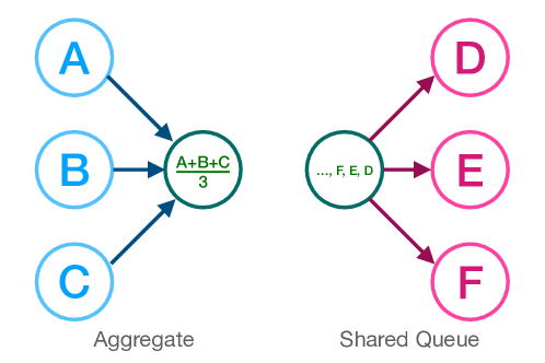
Figure 1. Aggregate and Shared Queue Operators

Before describing how data are communicated, it is worth clarifying the semantics of the task model in EdgeServe EdgeServe has two key distributed operators illustrated in Figure 1: aggregate(delay) and shared_queue(). These are analogous to their non-streaming counterparts (e.g., reduce). These two operators sit between data consumers and producers to ensure that computation is appropriately placed in the network. They can actually be thought of as special “models” in our system whose sole purpose is multiplexing and demultiplexing data streams.

aggregate(delay). Whenever streaming data from multiple nodes need to be combined in order to make a prediction, the aggregate operator is applied. An aggregate operator consumes data from multiple streams and produces a single iterator interface for a data consumer. The operator takes a user-specified delay as a parameter — the longest tolerable time skew between data sources. The operator waits until the skew timeout is met for data from all senders to arrive and yields a combined tuple. This tuple might contain missing values for streams that did not produce data within the time window.

shared_queue(). The shared_queue() operator multiplexes a stream into multiple streams of data, or demultiplexes multiple streams into one stream of data. Nodes can consume data from each individual stream and perform model inferences. After inference, we can also use an aggregate operator to merge the predictions back into a single time-synchronized stream.

4.3. Lazy Data Routing

A message broker system consists of a leader that orchestrates the entire message flow and multiple producers/consumers as message endpoints. Data streams as producers publish data to the leader, and models as consumers consume data from the leader. With this architecture, the leader can quickly become a point of contention since it has to process all the messages from/to all the different nodes. Furthermore, large message payloads (e.g., images) can lead to a crucial networking bottleneck at the leader, as message broker systems are not designed to handle large messages.

EdgeServe uses a novel messaging protocol to efficiently transfer data between nodes without placing an undue burden on the leader. A message sent to the leader only contains message headers: a timestamp and a global source path. The actual message payloads are not transferred; instead, they are kept and indexed on the node that collected the data. A model subscribes to the topic and reads the headers as they come in. If it wants a particular data payload, it retrieves that data lazily from the source node.

Figure 2 illustrates this protocol. When collecting data, every data item added to a DataStream is annotated with a header (Figure 2-1). We can think of this as a stream of $(h,d)$ tuples (header and data, respectively). After the tuple is created, the node locally writes the data to a time-indexed log (Figure 2-2). After this data is durably written, the header is published to the message broker on the leader (Figure 2-3). Nodes on the network can subscribe to streams of these headers. Model inference requires the data payload, and that can be requested from the headers (Figure 2-4). This data is transferred in a peer-to-peer fashion, and inferences happen over these streams (Figure 2-5).

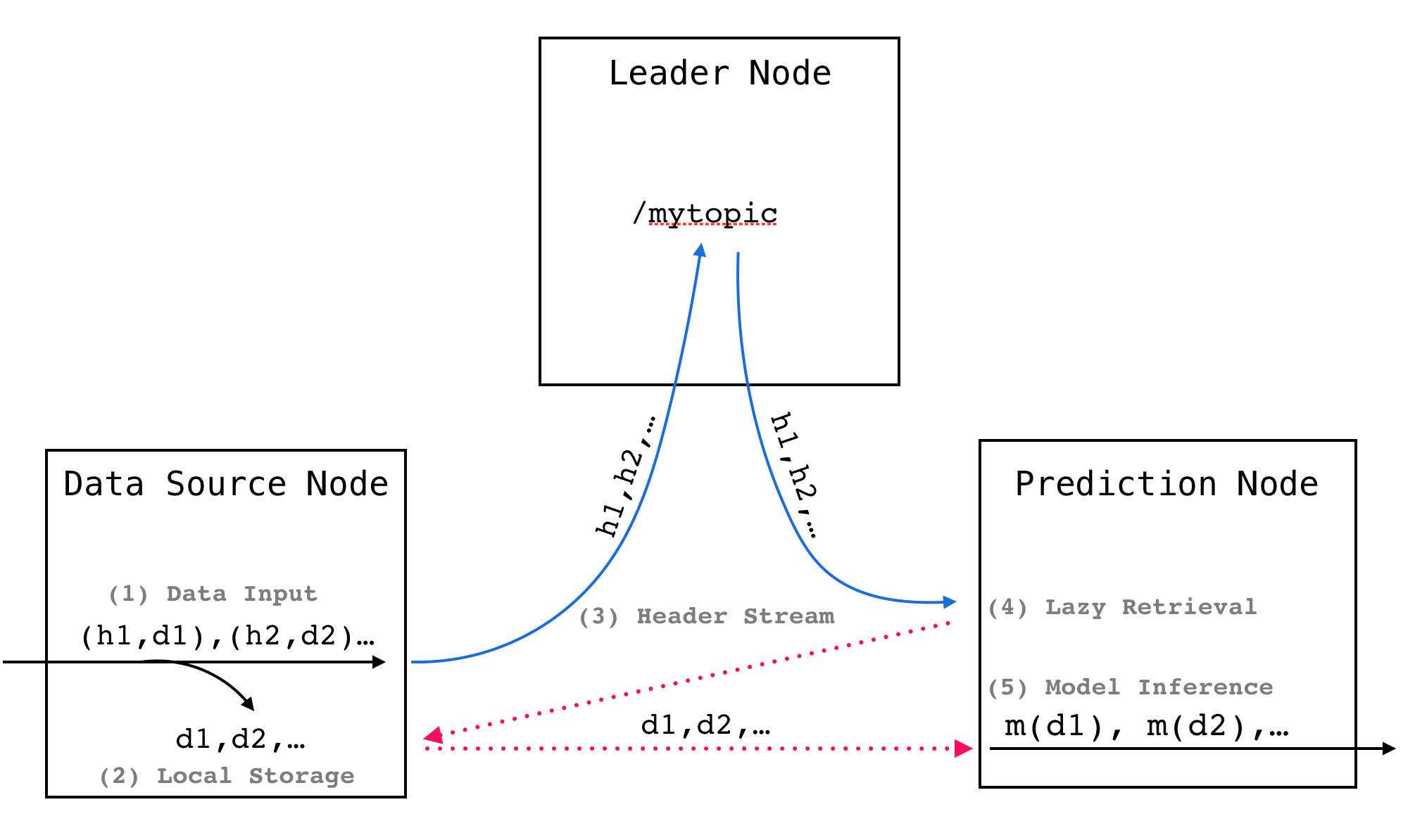
Figure 2. A figure illustrating the order of operations in the lazy data routing system used by EdgeServe.

Lazy retrieval has a number of essential benefits for typical model-serving tasks. In general, these benefits are analogous to that of lazy computation. First, many models predict at rates much slower than the rate of data collection. For example, a model that takes 30ms to evaluate can only process one example every 30ms. If the data collection rate is significantly faster than that, the model often has to downsample the input data. Lazy data routing allows us to avoid transferring the data payload to the leader in these cases. Next, this strategy reduces the size of the messages processed by the message broker reducing overheads in checkpointing and serialization/de-serialization. As a result, we also find that it can enable increased parallelism as well. Both of these benefits can be tied back to the traits of the machine learning setting mentioned above.

4.3.1. Other Considerations

Practically, every edge node has a limited amount of local storage. EdgeServe handles this by having a timeout for the data payloads, where a node on the network can only send a retrieval request within that timeout. This allows the edge node to overwrite/free up that space periodically.

In certain cases, we allow users to force EdgeServe to have eager message passing. Small messages, such as 1D arrays, can be transferred from data source nodes to worker nodes via the leader node. Essentially, this embeds the payload in the message headers. In some networks, peer-to-peer communication is not available or not efficient. We can default to eager message passing when needed to support these cases.

5. Ensuring Prediction Timeliness

Next, we show how to ensure this execution layer can meet particular model-serving SLOs. We leverage statistical approximations that exploit temporal similarity in typical data streams. Every model in EdgeServe is annotated with two timing parameters:

• If it consumes multiple streams, a maximum tolerable skew.

• A target prediction frequency., which is the desired rate of output.

5.1. Message Skew

EdgeServe gives the programmer an illusion of stream alignment, namely, streams associated with the same topic can be thought of as synchronized from the perspective of machine learning modeling. The consuming models receive tuples of headers corresponding to data from each of the sources. Figure 3 shows this point: from a programmer’s perspective, the entire topic can be treated as a single stream.

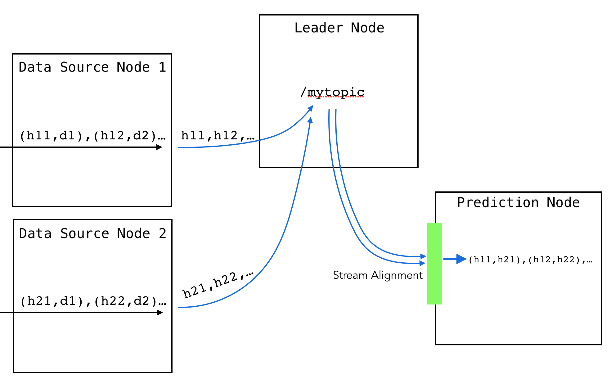
Figure 3. A model subscribes to a single topic which might include multiple streams of data. EdgeServe ensures that multiple streams of data are time-aligned as tuples in order to make predictions.

Under the hood, EdgeServe has to buffer streams locally to keep up this illusion. The different data streams will arrive at different rates and have different systems delays that cause misalignment. We use a time interval-based interface for specifying alignment criteria. Thus, every topic has a maximum allowed time-skew between headers that can be produced. Locally, the buffer retains a header until it receives matching header messages from other sensors. Thus, we can enforce a bounded-skew synchronization on the model side. This heavily depends on a reasonable time interval requested between predictions. If such time interval is too short, such synchronization can be ineffective without improving accuracy; if the time interval is too long, potential long waits can stretch end-to-end timeliness while harming accuracy due to lost high-frequency information in between.

5.2. Target Prediction Frequency

In classical data streaming systems, “back pressure” is a mechanism used to control the rate at which data is processed by the system in order to prevent overload and ensure stability (e.g., as in Apache Flink (Carbone et al., 2015)). Back pressure is usually applied when there is a mismatch between the rate at which data is being produced by the data source and the rate at which it can be processed by the downstream components of the system. In such cases, the system may experience a backlog of data that has yet to be processed, leading to increased latency and decreased throughput.

Similarly, model-serving systems are rate-limited by the decision processes that consume their predictions. This might be a monitoring dashboard subject to visualization refresh rates, or an SLO describing a desired reaction time. In EdgeServe, users can annotate models with a target prediction frequency. This prediction frequency downsamples data if the data arrival rate exceeds what is attainable (i.e., like back-pressure). Conversely, if some data arrive slower than this target frequency, it provides a timeout for how long we have to wait for asynchronous messages.

To see how this works, let’s work with a simple single-model example. Assume the following data stream arrives in the system:

$$(\textsf{time},\text{data})=(1,x_{1}),(3,x_{3}),(4,x_{4}),(6,x_{6})$$

Without a target frequency, the system would yield the following predictions for each arriving example at the corresponding times:

$$(\textsf{time},\text{res})=(1,f(x_{1})),(3,f(x_{3})),(4,f(x_{4})),(6,f(x_{6}))$$

Instead of synchronizing predictions on data arrival, a prediction frequency target synchronizes predictions based on a timer. It yields a prediction from the last known observation at that time. Let us consider the case where a user wants to rate-limit the system. For example, a frequency of $2$ in the example above would yield predictions at (2,4,6). The latest data is always used to produce this prediction.

$$(\textsf{time},\text{res})=(2,f(x_{1})),(4,f(x_{4})),(6,f(x_{6})))$$

As we can see in this example, if the prediction frequency is slower than the data arrival rate, substantial data skipping is possible. It gives us an additional knob to optimize data transfer, where the system need not yield predictions faster than the desired target. For the example above, time-step $3$ is never consumed by the inference node. This means that certain header messages are ignored, and thus lazy data routing saves us from transferring those data payloads. A significant amount of communication can be saved if some data streams arrive faster than the desired prediction frequency. However, there is a natural trade-off of staleness that arises with this approach.

5.3. Tolerating Incomplete Messages

Target frequencies and skews can also be used to tolerate variable or fault-prone data streams. Suppose one sets the target frequency to be at the P95 data arrival rate; it can be used to generate a timeout on the message broker. If new data from one source has not arrived before the timeout, the timer will have to short-circuit with a partial message only containing data from a subset of the sources. Such anomalies can happen if there is a temporary failure on one of the data source nodes, or a large network delay.

In these cases, we do not want the system to fail. EdgeServe provides a number of fail-soft mechanisms to rectify the issue, such as dropping the tuple and imputing the missing values with a last known good observation. In our experiments, we use last-known-good-data as our primary fail-soft strategy. In the example above with a target of $2$, suppose the following stream of data had a failure at example $t=3$:

$$(\textsf{time},\text{data})=(1,f(x_{1})),(3,\blacksquare),(4,f(x_{4})),(6,f(x_{6}))$$

The system would yield the following predictions:

$$(\textsf{time},\text{result})=(2,f(x_{1})),(4,f(x_{4})),(6,f(x_{6}))$$

Now, suppose the target was $1$, the result would be:

$$(\textsf{time},\text{result})=(1,f(x_{1})),(2,f(x_{1})),(3,f(x_{1})),...,(6,f(x_{6}))$$

In dense streams of data, such a strategy leverages temporal correlations where the last known observation is likely similar to the missing data. This allows the prediction stream to fail soft in the presence of jitter and temporary failures.

6. Experiments

We evaluate EdgeServe in both micro-benchmarks and end-to-end experiments.

6.1. Experimental Setup

All of our experiments are performed on a private “edge cluster”. Our hardware setup consists of 5 NVIDIA Jetson Nano Developer Kits and 4 Intel Skylake NUC computers. Each NUC is equipped with an Intel Core i3-6100U CPU, 16 GB memory and M.2 SSD. Throughout these experiments, we vary the network topology to test various scenarios. These variations will be explained in the experiment sections. Generally, NUCs are used as the leader node and 3 data source nodes; Jetson Nanos are used as 1 other data source node and all prediction nodes.

As a primary baseline, we have also configured PyTorch distributed (Li et al., 2020) on our edge cluster, with Gloo as the distributed communication backend. We run PyTorch in both a centralized mode (traditional model serving) as well as a decentralized mode when possible. We have also implemented an architecture similar to ROS (Quigley et al., 2009) within our framework to understand the key design decisions. ROS is widely used in the sensor and robotics communities and provides a centralized message broker service. However, ROS does not support lazy data routing, distributed stream alignment, and adaptive rate control. We excluded Tensorflow from this evaluation because we found that the TensorFlow Distributed did not give us the fine-grained control over communication needed for fair experiments. For synchronization-sensitive experiments, we set up a local NTP server to make sure all nine nodes share a global wall clock time.

6.2. Evaluation Metrics

We borrow the following common metrics used in streaming systems (Karimov et al., 2018) to measure the system performance of EdgeServe.

6.2.1. Types of Latency

Producer Sending Latency. We define producer sending latency to be the interval between the time the producer begins sending an example to the leader node and the time the producer finishes sending the same example to the leader node.

Consumer Receiving Latency. We define consumer receiving latency to be the interval between the time the producer finishes sending an example to the leader node and the time the consumer finishes receiving the same example from the leader node. That means, if there is any queuing backlog at the leader node, it is counted as part of consumer receiving latency.

Total Communication Latency. We define total communication latency to be the sum of producer sending latency and consumer receiving latency. It means the interval between the time the producer begins sending an example to the leader node and the time the consumer finishes receiving the same example from the leader node.

Processing Latency. We define processing latency to be the interval between the time a prediction node starts processing an example (or an aggregated set of examples) and the time it finishes processing the same example. The processing latency is used to measure the actual computation time of an example (or an aggregated set of examples).

End-to-end Latency. We measure the interval between the time an example is collected by EdgeServe and the time the last prediction node finishes processing the same example as end-to-end latency. The end-to-end latency includes but not limited to total communication latency and processing latency.

Total Working Duration. We define total working duration to be the interval between the time the producer begins sending the first example of a task to the leader node and the time the last prediction node finishes processing the last example of the task. This is a task-level measurement rather than a per-example measurement, and it includes both communication time and computation time (if any).

6.2.2. Backlog

We define the end-to-end latency of the last example of a task as backlog. Backlog is an important metric because all kinds of delays can easily accumulate, which causes outdated predictions for later examples in a real-time inference scenario. The lower bound of the backlog is near-zero, when there is no delay along the path from the data source to prediction nodes. Ideally, such lower bound is achievable if data arrive slower than the rate our computational power can serve, or we might have to skip some data points to keep the predictions in time.

6.2.3. Real-time Accuracy.

When it comes to real-time prediction tasks, the timeliness of predictions becomes a key concern of user experience. For latency-sensitive tasks, late prediction is incorrect prediction. To evaluate the timeliness of predictions, we define real-time accuracy to be the accuracy of predictions compared with the last known label at prediction time. For example, suppose a prediction is made temporally between two consecutive labels with timestamps $t_{1}$ and $t_{2}$ ($t_{1}\leq t_{2}$). In that case, we compare the prediction result to the ground truth at $t_{1}$ to calculate the real-time accuracy. Since we assume adjacent examples are likely similar, we expect roughly correct prediction results when the examples arrive slightly late. However, if the examples arrive significantly late, they are likely outdated and yield incorrect predictions.

6.2.4. Excess Examples Processed.

Asynchronous messaging systems like EdgeServe will naturally have to tolerate jitter and unpredictable pattern of message arrivals. Downsampling and upsampling are necessary to meet a prediction frequency target. We evaluate the degree of these effects in terms of excess examples processed. In a synchronous system, a certain number of inferences will be served. Here, we measure how many extra inferences the system upsampled to hit the prediction frequency target. If the number of excess examples processed is less than 0, it means EdgeServe performed downsampling to ensure timely predictions.

6.3. Benefits of Lazy Data Routing

In Section 4, we described our lazy data routing model as an alternative to a ROS-like system that eagerly transfers raw data through a centralized broker. Now, we evaluate the pros and cons of the lazy data routing model.

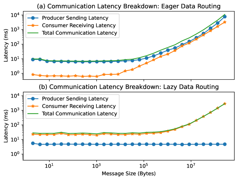
Figure 4. Lazy data routing reduces latency on producer side but has fixed overhead on consumer side. Both axes are log-scaled.

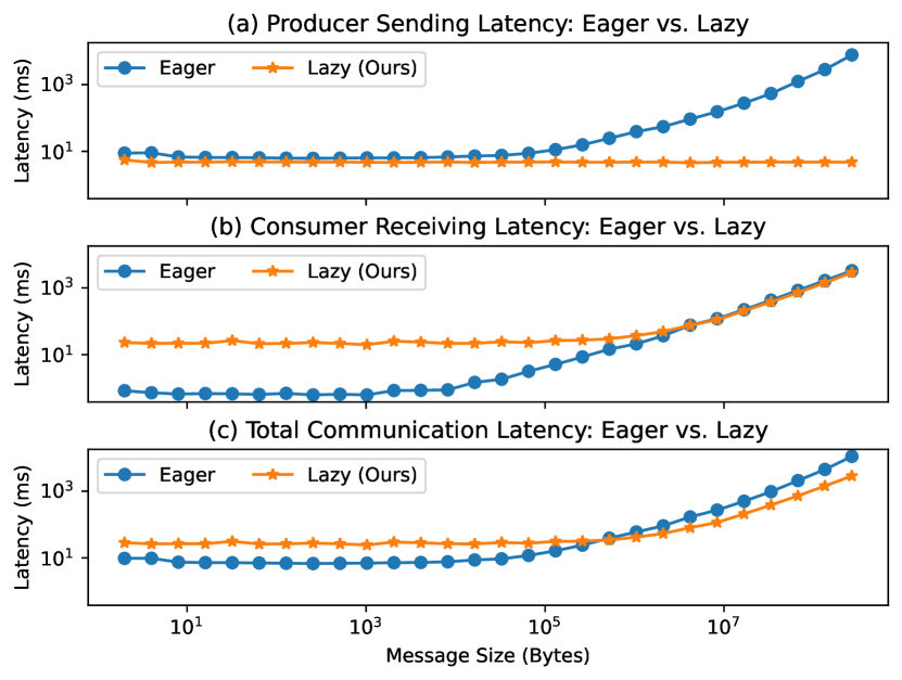
Figure 5. Lazy data routing reduces latency on producer side but has fixed overhead on consumer side. Both axes are log-scaled.

First, we send a series of messages of different sizes from a data source node to a prediction node, through the leader node. No actual computation is performed. We compare the communication latency between eager and lazy data routing.

6.3.1. Lazy Data Routing Reduces Latency on Producer Side

Since we only need to transfer the headers instead of raw data in our lazy data routing model, the latency on producer side remains a negligible number even if the message is huge. As shown in Figure 4a and 5a, a ROS-like eager data routing model could result in very high latency when sending large messages, which itself could force subsequent messages to queue up and become outdated when they arrive. In contrast, our lazy data routing model makes sure that message headers are sent in milliseconds, which never blocks the rest of messages. The consumers may choose to downsample some data, and only fetch necessary data in a separate process.

6.3.2. Lazy Data Routing Has Fixed Overhead on Consumer Side

Whenever the consumer needs to fetch raw data, there is a fixed overhead to establish P2P connections even if the actual data is just a few bytes. This fixed overhead can be amortized when the actual data is larger, as depicted in Figure 4b and 5b.

6.3.3. Break-Even Point Between Lazy and Eager Data Routing

As a summary of Section 6.3.1 and 6.3.2, lazy data routing is more performant when the messages transferred are larger in size. As shown in Figure 5c, eager data routing actually has a lower total communication latency when the messages are smaller than 512KB in size, and lazy data routing performs better when the messages are larger than 512KB in size.

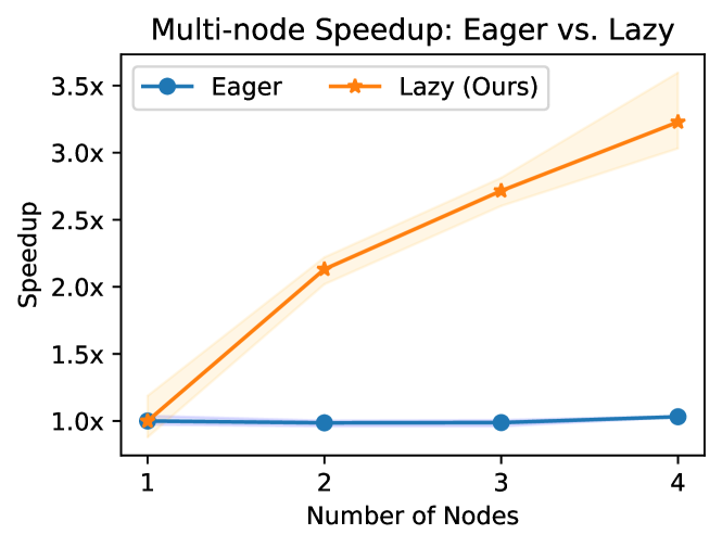
Figure 6. Lazy data routing scales out well while eager data routing does not.

6.3.4. Lazy Data Routing Naturally Supports Parallelism

It is very common for multiple consumers to fetch data from one or more producers at the same time. In our lazy data routing model, since messages are transferred in a peer-to-peer fashion, the leader node only has a very light workload to process tiny headers simultaneously, saving precious bandwidth at the leader node. However, in the eager data routing model, the leader node can be blocked when a piece of large message is going through the leader node from a producer to a consumer. As a result, other producers and/or consumers running in parallel cannot send or receive messages at the same time.

To compare the scalability of communication between eager and lazy data routing models, we have one producer continuously sending the same 512KB message for a total of 100 times to a shared queue. We gradually increase the number of consumer nodes from 1 to 4 and see how it scales out. While no actual computation is done, we measure the total working duration and use the single-node setup for both the eager and lazy data routing as the 1.0x baseline. Figure 6 shows how the eager data routing model fails to scale out with more consumer nodes, while our lazy data routing model achieves reasonable speedup. The line shadows represent the lower and upper bounds of repeated experiments.

6.3.5. Lazy Data Routing Performs Better with Network Contention

Our lazy data routing model is especially beneficial when the leader node is busy with network requests. We specifically construct a task where the message payload is large: real-time inference over video streams. In this experiment, two webcams capture the same moving QR code from different positions. Both videos are 150 frames long at 1920x1080 resolution. Each camera is connected to a unique data source node on the network. For multi-camera tracking, the QR code has to be detected in both streams and corresponded in time-aligned frames from both cameras. So these two data streams need to be aggregated at the prediction node. We simulate a congestion scenario where the network bandwidth at the leader node is limited. Note that the rest of the network retains its full speed; the only congestion is at the leader node.

Table 1 shows the results. With no congestion, the system can process roughly 0.8 frames per second in both lazy and eager data routing. With congestion, the story is very different. Our lazy data routing is tolerant, while transferring raw frames in a ROS-style eager communication pattern can be extremely slow when the network is congested. The total working duration increases by a factor 7 simply due to congestion. Without care, distributed, multi-sensor deployments can easily lose real-time processing capabilities if the broker becomes a point of contention. These experiments illustrate the value of EdgeServe in a controlled scenario, where we can isolate performance differences.

	Rate limit (up/down)	Time
Lazy (ours)	No limit	3m 10s
Lazy (ours)	1 Mbps / 1 Mbps	3m 12s
Eager (similar to ROS)	No limit	3m 16s
Eager (similar to ROS)	20 Mbps / 20 Mbps	21m 32s

Table 1. Total working duration with network bandwidth limits.

6.3.6. Lazy Data Routing performs better with Data Skipping

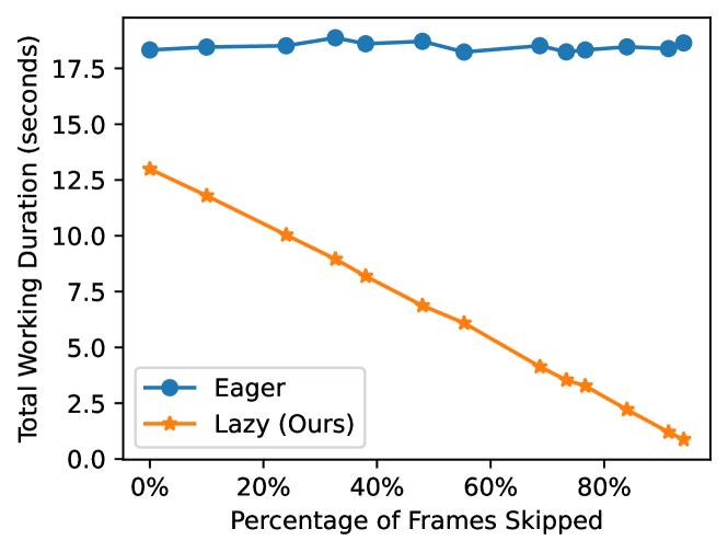
Figure 7. Lazy data routing saves a lot of time in data communication when some data is skipped.

Apart from network congestion, lazy data routing is also valuable when data skipping is employed to ensure the timeliness of prediction results. We take one of the two 150-frame videos mentioned in Section 6.3.5 and transfer these frames from one node to another, via the leader node. Each frame is about 6 MB in its uncompressed form. No actual computation is performed as we are only interested in the communication cost. In Figure 7, we illustrate how much communication cost can be saved by lazy data routing. On the x-axis, we have variable percentage of frames skipped due to adaptive rate control described in Section 5; on the y-axis, we measure the total working duration defined in Section 6.2.1. Even when no frames are skipped, our lazy data routing model performs better than the eager data routing model due to eliminated overhead of transferring a large amount of data through the leader node. When more frames are skipped, our lazy data routing saves communication time almost linearly to the number of frames skipped by the downstream node. On the other hand, the ROS-style eager routing pattern spends roughly the same time on communication even if most of the frames are skipped by the downstream prediction node, because it would transfer the entire data payload upfront anyway.

6.4. Human Activity Recognition

Now, we use the Opportunity dataset for human activity recognition (Roggen et al., 2010; Chavarriaga et al., 2013) as an example to demonstrate the end-to-end performance of EdgeServe in a latency-sensitive scenario. Data from multiple motion sensors were collected about every 33ms while users were executing typical daily activities. For each subject, there are five activity of daily living (ADL) runs, and each run lasts 15-30 minutes. We take the first subject’s first four ADL runs as the training set and the last ADL run as the test set. When played at 2x speed, the last ADL run takes 8 minutes and 22 seconds. We use the first 134 columns and partition these columns vertically into four disjoint subsets, as if they come from different data source nodes: 1-37 (accelerometers), 38-76 (IMU back and right arm), 77-102 (IMU left arm), and 103-134 (IMU shoes). Data from multiple data source nodes need to be combined in order to make a prediction. We train an aggregated random forest model with scikit-learn (Pedregosa et al., 2011) for all 134 features, and also four separate random forest models for each subset of features to evaluate an ensemble method. For the inference stage, we simulate the generation of data at 2x the original speed. In this experiment, we evaluate three ways the task can possibly be done: (Centralized, topology 1) transfer the entire dataset from data source nodes to the destination node, which also acts as the prediction node and does all computations in a centralized way; (Parallel, topology 2) transfer incoming data to a shared queue where four prediction nodes can pull data from when they become available; (Decentralized, topology 3) make predictions locally at data source nodes and only transfer local predictions to the destination node, which then combines local predictions by a majority vote. In our best-effort PyTorch implementation, we use the gather() API to aggregate data from multiple data source nodes. PyTorch distributed requires all tensors to be the same size to be gathered, so we have to pad each local tensor to the maximum size with zeros. Since there is no message queue in PyTorch, it is not possible to compare the parallel (topology 2) strategy between EdgeServe and PyTorch. However, we can still compare centralized and decentralized strategies across these two frameworks.

In this experiment, the individual streams are fast enough that misalignments can occur due to queuing delays. However, PyTorch enforces that multiple data sources are always perfectly synchronized, as we do not begin actual computation until data from all data sources has been gathered, and we only gather new data after finishing previous data items. Such strict requirement does not exist in EdgeServe, as we set a reasonable time interval that allows us to tolerate some amount of skew in examples.

6.4.1. EdgeServe Reduces Serving Backlog.

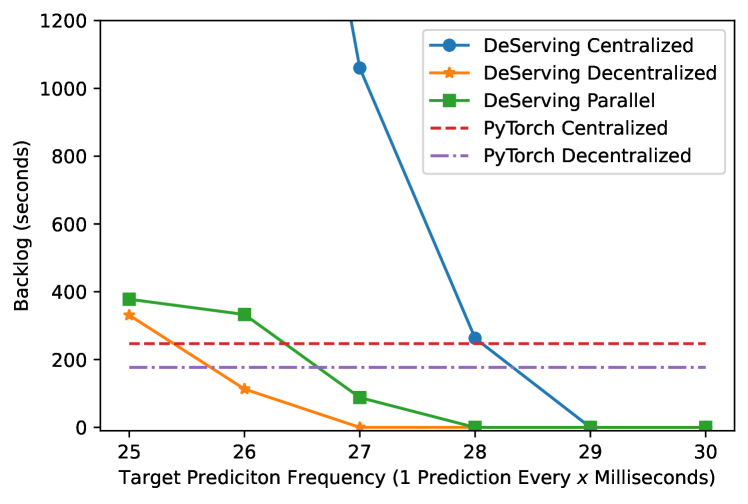
Figure 8. Measure of backlog in the activity recognition task. Higher target frequencies are on the left side and lower frequencies are on the right side. Without proper rate control, a long queue of unprocessed examples is quickly developed.

First, we evaluate the backlog as defined in Section 6.2.2, and the results are shown in Figure 8. The x-axis is the target prediction frequency designated by the end-user, where a larger number means a lower frequency; the y-axis is the backlog for each of the serving systems over this dataset. The compute part of the task itself takes about 23ms to complete, and a near-zero number in backlog means the inference is processed in real time. When target prediction frequency $\geq 29$ms per prediction, all model placements have near-zero backlog. However, if there are a lot of examples yet to be processed, the last example would have to wait in line for a long time (e.g. when target prediction frequency $\leq 26$ms per prediction). Since PyTorch does not offer a message queue and target frequency control, it has to process every single example one by one and aggregates data in a synchronous manner. EdgeServe decentralized offers a no-backlog queue for a wider range of prediction frequency targets ($\geq 27$ms/pred). For both EdgeServe and PyTorch, we see a lower backlog for decentralized model placements because we are able to make the most of local data source nodes and save communication costs. EdgeServe parallel helps reduce the backlog over centralized when the task is compute-bound, for example, when the target prediction frequency is too frequent ($\leq 27$ms/pred). However, this speedup in latency is limited once compute is no longer the bottleneck ($\geq 28$ms/pred).

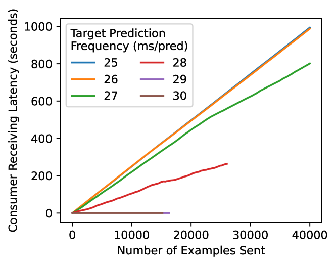
Figure 9. Consumer receiving latency per example for EdgeServe centralized. The queue grows significantly faster when the user requests a higher prediction frequency target (smaller number of ms/pred).

Figure 9 gives us a closer look into the queuing delay. The x-axis is the sequence number of examples sent and the y-axis is the consumer receiving latency of that specific example. Only the first 40000 examples are shown due to brevity. EdgeServe centralized is the model placement strategy used in this experiment. An increasing line means a longer time to wait for later examples to be processed, due to the growing queue. Figure 9 corresponds to Figure 8 that EdgeServe centralized has near-zero backlog when target prediction frequency $\geq 29$ms per prediction.

6.4.2. Decentralized Models Are More Accurate

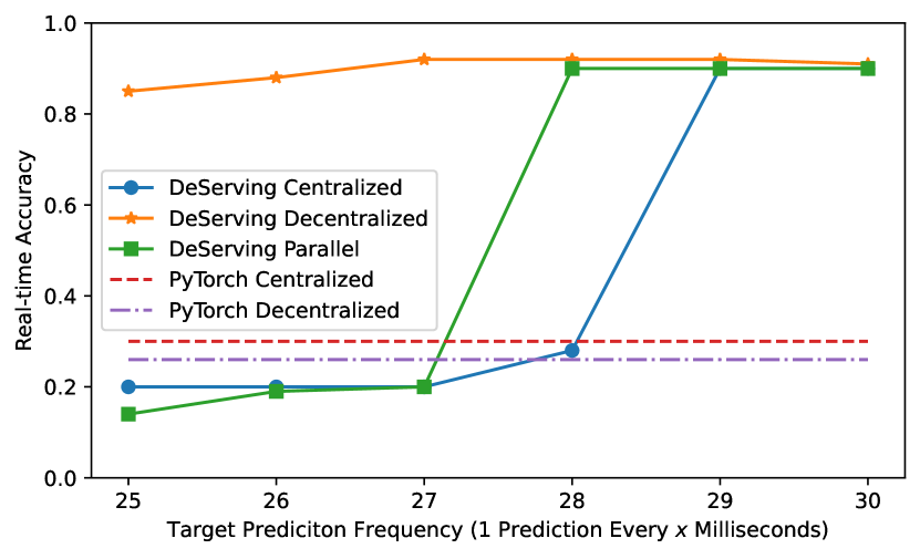
Figure 10. Overall real-time accuracy for human activity recognition task measured in F-1 score. Higher target frequencies are on the left side and lower frequencies are on the right side.

Previous set of experiments show that decentralized models offer a wider operational range of serving in real time. Next, we show that these models can also be substantially more accurate because they offer more timely predictions. Figure 10 shows the real-time accuracy (as defined in Section 6.2.3) of EdgeServe and PyTorch across different model placement strategies and target prediction frequencies. PyTorch distributed is not able to issue accurate predictions because data is communicated in a synchronous manner and it does not downsample the input stream even if the node is overloaded, making most of its predictions outdated. On the other hand, even though messages processed by EdgeServe might not be perfectly aligned temporally, EdgeServe issues much more accurate predictions when the target prediction frequency is infrequent enough for the prediction node(s) to make predictions immediately after new data comes in. For EdgeServe decentralized, the real-time accuracy is still desirable even when the user requests very frequent outputs. There are several reasons behind this. First, local models are usually smaller and takes a shorter time to run. This enables EdgeServe to downsample more incoming data at a certain prediction frequency, so the local models can catch up with data arrival rate better than in a centralized mode. Second, the heterogeneous nature of local data source nodes also plays a role. In our experiment, some data source nodes have better computational power than others and are able to finish local computations faster. When a maximum tolerable skew has passed after the early nodes completed their local work, the ensemble method stops aggregating over all local predictions due to missing data, and thus stops issuing outdated predictions.

6.4.3. Decentralized Models Are More Tolerant to Delays

Real-time accuracy (F-1 score)	No delay	25ms delay
EdgeServe Centralized	0.90	0.55
EdgeServe Parallel	0.90	0.55
EdgeServe Decentralized	0.91	0.85

Table 2. Real-time accuracy measured in F-1 score when one of the four data streams has a constant delay. Decentralized models are more accurate even if there is a delay from one data source.

In this experiment, we assume all architectures achieve a sustainable throughput by setting the target prediction frequency to 30ms/prediction. We evaluate the real-time accuracy of predictions when one of the four data streams have a constant 25ms delay. Table 2 shows that, while parallel and centralized models suffer from considerable degradation in accuracy due to the delay, decentralized models achieves a much higher accuracy even if there is a constant delay. This is because local predictions from other data streams are unaffected and the “unpopular vote” – local prediction of the delayed data stream is likely dropped by the ensemble method.

6.4.4. Decentralized Models Reduce Excess Work.

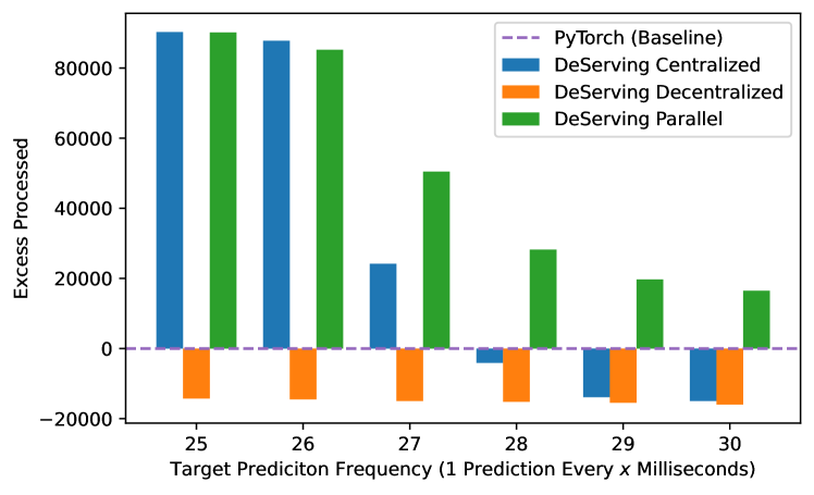
Figure 11. Number of excess examples processed for different strategies and target prediction frequencies. Higher target frequencies are on the left side and lower frequencies are on the right side.

Now, we look at the number of excess examples that are processed to better understand how EdgeServe automatically upsamples/downsamples the incoming data stream to match the rate of prediction. As can be seen from Figure 11, PyTorch (either centralized or decentralized), as a baseline, is marked as zero on the y-axis because it always processes a fixed number of examples equal to the input size. In both centralized and parallel settings, EdgeServe is very sensitive to target prediction frequency because it no longer has to upsample (or even downsample) the incoming data stream when such target is relaxed. Therefore, we see a rapidly decreasing excess work from left to right as the target prediction frequency becomes less frequent. On the other hand, in a decentralized setting, EdgeServe is not as sensitive to such change in target prediction frequency for the same reason why EdgeServe decentralized maintains a high real-time accuracy discussed in Section 6.4.2. The highest target frequency of 25ms/pred is already longer than the typical compute time of a local model on faster local nodes, so some downsampling is performed even at the highest frequency. After faster nodes finish local predictions in almost real-time, the ensemble method simply skips further local predictions made by slower nodes because they are too far behind the last known message sent by each faster node. As a result, decentralized models only process a small number of examples, even when the target prediction frequency is high enough.

Figure 12. Standard deviation of actual prediction frequency for decentralized model placement. Higher target frequencies are on the left side and lower frequencies are on the right side. EdgeServe maintains a lower variability in actual prediction frequencies.

6.4.5. EdgeServe Issues Prediction Results More Stably.

Lastly, we look at the variability in actual prediction frequencies in decentralized settings between EdgeServe and PyTorch. In figure 12, we see a much higher variability in actual prediction frequencies for PyTorch than EdgeServe across all user-defined rates. This is because PyTorch communicates in a synchronous fashion, and has to account for the variability of all 4 nodes making local predictions with local data streams. For EdgeServe, since our data routing is asynchronous, the variability of EdgeServe mostly comes from the imputations of the last known observation and the downsampling of incoming data streams. This variability continues to exist as long as the data arrivals are unpredictable.

6.5. EdgeServe Enables New Serving Topologies

EdgeServe natively allows multiple producers and multiple consumers to operate on the shared message queue at the same time, which is an essential communication paradigm in decentralized prediction but not currently supported by PyTorch or TensorFlow. In this experiment, we show the benefits and overheads of routing data with a shared queue, without further optimizations such as backpressure. Unlike the human activity recognition example in Section 6.4, we are not interested in time-synchronization in this experiment. So we choose a pre-aggregated non-streaming workload that maximizes throughput as its goal.

Network intrusion detection systems (NIDS) monitor network traffic and detect malicious activity by identifying suspicious patterns in incoming packets. Consider an NIDS monitoring traffic in an organization’s private cloud. On different nodes in this network, there are network packet captures that are tracking that node’s incoming and outgoing network traffic. All of this data is aggregated into a set of features that are fed into a predictive model that predicts whether the system is under attack or not.

We use a public Network Intrusion Detection dataset from Canadian Institute for Cybersecurity (CIC-IDS2017) (Sharafaldin et al., 2018) and an existing model to differentiate malicious traffic from benign network traffic (Kostas, 2018). Specifically, we partition the data horizontally into four disjoint subsets by “Source IP” for our four data source nodes. The underlying assumption is that network traffic from different source IP addresses may be collected separately.

If a web attack is detected, the related network packet needs to be sent to a specific destination node, but the actual computation can be done anywhere. Similar to the three topologies in Section 6.4, we can choose from the following three strategies: (Centralized, topology 1) transfer all data to the prediction node that does all computations in a centralized way; (Parallel, topology 2) transfer all data from data source nodes to an intermediate shared queue, where four prediction nodes can pull data from when they become available, and they need to inform the destination node if an attack is detected; or (Decentralized, topology 3) data source nodes do computations locally and only transfer data to the destination node if an attack is detected.

In our best-effort PyTorch implementation, we use send() and recv() APIs to communicate between nodes, where data source nodes send data to the destination node, and the destination node receives data from all other nodes. However, to the best of our knowledge, there does not exist an API in the current PyTorch distributed framework where we can send/receive data to/from a shared queue, so Parallel (topology 2) strategy can only be implemented in EdgeServe.

In a centralized setting, PyTorch distributed is able to process 41.94 examples per second, while EdgeServe can process 47.58 examples per second. This is the baseline setting of both systems, and the performances of both systems are comparable. In a Parallel setting that is only supported by EdgeServe thanks to its queuing design, 182.57 examples are processed per second, which is almost a linear (3.84x) speedup compared to a centralized setting given that we now have 4 prediction nodes. In a decentralized setting, we make all 4 data source nodes also local prediction nodes, and PyTorch achieves 181.33 examples per second while EdgeServe takes 197.30 examples per second. For both systems, superlinear speedup (4.32x and 4.15x compared to centralized, respectively) is achieved by making the most of local computational resources and communicating only local prediction results instead of the entire dataset. Since we use the same model/sub-models for both EdgeServe and PyTorch without synchronization issues, the accuracies of predictions between both systems are the same.

In short, the results of this experiment can be summarized as follows: (1) the baseline performance of EdgeServe is at least comparable to PyTorch, (2) EdgeServe offers a wider range of decentralized prediction topologies, and (3) decentralized prediction can significantly improve overall prediction performance for both PyTorch and EdgeServe.

7. Conclusion

There is a lot of community interest in distributed and federated problems in machine learning (Konečný et al., 2015). We believe that the inference setting is under-studied despite a clear need in a number of different domains. This paper focuses its discussion on the execution layer for decentralized prediction systems. The paper contributes the communication primitives needed to make such systems work in practice. We find that decentralized prediction can give system designers new knobs to enable real-time predictions. Our results show: (1) a clear value for decentralization, (2) that EdgeServe is an effective architecture for supporting decentralization, and (3) core techniques in EdgeServe, such as lazy data routing, are broadly applicable to modern stream processing.

References

- (1)
- Abadi et al. (2016) Martín Abadi, Paul Barham, Jianmin Chen, Zhifeng Chen, Andy Davis, Jeffrey Dean, Matthieu Devin, Sanjay Ghemawat, Geoffrey Irving, Michael Isard, Manjunath Kudlur, Josh Levenberg, Rajat Monga, Sherry Moore, Derek G. Murray, Benoit Steiner, Paul Tucker, Vijay Vasudevan, Pete Warden, Martin Wicke, Yuan Yu, and Xiaoqiang Zheng. 2016. TensorFlow: A System for Large-scale Machine Learning. In Proceedings of the 12th USENIX Conference on Operating Systems Design and Implementation (Savannah, GA, USA) (OSDI’16). USENIX Association, Berkeley, CA, USA, 265–283. http://dl.acm.org/citation.cfm?id=3026877.3026899
- Alphabet Inc. (2022) Alphabet Inc. 2022. Tensorflow Case Studies. https://www.tensorflow.org/about/case-studies (visited on October 5, 2022).
- Apache (2022) Apache. 2022. Apache Pulsar. https://pulsar.apache.org/ (visited on March 27, 2022).
- Arulraj (2022) Joy Arulraj. 2022. Accelerating Video Analytics. ACM SIGMOD Record 50, 4 (2022), 39–40.
- Bonawitz et al. (2019) Keith Bonawitz, Hubert Eichner, Wolfgang Grieskamp, Dzmitry Huba, Alex Ingerman, Vladimir Ivanov, Chloé Kiddon, Jakub Konečný, Stefano Mazzocchi, Brendan McMahan, Timon Van Overveldt, David Petrou, Daniel Ramage, and Jason Roselander. 2019. Towards Federated Learning at Scale: System Design. In Proceedings of Machine Learning and Systems, A. Talwalkar, V. Smith, and M. Zaharia (Eds.), Vol. 1. 374–388. https://proceedings.mlsys.org/paper/2019/file/bd686fd640be98efaae0091fa301e613-Paper.pdf
- Carbone et al. (2015) Paris Carbone, Asterios Katsifodimos, Stephan Ewen, Volker Markl, Seif Haridi, and Kostas Tzoumas. 2015. Apache flink: Stream and batch processing in a single engine. The Bulletin of the Technical Committee on Data Engineering 38, 4 (2015).
- Chandrasekaran and Franklin (2003) Sirish Chandrasekaran and Michael J Franklin. 2003. PSoup: a system for streaming queries over streaming data. The VLDB Journal 12, 2 (2003), 140–156.
- Chavarriaga et al. (2013) Ricardo Chavarriaga, Hesam Sagha, Alberto Calatroni, Sundara Tejaswi Digumarti, Gerhard Tröster, José del R. Millán, and Daniel Roggen. 2013. The Opportunity challenge: A benchmark database for on-body sensor-based activity recognition. Pattern Recognition Letters 34, 15 (2013), 2033–2042. https://doi.org/10.1016/j.patrec.2012.12.014 Smart Approaches for Human Action Recognition.
- Crankshaw et al. (2020) Daniel Crankshaw, Gur-Eyal Sela, Xiangxi Mo, Corey Zumar, Ion Stoica, Joseph Gonzalez, and Alexey Tumanov. 2020. InferLine: latency-aware provisioning and scaling for prediction serving pipelines. In SoCC ’20: ACM Symposium on Cloud Computing, Virtual Event, USA, October 19-21, 2020, Rodrigo Fonseca, Christina Delimitrou, and Beng Chin Ooi (Eds.). ACM, 477–491. https://doi.org/10.1145/3419111.3421285
- Crankshaw et al. (2017) Daniel Crankshaw, Xin Wang, Giulio Zhou, Michael J. Franklin, Joseph E. Gonzalez, and Ion Stoica. 2017. Clipper: A Low-Latency Online Prediction Serving System. In 14th USENIX Symposium on Networked Systems Design and Implementation, NSDI 2017, Boston, MA, USA, March 27-29, 2017, Aditya Akella and Jon Howell (Eds.). USENIX Association, 613–627. https://www.usenix.org/conference/nsdi17/technical-sessions/presentation/crankshaw
- Eigen et al. (2013) David Eigen, Marc’Aurelio Ranzato, and Ilya Sutskever. 2013. Learning factored representations in a deep mixture of experts. arXiv preprint arXiv:1312.4314 (2013).
- Flink (2022) Apache Flink. 2022. FlinkML Documentation. https://nightlies.apache.org/flink/flink-ml-docs-master/ (visited on October 5, 2022).
- Han et al. (2016) Song Han, Huizi Mao, and William J. Dally. 2016. Deep Compression: Compressing Deep Neural Network with Pruning, Trained Quantization and Huffman Coding. In 4th International Conference on Learning Representations, ICLR 2016, San Juan, Puerto Rico, May 2-4, 2016, Conference Track Proceedings.
- Horchidan et al. (2022) Sonia Horchidan, Emmanouil Kritharakis, Vasiliki Kalavri, and Paris Carbone. 2022. Evaluating model serving strategies over streaming data. In Proceedings of the Sixth Workshop on Data Management for End-To-End Machine Learning. 1–5.
- Hung et al. (2018) Chien-Chun Hung, Ganesh Ananthanarayanan, Peter Bodik, Leana Golubchik, Minlan Yu, Paramvir Bahl, and Matthai Philipose. 2018. Videoedge: Processing camera streams using hierarchical clusters. In 2018 IEEE/ACM Symposium on Edge Computing (SEC). IEEE, 115–131.
- Kang et al. (2017) Daniel Kang, John Emmons, Firas Abuzaid, Peter Bailis, and Matei Zaharia. 2017. NoScope: optimizing neural network queries over video at scale. Proceedings of the VLDB Endowment 10, 11 (2017), 1586–1597.
- Karimov et al. (2018) Jeyhun Karimov, Tilmann Rabl, Asterios Katsifodimos, Roman Samarev, Henri Heiskanen, and Volker Markl. 2018. Benchmarking Distributed Stream Data Processing Systems. In 34th IEEE International Conference on Data Engineering, ICDE 2018, Paris, France, April 16-19, 2018. IEEE Computer Society, 1507–1518. https://doi.org/10.1109/ICDE.2018.00169
- Konečný et al. (2015) Jakub Konečný, Brendan McMahan, and Daniel Ramage. 2015. Federated Optimization: Distributed Optimization Beyond the Datacenter. CoRR abs/1511.03575 (2015). arXiv:1511.03575 http://arxiv.org/abs/1511.03575
- Kostas (2018) Kahraman Kostas. 2018. Anomaly Detection in Networks Using Machine Learning. Master’s thesis. University of Essex, Colchester, UK.
- Li et al. (2020) Shen Li, Yanli Zhao, Rohan Varma, Omkar Salpekar, Pieter Noordhuis, Teng Li, Adam Paszke, Jeff Smith, Brian Vaughan, Pritam Damania, and Soumith Chintala. 2020. PyTorch Distributed: Experiences on Accelerating Data Parallel Training. Proc. VLDB Endow. 13, 12 (2020), 3005–3018. https://doi.org/10.14778/3415478.3415530
- Liu et al. (2023) Shinan Liu, Tarun Mangla, Ted Shaowang, Jinjin Zhao, John Paparrizos, Sanjay Krishnan, and Nick Feamster. 2023. AMIR: Active Multimodal Interaction Recognition from Video and Network Traffic in Connected Environments. Proc. ACM Interact. Mob. Wearable Ubiquitous Technol. 7, 1, Article 21 (mar 2023). https://doi.org/10.1145/3580818
- Maheshwari et al. (2019) Sumit Maheshwari, Wuyang Zhang, Ivan Seskar, Yanyong Zhang, and Dipankar Raychaudhuri. 2019. EdgeDrive: Supporting advanced driver assistance systems using mobile edge clouds networks. In IEEE INFOCOM 2019-IEEE Conference on Computer Communications Workshops (INFOCOM WKSHPS). IEEE, 1–6.
- Malpani et al. (2000) Navneet Malpani, Jennifer L Welch, and Nitin Vaidya. 2000. Leader election algorithms for mobile ad hoc networks. In Proceedings of the 4th international workshop on Discrete algorithms and methods for mobile computing and communications. 96–103.
- Moritz et al. (2018) Philipp Moritz, Robert Nishihara, Stephanie Wang, Alexey Tumanov, Richard Liaw, Eric Liang, Melih Elibol, Zongheng Yang, William Paul, Michael I Jordan, et al. 2018. Ray: A distributed framework for emerging AI applications. In 13th USENIX Symposium on Operating Systems Design and Implementation (OSDI 18). 561–577.
- Narayanan et al. (2019) Deepak Narayanan, Aaron Harlap, Amar Phanishayee, Vivek Seshadri, Nikhil R Devanur, Gregory R Ganger, Phillip B Gibbons, and Matei Zaharia. 2019. PipeDream: generalized pipeline parallelism for DNN training. In Proceedings of the 27th ACM Symposium on Operating Systems Principles. 1–15.
- Olston et al. (2017) Christopher Olston, Fangwei Li, Jeremiah Harmsen, Jordan Soyke, Kiril Gorovoy, Li Lao, Noah Fiedel, Sukriti Ramesh, and Vinu Rajashekhar. 2017. TensorFlow-Serving: Flexible, High-Performance ML Serving. In Workshop on ML Systems at NIPS 2017.
- Pedregosa et al. (2011) F. Pedregosa, G. Varoquaux, A. Gramfort, V. Michel, B. Thirion, O. Grisel, M. Blondel, P. Prettenhofer, R. Weiss, V. Dubourg, J. Vanderplas, A. Passos, D. Cournapeau, M. Brucher, M. Perrot, and E. Duchesnay. 2011. Scikit-learn: Machine Learning in Python. Journal of Machine Learning Research 12 (2011), 2825–2830.
- Quigley et al. (2009) Morgan Quigley, Ken Conley, Brian Gerkey, Josh Faust, Tully Foote, Jeremy Leibs, Rob Wheeler, Andrew Y Ng, et al. 2009. ROS: an open-source Robot Operating System. In ICRA workshop on open source software, Vol. 3. Kobe, Japan, 5.
- Rocklin (2015) Matthew Rocklin. 2015. Dask: Parallel computation with blocked algorithms and task scheduling. In Proceedings of the 14th python in science conference, Vol. 130. Citeseer, 136.
- Roggen et al. (2010) Daniel Roggen, Alberto Calatroni, Mirco Rossi, Thomas Holleczek, Kilian Förster, Gerhard Tröster, Paul Lukowicz, David Bannach, Gerald Pirkl, Alois Ferscha, Jakob Doppler, Clemens Holzmann, Marc Kurz, Gerald Holl, Ricardo Chavarriaga, Hesam Sagha, Hamidreza Bayati, Marco Creatura, and José del R. Millàn. 2010. Collecting complex activity datasets in highly rich networked sensor environments. In 2010 Seventh International Conference on Networked Sensing Systems (INSS). 233–240. https://doi.org/10.1109/INSS.2010.5573462
- Sagi and Rokach (2018) Omer Sagi and Lior Rokach. 2018. Ensemble learning: A survey. Wiley Interdisciplinary Reviews: Data Mining and Knowledge Discovery 8, 4 (2018), e1249.
- Shaowang et al. (2021) Ted Shaowang, Nilesh Jain, Dennis D Matthews, and Sanjay Krishnan. 2021. Declarative data serving: the future of machine learning inference on the edge. Proceedings of the VLDB Endowment 14, 11 (2021), 2555–2562.
- Shaowang et al. (2022) Ted Shaowang, Xi Liang, and Sanjay Krishnan. 2022. Sensor Fusion on the Edge: Initial Experiments in the EdgeServe System. In Proceedings of The International Workshop on Big Data in Emergent Distributed Environments (Philadelphia, Pennsylvania) (BiDEDE ’22). Association for Computing Machinery, New York, NY, USA, Article 8, 7 pages. https://doi.org/10.1145/3530050.3532924
- Sharafaldin et al. (2018) Iman Sharafaldin, Arash Habibi Lashkari, and Ali A. Ghorbani. 2018. Toward Generating a New Intrusion Detection Dataset and Intrusion Traffic Characterization. In Proceedings of the 4th International Conference on Information Systems Security and Privacy, ICISSP 2018, Funchal, Madeira - Portugal, January 22-24, 2018, Paolo Mori, Steven Furnell, and Olivier Camp (Eds.). SciTePress, 108–116. https://doi.org/10.5220/0006639801080116
- Tensorflow (2022) Tensorflow. 2022. Robust machine learning on streaming data using Kafka and Tensorflow-IO. https://www.tensorflow.org/io/tutorials/kafka (visited on October 5, 2022).
- Zeng et al. (2020) Xiao Zeng, Biyi Fang, Haichen Shen, and Mi Zhang. 2020. Distream: scaling live video analytics with workload-adaptive distributed edge intelligence. In Proceedings of the 18th Conference on Embedded Networked Sensor Systems. 409–421.
- Zhao et al. (2023) Yucheng Zhao, Chong Luo, Chuanxin Tang, Dongdong Chen, Noel Codella, and Zheng-Jun Zha. 2023. Streaming Video Model. In Proceedings of the IEEE/CVF Conference on Computer Vision and Pattern Recognition. 14602–14612.
- Zhuang et al. (2021) Siyuan Zhuang, Zhuohan Li, Danyang Zhuo, Stephanie Wang, Eric Liang, Robert Nishihara, Philipp Moritz, and Ion Stoica. 2021. Hoplite: efficient and fault-tolerant collective communication for task-based distributed systems. In Proceedings of the 2021 ACM SIGCOMM 2021 Conference. 641–656.