OptBA: Optimizing Hyperparameters with the Bees Algorithm for Improved Medical Text Classification

Abstract

One of the challenges that artificial intelligence engineers face, specifically in the field of deep learning is obtaining the optimal model hyperparameters. The search for optimal hyperparameters usually hinders the progress of solutions to real-world problems such as healthcare. To overcome this hurdle, the proposed work introduces a novel mechanism called “OptBA” to automatically fine-tune the hyperparameters of deep learning models by leveraging the Bees Algorithm, which is a recent promising swarm intelligence algorithm. In this paper, the optimization problem of OptBA is to maximize the accuracy in classifying ailments using medical text, where initial hyperparameters are iteratively adjusted by specific criteria. Experimental results demonstrate a noteworthy enhancement in accuracy with approximately 1.4%. This outcome highlights the effectiveness of the proposed mechanism in addressing the critical issue of hyperparameter optimization and its potential impact on advancing solutions for healthcare and other societal challenges.

Introduction

In the recent past, the expansion of the COVID-19 pandemic has reshaped the world radically. Hospitals and medical centers have become fertile ground for the spread of this virus. Social distancing plays a pivotal role in eliminating the spread of this virus (Lotfi, Hamblin, and Rezaei 2020). Hence, a new term appeared, which is telemedicine. Telemedicine is consulting patients by physicians remotely via vast communication technologies (Khemapech, Sansrimahachai, and Toahchoodee 2019). However, the doctors’ productivity may decrease due to the intense effort required to balance between in-patients and out-patients (Wu and Deng 2019). Also, most people try to diagnose themselves by expressing their symptoms in the search engine. Then, they start reading from random unauthorized websites on the internet. On the contrary, this is not safe at all and may lead to the misclassification of the ailment.

A wide variety of deep learning paradigms are applied to remedy this issue (Bakator and Radosav 2018). The aim of this work is to speed up the diagnosis process accurately using natural language processing (NLP) models along with swarm intelligence algorithms such as the Bees Algorithm (Pham et al. 2006).

The used English dataset (Mooney 2018) contains more than 6000 records of variant symptoms described by patients as free text along with the type of the ailment. The first step in the proposed work is to perform text preprocessing techniques such as lemmatization, stop word removal, and generating word embeddings. Then, a Long Short-Term Memory (LSTM) (Yu et al. 2019) deep neural network is suggested to take word embeddings as inputs to predict the output (i.e., the ailment). However, LSTM as a deep learning model suffers from the risk of getting stuck in local optima. This is because the values of weights are initialized randomly. Not only the weights but also the hyperparameters (Alsaleh and Larabi-Marie-Sainte 2021). In the proposed work, the Bees Algorithm (BA) (Pham et al. 2006) is used to enhance the process of hyperparameter tuning of LSTM. BA is a population-based algorithm that mimics the behavior of bees in foraging in nature (Kashkash, Haj Darwish, and Joukhdar 2022). To the best of our knowledge and based on extensive literature review, this work is the first to integrate the Bees Algorithm with deep learning and the first to explore the mentioned English dataset for ailments classification (Mooney 2018).

Related Work

A dynamic deep ensemble model (Shaaban, Hassan, and Guirguis 2022) was proposed to classify text into spam or legitimate. This model used word embeddings as input features to provide semantic relationships among words, which proved to give more accurate results than Term Frequency – Inverse Document Frequency (TF-IDF) features.

The article (Al Hamoud, Hoenig, and Roy 2022) tested and compared Long Short-Term Memory Networks (LSTM), Gated Recurrent Units (GRU), bidirectional GRU, bidirectional LSTM, LSTM with attention, and bidirectional LSTM with attention, for analysis of political and ideological debate dataset subjectively. The results show that LSTM surpasses other deep learning models with an accuracy score of 97.39%.

The swarm-based evolutionary algorithms (EA) (Piotrowski et al. 2017), in contrast to direct search methods like hill climbing and random walk, operate with a distinctive approach. Rather than relying on a single solution at each iteration, EAs utilize a population of solutions. Consequently, the outcome of each iteration is also a population of solutions. When dealing with an optimization problem that has a single optimum, all members of the EA population are likely to converge towards that single optimal solution. On the other hand, if the optimization problem possesses multiple optimal solutions, an EA can effectively capture and represent these diverse solutions within its final population (Pham et al. 2006). A novel population-based search technique known as the Bees Algorithm (BA) was introduced in (Pham et al. 2006). The authors demonstrated that BA is capable of converging to either the maximum or minimum of the objective function, effectively avoiding being trapped at local optima. Moreover, the experimental results showed that BA outperformed other competing methods in terms of speed and accuracy.

In the landscape of hyperparameter optimization frameworks, the authors in this paper (Akiba et al. 2019) introduced a framework called “Optuna”. They demonstrated the superiority of Optuna’s convergence speed, scalability, and ease of integration by leveraging optimization techniques to streamline the hyperparameter optimization process.

Methods

Exploratory Data Analysis

Data analysis is crucial to identify patterns and extract practical information from the dataset. Thus, we conclude the characteristics of the dataset as follows: 1) the dataset has 25 categorical classes (ailments), 2) the dataset contains a relatively close percentage of occurrence for each class as per Fig. 1, Hence, no need to handle class imbalance, and 3) the word frequency is demonstrated in Fig. 2, which indicates that the most frequent words mentioned by patients are generic words and not domain-specific such as ”feel” and ”pain”. To clarify how the dataset is used for classifying ailments, Fig. 3 is added to illustrate an example of a medical text accompanied by the prompt (label). Furthermore, the dataset contains duplicate records that can lead to biased results. Therefore, these duplicates are dropped. In light of the fact that the size of the data shrunk after dropping replicates to 706 data samples, we apply a text augmentation technique using the nlpaug tool (Ma 2019) to enhance the performance and reduce the probability of overfitting. Consequently, the size of the data increased to 2829 text records. Text augmentation is a prevalent technique used to amplify data samples by generating different versions of the given textual data. The mentioned tool randomly swaps the positions of words. Although there are several ways introduced for text augmentation, random swapping is chosen empirically based on the highest accuracy score.

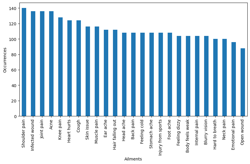
Figure 1: Class distribution of the ailments dataset (Mooney 2018)

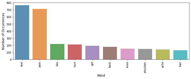
Figure 2: Top ten words mentioned by patients

Figure 3: An example record from the dataset (Mooney 2018)

Data Preprocessing

Converting textual data into digits is one of the main pillars of achieving natural language processing in various capacities (Mikolov et al. 2013). Therefore, the words must be expressed numerically to fit as inputs to deep learning models. Various methods are used to assess text corpus transformation into numerals, and each has its advantages and drawbacks. For instance, Term Frequency – Inverse Document Frequency (TF-IDF), one-hot encoding, and Word Embedding. The TF-IDF technique is used in text mining to reflect how important a word is to a document in corpus. One-Hot encoding splits a phrase’s words into a group and turns each word into a sequence of numbers regardless of meaning within the context (Shaaban, Hassan, and Guirguis 2022).

The word embedding technique, which is the focus of this work, differs from previously mentioned techniques as it represents each word by a vector of numbers indicating the semantic similarity between words. It creates a dense vector by transforming each word into a word vector that reflects its relative meaning within the document. The input is illustrated in a matrix $M\in\mathbb{R}^{n\times d}$, which denotes a collection of phrases. Each phrase $m\in M$ has a sequence of words: $w_{1}$,$w_{2}$,$w_{3}$, …,$w_{n}$; and every word is represented in a word vector of length $d$ (Shaaban, Hassan, and Guirguis 2022). Before applying the word embedding technique, we perform text preprocessing techniques, which involve tokenization, removal of stop words and lemmatization. First, each text is tokenized into words. Then, we remove stop words, which occur commonly across all texts. (e.g., ”the”, ”is”, ”you”). Next, we apply lemmatization for the sake of grouping different forms of the same word.

Long Short-Term Memory (LSTM)

Recurrent Neural Networks (RNN) is a deep learning approach introduced for modeling sequential data such as text, RNNs help predict what word or phrase will occur after a particular text, which could be a beneficial asset. This approach produces cutting-edge outcomes on text classification problems (Sherstinsky 2020).

Long Short-Term Memory (LSTM) is a type of RNN where LSTM cell blocks are in place of the standard neural network layers (Sherstinsky 2020). LSTM models have been shown to be capable of achieving remarkable text classification performance. LSTM cell consists of three different cells, namely the input, the forget and the output gates, which are used to determine which signals can be forwarded to the next node. Fig. 4 illustrates the structure of the LSTM cell. The hidden layer is connected to the input by a weight matrix $U$. $W$ represents the recurrent connection between the previous hidden layer and the current hidden layer. The candidate hidden state $\tilde{C}$ is computed using the current input and the previous hidden state. $C$ denotes the internal memory of the unit. It is a combination of the forget gate, multiplied by the previous memory, and the input gate, multiplied by the newly computed hidden state (Hochreiter and Schmidhuber 1997). The three gates: forget, input, and output, are represented in Fig. 4 as follows $f_{t}$, $i_{t}$, and $o_{t}$, respectively. Equations (1- 6) show the detailed workflow of LSTM cell.

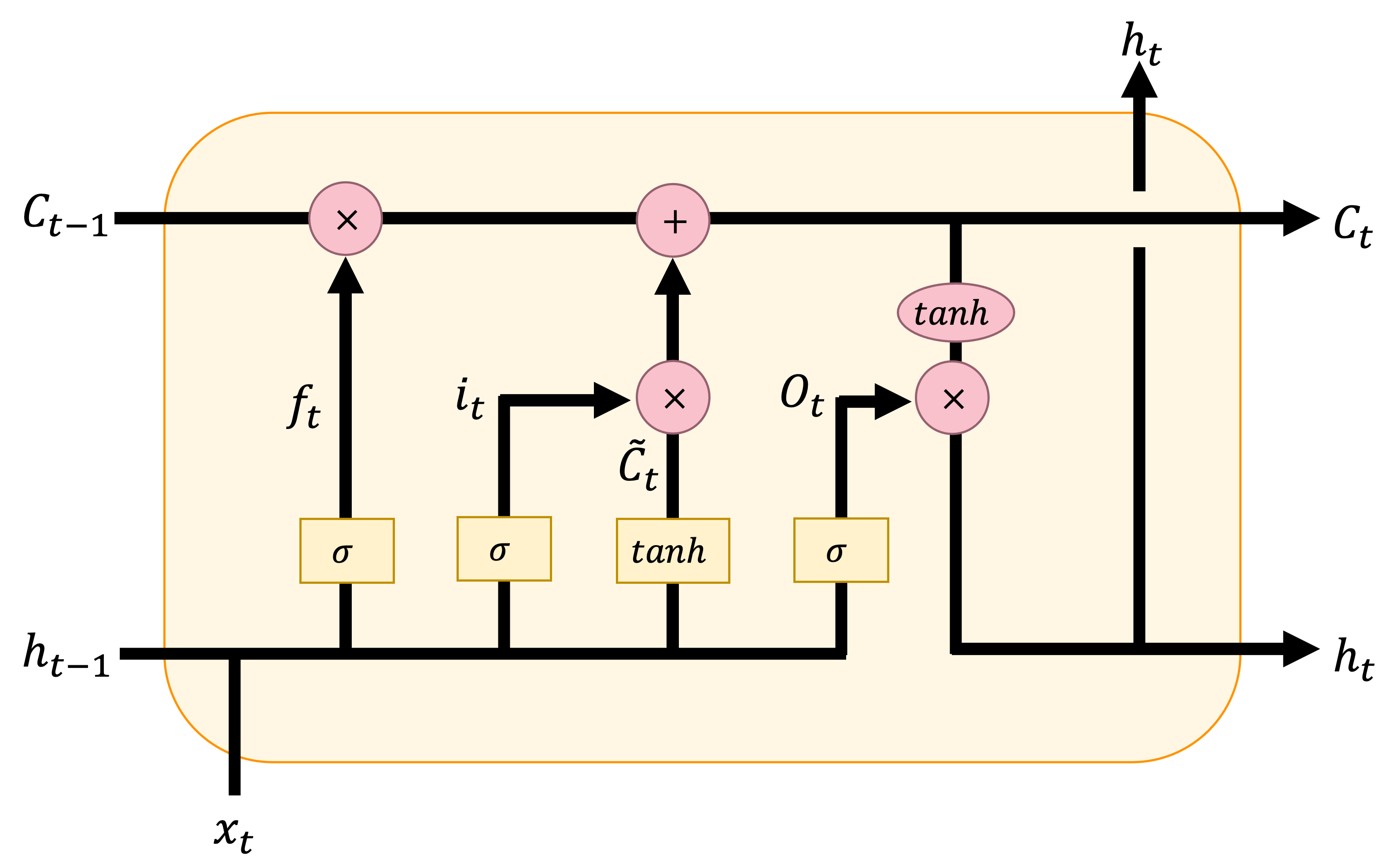
Figure 4: LSTM cell structure

$$i_{t}=\sigma\left(x_{t}U^{i}+h_{t-1}W^{i}\right)$$ (1)

$$f_{t}=\sigma\left(x_{t}U^{f}+h_{t-1}W^{f}\right)$$ (2)

$$o_{t}=\sigma\left(x_{t}U^{o}+h_{t-1}W^{o}\right)$$ (3)

$$\tilde{C}_{t}=tanh\left(x_{t}U^{g}+h_{t-1}W^{g}\right)$$ (4)

$$C_{t}=\sigma\left(f_{t}*C_{t-1}+i_{t}*\tilde{C}_{t}\right)$$ (5)

$$h_{t}=tanh(C_{t})*o_{t}$$ (6)

The Bees Algorithm

The Bees Algorithm (BA) is a swarm intelligence algorithm and a population-based algorithm that mimics the behavior of honey bees in nature in order to forage (Pham et al. 2006). In the beginning, scout bees are sent to discover the area. When those bees return, they perform a waggle dance that indicates the quality of the discovered batches. After that, recruiter bees are sent to the good batches to fetch good nectar, which enhances the quality and amount of produced honey. BA is started by initializing the population of $n$ number of bees. After that, the main loop of BA is started by selecting $m$ good bees out of $n$ bees to implement the local search. The local search exploits the found solutions in order to reach the optimal one. The elite bees $e$ are selected out of $m$ bees and they recruit $nep$ bees to help them find better solutions in their neighborhood. While $nsp$ bees are recruited to search in the neighborhood of the remaining good bees ($m-e$). In general, $nep$ should be greater than $nsp$. The remaining bees in the population implement the global search to explore all available solutions. This loop is repeated until convergence. The pseudo-code of BA is shown in Algorithm 1.

Algorithm 1 The Bees Algorithm

1:Input: $n$, $m$, $e$, $nep$, $nsp$, stopping criteria

2:Output: The optimal bee

3:Initialize a population of $n$ bees.

4:Calculate the fitness value for each bee in the population.

5:while stopping criteria are not satisfied do

6:     Sort bees with respect to their fitness values.

7:     Select $m$ good bees for local search.

8:     Select $e$ elite bees out of $m$ bees for local search.

9:     Recruit $nep$ bees for each of $e$ bees.

10:     Recruit $nsp$ bees for each of the remaining $m-e$ bees.

11:     Send the remaining $n-m$ bees for global search.

12:     Calculate the fitness value for all bees.

13:     Select the best bee as optimal.

14:end while

Hyperparameter Tuning using the Bees Algorithm

In this section, we introduce a novel framework called ”OptBA”, in which BA is applied to find the optimal values of LSTM hyperparameters: the number of epochs that the LSTM model needs to train and the number of units in LSTM layer. Thus, the structure of the bee in OptBA consists of the value of the number of epochs, the number of units and the accuracy value obtained from running LSTM as shown in Fig. 5. Considering that the remaining hyperparameters of LSTM are kept fixed during the experiment.

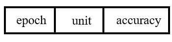
Figure 5: The formula of the bee in the proposed method. Each bee has three components: the two hyperparameters that are randomly chosen and one fitness value that is calculated

The algorithm starts by generating $n$ bees (solutions) randomly as the initial population, which represents $n$ different structures of LSTM. Each parameter is generated randomly using the Uniform distribution function by using the following equations.

$$epoch=uniform(epoch_{low},epoch_{high})$$ (7)

$$unit=uniform(unit_{low},unit_{high})$$ (8)

where:

1. $epoch_{low}$ and $epoch_{high}$ are the minimum and maximum values that can be assigned to the epoch parameter.

2. $unit_{low}$ and $unit_{high}$ are the minimum and maximum values that can be assigned to the number of units in LSTM.

After that, the evaluation function is implemented by training LSTM for each bee and the evaluation value is the obtained accuracy on the validation set. Next, these bees are ordered decently based on the resulting accuracy value. Then, the $m$ good bees are selected and the elite $e$ between them are distinguished. There are $nep$, and $nsp$ bees, which are recruited for each bee in the $m$ good bees and elite $e$, respectively, to enhance the found solution. This is performed by generating new values of the epoch and the unit parameters in the neighborhood of original values by using the Uniform distribution function. Equations (9- 10) illustrate the process:

$$epoch_{new}=uniform(epoch_{cur}-ngh,epoch_{cur}+ngh)$$ (9)

$$unit_{new}=uniform(unit_{cur}-ngh,unit_{cur}+ngh)$$ (10)

where:
$epoch_{cur}$ and $unit_{cur}$ are the current values of the current epoch and unit, and $epoch_{new}$ and $unit_{new}$ are the new values of the epoch and unit. Whereas, $ngh$ is the size of the neighborhood. The new bee is stored in the case of the new accuracy being greater than the accuracy of the original bee, which is the main function of the local search.

After implementing the local search, the global search is run for the remaining $(n-m)$ to discover new solutions that can be promised. The global search is implemented by replacing each remaining bee $(n-m)$ with a new one using the Equations (7- 8) as in initializing the population. Finally, the local search and the global search are repeated until the convergence or the maximum number of iterations of BA is reached. The detailed implementation of OptBA is in Algorithm 2.

Algorithm 2 The OptBA Algorithm

1:Input: $n$, $m$, $e$, $nep$, $nsp$, stopping criteria, word embeddings

2:Output: The optimal no. epochs and no. units

3:Initialize a population of $n$ LSTM models.

4:Train and evaluate each LSTM in the population.

5:while stopping criteria are not satisfied do

6:     Sort decently all models w.r.t their accuracy values.

7:     Select $m$ good models for local search.

8:     Select $e$ elite models for local search.

9:     Recruit $nep$ models for each of $e$ models.

10:     Recruit $nsp$ models for the remaining $m-e$ models.

11:     Send the remaining $n-m$ models for global search.

12:     Calculate the accuracy value for all models.

13:     Select the best model as optimal.

14:end while

Results and Discussion

In this section, we explore the ailment classification dataset (Mooney 2018) that contains 2829 unique text samples after performing data augmentation. First, data preprocessing techniques were applied including tokenization, stop words removal, and lemmatization. Next, textual data were transformed into a numerical format using the word embedding technique, where each word is represented by a vector of size 32. Then, we applied 10-fold cross-validation along with LSTM to predict the patient’s ailment. Additionally, we conduct ablation studies to justify the importance of tuning hyperparameters. Finally, we compare the model with SOTA. All experiments were run using Quadro RTX 6000 GPU with 24GB.

Model Configuration

Tab. 1 summarizes the configuration of LSTM hyperparameters: number of units, number of epochs, batch size, etc. Besides, Tab. 2 summarizes the values of each parameter of OptBA.

Table 1: Default hyperparameters setting of LSTM

Parameter	Value
No. units	64
No. epochs	20
Batch size	10
Dropout	0.2

Table 2: Settings of OptBA

Parameter	Value
Population size $n$	10
Good population size $m$	7
Elite population size $e$	3
Elite bees recruit $nep$	4
Good bees recruit $nsp$	2
Neighborhood size $ngh$	1

Evaluation Metrics

The performance of LSTM model was evaluated in Tab. 3 based on the following well-known metrics for multi-class classification:

• $T_{P}$: denotes true positives.

• $T_{N}$: denotes true negatives.

• $F_{P}$: denotes false positives.

• $F_{N}$: denotes false negatives.

• Precision: the proportion of the sum of true positive samples across all classes divided by the sum of true positive samples and false positive samples across all classes.

  $$Precision=\frac{T_{P}}{T_{P}+F_{P}}$$ (11)

• Recall: the proportion of the sum of true positive samples across all classes divided by the sum of true positive samples and false negative samples across all classes.

  $$Recall=\frac{T_{P}}{T_{P}+F_{N}}$$ (12)

• F1-score: is a weighted average of precision and recall.

  $$F1{\text{-}}Score=2\times\frac{Precision\times Recall}{Precision+Recall}$$ (13)

• Accuracy: compares the set of predicted labels to the corresponding set of actual labels.

  $$Accuracy=\frac{T_{P}+T_{N}}{T_{P}+F_{P}+T_{N}+F_{N}}$$ (14)

Table 3: Classification results of LSTM with default hyperparameters

Metric	Average weighted value
Precision	0.9837
Recall	0.9816
F1-score	0.9816
Accuracy	98.19%

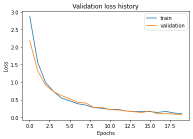
Figure 6: Training and validation curves of the LSTM model

As illustrated in Fig. 6, the training and validation curves for around $20$ epochs of training using the Adam optimizer (Kingma and Ba 2014) produced a well-generalized model.

To get the highest possible accuracy, we implemented OptBA to acquire the ideal hyperparameters for the LSTM model. Tab. 4 indicates that the performance increased significantly when the output dimensionality (the number of units) is adjusted to 108 along with running 49 epochs, which in return, increased the accuracy score by approximately 1.4% compared with the baseline model.

Table 4: The optimal hyperparameters for LSTM after running OptBA

Parameter	Value
No. epochs	49
No. units	108
Accuracy	99.63%

Table 5: Performance of LSTM with different numbers of epochs

No. epochs	Average accuracy%
10	96.07
20	98.16
30	98.69
40	98.40

Table 6: Performance of LSTM with different numbers of units

No. units	Average accuracy%
32	98.19
64	98.16
128	98.09

Table 7: Performance evaluation of Optuna and OptBA

Framework	Initial accuracy%	Best accuracy%	Best no. epochs	Best no. units	Parallel pruning	Profound search
Optuna	95.95	99.26	47	94	No	No
OptBA (ours)	99.63	99.63	49	108	Yes	Yes

Ablation Studies

Tab. 5 shows the effect of increasing the number of epochs manually from 10 to 40. Nevertheless, there is no significant improvement in the performance of LSTM after 20 epochs with 64 units, unlike the case of OptBA. Furthermore, Tab. 6 shows the outcomes of applying different numbers of LSTM units starting from 32 to 128. However, the best accuracy achieved was 98.19% by setting the number of units to 32 while fixing the number of training epochs to 20.

Comparison with Optuna

The architecture and the optimization techniques implemented by Optuna (Akiba et al. 2019) can generate one optimal solution per trial. In contrast, OptBA employs an optimization method that is a population-based search, allowing the pruning of suboptimal solutions to occur concurrently for accelerated convergence. However, direct comparison of total execution time is not feasible due to distinct numbers of solutions per trial and variations in search criteria between the two frameworks. For instance, OptBA swiftly identified the best solution in its initial trial and terminated early, whereas Optuna continued for 100 iterations without achieving the optimal outcome, as detailed in Tab 7. Moreover, the parameters of OptBA offer enhanced flexibility and depth in the quest for optimal solutions, without compromising the speed of evaluating an individual trial, but may require a larger number of trials. For example, setting $ngh=1$ entails a search extending one step forward and backward from the current optimal solution. The lower the $ngh$ value, the more profound search space. Consequently, OptBA guarantees to find the global optimal solution, distinguishing it from Optuna, which can get stuck in local optima as depicted in Tab. 7.

Conclusion

One of the drawbacks of deep learning models is that they require much effort in tuning hyperparameters. Therefore, the proposed work introduces a novel mechanism in order to obtain the optimal hyperparameters required for building deep neural networks. This mechanism utilizes the Bees Algorithm—one of the recent swarm intelligence algorithms that is adapted to work on Long Short-Term Memory (LSTM) for the aim of classifying ailments based on medical text. Experiments indicate that the Bees Algorithm can produce promising results and significantly improve the performance of deep neural networks. For future research, this work can be extended to explore other datasets as well as other deep learning models.

References

- Akiba et al. (2019) Akiba, T.; Sano, S.; Yanase, T.; Ohta, T.; and Koyama, M. 2019. Optuna: A next-generation hyperparameter optimization framework. In Proceedings of the 25th ACM SIGKDD international conference on knowledge discovery & data mining, 2623–2631.
- Al Hamoud, Hoenig, and Roy (2022) Al Hamoud, A.; Hoenig, A.; and Roy, K. 2022. Sentence subjectivity analysis of a political and ideological debate dataset using LSTM and BiLSTM with attention and GRU models. Journal of King Saud University - Computer and Information Sciences.
- Alsaleh and Larabi-Marie-Sainte (2021) Alsaleh, D.; and Larabi-Marie-Sainte, S. 2021. Arabic Text Classification Using Convolutional Neural Network and Genetic Algorithms. IEEE Access, 9: 91670–91685.
- Bakator and Radosav (2018) Bakator, M.; and Radosav, D. 2018. Deep learning and medical diagnosis: A review of literature. Multimodal Technologies and Interaction, 2(3): 47.
- Hochreiter and Schmidhuber (1997) Hochreiter, S.; and Schmidhuber, J. 1997. Long Short-Term Memory. Neural Computation, 9(8): 1735 – 1780.
- Kashkash, Haj Darwish, and Joukhdar (2022) Kashkash, M.; Haj Darwish, A.; and Joukhdar, A. 2022. new method to generate initial population of the Bees Algorithm for robot path planning in a static environment. In Pham, D.; and Hartono, N., eds., Intelligent Production and Manufacturing Optimisation - The Bees Algorithm Approach, chapter 12. Birmingham: Springer 2022., 1st edition.
- Khemapech, Sansrimahachai, and Toahchoodee (2019) Khemapech, I.; Sansrimahachai, W.; and Toahchoodee, M. 2019. Telemedicine - meaning, challenges and opportunities. Siriraj Medical Journal, 71(3): 246–252.
- Kingma and Ba (2014) Kingma, D. P.; and Ba, J. 2014. Adam: A method for stochastic optimization. arXiv preprint arXiv:1412.6980.
- Lotfi, Hamblin, and Rezaei (2020) Lotfi, M.; Hamblin, M. R.; and Rezaei, N. 2020. COVID-19: Transmission, prevention, and potential therapeutic opportunities.
- Ma (2019) Ma, E. 2019. NLP Augmentation. https://github.com/makcedward/nlpaug.
- Mikolov et al. (2013) Mikolov, T.; Chen, K.; Corrado, G.; and Dean, J. 2013. Efficient estimation of word representations in vector space. arXiv preprint arXiv:1301.3781.
- Mooney (2018) Mooney, P. 2018. Medical Speech, Transcription, and Intent. Accessed in 2022.
- Pham et al. (2006) Pham, D. T.; Ghanbarzadeh, A.; Koç, E.; Otri, S.; Rahim, S.; and Zaidi, M. 2006. The bees algorithm—a novel tool for complex optimisation problems. In Intelligent production machines and systems, 454–459. Elsevier.
- Piotrowski et al. (2017) Piotrowski, A. P.; Napiorkowski, M. J.; Napiorkowski, J. J.; and Rowinski, P. M. 2017. Swarm intelligence and evolutionary algorithms: Performance versus speed. Information Sciences, 384: 34–85.
- Shaaban, Hassan, and Guirguis (2022) Shaaban, M. A.; Hassan, Y. F.; and Guirguis, S. K. 2022. Deep convolutional forest: a dynamic deep ensemble approach for spam detection in text. Complex & Intelligent Systems, 1–13.
- Sherstinsky (2020) Sherstinsky, A. 2020. Fundamentals of recurrent neural network (RNN) and long short-term memory (LSTM) network. Physica D: Nonlinear Phenomena, 404: 132306.
- Wu and Deng (2019) Wu, H.; and Deng, Z. 2019. Do Physicians’ Online Activities Impact Outpatient Visits? An Examination of Online Health Communities Completed Research Paper. Technical report.
- Yu et al. (2019) Yu, Y.; Si, X.; Hu, C.; and Zhang, J. 2019. A review of recurrent neural networks: LSTM cells and network architectures. Neural computation, 31(7): 1235–1270.