Unbalanced and Light Optimal Transport

Abstract

While the field of continuous Entropic Optimal Transport (EOT) has been actively developing in recent years, it became evident that the classic EOT problem is prone to different issues like the sensitivity to outliers and imbalance of classes in the source and target measures. This fact inspired the development of solvers which deal with the unbalanced EOT (UEOT) problem $-$ the generalization of EOT allowing for mitigating the mentioned issues by relaxing the marginal constraints. Surprisingly, it turns out that the existing solvers are either based on heuristic principles or heavy-weighted with complex optimization objectives involving several neural networks. We address this challenge and propose a novel theoretically-justified and lightweight unbalanced EOT solver. Our advancement consists in developing a novel view on the optimization of the UEOT problem yielding tractable and non-minimax optimization objective. We show that combined with a light parametrization recently proposed in the field our objective leads to fast, simple and effective solver. It allows solving the continuous UEOT problem in minutes on CPU. We provide illustrative examples of the performance of our solver.

1 Introduction

During the recent years, the field of entropic optimal transport (Cuturi, 2013, EOT) has witnessed a lot of transformations. The majority of early works in the field are built upon solving the EOT problem between discrete probability measures (Peyré et al., 2019). Subsequently, the advances in the field of generative models have led to explosive interest from the ML community in developing the continuous EOT solvers, see (Gushchin et al., 2023b) for a survey. The setup of this problem assumes that the learner needs to estimate the EOT plan between continuous measures given only empirical samples of data from them. Such solvers found extensive applications in various areas, including image-to-image translation (Mokrov et al., 2024; Gushchin et al., 2023a), image generation (Wang et al., 2021; De Bortoli et al., 2021; Chen et al., 2021) and biological data transfer (Koshizuka & Sato, 2022; Vargas et al., 2021).

At the same time, various researches attract attention to the shortcomings of the classic EOT problem. In this formulation, EOT enforces hard constraints on the marginal measures, thus, does not allow for mass variations and sets equal weights for all samples. As a result, EOT shows high sensitivity to outliers and imbalance of classes in the source and target measures (Balaji et al., 2020) which are almost inevitable for large-scale datasets. In order to overcome these issues, it is common to consider extensions of EOT problem, e.g., unbalanced EOT (UEOT) (Chizat, 2017; Liero et al., 2018). The UEOT formulation allows for variation of total mass and individual samples’ weights by relaxing the marginal constraints through the use of divergences.

The scope of our paper is the continuous UEOT problem. It seems that in this field, a solver that is fast, light, and theoretically justified has not yet been developed. Indeed, many of the existing solvers follow a kind of heuristical principles and are based on the solutions of discrete OT. For example, (Lübeck et al., 2022) use a regression to interpolate the discrete solutions, and (Eyring et al., 2024) build a flow matching upon them. Almost all of the other solvers (Choi et al., 2023; Yang & Uhler, 2018) employ several neural networks with many hyper-parameters and require time-consuming optimization procedures. We solve the aforementioned shortcomings by introducing a novel lightweight solver which can play a role of simple baseline for unbalanced EOT.

Contributions. We develop a novel lightweight solver to estimate continuous unbalanced EOT couplings between probability measures (4). Our solver has a non-minimax optimization objective and employs the Gaussian mixture parametrization for the EOT plans. As a result, for measures of moderate dimensions. We experiment with our solver on illustrative synthetic tasks (5.1) and the unpaired image-to-image translation (5.2).

Notations. We work in the Euclidian space $(\mathbb{R}^{d},\|\cdot\|)$. We use $\mathcal{P}_{2,ac}(\mathbb{R}^{d})$ (or $\mathcal{M}_{2,+}(\mathbb{R}^{d})$) to denote the set of absolutely continuous Borel probability (or non-negative) measures on $\mathbb{R}^{d}$ with finite second moment and differential entropy. For any $p\in\mathcal{P}_{2,ac}(\mathbb{R}^{d})$ (or $\mathcal{M}_{2,+}(\mathbb{R}^{d})$), we use $p(x)$ to denote its density at a point $x\in\mathbb{R}^{d}$. For a given measure $\gamma\in\mathcal{M}_{2,+}(\mathbb{R}^{d}\times\mathbb{R}^{d})$, we denote its total mass by $\|\gamma\|_{1}\stackrel{{\scriptstyle\text{def}}}{{=}}\int_{\mathbb{R}^{d}}\gamma(x,y)dxdy$. We use $\gamma_{x}(x)$ and $\gamma_{y}(y)$ to denote the marginals of $\gamma(x,y)$. They statisfy the equality $\|\gamma_{x}\|_{1}=\|\gamma_{y}\|_{1}=\|\gamma\|_{1}$. We write $\gamma(y|x)$ to denote the conditional probability measure. Each such measure has a unit total mass. For two measures $p\in\mathcal{M}_{2,+}(\mathbb{R}^{d})$ and $q\in\mathcal{M}_{2,+}(\mathbb{R}^{d})$, the $f$-divergence between them is defined as $D_{f}\left(p\|q\right)\stackrel{{\scriptstyle\text{def}}}{{=}}\int_{\mathbb{R}^{d}}f(\nicefrac{{p(x)}}{{q(x)}})q(x)dx$. We use $\overline{f}$ to denote the Fenchel conjugate of a convex function $f$: $\overline{f}(t)=\sup_{u\in\mathbb{R}^{d}}\{ut-f(u)\}$. For two probability measures $p,q\in\mathcal{P}_{2,ac}(\mathbb{R}^{D})$, we use $\text{KL}\left(p\|q\right)$ to denote the Kullback-Leibler divergence between them. In turn, we use $H(p)$ to denote the differential entropy of $p$. To avoid any confusion, we apply KL or $H$ exclusively to probability measures.

2 Background

Here we give an overview of the relevant entropic optimal transport (EOT) concepts. For additional details on balanced EOT, we refer to (Cuturi, 2013; Genevay, 2019; Peyré et al., 2019), unbalanced EOT - (Chizat, 2017; Liero et al., 2018).

Unbalanced KL divergence and differential entropy. We start with recalling an auxiliary concept - the Unbalanced Kullback-Leibler divergence (UKL). For two positive measures $\gamma_{1},\gamma_{2}\in\mathcal{M}_{2,+}(\mathbb{R}^{d}\times\mathbb{R}^{d})$, UKL between them is

$$\text{UKL}\left(\gamma_{1}\|\gamma_{2}\right)\!\stackrel{{\scriptstyle\text{def}}}{{=}}\!\|\gamma_{1}\|_{1}\!\cdot\!\bigg{[}\!\text{KL}\left(\frac{\gamma_{1}}{\|\gamma_{1}\|_{1}}\|\frac{\gamma_{2}}{\|\gamma_{2}\|_{1}}\right)\!+\!h\big{(}\!\frac{\|\gamma_{2}\|_{1}}{\|\gamma_{1}\|_{1}}\!\big{)}\!\bigg{]},$$

where $h(a)\stackrel{{\scriptstyle\text{def}}}{{=}}a-1-\log a$. The latter is a convex and non-negative function attaining zero uniquely at $a=1$. KL term here is the usual Kullback-Leibler divergence computed between normalized measures, i.e., it is always non-negative and equals to zero only when $\gamma_{1}/\|\gamma_{1}\|_{2}=\gamma_{2}/\|\gamma_{2}\|_{2}$. Therefore, it follows that $\text{UKL}\left(\gamma_{1}\|\gamma_{2}\right)$ is always non-negative. Furthermore, it equals to zero only when $\gamma_{1}=\gamma_{2}$. These facts make UKL a valid measure of dissimilarity to compare two positive measures. In particular, when $\gamma_{1},\gamma_{2}$ are probability measures (i.e., $\|\gamma_{1}\|_{1}=\|\gamma_{2}\|_{1}$), UKL just coincides with the usual notion of KL.

For $\gamma\in\mathcal{M}_{2,+}(\mathbb{R}^{D})$ we define its unbalanced entropy:

$$H_{u}(\gamma)\stackrel{{\scriptstyle\text{def}}}{{=}}\|\gamma\|_{1}\big{[}H(\frac{\gamma}{\|\gamma\|_{1}})-h(\|\gamma\|_{1}^{-1})\big{]},$$

which boils to the usual differential entropy when $\|\gamma\|_{1}=1$.

Classic EOT formulation (with the quadratic cost). Consider two probability measures $p\!\in\!\mathcal{P}_{2,ac}(\mathbb{R}^{d})$, $q\!\in\!\mathcal{P}_{2,ac}(\mathbb{R}^{d})$. For $\varepsilon>0$, the EOT problem between $p$ and $q$ consists in finding a minimizer of

$$\min_{\pi\in\Pi(p,q)}\int_{\mathbb{R}^{d}}\int_{\mathbb{R}^{d}}\frac{\|x-y\|^{2}}{2}\pi(x,y)dxdy-\varepsilon H(\pi),$$ (1)

where $\Pi(p,q)$ is the set of probability measures $\pi\in\mathcal{P}_{2,ac}(\mathbb{R}^{d}\times\mathbb{R}^{d})$ with marginals $p$ and $q$ (transport plans), $H(\pi)$ is the differential entropy. Plan $\pi^{*}$ attaining the minimum exists, it is unique and called the EOT plan.

The EOT problem may be sensitive to outliers (Balaji et al., 2020) which are highly probable in real-world datasets. Moreover, it might not handle potential measure shifts such as class imbalances. Therefore, it is common to consider the unbalanced EOT problem (Yang & Uhler, 2018; Choi et al., 2023) which overcomes these issues by relaxing the marginal constraints (Séjourné et al., 2022).

Unbalanced EOT formulation (with the quadratic cost). Let $D_{f_{1}}$ and $D_{f_{2}}$ be two $f$-divergences over $\mathbb{R}^{d}$. For two probability measures $p\in\mathcal{P}_{2,ac}(\mathbb{R}^{d})$, $q\in\mathcal{P}_{2,ac}(\mathbb{R}^{d})$ and $\varepsilon>0$, the unbalanced EOT problem between $p$ and $q$ consists of finding a minimizer of

$$\inf_{\gamma\in\mathcal{M}_{2,+}(\mathbb{R}^{d}\times\mathbb{R}^{d})}\int_{\mathbb{R}^{d}}\int_{\mathbb{R}^{d}}\frac{\|x-y\|^{2}}{2}\gamma(x,y)dxdy-$$

$$\varepsilon H_{u}(\gamma)\!+\mathcal{D}_{f_{1}}(\gamma_{x},p)+\mathcal{D}_{f_{2}}(\gamma_{y},q).$$ (2)

Here the minimum is attained for a unique $\gamma^{*}$ which is called the unbalanced optimal entropic (UEOT) plan. Typical choices of $f_{i}$ are $f_{i}(x)=\lambda_{i}x\log x$ or $f_{i}(x)=\lambda_{i}(x-1)^{2}$ ($\lambda_{i}>0$) yielding the scaled KL and $\chi^{2}$ divergences, respectively.

Remark. The balanced EOT problem (1) is a special case of (2). Indeed, let $f_{1}$ and $f_{2}$ be the convex indicators of $\{1\}$, i.e., $f_{1}(x)=f_{2}(x)=\mathbb{I}_{x=1}\cdot 0+\mathbb{I}_{x\neq 1}\cdot\infty$. Then the $f$-divergences $D_{f_{1}}\left(\gamma_{x}\|p\right)$ and $D_{f_{2}}\left(\gamma_{y}\|q\right)$ become infinity if $p\neq\gamma_{x}$ or $q\neq\gamma_{y}$, and become zeros otherwise.

Dual form of unbalanced EOT problem (2) is

$$\!\sup_{(\phi,\psi)}\!\Bigg{\{}\!\!\!-\!\!\varepsilon\int_{\mathbb{R}^{d}}\int_{\mathbb{R}^{d}}\!\exp\{\frac{1}{\varepsilon}\!(\phi(x)+\psi(y)\!-\!\frac{\|x-y\|^{2}}{2})\}dxdy\!-\!$$

$$\int_{\mathbb{R}^{d}}\overline{f}_{1}(-\phi(x))p(x)dx\!-\!\int_{\mathbb{R}^{d}}\overline{f}_{2}(-\psi(y))q(y)dy\Bigg{\}}\stackrel{{\scriptstyle\text{def}}}{{=}}\mathcal{L}^{*}.\!$$ (3)

There exists a pair of optimal potentials $(\phi^{*},\psi^{*})$ delivering maximum to this problem. Optimal potentials have the following connection with the solution of the problem (2):

$$\gamma^{*}(x,y)\!=\!\exp\{\frac{\phi^{*}(x)}{\varepsilon}\}\!\exp\{-\frac{\|x-y\|^{2}}{2\varepsilon}\}\!\exp\{\frac{\psi^{*}(y)}{\varepsilon}\}.$$ (4)

Computational UEOT setup. Analytical solution for the unbalanced EOT problem is, in general, not known. Moreover, in real-world setups where unbalanced EOT is applicable, the measures $p$, $q$ are typically not available explicitly but only through their empirical samples (datasets). Below we summarize the learning setup which we consider.

We assume that data measures $p,q\in\mathcal{P}_{2,ac}(\mathbb{R}^{d})$ are unknown and accessible only by a limited number of i.i.d. empirical samples $\{x_{0},...,x_{N}\}\sim p$, $\{y_{0},...,y_{M}\}\sim q$. Our aim is to approximate the optimal UEOT plans solving (2) between the entire measures $p,q$. The recovered plans should allow the out-of-sample estimation, i.e., allow generating samples from $\gamma^{*}(\cdot|x^{\text{new}})$ where $x^{\text{new}}$ is a new test point (not necessarily present in the train data). Optionally, one may require the ability to sample from $\gamma^{*}_{x}$.

The described setup is typically called the continuous OT. It should not be twisted up with discrete OT setup (Peyré et al., 2019; Cuturi, 2013) where the aim is to recover the (unbalanced) EOT plan between the empirical measures $\hat{p}=\frac{1}{N}\sum_{i=1}^{N}\delta_{x_{i}}$, $\hat{q}=\frac{1}{M}\sum_{j=1}^{M}\delta_{y_{j}}$. There the out-of-sample estimations are typically not needed.

3 Related Work

	Problem	Principles	What recovers?	Limitations
(Yang & Uhler, 2018)	UOT	Solves $c$-trasform based semi-dual max-min reformulation of UOT using neural nets	Scaling factor $\nicefrac{{\gamma^{*}(x)}}{{p(x)}}$ and stochastic OT map $T^{*}(x,z)$	Complex max-min objective; 3 neural networks
(Lübeck et al., 2022)	Custom UOT	Regression on top of discrete EOT between re-balanced measures combined with ICNN-based solver (Makkuva et al., 2020)	Scaling factors and OT maps between re-scaled measures	Heuristically uses minibatch OT approximations
(Choi et al., 2023)	UOT	Solves semi-dual max-min reformulation of UOT using neural nets	Stochastic UOT map $T^{*}(x,z)$	Complex max-min objective; 2 neural networks
(Eyring et al., 2024)	UEOT	Flow Matching on top of discrete UEOT using neural nets	Parametrized vector field $(v_{t,\theta})_{t\in[0,1]}$ to transport the mass	Heuristically uses minibatch OT approximations
U-LightOT (ours)	UEOT	Solves non-minimax reformulation of dual UEOT using Gaussian Mixtures	Density of UEOT plan $\gamma^{*}$ together with light procedure to sample $x\sim\gamma^{*}_{x}(\cdot)$ and $y\sim\gamma^{*}_{y}(\cdot|x)$	Restricted to Gaussian Mixture parametrization

Table 1: Comparison of the principles of existing unbalanced OT/EOT solvers and our proposed light solver.

Nowadays, the sphere of continuous OT/EOT solvers is actively developing. Some of the early works related to this topic utilize OT cost as the loss function (Gulrajani et al., 2017; Genevay et al., 2018; Arjovsky et al., 2017). These approaches are not relevant to us as they do not learn OT/EOT maps (or plans). We refer to (Korotin et al., 2022) for a detailed review and bechmark of many of them.

At the same time, there exist a large amount of works within the discrete OT/EOT setup (Cuturi, 2013; Dvurechenskii et al., 2018; Xie et al., 2022; Nguyen et al., 2022), see (Peyré et al., 2019) for a survey. We again emphasize that solvers of this type are not relevant to us as they construct discrete matching between the given (train) samples and typically do not provide generalization to the new unseen (test) data. Only recently ML community has started developing out-of-sample estimation procedures based on discrete/batched OT. For example, (Fatras et al., 2020; Pooladian & Niles-Weed, 2021; Hütter & Rigollet, 2021; Deb et al., 2021; Manole et al., 2021; Rigollet & Stromme, 2022) mostly develop such estimators using the barycentric projections of the discrete EOT plans. Though these procedures have nice theoretical properties, their scalability remains unclear.

Balanced OT/EOT solvers. There exist a vast amount of neural solvers for continuous OT problem. Most of them learn the OT maps (or plans) via solving saddle point optimization problems (Asadulaev et al., 2024; Fan et al., 2023; Korotin et al., 2021; Gazdieva et al., 2022; Rout et al., 2022; Mokrov et al., 2024). Though the recent works (Gushchin et al., 2023a; Seguy et al., 2018; Daniels et al., 2021; Korotin et al., 2024) tackle the EOT problem (1), they consider its balanced version. Hence they are not relevant to us.

Among these works, only (Korotin et al., 2024) evades non-trivial training/inference procedures and is ideologically the closest to ours. In fact, our paper proposes the solver which subsumes their solver and generalizes it for the unbalanced case. The derivation of our solver is non-trivial and requires solid mathematical apparatus, see 4.

Unbalanced OT/EOT solvers. A vast majority of early works in this field tackle the discrete UOT/UEOT setup (Chapel et al., 2021; Fatras et al., 2021; Pham et al., 2020) but the principles under their construction are not easy to generalize to the continuous setting. Thus, many of the recent papers which tackle the continuous unbalanced OT/EOT setup employ the discrete solutions in the construction of their solvers. For example, (Lübeck et al., 2022) regress neural network on top of scaling factors obtained using the discrete UEOT while simultaneously learning the continuous OT maps using an ICNN method (Makkuva et al., 2020). In (Eyring et al., 2024), the authors implement Flow Matching (Lipman et al., 2022, FM) on top of the discrete UEOT plan. Despite the promising practical performance of these solvers, it is still unclear to what extent such approximations of UEOT plans are theoretically justified.

The recent papers (Yang & Uhler, 2018; Choi et al., 2023) are more related to our study as they do not rely on discrete OT approximations of the transport plan. However, they have non-trivial minimax optimization objectives solved using complex GAN-style procedures. Thus, these GANs often lean on the heavy neural parametrization, may incur instabilities during training and require careful hyperparameter selection (Lucic et al., 2018).

For completeness, we also mention other papers which are only slightly relevant to us. For example, (Gazdieva et al., 2023) consider incomplete OT which relaxes only one of the OT marginal constraints and is less general than the unbalanced OT. Other works (Dao et al., 2023; Balaji et al., 2020) incorporate unbalanced OT into the training objective of GANs aimed at generating samples from noise.

In contrast to the listed works, our paper proposes a theoretically justified and lightweight solver to the UEOT problem, see Table 1 for the detailed comparison of solvers.

4 Unbalanced and Light OT Solver

In this section, we derive the optimization objective (4.1) of our U-LightOT solver and present practical aspects of training and inference procedures (4.2). The proof for our theorem is given in Appendix A.

4.1 Derivation of the Optimization Objective

Following the learning setup described above, we aim to get a parametric approximation $\gamma_{\theta,w}$ of the UEOT plan $\gamma^{*}$. Here $\theta,\omega$ are the model parameters to learn and it will be clear later why we split them in two groups.

To recover $\gamma_{\theta,\omega}\approx\gamma^{*}$, our aim is to learn $\theta,\omega$ by directly minimizing the UKL divergence between $\gamma_{\theta,w}$ and $\gamma^{*}$:

$$\text{UKL}\left(\gamma^{*}\|\gamma_{\theta,\omega}\right)\rightarrow\min_{(\theta,\omega)}.$$ (5)

The main difficulty of this optimizing objective (5) is obvious: the UEOT plan $\gamma^{*}$ is unknown. Surprisingly, below we show that one still can optimize (5) without knowing $\gamma^{*}$.

Recall that the optimal UEOT plan $\gamma^{*}$ has the form (4). We first do some changes of variables. Specifically, we define $v^{*}(y)\stackrel{{\scriptstyle\text{def}}}{{=}}\exp\{\frac{2\psi^{*}(y)-\|y\|^{2}}{2\varepsilon}\}$. Formula (4) now reads as

$$\gamma^{*}(x,y)=\exp\{\frac{2\phi^{*}(x)-\|x\|^{2}}{2\varepsilon}\}\!\!\exp\{\frac{\langle x,y\rangle}{\varepsilon}\}v^{*}(y)\!\Longrightarrow$$

$$\!\!\!\gamma^{*}(y|x)\propto\exp\{\frac{\langle x,y\rangle}{\varepsilon}\}v^{*}(y).$$ (6)

Since the conditional plan has the unit mass, we may write

$$\gamma^{*}(y|x)=\exp\{\frac{\langle x,y\rangle}{\varepsilon}\}\frac{v^{*}(y)}{c_{v^{*}}(x)}$$ (7)

where $c_{v^{*}}(x)\stackrel{{\scriptstyle\text{def}}}{{=}}\int_{\mathbb{R}^{d}}\exp\{\frac{\langle x,y\rangle}{\varepsilon}\}v^{*}(y)dy$ is the normalization costant which ensures that $\int_{\mathbb{R}^{d}}\gamma^{*}(y|x)dy=1$.

Consider the decomposition $\gamma^{*}(x,y)=\gamma_{x}^{*}(x)\gamma^{*}(y|x)$. It shows that to obtain parametrization for the entire plan $\gamma^{*}(x)$, it is sufficient to consider parametrizations for its left marginal $\gamma^{*}_{x}$ and the conditional measure $\gamma^{*}(y|x)$. Meanwhile, equation (7) shows that conditional measures $\gamma^{*}(\cdot|x)$ are entirely described by the variable $v^{*}$. We use these observations to parametrize $\gamma_{\theta,w}$. We set

$$\gamma_{\theta,w}(x,y)\stackrel{{\scriptstyle\text{def}}}{{=}}u_{w}(x)\gamma_{\theta}(y|x)\!=\!u_{w}(x)\!\frac{\exp\{\nicefrac{{\langle x,y\rangle}}{{\varepsilon}}\}\!v_{\theta}(y)}{c_{\theta}(x)},\!$$ (8)

where $u_{w}$ and $v_{\theta}$ parametrize marginal measure $\gamma_{x}^{*}$ and the variable $v^{*}$, respectively. In turn, the constant $c_{\theta}(x)\stackrel{{\scriptstyle\text{def}}}{{=}}\int_{\mathbb{R}^{d}}\exp\{\frac{\langle x,y\rangle}{\varepsilon}\}v_{\theta}(y)dy$ is the parametrization of $c_{v^{*}}(x)$.

Next we demonstrate our main result which shows that the optimization of (5) can be done without the access to $\gamma^{*}$.

Theorem 4.1 (Tractable form of the UKL minimization).

Assume that $\gamma^{*}$ is parametrized using (8). Then the following bound holds: $\varepsilon\text{UKL}\left(\gamma^{*}\|\gamma_{\theta,w}\right)\!\leq\!\mathcal{L}(\theta,w)-\mathcal{L}^{*},$ where

$$\mathcal{L}(\theta,w)\stackrel{{\scriptstyle\text{def}}}{{=}}\int_{\mathbb{R}^{d}}\overline{f}_{1}(-\varepsilon\log\frac{u_{w}(x)}{c_{\theta}(x)}-\frac{\|x\|^{2}}{2})p(x)dx+$$

$$\int_{\mathbb{R}^{d}}\overline{f}_{2}(-\varepsilon\log v_{\theta}(y)-\frac{\|y\|^{2}}{2})q(y)dy+\varepsilon\|u_{w}\|_{1}$$ (9)

and constant $\mathcal{L}^{*}$ is the optimal value of the dual form (3).

The bound is tight in the sence that it turns to $0=0$ when $v_{\theta}(y)\!=\!\!\exp\{\frac{2\psi^{*}(y)-\|y\|^{2}}{2\varepsilon}\}$ and $u_{\omega}(x)\!=\!\!\exp\{\frac{2\phi^{*}(x)-\|x\|^{2}}{2\varepsilon}\}$.

In fact, equation (9) is the dual form (3) but with potentials $(\phi,\psi)$ expressed through $u_{\omega},v_{\theta}$ (and $c_{\theta}$).

$$\phi(x)\leftarrow\phi_{\theta,\omega}(x)=\varepsilon\log\frac{u_{w}(x)}{c_{\theta}(x)}+\frac{\|x\|^{2}}{2},$$

$$\psi(y)\leftarrow\psi_{\theta}(y)=\varepsilon\log v_{\theta}(y)+\frac{\|y\|^{2}}{2}$$

Our result can be interpreted as the bound on the quality of approximate solution $\gamma_{\theta,\omega}$ (2) recovered from the approximate solution to the dual problem (3). It can be directly proved using the original $(\phi,\psi)$ notation of the dual problem, but we use $(u_{\omega},v_{\theta})$ instead as with this change of variables the form of the recovered plan $\gamma_{\theta,\omega}$ is more interpretable ($u_{w}$ defines the first marginal, $v_{\theta}$ – conditionals).

Instead of optimizing (5) to get $\gamma_{\theta,\omega}$, we may optimize the obtained upper bound (9) which is more tractable. Indeed, (9) is a sum of the expectations w.r.t. the probability measures $p,q$. It means that we can use random samples to estimate (9) using Monte-Carlo estimation and optimize it with stochastic gradient descent procedure w.r.t. $(\theta,\omega)$. The main challenge here is the computation of the variable $c_{\theta}$ and term $\|u_{\omega}\|_{1}$. Below we show the smart parametrization by which both variables can be derived analytically.

4.2 Parameterization and the Optimization Procedure

Paramaterization. Recall that $u_{w}$ parametrizes the density of the marginal $\gamma^{*}_{x}$ which is unnormalized. Setting $x=0$ in equation (6), we get $\gamma^{*}(y|x=0)\propto v^{*}(y)$ which means that $v^{*}$ also corresponds to unnormalized density of the measure. These motivate us to use the unnormalized Gaussian mixture parametrization for the potential $v_{\theta}(y)$ and measure $u_{w}(x)$:

$$v_{\theta}(y)\!\!=\!\!\!\sum_{k=1}^{K}\!\!\alpha_{k}\mathcal{N}(y|r_{k},\!\varepsilon S_{k});$$

$$u_{\omega}(x)\!\!=\!\!\!\sum_{l=1}^{L}\!\beta_{l}\mathcal{N}(x|\mu_{l},\!\varepsilon\Sigma_{l}).\!$$ (10)

Here $\theta\stackrel{{\scriptstyle\text{def}}}{{=}}\{\alpha_{k},r_{k},S_{k}\}_{k=1}^{K}$, $w\stackrel{{\scriptstyle\text{def}}}{{=}}\{\beta_{l},\mu_{l},\Sigma_{l}\}_{l=1}^{L}$ with $\alpha_{k},\beta_{l}\geq 0$, $r_{k},\mu_{l}\in\mathbb{R}^{d}$ and $0\prec S_{k},\Sigma_{l}\in\mathbb{R}^{d\times d}$. Here covariance matrices are scaled by the $\varepsilon$ for convenience.

For this type of the parametrization, it obviously holds that $\|u_{w}\|_{1}=\sum_{l=1}^{L}\beta_{l}.$ Moreover, there exist closed-from expressions for the normalization constant $c_{\theta}(x)$ and conditional plan $\gamma_{\theta}(y|x)$, see (Korotin et al., 2024, Proposition 3.2). Specifically, define $r_{k}(x)\stackrel{{\scriptstyle\text{def}}}{{=}}r_{k}+S_{k}x$ and $\widetilde{\alpha}_{k}(x)\stackrel{{\scriptstyle\text{def}}}{{=}}\alpha_{k}\exp\{\frac{x^{T}S_{k}x+2r_{k}^{T}x}{2\varepsilon}\}$. It holds that

$$c_{\theta}(x)=\sum_{k=1}^{K}\widetilde{\alpha}_{k}(x);$$

$$\gamma_{\theta}(y|x)=\frac{1}{c_{\theta}(x)}\sum_{k=1}^{K}\widetilde{\alpha}_{k}(x)\mathcal{N}(y|r_{k}(x),\varepsilon S_{k}).$$ (11)

Using this result and (4.2), we get the expression for $\gamma_{\theta,w}$:

$$\gamma_{\theta,w}(x,y)=u_{\omega}(x)\cdot\gamma_{\theta}(y|x)=$$

$$\underbrace{\sum_{l=1}^{L}\!\beta_{l}\mathcal{N}(x|\mu_{l},\!\varepsilon\Sigma_{l})}_{u_{\omega}(x)}\cdot\underbrace{\frac{\sum_{k=1}^{K}\widetilde{\alpha}_{k}(x)\mathcal{N}(y|r_{k}(x),\varepsilon S_{k})}{\sum_{k=1}^{K}\widetilde{\alpha}_{k}(x)}}_{\gamma_{\theta}(y|x)}.$$ (12)

Training. We recall that the measures $p,q$ are accesible only by a number of empirical samples (see the learning setup in 2). Thus, given samples $\{x_{1},...,x_{N}\}$ and $\{y_{1},...,y_{M}\}$, we optimize the empirical analogue of (9)

$$\widehat{\mathcal{L}}(\theta,w)\stackrel{{\scriptstyle\text{def}}}{{=}}\frac{1}{N}\sum_{i=1}^{N}\overline{f}_{1}(-\varepsilon\log\frac{u_{w}(x_{i})}{c_{\theta}(x)}-\frac{\|x_{i}\|^{2}}{2})+$$

$$\frac{1}{M}\sum_{j=1}^{M}\overline{f}_{2}(-\varepsilon\log v_{\theta}(y_{j})-\frac{\|y_{j}\|^{2}}{2})\!+\!\varepsilon\|u_{w}\|_{1}$$ (13)

using minibatch gradient descent procedure w.r.t. parameters $(\theta,w)$. In the parametrization of $v_{\theta}$ and $u_{w}$ (4.2), we utilize the diagonal matrices $S_{k}$, $\Sigma_{k}$. This allows for decreasing the number of learnable parameters in $\theta$ and speeding up the computation of $S_{k}^{-1},\;\Sigma_{l}^{-1}$.

Inference. Our solver provides easy and lightweight sampling both from the marginal measure $u_{w}\approx\gamma_{x}^{*}$ and the conditional measure $\gamma_{\theta,w}(y|x)\approx\gamma^{*}(y|x)$ whose parameters are explicitly stated in equation (11).

4.3 Connection to Related Prior Works

The idea of using Gaussian Mixture parametrization for dual potentials in EOT-related tasks firstly appeared in the EOT/SB benchmark (Gushchin et al., 2023b). There it was used to obtain the benchmark pairs of probability measures with the known EOT solution between them. In (Korotin et al., 2024), the authors utilized this type of parametrization to obtain a light solver (LightSB) the balanced EOT.

Our approach for unbalanced EOT (9) subsumes their approach for balanced EOT. Specifically, our solver can be reduced to theirs by considering $\overline{f_{1}}(t)=t$ and $\overline{f_{2}}(t)=t$ in the equation (9). Namely, objective (9) becomes

$$\mathcal{L}(\theta,w)=\int_{\mathbb{R}^{d}}(-\varepsilon\log\frac{u_{w}(x)}{c_{\theta}(x)}-\frac{\|x\|^{2}}{2})p(x)dx+$$

$$\int_{\mathbb{R}^{d}}(-\varepsilon\log v_{\theta}(y)-\frac{\|y\|^{2}}{2})q(y)dy+\varepsilon\|u_{w}\|_{1}=$$

$$-\varepsilon\big{(}\int_{\mathbb{R}^{d}}\log\frac{u_{w}(x)}{c_{\theta}(x)})p(x)dx+\int_{\mathbb{R}^{d}}\log v_{\theta}(y)q(y)dy\big{)}-$$

$$\|u_{w}\|_{1}+\underbrace{\int_{\mathbb{R}^{d}}\frac{\|x\|^{2}}{2}p(x)dx-\int_{\mathbb{R}^{d}}\frac{\|y\|^{2}}{2}q(y)dy}_{\stackrel{{\scriptstyle\text{def}}}{{=}}C(p,q)}=$$

$$\varepsilon\big{(}\int_{\mathbb{R}^{d}}\log c_{\theta}(x)p(x)dx-\int_{\mathbb{R}^{d}}\log v_{\theta}(y)q(y)dy\big{)}-$$ (14)

$$\varepsilon\int_{\mathbb{R}^{d}}\log u_{w}(x)p(x)dx+\|u_{w}\|_{1}+C(p,q).$$ (15)

Note that here line (14) depends exclusively on $\theta$ and line (15) on $\omega$. Furthermore, line (14) exactly coincides with the LightSB’s objective, see (Korotin et al., 2024, Proposition 8). Also note that the minimum of line (15) is attained when $u_{w}=p$ and this part is not actually needed in the balanced case, see (Korotin et al., 2024, Appendix C).

5 Experimental Illustrations

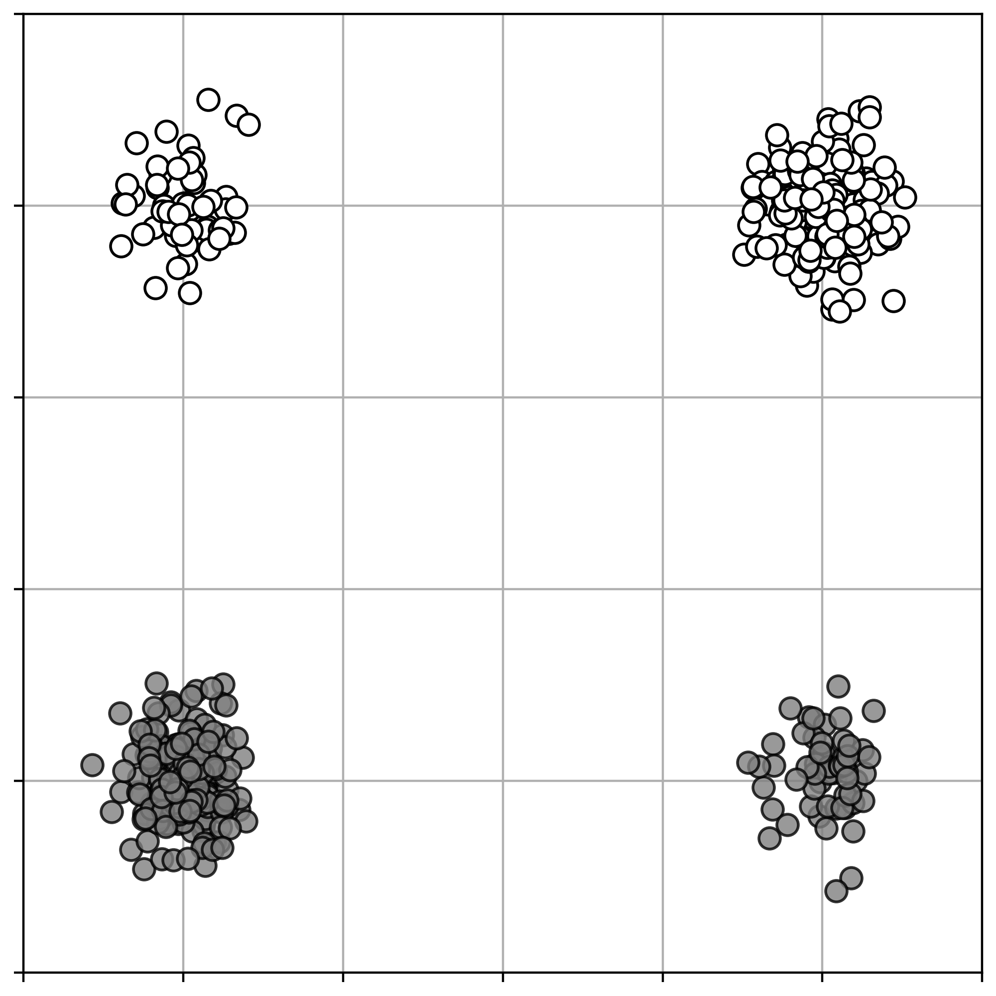
(a) Input, target measures

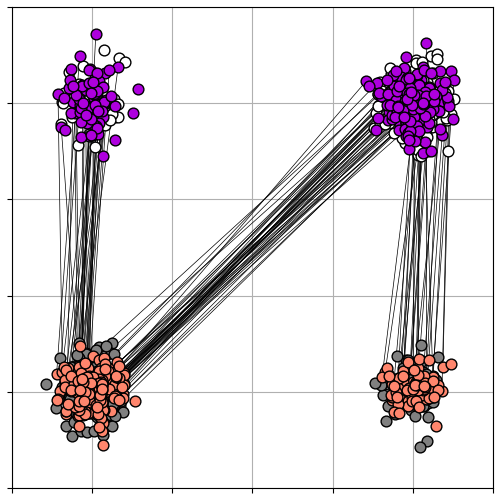
(b) LightSB

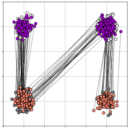
(c) Interpolation

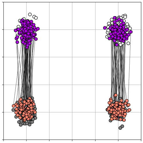
(d) U-LightOT (ours)

Figure 1: Conditional plans $\gamma_{\theta,\omega}(y|x)$ learned by our solver in Gaussians experiment. Here $p_{\omega}$ denotes the normalized first marginal $u_{w}$, i.e., $p_{\omega}=u_{\omega}/\|u_{\omega}\|_{1}$.

In this section, we test our solver on the synthetic task (5.1) and unpaired image translation (5.2). The code is written using PyTorch framework and will be made public. The experiments are issued in the form of *.ipynb notebooks. Each experiment requires several minutes of training on CPU with 4 cores.

5.1 Example with the Mixture of Gaussians

In this section, we provide ’Gaussians’ example in 2D to demonstrate the ability of our solver to deal with the imbalance of classes in the source and target measures. We follow the idea of the experimental setup proposed in (Eyring et al., 2024, Figure 2). Both probability measures $p$ and $q$ are the mixtures of Gaussians, see Figure 1(a). The difference is in the masses of the individual Gaussians, i.e.,

$$p(x)\!=\!\frac{1}{4}\mathcal{N}(x|(-2,3),0.1\cdot I_{2})\!+\!\frac{3}{4}\mathcal{N}(x|(1,3),0.1\cdot I_{2})$$

$$q(y)\!=\!\frac{3}{4}\mathcal{N}(y|(-2,0),0.1\cdot I_{2})\!+\!\frac{1}{4}\mathcal{N}(y|(1,0),0.1\cdot I_{2})$$

Baselines. We consider (Korotin et al., 2024, LightSB) as the main baseline which computes balanced EOT maps between the measures. In Figure 1(a), we show that it fails to transport the mass from the input Gaussians to the closest target ones due to the imbalance of their masses. In fact, as we wrote in Section 4.3, LightSB is a special balanced case of our solver given the $f$-divergences $\overline{f_{1}}(t)=\overline{f_{2}}(t)=t$.

In Figure 1(d), we demonstrate the results of our U-LightOT solver $\overline{f_{1}},\overline{f_{2}}$ defined as the $\text{SoftPlus}(t)=\log(1+\exp^{t})$ function. In this case, our solver successfully overcomes the imbalance issue and transports the mass correctly.

For completeness, we also present a kind of interpolation between the balanced and SoftPlus cases. We consider $\overline{f_{1}}(t)=\overline{f_{2}}(t)=\frac{1}{2}t+\frac{1}{2}\text{SoftPlus}(t)$. In Figure 1(c), we see that for the mass is not transported correctly. However, the amount of incorrecly mapped points is less than in the balanced (LightSB) case (Figure 1(d)).

Remark. We conduct all experiments here with the entropy regularization parameter $\varepsilon=0.05$. The parameter $\varepsilon$ is resposible for the stochasticity of the learned transport $\gamma_{\theta}(\cdot|x)$. Since we are mostly interested in the correct transport of the mass (controlled by $f_{1},f_{2}$) rather than the stochasticity, we do not pay much attention to $\epsilon$ throughout the paper.

5.2 Unpaired Image-to-Image Translation

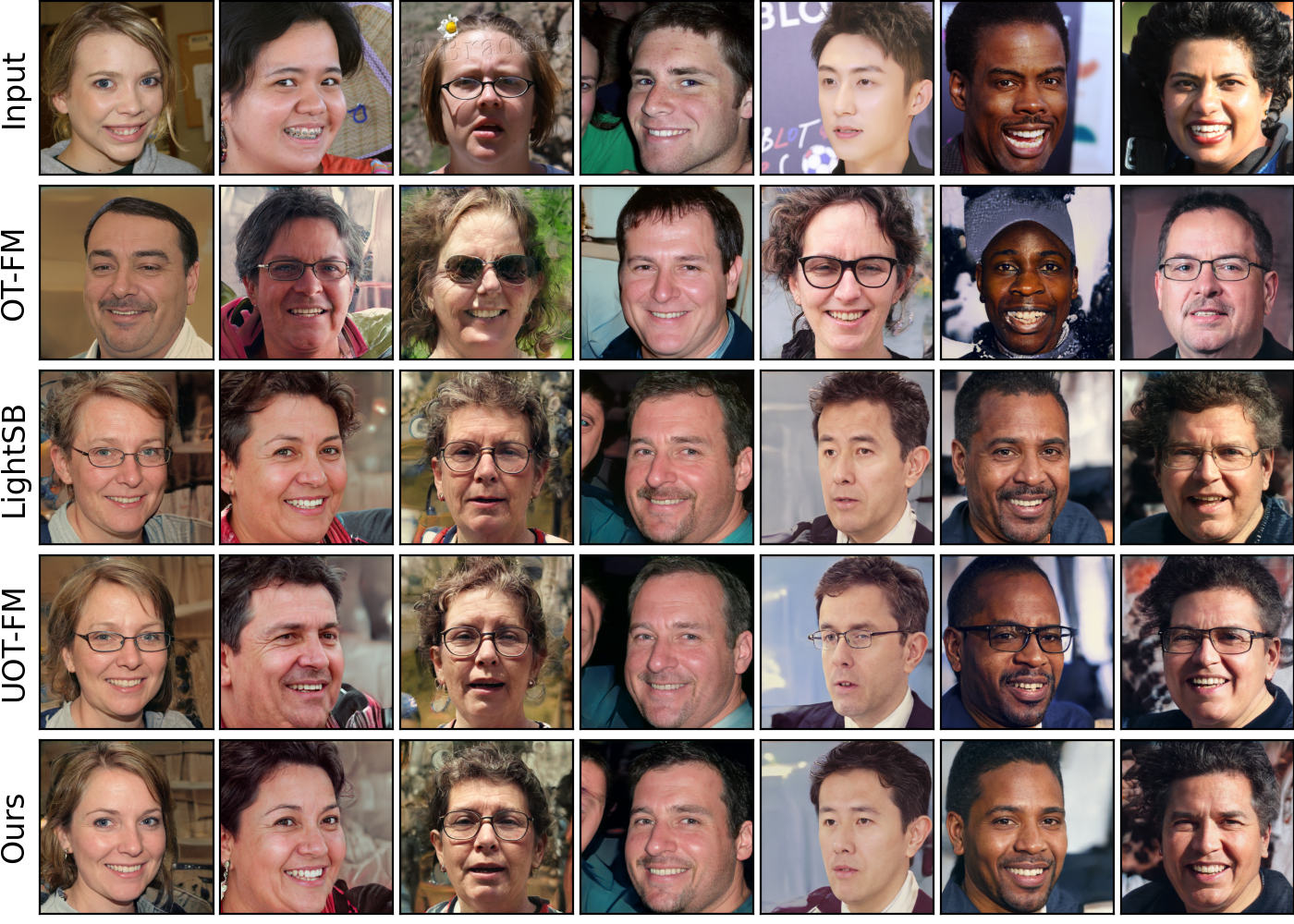
(a) Young $\rightarrow$ Adult

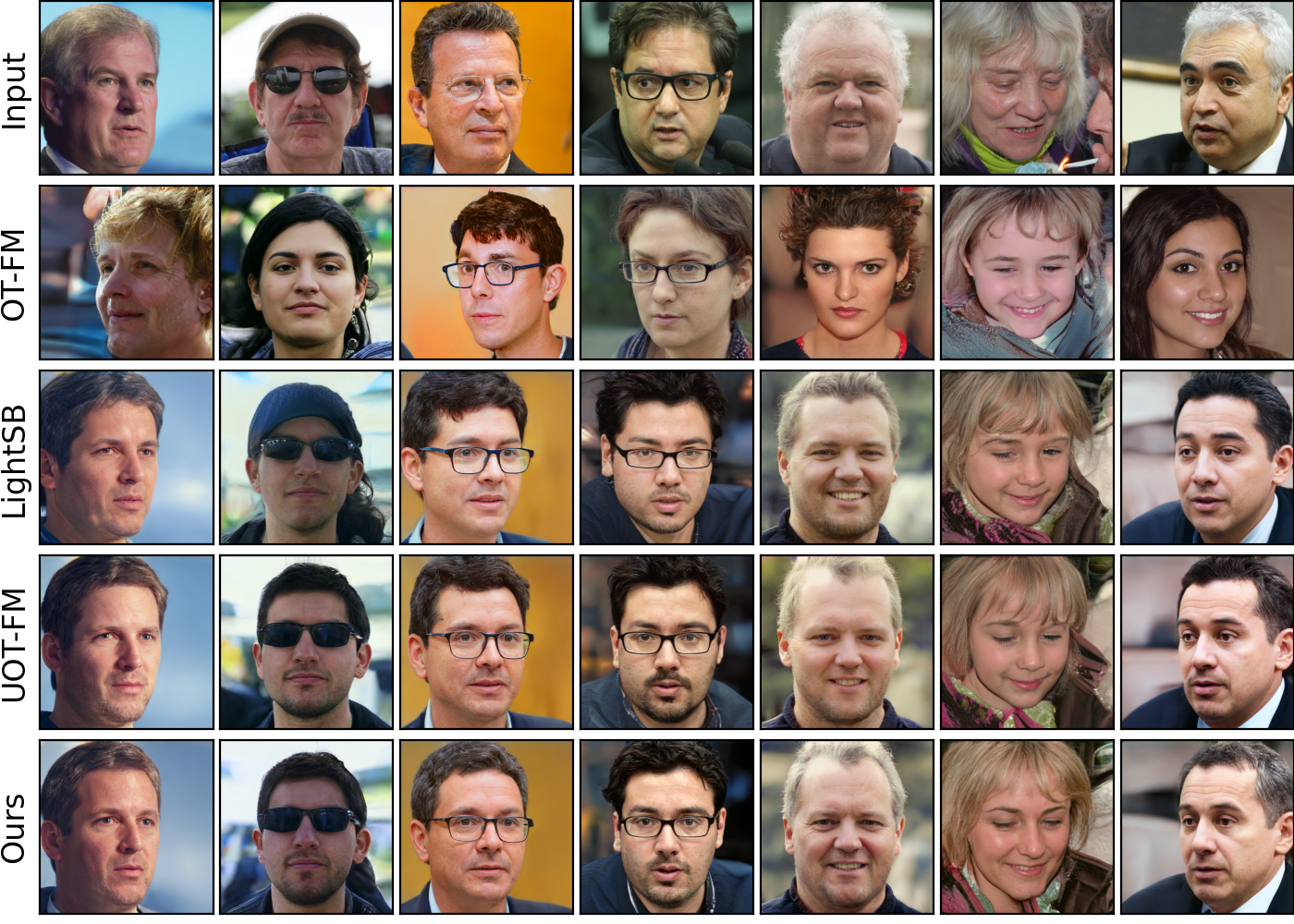
(b) Adult $\rightarrow$ Young

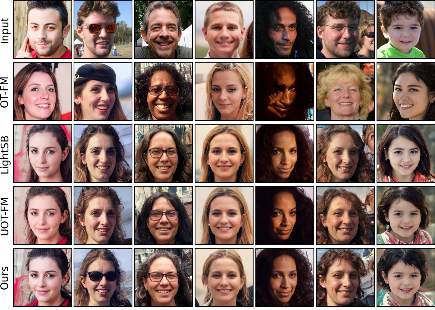
(c) Man $\rightarrow$ Woman

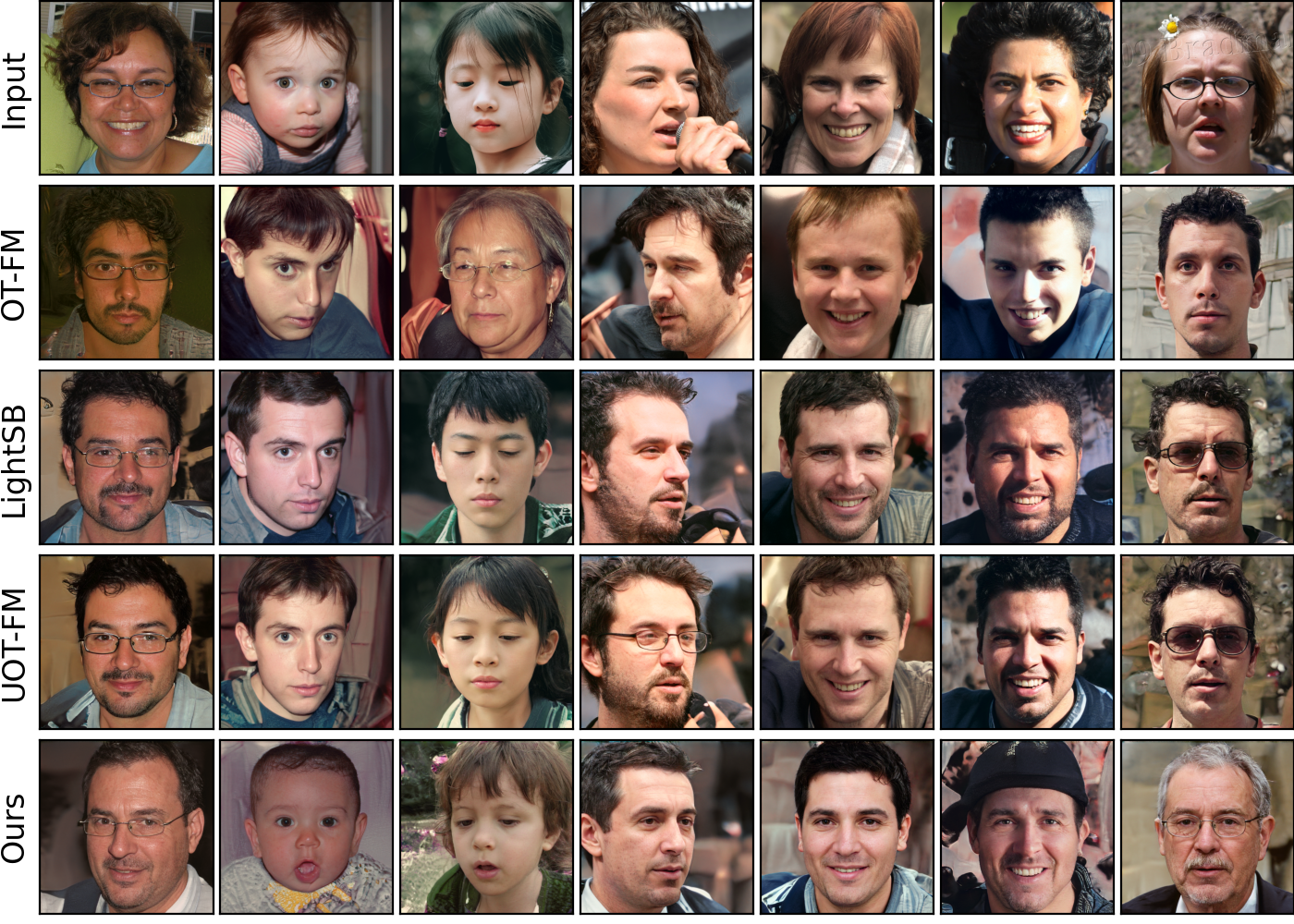
(d) Woman $\rightarrow$ Man

Figure 2: Unpaired translation with LightSB, OT-FM, UOT-FM and our U-LightOT solver applied in the latent space of ALAE for FFHQ images (1024$\times$1024).

In this section, we consider the image-to-image translation task (Zhu et al., 2017). We follow the experimental setup of (Korotin et al., 2024, Section 5.4) and use pre-trained ALAE autoencoder (Pidhorskyi et al., 2020) for $1024\times 1024$ FFHQ dataset (Karras et al., 2019) of human faces. We consider different variants of translation: adult$\leftrightarrow$young and woman$\leftrightarrow$man. We split the data on train and test part following (Korotin et al., 2024) and use their $512$-dimensional latent codes extracted for images in each domain.

Class	Man	Woman
Young	$15K$	$23K$
Adult	$7K$	$3.5K$

Table 2: Number of train FFHQ images for each class.

The challenge of the described translations lies in the imbalance of classes in the measures of source and target images, see Table 2. Indeed, let us consider in more details adult$\rightarrow$young translation. In FFHQ dataset, the amount of adult input images labeled as woman significantly outnumbers adults labeled as man. The situation is opposite for the target (young) data. Thus, solvers based on the balanced transport are expected to translate some of the young woman faces to the adult man ones. At the same time, solvers based on unbalanced transport are expected to solve this issue.

Baselines. We perform comparison with the recent procedure (Eyring et al., 2024, UOT-FM) which considered roughly the same setup and demonstrated good performance. This method interpolates the results of unbalanced discrete OT to the continuous setup using the flow matching (Lipman et al., 2022). For completeness, we include the comparison with LightSB and balanced optimal transport-based flow matching (OT-FM) (Lipman et al., 2022) to demonstrate the issues of the balanced solvers. Qualitative results for OT-FM, LightSB and our U-LightOT solver are given in Figure 2. Additional qualitative results are given in Appendix C.

Metrics. Our aim is to assess the ability of the solvers to perform the translation of latent codes keeping the class of the input images unchanged, e.g., in adult$\rightarrow$young translation, the gender should not be changed. We train a $99\%$ MLP classifier on the images of different classes and compute the accuracy between the actual classes of the input images and those of the generated ones. The results are given in Table 3 and show that our solver outperforms its alternatives in dealing with class imbalance issue.

Translation	OT-FM	LightSB	UOT-FM	U-LightOT (ours)
Young$\rightarrow$Adult	60.71	87.11	87.72	94.92
Adult$\rightarrow$Young	56.75	76.68	81.34	95.39
Man$\rightarrow$Woman	73.82	81.33	87.35	92.80
Woman$\rightarrow$Man	77.56	83.29	88.20	95.17

Table 3: Accuracy of keeping the class of the input image.

6 Discussion

Potential impact. Our light and unbalanced solver has a lot of advantages in comparison with the other existing UEOT solvers. First, it does not require complex max-min optimization. Second, it provides the closed form of the conditional measures $\gamma_{\theta,\omega}(y|x)\approx\gamma^{*}(y|x)$ of the UEOT plan. Moreover, it allows for sampling both from the conditional measure $\gamma_{\theta,\omega}(y|x)$ and marginal measure $u_{w}(x)\approx\gamma_{x}(x)$. Besides, the decisive superiority of our lightweight and unbalanced solver is its simplicity and convenience of using. Indeed, it has a straightforward and non-minimax optimization objective and avoids heavy neural parametrization. As a result, our lighweight and unbalanced solver converges in minutes on CPU. We expect that these advantages could boost the usage of our solver as a standard and easy baseline for UEOT task with applications in different spheres.

Limitations. One limitation of our solver is the usage of the Gaussian Mixture parametrization which might restrict the scalability of our solver. This points to the necessity for developing ways to optimize objective (3) with more general parametrization, e.g., neural networks. This is a promising avenue for future work.

7 Broader impact

This paper presents work whose goal is to advance the field of Machine Learning. There are many potential societal consequences of our work, none of which we feel must be specifically highlighted here.

Appendix A Proofs

Proof of Theorem 4.1.

To begin with, we derive the useful property of the optimal UEOT plans. We recall that $\phi^{*}$ and $\psi^{*}$ are the minimizers of dual form (3), i.e., $(\phi^{*},\psi^{*})\in\operatorname*{arg\,min}_{(\phi,\psi)}\mathcal{J}(\phi,\psi)$ where

$$\mathcal{J}(\phi,\psi)\stackrel{{\scriptstyle\text{def}}}{{=}}\varepsilon\int_{\mathbb{R}^{d}}\int_{\mathbb{R}^{d}}\!\exp\{\frac{1}{\varepsilon}\!(\phi(x)+\psi(y)\!-\!\nicefrac{{\|x-y\|^{2}}}{{2}})\}dxdy\!+\int_{\mathbb{R}^{d}}\overline{f}_{1}(-\phi(x))p(x)dx\!+\!\int_{\mathbb{R}^{d}}\overline{f}_{2}(-\psi(y))q(y)dy.$$

Then, by the first order optimality condition $\frac{d}{d\phi}\mathcal{J}(\phi,\psi)|_{\phi=\phi^{*}}=0$ and $\frac{d}{d\psi}\mathcal{J}(\phi,\psi)|_{\psi=\psi^{*}}\!=\!0$. It means that

$$\frac{d}{d\phi}\mathcal{J}(\phi,\psi)|_{\phi=\phi^{*}}(x)=\cancel{\varepsilon\cdot\varepsilon^{-1}}\int_{\mathbb{R}^{d}}\exp\{\varepsilon^{-1}(\phi^{*}(x)+\psi^{*}(y)-\nicefrac{{\|x-y\|^{2}}}{{2}})\}dy-\nabla\overline{f}_{1}(-\phi^{*}(x))p(x)=0\Longrightarrow$$

$$\nabla\overline{f}_{1}(-\phi^{*}(x))=\frac{\gamma^{*}_{x}(x)}{p(x)}$$ (16)

holds for all $x$, s.t. $p(x)>0$. Analogously, we get that $\nabla\overline{f}_{2}(-\psi^{*}(y))=\frac{\gamma^{*}_{y}(y)}{q(y)}$ for all $y$, s.t. $q(y)>0$.

For convenience of the further derivations, we consider the change of variables to simplify the expression for $\mathcal{L}(\theta,\omega)$. We define $\phi_{\theta,\omega}(x)\stackrel{{\scriptstyle\text{def}}}{{=}}\varepsilon\log\frac{u_{\omega}(x)}{c_{\theta}(x)}-\frac{\|x\|^{2}}{2}$ and $\psi_{\theta}(y)\stackrel{{\scriptstyle\text{def}}}{{=}}\varepsilon\log v_{\theta}(y)-\frac{\|y\|^{2}}{2}$. Then

$$\mathcal{L}(\theta,\omega)=\int_{\mathbb{R}^{d}}\overline{f}_{1}(-\phi_{\theta,\omega}(x))p(x)dx+\int_{\mathbb{R}^{d}}\overline{f}_{2}(-\psi_{\theta}(y))q(y)dy+\varepsilon\|u_{w}\|_{1}=\mathcal{J}(\phi_{\theta,\omega},\psi_{\omega}).$$

Next, we simplify our main objective:

$$\text{UKL}\left(\gamma^{*}\|\gamma_{\theta,\omega}\right)\!=\!\|\gamma^{*}\|_{1}\bigg{[}\text{KL}\left(\frac{\gamma^{*}}{\|\gamma^{*}\|_{1}}\|\frac{\gamma_{\theta,\omega}}{\|\gamma_{\theta,\omega}|_{1}}\right)+\frac{\|\gamma_{\theta,\omega}\|_{1}}{\|\gamma^{*}\|_{1}}\!-\!1\!-\!\log\frac{\|\gamma_{\theta,\omega}\|_{1}}{\|\gamma^{*}\|}\bigg{]}\!=\!$$

$$\cancel{\|\gamma^{*}\|_{1}\!\cdot\!\|\gamma^{*}\|_{1}^{-1}}\Bigg{(}\int_{\mathbb{R}^{d}\times\mathbb{R}^{d}}\!\!\!\gamma^{*}(x,y)\log\gamma^{*}(x,y)dxdy-\int_{\mathbb{R}^{d}\times\mathbb{R}^{d}}\gamma^{*}(x,y)\log\|\gamma^{*}\|_{1}dxdy-\int_{\mathbb{R}^{d}\times\mathbb{R}^{d}}\!\!\!\gamma^{*}(x,y)\log\gamma_{\theta,\omega}(x,y)dxdy+$$

$$\int_{\mathbb{R}^{d}\times\mathbb{R}^{d}}\gamma^{*}(x,y)\log\|\gamma_{\theta,\omega}\|_{1}dxdy+\|\gamma_{\theta,\omega}\|_{1}-\|\gamma^{*}\|_{1}-\|\gamma^{*}\|_{1}\log\frac{\|\gamma_{\theta,\omega}\|_{1}}{\|\gamma^{*}\|_{1}}\Bigg{)}=\int_{\mathbb{R}^{d}\times\mathbb{R}^{d}}\gamma^{*}(x,y)\log\gamma^{*}(x,y)dxdy-\!$$

$$\cancel{\|\gamma^{*}\|_{1}\log\|\gamma^{*}\|_{1}}\!-\int_{\mathbb{R}^{d}\times\mathbb{R}^{d}}\!\!\!\gamma^{*}(x,y)\log\gamma_{\theta,\omega}(x,y)dxdy+\cancel{\|\gamma^{*}\|_{1}\log\|\gamma_{\theta,\omega}\|_{1}}\!+\!\|\gamma_{\theta,\omega}\|_{1}-\|\gamma^{*}\|_{1}-\cancel{\|\gamma^{*}\|_{1}\log\|\gamma_{\theta,\omega}\|_{1}}+$$

$$\cancel{\|\gamma^{*}\|_{1}\log\|\gamma^{*}\|_{1}}=\int_{\mathbb{R}^{d}\times\mathbb{R}^{d}}\gamma^{*}(x,y)\log\gamma^{*}(x,y)dxdy-\int_{\mathbb{R}^{d}\times\mathbb{R}^{d}}\!\!\!\gamma^{*}(x,y)\log\gamma_{\theta,\omega}(x,y)dxdy+\!\|\gamma_{\theta,\omega}\|_{1}-\|\gamma^{*}\|_{1}.$$ (17)

Now we recall that the ground-truth UEOT plan $\gamma^{*}(x,y)$ and the optimal dual variables $\phi^{*}(x)$, $\psi^{*}(y)$ are connected via equation (4). Similarly, our parametrized plan $\gamma_{\theta,\omega}(x,y)$ can be expressed using $\phi_{\theta,\omega}(x)$, $\psi_{\theta}(y)$ as $\gamma_{\theta,\omega}(x,y)=\exp\{\varepsilon^{-1}(\phi_{\theta,\omega}(x)+\psi_{\theta}(y)-\nicefrac{{\|x-y\|^{2}}}{{2}})\}$. Then

$$\eqref{ukl-derivation-bgt}=\varepsilon^{-1}\int_{\mathbb{R}^{d}\times\mathbb{R}^{d}}\gamma^{*}(x,y)\big{(}\phi^{*}(x)+\psi^{*}(y)-\nicefrac{{\|x-y\|^{2}}}{{2}}\big{)}dxdy-\varepsilon^{-1}\int_{\mathbb{R}^{d}\times\mathbb{R}^{d}}\gamma^{*}(x,y)\big{(}\phi_{\theta,\omega}(x)+\psi_{\theta}(y)-\nicefrac{{\|x-y\|^{2}}}{{2}}\big{)}dxdy+$$

$$\|\gamma_{\theta,\omega}\|_{1}-\|\gamma^{*}\|_{1}=\varepsilon^{-1}\int_{\mathbb{R}^{d}\times\mathbb{R}^{d}}\gamma^{*}(x,y)\big{(}\phi^{*}(x)+\psi^{*}(y)-\phi_{\theta,\omega}(x)-\psi_{\theta}(y)\big{)}dxdy+\|\gamma_{\theta,\omega}\|_{1}-\|\gamma^{*}\|_{1}=$$

$$\varepsilon^{-1}\int_{\mathbb{R}^{d}}\gamma^{*}_{x}(x)\big{(}\phi^{*}(x)-\phi_{\theta,\omega}(x)\big{)}dx+\varepsilon^{-1}\int_{\mathbb{R}^{d}}\gamma^{*}_{y}(y)\big{(}\psi^{*}(y)-\psi_{\theta}(y)\big{)}dy+\|\gamma_{\theta,\omega}\|_{1}-\|\gamma^{*}\|_{1}.$$ (18)

Finally, we derive

$$\eqref{ukl-derivation-bc}=\varepsilon^{-1}\int_{\mathbb{R}^{d}}\!\!\!\!\underbrace{\frac{\gamma^{*}_{x}(x)}{p(x)}}_{\nabla\overline{f}_{1}(-\phi^{*}(x))}\!\!\!\!\!\big{(}\phi^{*}(x)-\phi_{\theta,\omega}(x)\big{)}p(x)dx+\varepsilon^{-1}\int_{\mathbb{R}^{d}}\underbrace{\frac{\gamma^{*}_{y}(y)}{q(y)}}_{\nabla\overline{f}_{2}(-\psi^{*}(y))}\!\!\!\big{(}\psi^{*}(y)-\psi_{\theta}(y)\big{)}q(y)dy+\|\gamma_{\theta,\omega}\|_{1}-\|\gamma^{*}\|_{1}=$$

$$\varepsilon^{-1}\int_{\mathbb{R}^{d}}\nabla\overline{f}_{1}(-\phi^{*}(x))\big{(}\phi^{*}(x)-\phi_{\theta,\omega}(x)\big{)}p(x)dx+\varepsilon^{-1}\int_{\mathbb{R}^{d}}\nabla\overline{f}_{2}(-\psi^{*}(y))\big{(}\psi^{*}(y)-\psi_{\theta}(y)\big{)}q(y)dy+\|\gamma_{\theta,\omega}\|_{1}-\|\gamma^{*}\|_{1}\leq$$ (19)

$$\varepsilon^{-1}\int_{\mathbb{R}^{d}}(\overline{f}_{1}(-\phi_{\theta,\omega})-\overline{f}_{1}(-\phi^{*}))p(x)dx+\varepsilon^{-1}\int_{\mathbb{R}^{d}}(\overline{f}_{2}(-\psi_{\theta,\omega})-\overline{f}_{2}(-\psi^{*}))q(y)dy+\|\gamma_{\theta,\omega}\|_{1}-\|\gamma^{*}\|_{1}=$$

$$\varepsilon^{-1}\Big{(}\int_{\mathbb{R}^{d}}\overline{f}_{1}(-\phi_{\theta,\omega})p(x)dx+\int_{\mathbb{R}^{d}}\overline{f}_{2}(-\psi_{\theta,\omega})q(y)dy+\varepsilon\|\gamma_{\theta,\omega}\|_{1}-\underbrace{(\int_{\mathbb{R}^{d}}\overline{f}_{1}(-\phi^{*})p(x)dx+\int_{\mathbb{R}^{d}}\overline{f}_{2}(-\psi^{*})q(y)dy+\varepsilon\|\gamma^{*}\|_{1})}_{\mathcal{L}^{*}\stackrel{{\scriptstyle\text{def}}}{{=}}}\Big{)}=$$

$$\varepsilon^{-1}(\mathcal{J}(\phi_{\theta,\omega},\psi_{\omega})-\mathcal{L}^{*})=\varepsilon^{-1}(\mathcal{L}(\theta,\omega)-\mathcal{L}^{*}).$$

The inequality (19) follows from the convexity of the functions $\overline{f_{1}}$ and $\overline{f_{2}}$. ∎

Appendix B Experiments Details

B.1 General Details

For minimization of the objective (13), we parametrize $\alpha_{k},r_{k},S_{k}$ and $\beta_{l},\mu_{l},\Sigma_{l}$ of $v_{\theta}$ and $u_{\omega}$ (4.2) respectively. For simplicity, we parametrize $\alpha_{k},\;\beta_{l}$ as their logarithms $\log\alpha_{k},\;\log\beta_{l}$, variables $r_{k},\;\mu_{l}$ are parametrized directly. We consider diagonal matrices $S_{k},\;\Sigma_{l}$ and parametrize them via the values $\log(S_{k})_{i,i}$, $\log(\Sigma_{l})_{i,i}$ respectively. We initialize the parameters following the scheme in (Korotin et al., 2024). In all experiments, we use Adam optimizer and set $K=L$.

B.2 Details on Experiment with Gaussian Mixtures

For our solver we use $K=L=5$, $\varepsilon=0.05$, $lr=3e-4$ and batchsize $128$. We do $2\cdot 10^{4}$ gradient steps.

Baselines. For the OT-FM and UOT-FM methods, we parameterize the vector field $(v_{t,\theta})_{t\in[0,1]}$ for mass transport using a 1-layer feed-forward network with 64 neurons and ReLU activation. These methods are built on the solutions (plans $\pi^{*}(x,y)$) of discrete OT problems, to obtain them we use the POT (Flamary et al., 2021) package. Especially for the UOT-FM, we use the ot.unbalanced.sinkhorn with the regularization equal to $0.05$. We set the number of training and inference time steps equal to $100$. For LightSB algorithm, we use the parameters presented by the authors in the official repository.

B.3 Details on Image Translation Experiment

We use the code and decoder model from

https://github.com/podgorskiy/ALAE

We download the data and neural network extracted attributes for the FFHQ dataset from

https://github.com/ngushchin/LightSB/

In the Adult class we include the images with the attribute Age $\!\geq 44$; in the Young class - with the Age$\in[16,44]$. We excluded the images with faces of children to increase the accuracy of classification per gender attribute. For the experiments with our solver we use $K=L=50$, $\varepsilon=0.1$, $lr=1$ and batchsize $128$. We do $5\cdot 10^{3}$ gradient steps.

Classifier. We trained an MLP classifier to distinguish images of the classes ($Adult$, $Young$, $Woman$, $Man$) to measure the accuracy of keeping the class of the input images by different solvers.

Baselines. For the OT-FM and UOT-FM methods, we parameterize the vector field $(v_{t,\theta})_{t\in[0,1]}$ for mass transport using a 2-layer feed-forward network with 512 hidden neurons and ReLU activation. An additional sinusoidal embedding(Tong et al., 2020) was applied for the parameter $t$. Other parameters were set similarly to the Gaussian Mixtures experiment.

Appendix C Additional Experimental Results

We give additional illustrations for our U-LightOT solver and its alternatives applied in the latent space of ALAE autoencoder in Figures 3, 4.

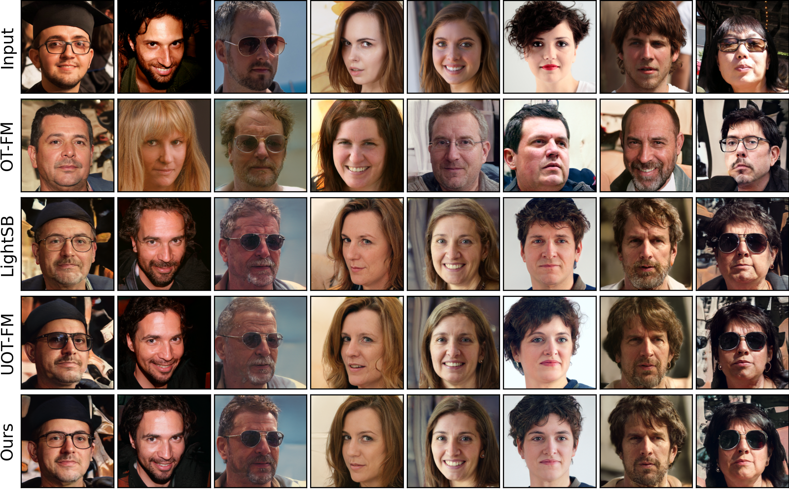
(a) Young $\rightarrow$ Adult

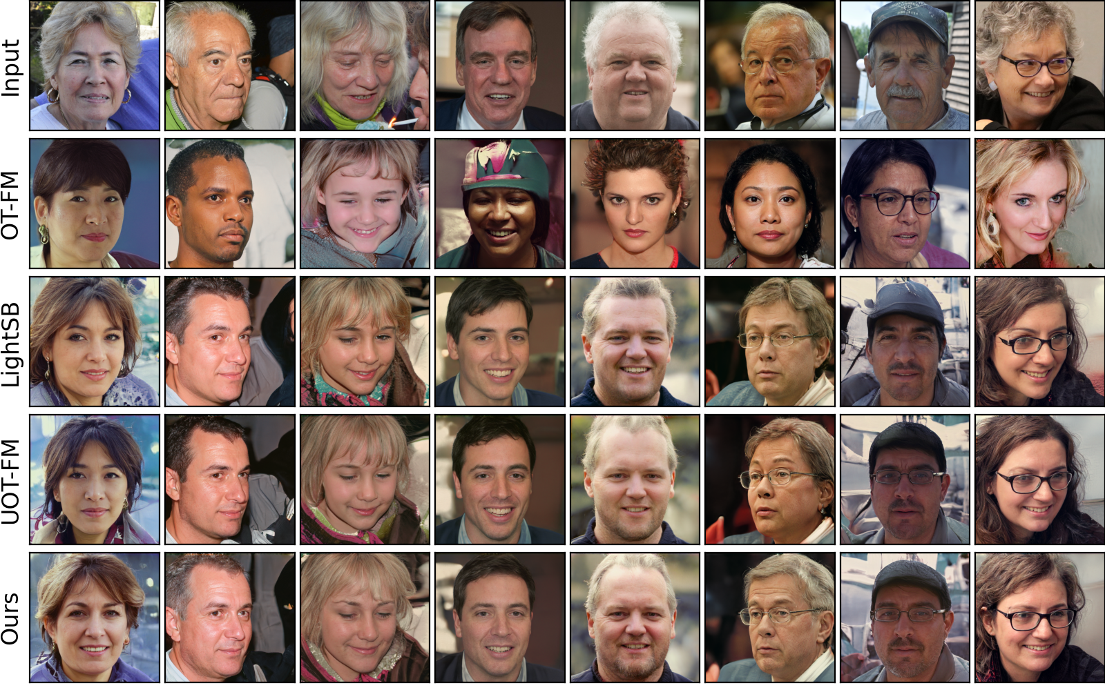
(b) Adult $\rightarrow$ Young

Figure 3: Comparison of solvers, Adult$\leftrightarrow$Young translation.

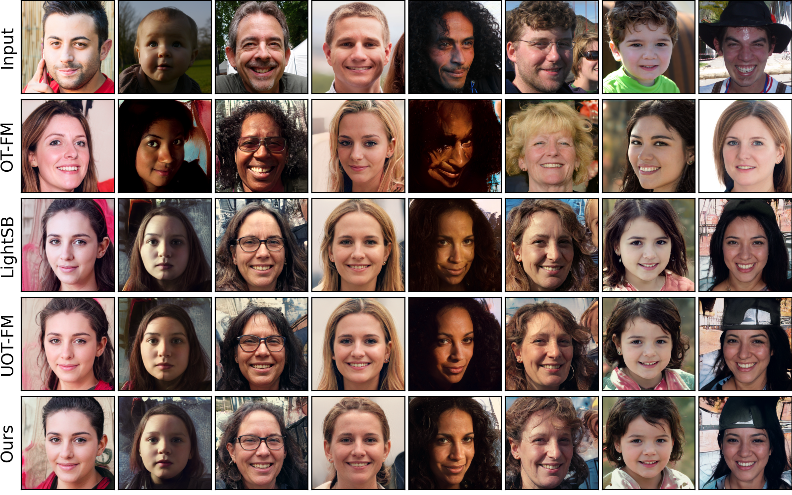
(a) Man $\rightarrow$ Woman

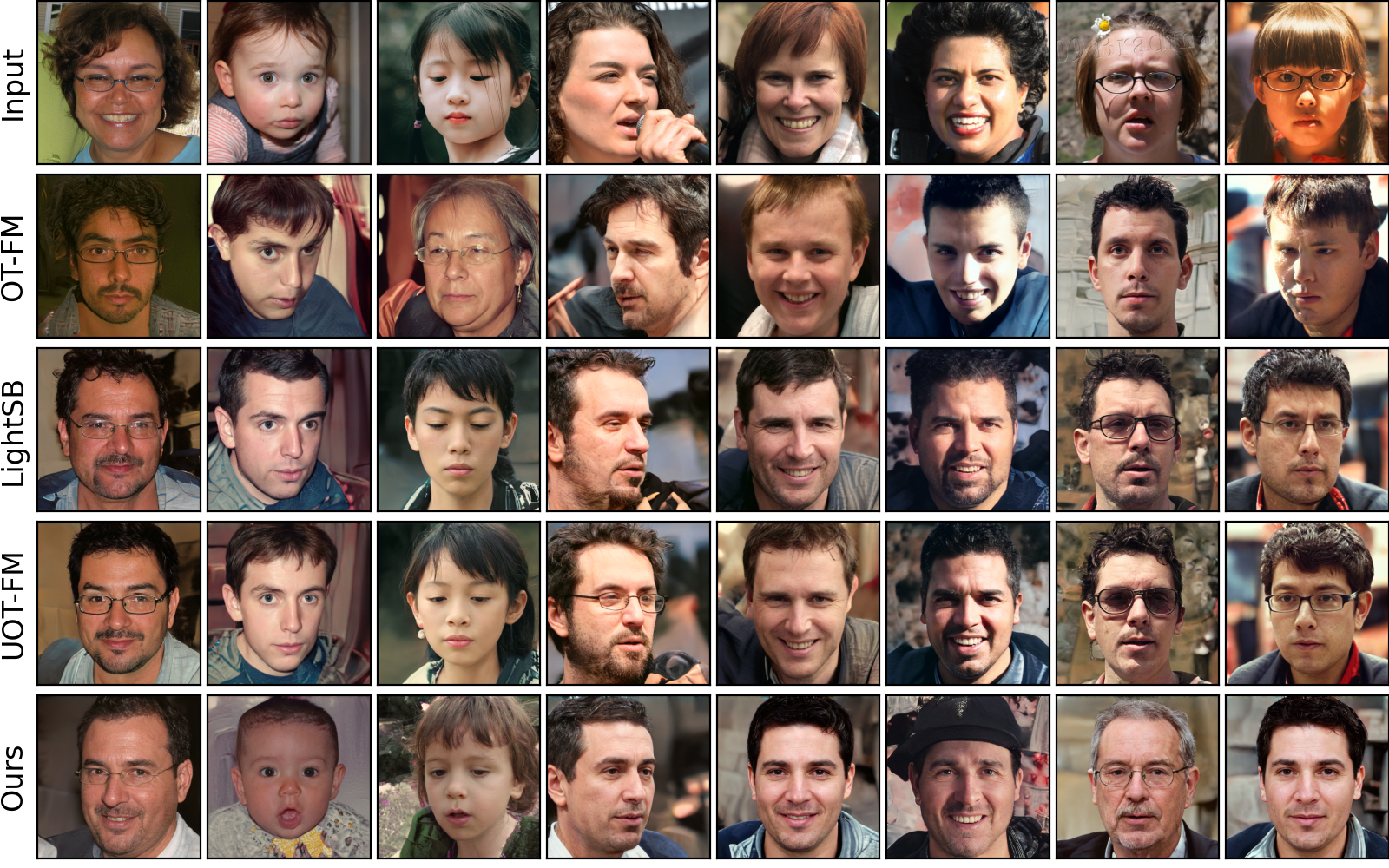
(b) Woman $\rightarrow$ Man

Figure 4: Comparison of solvers, Woman$\leftrightarrow$Man translation.

References

- Arjovsky et al. (2017) Arjovsky, M., Chintala, S., and Bottou, L. Wasserstein generative adversarial networks. In International conference on machine learning, pp. 214–223. PMLR, 2017.
- Asadulaev et al. (2024) Asadulaev, A., Korotin, A., Egiazarian, V., and Burnaev, E. Neural optimal transport with general cost functionals. In The Twelfth International Conference on Learning Representations, 2024.
- Balaji et al. (2020) Balaji, Y., Chellappa, R., and Feizi, S. Robust optimal transport with applications in generative modeling and domain adaptation. Advances in Neural Information Processing Systems, 33:12934–12944, 2020.
- Chapel et al. (2021) Chapel, L., Flamary, R., Wu, H., Févotte, C., and Gasso, G. Unbalanced optimal transport through non-negative penalized linear regression. Advances in Neural Information Processing Systems, 34:23270–23282, 2021.
- Chen et al. (2021) Chen, T., Liu, G.-H., and Theodorou, E. Likelihood training of schrödinger bridge using forward-backward sdes theory. In International Conference on Learning Representations, 2021.
- Chizat (2017) Chizat, L. Unbalanced optimal transport: Models, numerical methods, applications. PhD thesis, Université Paris sciences et lettres, 2017.
- Choi et al. (2023) Choi, J., Choi, J., and Kang, M. Generative modeling through the semi-dual formulation of unbalanced optimal transport. arXiv preprint arXiv:2305.14777, 2023.
- Cuturi (2013) Cuturi, M. Sinkhorn distances: Lightspeed computation of optimal transport. In Advances in neural information processing systems, pp. 2292–2300, 2013.
- Daniels et al. (2021) Daniels, M., Maunu, T., and Hand, P. Score-based generative neural networks for large-scale optimal transport. Advances in neural information processing systems, 34:12955–12965, 2021.
- Dao et al. (2023) Dao, Q., Ta, B., Pham, T., and Tran, A. Robust diffusion gan using semi-unbalanced optimal transport. arXiv preprint arXiv:2311.17101, 2023.
- De Bortoli et al. (2021) De Bortoli, V., Thornton, J., Heng, J., and Doucet, A. Diffusion schrödinger bridge with applications to score-based generative modeling. Advances in Neural Information Processing Systems, 34:17695–17709, 2021.
- Deb et al. (2021) Deb, N., Ghosal, P., and Sen, B. Rates of estimation of optimal transport maps using plug-in estimators via barycentric projections. Advances in Neural Information Processing Systems, 34:29736–29753, 2021.
- Dvurechenskii et al. (2018) Dvurechenskii, P., Dvinskikh, D., Gasnikov, A., Uribe, C., and Nedich, A. Decentralize and randomize: Faster algorithm for Wasserstein barycenters. In Advances in Neural Information Processing Systems, pp. 10760–10770, 2018.
- Eyring et al. (2024) Eyring, L., Klein, D., Uscidda, T., Palla, G., Kilbertus, N., Akata, Z., and Theis, F. Unbalancedness in neural monge maps improves unpaired domain translation. In The Twelfth International Conference on Learning Representations, 2024.
- Fan et al. (2023) Fan, J., Liu, S., Ma, S., Zhou, H.-M., and Chen, Y. Neural monge map estimation and its applications. Transactions on Machine Learning Research, 2023. ISSN 2835-8856. URL https://openreview.net/forum?id=2mZSlQscj3. Featured Certification.
- Fatras et al. (2020) Fatras, K., Zine, Y., Flamary, R., Gribonval, R., and Courty, N. Learning with minibatch wasserstein: asymptotic and gradient properties. In AISTATS 2020-23nd International Conference on Artificial Intelligence and Statistics, volume 108, pp. 1–20, 2020.
- Fatras et al. (2021) Fatras, K., Séjourné, T., Flamary, R., and Courty, N. Unbalanced minibatch optimal transport; applications to domain adaptation. In International Conference on Machine Learning, pp. 3186–3197. PMLR, 2021.
- Flamary et al. (2021) Flamary, R., Courty, N., Gramfort, A., Alaya, M. Z., Boisbunon, A., Chambon, S., Chapel, L., Corenflos, A., Fatras, K., Fournier, N., et al. Pot: Python optimal transport. The Journal of Machine Learning Research, 22(1):3571–3578, 2021.
- Gazdieva et al. (2022) Gazdieva, M., Rout, L., Korotin, A., Kravchenko, A., Filippov, A., and Burnaev, E. An optimal transport perspective on unpaired image super-resolution. arXiv preprint arXiv:2202.01116, 2022.
- Gazdieva et al. (2023) Gazdieva, M., Korotin, A., Selikhanovych, D., and Burnaev, E. Extremal domain translation with neural optimal transport. In Advances in Neural Information Processing Systems, volume 36, 2023.
- Genevay (2019) Genevay, A. Entropy-Regularized Optimal Transport for Machine Learning. Theses, PSL University, March 2019. URL https://theses.hal.science/tel-02319318.
- Genevay et al. (2018) Genevay, A., Peyré, G., and Cuturi, M. Learning generative models with sinkhorn divergences. In International Conference on Artificial Intelligence and Statistics, pp. 1608–1617. PMLR, 2018.
- Gulrajani et al. (2017) Gulrajani, I., Ahmed, F., Arjovsky, M., Dumoulin, V., and Courville, A. C. Improved training of Wasserstein GANs. In Advances in Neural Information Processing Systems, pp. 5767–5777, 2017.
- Gushchin et al. (2023a) Gushchin, N., Kolesov, A., Korotin, A., Vetrov, D., and Burnaev, E. Entropic neural optimal transport via diffusion processes. In Advances in Neural Information Processing Systems, 2023a.
- Gushchin et al. (2023b) Gushchin, N., Kolesov, A., Mokrov, P., Karpikova, P., Spiridonov, A., Burnaev, E., and Korotin, A. Building the bridge of schr" odinger: A continuous entropic optimal transport benchmark. arXiv preprint arXiv:2306.10161, 2023b.
- Hütter & Rigollet (2021) Hütter, J.-C. and Rigollet, P. Minimax estimation of smooth optimal transport maps. 2021.
- Janati et al. (2020) Janati, H., Muzellec, B., Peyré, G., and Cuturi, M. Entropic optimal transport between unbalanced gaussian measures has a closed form. Advances in neural information processing systems, 33:10468–10479, 2020.
- Karras et al. (2019) Karras, T., Laine, S., and Aila, T. A style-based generator architecture for generative adversarial networks. In Proceedings of the IEEE/CVF conference on computer vision and pattern recognition, pp. 4401–4410, 2019.
- Korotin et al. (2021) Korotin, A., Li, L., Genevay, A., Solomon, J. M., Filippov, A., and Burnaev, E. Do neural optimal transport solvers work? a continuous wasserstein-2 benchmark. Advances in Neural Information Processing Systems, 34:14593–14605, 2021.
- Korotin et al. (2022) Korotin, A., Kolesov, A., and Burnaev, E. Kantorovich strikes back! wasserstein gans are not optimal transport? In Thirty-sixth Conference on Neural Information Processing Systems Datasets and Benchmarks Track, 2022.
- Korotin et al. (2024) Korotin, A., Gushchin, N., and Burnaev, E. Light schr" odinger bridge. In The Twelfth International Conference on Learning Representations, 2024.
- Koshizuka & Sato (2022) Koshizuka, T. and Sato, I. Neural lagrangian schr"o dinger bridge: Diffusion modeling for population dynamics. In The Eleventh International Conference on Learning Representations, 2022.
- Liero et al. (2018) Liero, M., Mielke, A., and Savaré, G. Optimal entropy-transport problems and a new hellinger–kantorovich distance between positive measures. Inventiones mathematicae, 211(3):969–1117, 2018.
- Lipman et al. (2022) Lipman, Y., Chen, R. T., Ben-Hamu, H., Nickel, M., and Le, M. Flow matching for generative modeling. arXiv preprint arXiv:2210.02747, 2022.
- Lübeck et al. (2022) Lübeck, F., Bunne, C., Gut, G., del Castillo, J. S., Pelkmans, L., and Alvarez-Melis, D. Neural unbalanced optimal transport via cycle-consistent semi-couplings. arXiv preprint arXiv:2209.15621, 2022.
- Lucic et al. (2018) Lucic, M., Kurach, K., Michalski, M., Gelly, S., and Bousquet, O. Are GANs created equal? a large-scale study. In Advances in neural information processing systems, pp. 700–709, 2018.
- Makkuva et al. (2020) Makkuva, A., Taghvaei, A., Oh, S., and Lee, J. Optimal transport mapping via input convex neural networks. In International Conference on Machine Learning, pp. 6672–6681. PMLR, 2020.
- Manole et al. (2021) Manole, T., Balakrishnan, S., Niles-Weed, J., and Wasserman, L. Plugin estimation of smooth optimal transport maps. arXiv preprint arXiv:2107.12364, 2021.
- Mokrov et al. (2024) Mokrov, P., Korotin, A., and Burnaev, E. Energy-guided entropic neural optimal transport. In The Twelfth International Conference on Learning Representations, 2024.
- Nguyen et al. (2022) Nguyen, Q. M., Nguyen, H. H., Zhou, Y., and Nguyen, L. M. On unbalanced optimal transport: Gradient methods, sparsity and approximation error. arXiv preprint arXiv:2202.03618, 2022.
- Peyré et al. (2019) Peyré, G., Cuturi, M., et al. Computational optimal transport. Foundations and Trends® in Machine Learning, 11(5-6):355–607, 2019.
- Pham et al. (2020) Pham, K., Le, K., Ho, N., Pham, T., and Bui, H. On unbalanced optimal transport: An analysis of sinkhorn algorithm. In International Conference on Machine Learning, pp. 7673–7682. PMLR, 2020.
- Pidhorskyi et al. (2020) Pidhorskyi, S., Adjeroh, D. A., and Doretto, G. Adversarial latent autoencoders. In Proceedings of the IEEE/CVF Conference on Computer Vision and Pattern Recognition, pp. 14104–14113, 2020.
- Pooladian & Niles-Weed (2021) Pooladian, A.-A. and Niles-Weed, J. Entropic estimation of optimal transport maps. arXiv preprint arXiv:2109.12004, 2021.
- Rigollet & Stromme (2022) Rigollet, P. and Stromme, A. J. On the sample complexity of entropic optimal transport. arXiv preprint arXiv:2206.13472, 2022.
- Rout et al. (2022) Rout, L., Korotin, A., and Burnaev, E. Generative modeling with optimal transport maps. In International Conference on Learning Representations, 2022.
- Seguy et al. (2018) Seguy, V., Damodaran, B. B., Flamary, R., Courty, N., Rolet, A., and Blondel, M. Large scale optimal transport and mapping estimation. In International Conference on Learning Representations, 2018.
- Séjourné et al. (2022) Séjourné, T., Peyré, G., and Vialard, F.-X. Unbalanced optimal transport, from theory to numerics. arXiv preprint arXiv:2211.08775, 2022.
- Tong et al. (2020) Tong, A., Huang, J., Wolf, G., Van Dijk, D., and Krishnaswamy, S. Trajectorynet: A dynamic optimal transport network for modeling cellular dynamics. In International conference on machine learning, pp. 9526–9536. PMLR, 2020.
- Vargas et al. (2021) Vargas, F., Thodoroff, P., Lamacraft, A., and Lawrence, N. Solving schrödinger bridges via maximum likelihood. Entropy, 23(9):1134, 2021.
- Wang et al. (2021) Wang, G., Jiao, Y., Xu, Q., Wang, Y., and Yang, C. Deep generative learning via schrödinger bridge. In International Conference on Machine Learning, pp. 10794–10804. PMLR, 2021.
- Xie et al. (2022) Xie, Y., Luo, Y., and Huo, X. An accelerated stochastic algorithm for solving the optimal transport problem. arXiv preprint arXiv:2203.00813, 2022.
- Yang & Uhler (2018) Yang, K. D. and Uhler, C. Scalable unbalanced optimal transport using generative adversarial networks. In International Conference on Learning Representations, 2018.
- Zhu et al. (2017) Zhu, J.-Y., Zhang, R., Pathak, D., Darrell, T., Efros, A. A., Wang, O., and Shechtman, E. Toward multimodal image-to-image translation. Advances in neural information processing systems, 30, 2017.