Parameter estimation of stochastic SIR model driven by small Lévy noises with time-dependent periodic transmission

Abstract

We investigate the parameter estimation and forecasting of two forms of the stochastic SIR model driven by small Lévy noises. We accomplish this by utilizing least squares estimators. We include simulation studies of both forms using the method of projected gradient descent to aid in the parameter estimation.

MSC: 62M05; 92D30; 62F12

Keywords: Unified stochastic SIR model, parameter estimation, least squares method, time-dependency, periodic transmission, Lévy noise.

1 Introduction

Interest in epidemiological models has increased in the previous decade especially with random noises added to the models. The classical Susceptible-Infected-Recovered (SIR) model, which was introduced by Kermack and McKendrick [23] nearly a century ago is defined as:

$$\begin{cases}\frac{dX_{t}}{dt}=-\beta X_{t}Y_{t},\\ \frac{dY_{t}}{dt}=\left(\beta X_{t}-\gamma\right)Y_{t},\\ \frac{dZ_{t}}{dt}=\gamma Y_{t},\end{cases}$$

where $\beta$ is the transmission rate and $\gamma$ the recovery rate. Additionally, demographics may be introduced to include birth rate $\Lambda$ and mortality rate $\mu$ as:

$$\begin{cases}\frac{dX_{t}}{dt}=\Lambda-\mu X_{t}-\beta X_{t}Y_{t},\\ \frac{dY_{t}}{dt}=\left[\beta X_{t}-(\mu+\gamma)\right]Y_{t},\\ \frac{dZ_{t}}{dt}=\gamma Y_{t}-\mu Z_{t}.\end{cases}$$

These deterministic models have been put into various stochastic frameworks that make the situation more realistic (cf. e.g., [40], [16], [21], [2], [5], [45], [47], [48], [11], [28], [29] and [12]). More recently, the unified stochastic SIR (USSIR) model was introduced by the authors in [9]. The USSIR model is defined as

$$\begin{cases}\begin{split}&dX_{t}=\ b_{1}(t,X_{t},Y_{t},Z_{t})dt+\sum\limits_{j=1}^{r}\sigma_{1j}(t,X_{t},Y_{t},Z_{t})dB_{t}^{(j)}\\ &\indent\indent+\int_{\left\{\lvert u\rvert\leq 1\right\}}H_{1}(t,X_{t-},Y_{t-},Z_{t-},u)\tilde{N}(dt,du)+\int_{\left\{\lvert u\rvert>1\right\}}G_{1}(t,X_{t-},Y_{t-},Z_{t-},u)N(dt,du),\end{split}\\ \begin{split}&dY_{t}=\ b_{2}(t,X_{t},Y_{t},Z_{t})dt+\sum\limits_{j=1}^{r}\sigma_{2j}(t,X_{t},Y_{t},Z_{t})dB_{t}^{(j)}\\ &\indent\indent+\int_{\left\{\lvert u\rvert\leq 1\right\}}H_{2}(t,X_{t-},Y_{t-},Z_{t-},u)\tilde{N}(dt,du)+\int_{\left\{\lvert u\rvert>1\right\}}G_{2}(t,X_{t-},Y_{t-},Z_{t-},u)N(dt,du),\end{split}\\ \begin{split}&dZ_{t}=\ b_{3}(t,X_{t},Y_{t},Z_{t})dt+\sum\limits_{j=1}^{r}\sigma_{3j}(t,X_{t},Y_{t},Z_{t})dB_{t}^{(j)}\\ &\indent\indent+\int_{\left\{\lvert u\rvert\leq 1\right\}}H_{3}(t,X_{t-},Y_{t-},Z_{t-},u)\tilde{N}(dt,du)+\int_{\left\{\lvert u\rvert>1\right\}}G_{3}(t,X_{t-},Y_{t-},Z_{t-},u)N(dt,du).\end{split}\\ \end{cases}$$ (1.1)

Hereafter, $\mathbb{R}_{+}$ denotes the set of all positive real numbers, $(B_{t})_{t\geq 0}=(B^{(1)}_{t},\dots,B^{(r)}_{t})_{t\geq 0}$ is a standard $r$-dimensional Brownian motion, $N$ is a Poisson random measure on $\mathbb{R}_{+}\times(\mathbb{R}^{l}\backslash\{0\})$ with intensity measure $\mu$ satisfying $\int_{\mathbb{R}^{l}\backslash\{0\}}(1\wedge|u|^{2})\mu(du)<\infty$ and $\tilde{N}(dt,du)=N(dt,du)-\mu(du)dt$, $(B_{t})_{t\geq 0}$ and $N$ are independent, $b_{i},\sigma_{ij}:[0,\infty)\times\mathbb{R}^{3}_{+}\mapsto\mathbb{R}$, $H_{i},G_{i}:[0,\infty)\times\mathbb{R}^{3}_{+}\times(\mathbb{R}^{l}\backslash\{0\})\mapsto\mathbb{R}$, $i=1,2,3,\ j=1,2,\ldots,n$, are measurable functions.

The goal of this paper is to accomplish parameter estimation of a periodic transmission function present in a stochastic SIR model, e.g., the USSIR model (1.1). It is a natural question to ask if transmission of a disease is periodic. Understanding this periodicity greatly aids in ability to predict possible outcomes. A potential application is in the study of periodicity in the COVID-19 pandemic, as well as future pandemics. The stochastic model chosen has driving noise of the Lévy variety subjected to a small coefficient $\varepsilon$. In our study, we focus not only on estimating unknown parameters and forecasting future behaviour but also the asymptotics of our estimators. Given the complexity of the model, we use optimization techniques to iteratively solve for approximations to the estimators.

In recent times, the study of parameter estimation in stochastic epidemiological models has been gaining momentum, but there is still much work that needs to be completed. Notable works are available in the literature, see e.g., [13], [7], [27], [33], [35], [46], [17], [26], [34], [20], [43], [1], [6], [10], [14], [36], [4] and [25]. For our studies, the focus is primarily the periodicity of transmission of disease. It is worth noting that we assume no prior knowledge on the explicit form of the random noise. Additionally, the periodicity we seek to estimate is not assumed to be tied to specific time periods such as days, weeks or months; rather, whatever the observed time period may be is what determines the time scale in which the periodicity occurs.

In addition to papers on parameter estimation of epidemiological models, there is a growing number of works which consider the more general setting of parameter estimation for stochastic differential equations (SDEs) with small Lévy noises regardless of specific applications (cf. e.g., [22], [39], [41], [44], [15], [38], [30], [8], [31] and [24]). The methodology we use in the paper is directly inspired by the results of Long et al. in [30] and [31]. More specifically, we use the least-squares method, similarly to what has been completed in [30] and [31], to estimate a true parameter $\theta_{0}$ of a discretely observed stochastic process. We introduce a contrast function from which we are able to derive the least-squares estimators (LSEs) and obtain results on the consistency and limiting distributions of the estimators.

Consider a stochastic process $(S^{\varepsilon}_{t})_{t\geq 0}$ which satisfies the SDE:

$$dS^{\varepsilon}_{t} = b(t,S^{\varepsilon}_{t},\theta)dt$$

$$+\varepsilon\left\{\sigma(t,S^{\varepsilon}_{t})dB_{t}+{\int_{\{|u|\leq 1\}}}H(t,S^{\varepsilon}_{t-},u)\widetilde{N}(dt,du)+{\int_{\{|u|>1\}}}G(t,S^{\varepsilon}_{t-},u)N(dt,du)\right\},$$

where $0<\varepsilon<1$, $t\in[0,1]$, $S^{\varepsilon}_{0}=s\in\mathbb{R}^{d}$, $\theta\in\overline{\Theta}$, the closure of an open convex bounded subset $\Theta$ of $\mathbb{R}^{p}$, $b(\cdot,\cdot,\cdot):[0,\infty)\times\mathbb{R}^{d}\times\Theta\to\mathbb{R}^{d}$, $\sigma(\cdot,\cdot):[0,\infty)\times\mathbb{R}^{d}\to\mathbb{R}^{d\times r}$, $H(\cdot,\cdot,\cdot)$, $G(\cdot,\cdot,\cdot):[0,\infty)\times\mathbb{R}^{d}\times(\mathbb{R}^{l}\backslash\{0\})\to\mathbb{R}^{d}$ are Borel measurable functions. Suppose $(S^{\varepsilon}_{t})_{t\geq 0}$ is observed at regularly spaced time points $\{t_{k}=\frac{k}{n}$, $k=1,2,\dots,n\}$. Define the contrast function

$$\Psi_{n,\varepsilon}(\theta)=\sum_{k=1}^{n}\varepsilon^{-2}nP_{k}^{*}(\theta)P_{k}(\theta),$$

where

$$P_{k}(\theta)=S^{\varepsilon}_{t_{k}}-S^{\varepsilon}_{t_{k-1}}-\frac{1}{n}b(t_{k-1},S^{\varepsilon}_{t_{k-1}},\theta).$$

Let $\hat{\theta}_{n,\varepsilon}$ be a minimum contrast estimator, i.e., a random variable satisfying

$$\hat{\theta}_{n,\varepsilon}:={\rm arg\,min}_{\theta\in\Theta}\Psi_{n,\varepsilon}(\theta).$$

As we will see for the USSIR model, finding a closed form for the LSE $\hat{\theta}_{n,\varepsilon}$ can be quite difficult, thus we look for suitable approximations $\hat{\theta}_{n,\varepsilon}^{*}$ of $\hat{\theta}_{n,\varepsilon}$. In the vernacular for optimization, we may refer to our contrast function $\Psi_{n,\varepsilon}(\theta)$ as an objective function. Given an objective function that one wishes to minimize for estimation purposes a commonly utilized method is gradient descent (GD) (cf. [3, Section 8.1] for more information). More explicitly, given a convex function $f$ without constraints such that one wishes to solve

$$\arg\min_{x}f(x),$$

the method of GD minimizes by making use of the update rule

$$x^{(k+1)}=x^{(k)}-\eta\nabla f(x^{(k)})$$

for some initial value $x^{(0)}$ and learning rate $\eta>0$. With the presence of constraints, GD is still applicable in the form of projected gradient descent (PGD) (cf. [3, Section 10.2]). That is, given a convex function $f$ and a constraint set $\mathcal{C}$, one would use a similar update rule which can be stated as

$$y^{(k+1)}=x^{(k)}-\eta\nabla f(x^{(k)});\ \ x^{(k+1)}=\arg\min_{x\in\mathcal{C}}|y^{(k+1)}-x|.$$

The remainder of this paper is organized as follows. Section 2 gives the theoretical results on LSEs for time-dependent SDEs driven by small Lévy noises with applications to the USSIR model (1.1). Sections 3 and 4 cover simulation studies of SIR models for population proportions and population numbers, respectively. Section 5 is a closing discussion.

2 Least-squares estimators for time-dependent SDEs driven by small Lévy noises

2.1 General time-dependent SDEs driven by small Lévy noises

In this subsection, we investigate LSEs for discretely observed stochastic processes driven by small Lévy noises. The results presented here generalize the results of Long et al. in [30] and [31]. Our contributions are the generalization to a time-dependent jump-diffusion model, which is more general to include different (singular and non-singular) coefficient functions for the Brownian motion, small jump and large jump portions. Also noteworthy, is we use a contrast function which is different from that in [31]; however, we also provide a result which uses the same contrast function as that in [31] when the coefficient functions are equal and non-singular.

The primary focus of this paper is the parameter estimation for a stochastic SIR model; hence, proofs for the following results are omitted. We wish to note that the proofs required to establish our results are obtained without essential difficulties and follow the same pattern as that of [30] and [31].

Suppose that $(S^{\varepsilon}_{t})_{t\geq 0}$ satisfies the SDE (1). Consider an underlying deterministic (ordinary) differential equation denoted as

$$dS^{0}_{t}=b(t,S_{t}^{0},\theta_{0}),\ t\in[0,1],\ S^{0}_{0}=s,$$

where $\theta_{0}$ is the true value of the drift parameter. We take the following assumptions which are modifications of those given in [31].

(A1) For all $\varepsilon>0$, the SDE (1) admits a unique strong solution $S^{\varepsilon}$ (cf. [18, Theorem 2.2] for concrete sufficient conditions).

(A2) There exist $K>0$ and $\eta,\xi\in{\mathcal{B}}_{+}(\mathbb{R}^{l})$ such that for any $t\in[0,1]$, $x,y\in\mathbb{R}^{d}$, $u\in\mathbb{R}^{l}\backslash\{0\}$ and $\theta\in\overline{\Theta}$,

$$|b(t,x,\theta)-b(t,y,\theta)|\leq K|x-y|,\ \ \ \ \int_{|v|\leq 1}\eta^{2}(v)\mu(dv)<\infty,$$

$$|b(t,x,\theta)|+|\sigma(t,x)|+\frac{1_{\{|u|\leq 1\}}|H(t,x,u)|}{\eta(u)}+\frac{1_{\{|u|>1\}}|G(t,x,u)|}{\xi(u)}\leq K(1+|x|).$$

(A3) $b(\cdot,\cdot,\cdot)\in C_{\uparrow}^{1,1,3}([0,1]\times\mathbb{R}^{d}\times\Theta;\mathbb{R}^{d})$, i.e., $b$ is continuously differentiable and thrice continuously differentiable in $t,x$ and $\theta$, respectively, and there exist constants $C,\lambda>0$ such that

$$\sup_{t\in[0,1]}\sup_{\theta\in\Theta}\lvert\partial^{\nu_{3}}_{\theta}\partial^{\nu_{2}}_{x}\partial^{\nu_{1}}_{t}b(t,x,\theta)\rvert\leq C(1+|x|)^{\lambda},$$

for any multi-indices $\nu_{1},\nu_{2},\nu_{3}$ satisfying

$$0\leq\nu_{1}\leq 1,\ \ 0\leq\sum_{i=1}^{d}\nu_{2}^{(i)}\leq 1,\ \ 0\leq\sum_{j=1}^{p}\nu_{3}^{(j)}\leq 3.$$

(A4) $\theta\neq\theta_{0}\Leftrightarrow\exists t\in[0,1]$ such that $b(t,S_{t}^{0},\theta)\neq b(t,S_{t}^{0},\theta_{0})$.

(A5) $\sigma(\cdot,\cdot)$ is continuous on $[0,1]\times\mathbb{R}^{d}$ and $H(\cdot,\cdot,u)$, $G(\cdot,\cdot,u)$ are continuous on $[0,1]\times\mathbb{R}^{d}$ for any $u\in\mathbb{R}^{l}\backslash\{0\}$.

(A6) $\varepsilon=\varepsilon_{n}\rightarrow 0$ and $n\varepsilon\rightarrow\infty$ as $n\rightarrow\infty$.

We adopt the notation $o_{p}(1)$ which is short for a sequence of random vectors that converges to zero in probability, and the notation $\xrightarrow{P_{\theta_{0}}}$ which is short for convergence in probability under $P_{\theta_{0}}$. By virtue of [42, Theorem 5.7], similar to [30, 31, Theorem 2.1], we can prove the following result on consistency of the LSEs.

Theorem 2.1

Let $\hat{\theta}^{*}_{n,\varepsilon}$ be any sequence of estimators with $\Psi_{n,\varepsilon}(\hat{\theta}^{*}_{n,\varepsilon})\leq\Psi_{n,\varepsilon}(\theta_{0})+o_{p}(1)$. Then, under conditions (A1)-(A4), we have

$$\hat{\theta}^{*}_{n,\varepsilon}\xrightarrow{P_{\theta_{0}}}\theta_{0}\text{ as }\varepsilon\to 0\text{ and }n\to\infty.$$

Define the matrix $I(\theta)=(I^{ij}(\theta))_{1\leq i,j\leq p}$ by

$$I^{ij}(\theta)=\int_{0}^{1}(\partial_{\theta_{i}}b)^{*}(r,S^{0}_{r},\theta)\partial_{\theta_{j}}b(r,S^{0}_{r},\theta)dr.$$

Similar to [30, 31, Theorem 2.2], we can prove the following result on rate of convergence of the LSEs.

Theorem 2.2

Assume that conditions (A1)-(A6) hold and $I(\theta_{0})$ is positive definite. Then,

$$\varepsilon^{-1}(\hat{\theta}_{n,\varepsilon}-\theta_{0}) \xrightarrow{P_{\theta_{0}}} I^{-1}(\theta_{0})\left(\int_{0}^{1}(\partial_{\theta_{i}}b)^{*}(r,S^{0}_{r},\theta)\Bigg{\{}\sigma(r,S^{0}_{r})dB_{r}\right.$$

$$\left.\ \ \ \ +{\int_{\{|u|\leq 1\}}}H(r,S^{0}_{r},u)\widetilde{N}(dr,du)+{\int_{\{|u|>1\}}}G(r,S^{0}_{r},u)N(dr,du)\Bigg{\}}\right)^{*}_{1\leq i\leq p}$$

$\text{ as }\varepsilon\to 0\text{ and }n\to\infty$.

Remark 2.3

Consider the following SDE:

$$dS^{\varepsilon}_{t}=b(t,S^{\varepsilon}_{t},\theta)dt+\varepsilon\sigma(t,S^{\varepsilon}_{t})\left\{dB_{t}+{\int_{\{|u|\leq 1\}}}u\widetilde{N}(dt,du)+{\int_{\{|u|>1\}}}uN(dt,du)\right\}.$$

In the event the diffusion matrix $\sigma\sigma^{*}$ is invertible, we may use the following contrast function from Long et al. [31]:

$$\Psi_{n,\varepsilon}(\theta)=\bigg{(}\sum_{k=1}^{n}\varepsilon^{-2}nP_{k}^{*}(\theta)\Lambda_{k-1}^{-1}P_{k}(\theta)\bigg{)}1_{\{D>0\}},$$ (2.1)

where

$$P_{k}(\theta)=S^{\varepsilon}_{t_{k}}-S^{\varepsilon}_{t_{k-1}}-\frac{1}{n}b(t_{k-1},S^{\varepsilon}_{t_{k-1}},\theta),\ \ \Lambda_{k-1}=[\sigma\sigma^{*}](t_{k-1},S_{t_{k-1}}),\ \ D=\inf_{k=0,\ldots,n-1}\det\Lambda_{k}.$$

Define the matrix $I(\theta)=(I^{ij}(\theta))_{1\leq i,j\leq p}$ by

$$I^{ij}(\theta)=\int_{0}^{1}(\partial_{\theta_{i}}b)^{*}(r,S^{0}_{r},\theta)[\sigma\sigma^{*}]^{-1}(r,S^{0}_{r})\partial_{\theta_{j}}b(r,S^{0}_{r},\theta)dr.$$ (2.2)

We make the following additional assumption.

(A7) There exists an open convex subset $\mathcal{U}\subset\mathbb{R}^{d}$ such that $X_{t}^{0}\in\mathcal{U}$ for all $t\in[0,1]$, $\sigma$ is smooth on $[0,1]\times\mathcal{U}$, and $\sigma\sigma^{*}$ is invertible on $[0,1]\times\mathcal{U}$.

Following the arguments of [30, 31, Theorems 2.1 and 2.2], we can prove the following result.

Corollary 2.4

Assume that conditions (A1)-(A7) hold and $I(\theta_{0})$ defined by (2.2) is positive definite. Then, the assertions of Theorems 2.1 and 2.2 hold for the LSE derived from the contrast function (2.1).

2.2 Application to USSIR model with periodic transmission

Setting $d=3$, we use equation (1) to write the USSIR model as

$$\begin{bmatrix}dX_{t}^{\varepsilon}\\ dY_{t}^{\varepsilon}\\ dZ_{t}^{\varepsilon}\\ \end{bmatrix} = \begin{bmatrix}b_{1}(t,X_{t}^{\varepsilon},Y_{t}^{\varepsilon},Z_{t}^{\varepsilon},\theta)\\ b_{2}(t,X_{t}^{\varepsilon},Y_{t}^{\varepsilon},Z_{t}^{\varepsilon},\theta)\\ b_{3}(t,X_{t}^{\varepsilon},Y_{t}^{\varepsilon},Z_{t}^{\varepsilon},\theta)\end{bmatrix}dt+\varepsilon\bigg{\{}\sigma(t,X_{t}^{\varepsilon},Y_{t}^{\varepsilon},Z_{t}^{\varepsilon})dB_{t}$$

$$\ \ \ \ +{\int_{\{|u|\leq 1\}}}H(t,X^{\varepsilon}_{t-},Y^{\varepsilon}_{t-},Z^{\varepsilon}_{t-},u)\widetilde{N}(dt,du)$$

$$\ \ \ \ +{\int_{\{|u|>1\}}}G(t,X^{\varepsilon}_{t-},Y^{\varepsilon}_{t-},Z^{\varepsilon}_{t-},u)N(dt,du)\bigg{\}},$$

such that all previously stated assumptions hold. Above in equation (2.2), the drift function $b=(b_{1},b_{2},b_{3})$ is given in more general terms but in the subsequent sections explicit instances will be given. Moreover, at the centre of our focus in this paper is the presence of a periodic transmission function. Since any well-behaved periodic function may be approximated using a Fourier series, we consider the drift function to contain a periodic transmission function of the form

$$\beta(t)=\alpha_{0}+\sum_{k=1}^{K}\alpha_{1,k}\cos\left(\frac{2\pi kt}{\theta}\right)+\alpha_{2,k}\sin\left(\frac{2\pi kt}{\theta}\right),$$ (2.4)

where $\theta,\alpha_{0},\alpha_{1,k},\alpha_{2,k}>0,1\leq k\leq K$. This leads to the contrast function being denoted by $\Psi_{n,\varepsilon}(\theta,\alpha_{0},(\alpha_{1,k},\alpha_{2,k})_{k=1}^{K})$ so that our parameters are represented by the vector $(\theta,\alpha_{0},(\alpha_{1,k},\alpha_{2,k})_{k=1}^{K})$ $\in\mathbb{R}_{+}^{2K+2}$. Moreover, assume that $\theta\in[0,1]$, a natural assumption to make given the estimation happens from time $t=0$ to $t=1$. The contrast function $\Psi_{n,\varepsilon}(\theta,\alpha_{0},(\alpha_{1,k},\alpha_{2,k})_{k=1}^{K})$ is not globally convex; however, for a fixed $\theta$, it becomes convex in the remaining parameters. Hence, we introduce the following algorithm:

Algorithm 1   Linear-Search Gradient-Descent (LS-GD)

For $i$ in $1$ to $M$,
StepFix a test value of $\theta$: $\theta_{i}\in\left(\frac{i-1}{M},\frac{i}{M}\right)$;
StepSet the initial value $(\alpha_{0}^{(0)},(\alpha_{1,k}^{(0)},\alpha_{2,k}^{(0)})_{k=1}^{K})$;
StepRun Gradient Descent on the function $\Psi_{n,\varepsilon}(\theta_{i},\alpha_{0},(\alpha_{1,k},\alpha_{2,k})_{k=1}^{K})$ with update rule
Step$(\alpha_{0}^{(l)},(\alpha_{1,k}^{(l+1)},\alpha_{2,k}^{(l+1)})_{k=1}^{K})=(\alpha_{0}^{(l)},(\alpha_{1,k}^{(l)},\alpha_{2,k}^{(l)})_{k=1}^{K})-\eta\nabla_{\{\alpha_{0},(\alpha_{1,k},\alpha_{2,k})_{k=1}^{K}\}}\Psi_{n,\varepsilon}(\theta_{i},\alpha_{0}^{(l)},(\alpha_{1,k}^{(l)},\alpha_{2,k}^{(l)})_{k=1}^{K})$;
StepStore $\Psi^{*}_{i}:=\arg\min\limits_{\{\alpha_{0},(\alpha_{1,k},\alpha_{2,k})_{k=1}^{K}\}}\Psi_{n,\varepsilon}(\theta_{i},\alpha_{0},(\alpha_{1,k},\alpha_{2,k})_{k=1}^{K})$.
End
Return $\min_{i\in\{1,\ldots,M\}}\Psi^{*}_{i}$.

The returned value $\min_{i\in\{1,\ldots,M\}}\Psi^{*}_{i}$ will be the approximation $(\theta^{*},\alpha_{0}^{*},(\alpha_{1,k}^{*},\alpha_{2,k}^{*})_{k=1}^{K})$ of the LSE $(\hat{\theta},\hat{\alpha}_{0},(\hat{\alpha}_{1,k},\hat{\alpha}_{2,k})_{k=1}^{K})$ we seek.

Remark 2.5

The above algorithm can be modified for PGD, which we do indeed use as will be seen in the simulation studies.

For the remainder, we take $K=1$, that is we consider the case when $\beta(t)=\alpha_{0}+\alpha_{1}\cos(2\pi t/\theta)+\alpha_{2}\sin(2\pi t/\theta)$. Choosing $K>1$ does not contribute any more insights. Additionally, choosing $K>1$ would be more computationally expensive to evaluate in our simulation studies.

Recall that our primary goal is estimation of the unknown period $\theta$ and the coefficients $(\alpha_{0},\alpha_{1},\alpha_{2})$ of the periodic transmission function $\beta(t)$. The presence of noise makes for a more realistic model; moreover, we make no assumptions about the exact forms of the noise coefficient functions $\sigma,H,G$.

3 Simulation study of SIR model for population proportions

For this study, the unknown parameters are represented by the vector $\left(\theta,\alpha_{0},\alpha_{1},\alpha_{2}\right)\in\mathbb{R}^{4}_{+}$ and our objective function is denoted $\Psi_{n,\varepsilon}\left(\theta,\alpha_{0},\alpha_{1},\alpha_{2}\right)$ where $n$ is the number of observations we have and $\varepsilon\in(0,1)$. For a fixed $\theta$, recall the convexity of $\Psi_{n,\varepsilon}\left(\theta,\alpha_{0},\alpha_{1},\alpha_{2}\right)$ with respect to $(\alpha_{0},\alpha_{1},\alpha_{2})$ one only needs to check the Hessian matrix is positive semi-definite.

For our simulation and numerical estimation results we make use of the Julia programming language. This language is well suited for this application as it was created with the purpose of being a high-level programming language which is scientific computing centric. We use two well maintained Julia packages; namely, DifferentialEquations.jl and Optim.jl (cf. [32] and [37]). More of which is discussed below; however, we want to note the package Optim.jl handles the projection to the constraint set for us; namely, as we are not computing these estimates by hand we are able to reasonably circumvent difficulty presented by projecting to the constraint set. In short, we pass the constraint set $\mathcal{C}$ as an argument to the suitable method from Optim.jl.

Using the Julia programming language, and utilizing the package DifferentialEquations.jl, we are able to generate synthetic data for our testing purposes – we generate the data such that we have $100$ observations. Namely, an Euler-Maruyama discretization of the USSIR model is used from which we take $100$ observations to utilize in the estimation of the unknown parameters. We next construct the contrast function and approximate the LSE by use of the LS-GD algorithm. We accomplish the task of implementing the LS-GD algorithm with the aid of the Julia package Optim.jl. More explicitly, the learning rate $\eta$, present in the update rule in (Algorithm 1), is chosen by a Hager-Zhang line-search algorithm. For a more in-depth exploration, we refer the reader to the Optim.jl documentation in [32] and also to the paper by Hager and Zhang [19].

Noteworthy, is that the contrast function $\Psi_{n,\varepsilon}$ is non-linear in the unknown parameters. This is clear by the definition of $\beta(t)$. Hence, there is inter-play, or dependence of optimal estimators between $\alpha_{i}$ and $\theta$ for $i=1,2$. Moreover, this leads to the interesting results that we are able to estimate two or more unknown parameters which are present in a dependent setting of a multiplicative form.

Remark 3.1

Through some heuristics we arrived at the initial value $(\alpha_{0}^{(0)},\alpha_{1}^{(0)},\alpha_{2}^{(0)})\newline =(0.5,0.31,0.21)$; which is used in all implementations of the LS-GD algorithm for the purposes of this paper. There is nothing particularly significant about this value hence we have no reason to believe it had any impact on our findings.

For choosing the test values of $\theta_{i}$, we chose them such that $\theta_{i}\sim\text{Uniform}(\frac{i-1}{M},\frac{i}{M})$. As the value $M$ increases, it does not make a difference if we individually choose the value or allow it to be randomly assigned within each subinterval.

3.1 Model for population proportions

Consider the following model for population proportions:

$$\begin{bmatrix}dX_{t}\\ dY_{t}\\ dZ_{t}\end{bmatrix}=\begin{bmatrix}-\beta(t)X_{t}Y_{t}\\ \beta(t)X_{t}Y_{t}-\gamma Y_{t}\\ \gamma Y_{t}\end{bmatrix}dt\,+\,\varepsilon\!\begin{bmatrix}-\sigma X_{t-}Y_{t-}Z_{t-}\\ 2\sigma X_{t-}Y_{t-}Z_{t-}\\ -\sigma X_{t-}Y_{t-}Z_{t-}\end{bmatrix}dL_{t},\vspace{1cm}$$ (3.1)

where

$$L_{t}=B_{t}+\displaystyle\int_{0}^{t}\displaystyle\int_{\{|u|>0.1\}}uN(ds,du),$$

and as before,

$$\beta(t)=\alpha_{0}+\alpha_{1}\cos\left(\frac{2\pi t}{\theta}\right)+\alpha_{2}\sin\left(\frac{2\pi t}{\theta}\right),\ \ \ \ \theta\in[0,1],\alpha_{0},\alpha_{1},\alpha_{2}>0,$$

$\gamma,\sigma>0$ are constants, and $N=N_{1}+N_{2}$ such that $N_{1}$, $N_{2}$ are independent Poisson random measures with respective intensity measures $\mu_{1}$ and $\mu_{2}$:

$$\begin{cases}N_{1}\sim\frac{2}{3}\lambda dt\mu_{1}(du)\text{ with }\mu_{1}=\delta(\{-0.1,0.1,0.0\}),\\ N_{2}\sim\frac{1}{3}\lambda dt\mu_{2}(du)\text{ with }\mu_{2}=\delta(\{0.0,-0.1,0.1\}),\end{cases}$$ (3.2)

where $\lambda\sim\text{Uniform}(\{1,2,3,4\})$.

By [9, Theorem 2.1], the SDE (3.1) has a unique strong solution taking values in the set $\Delta=\{(x,y,z)\in\mathbb{R}^{3}_{+}:x+y+z=1\}$. It is easy to verify that all assumptions of Theorems 2.1 and 2.2 hold. We use the following contrast function:

$$\Psi_{\varepsilon,n}(\theta,\alpha_{0},\alpha_{1},\alpha_{2})=100\varepsilon^{-2}\left(\sum_{k=1}^{100}P_{k}^{*}(\theta,\alpha_{0},\alpha_{1},\alpha_{2})P_{k}(\theta,\alpha_{0},\alpha_{1},\alpha_{2})\right),$$

where

$$P_{k}(\theta,\alpha_{0},\alpha_{1},\alpha_{2})=\begin{bmatrix}X_{t_{k}}-X_{t_{k-1}}-\frac{1}{100}\left[-\beta({t_{k-1}})X_{t_{k-1}}Y_{t_{k-1}}\right]\\ Y_{t_{k}}-Y_{t_{k-1}}-\frac{1}{100}\left[\beta({t_{k-1}})X_{t_{k-1}}Y_{t_{k-1}}-\gamma Y_{t_{k-1}}\right]\\ Z_{t_{k}}-Z_{t_{k-1}}-\frac{1}{100}\gamma Y_{t_{k-1}}\end{bmatrix}.$$

.

3.2 Parameter estimation

We generate the synthetic data $10000$ times and randomly chose $1000$ such data sets to perform estimation upon. Set $\gamma=0.07142$, $\sigma=0.5$ and $(X_{0},Y_{0},Z_{0})=(0.84,0.07,0.11)$. For the unknown parameters, the true values for use in generating the synthetic data are randomly decided upon as follows

$$\theta\sim\text{Uniform}(0,1),\ \ \alpha_{0}\sim\text{Uniform}(0.1,0.8),\ \ \alpha_{1},\alpha_{2}\sim\text{Uniform}\left(0,\frac{\alpha_{0}}{\sqrt{2}}\right).$$ (3.3)

It is noteworthy that although the distributions of $\alpha_{1},\alpha_{2}$ are dependent on the distribution of $\alpha_{0}$, their specific values are not. The reasoning for this dependency is we require $\beta(t)\geq 0$. Also note that for each generation of synthetic data, the jump parameter $\lambda$ is randomly chosen as described in (3.2).

The subsequent plots and table contain our findings and the metric we use to test our methodology is

$$MAE=\sum_{i=1}^{1000}\frac{\lvert y_{i}-\hat{y_{i}}\rvert}{1000},$$

where $y_{i}$ is the true value and $\hat{y_{i}}$ is the estimated value for $\theta,\alpha_{0},\alpha_{1},\alpha_{2}$.

$\varepsilon$	Parameter	MAE
$0.3$
	$\theta$	0.0980807
	$\alpha_{0}$	0.021481
	$\alpha_{1}$	0.055916
	$\alpha_{2}$	0.058691
$0.1$
	$\theta$	0.0416584
	$\alpha_{0}$	0.009259
	$\alpha_{1}$	0.034566
	$\alpha_{2}$	0.0368507
$0.01$
	$\theta$	0.021081
	$\alpha_{0}$	0.005788
	$\alpha_{1}$	0.033258
	$\alpha_{2}$	0.0333328
$0.001$
	$\theta$	0.0205791
	$\alpha_{0}$	0.005601
	$\alpha_{1}$	0.03208
	$\alpha_{2}$	0.03183

Table 1: Metrics of estimated parameters for $1000$ estimations of $100$ observations using $200$ values of $\hat{\theta}$.

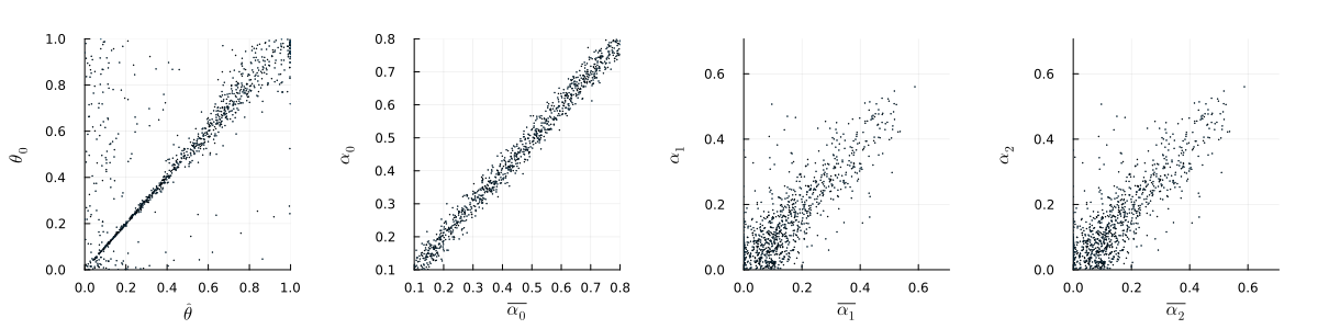
Figure 1: Estimates against true values for $1000$ estimations of $100$ observations using $200$ values of $\hat{\theta}$ while $\varepsilon=0.3$.

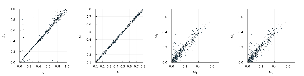
Figure 2: Estimates against true values for $1000$ estimations of $100$ observations using $200$ values of $\hat{\theta}$ while $\varepsilon=0.1$.

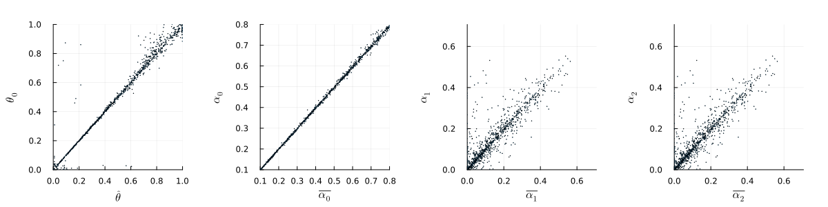
Figure 3: Estimates against true values for $1000$ estimations of $100$ observations using $200$ values of $\hat{\theta}$ while $\varepsilon=0.01$.

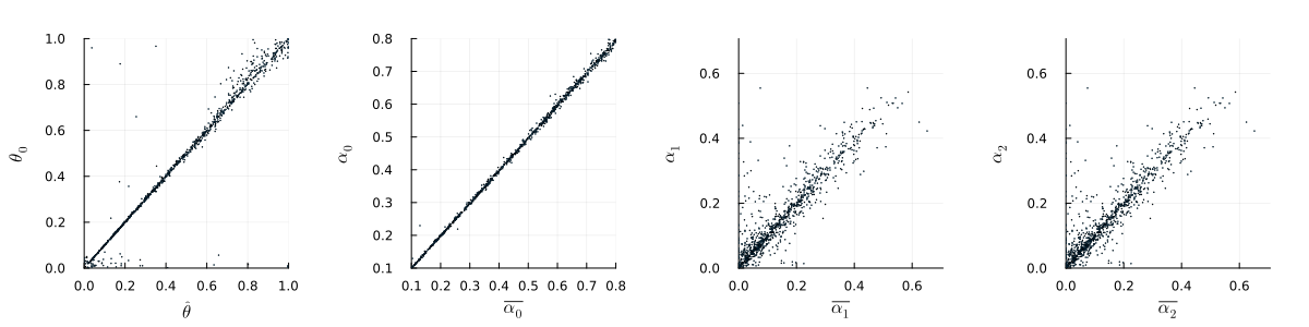
Figure 4: Estimates against true values for $1000$ estimations of $100$ observations using $200$ values of $\hat{\theta}$ while $\varepsilon=0.001$.

3.3 Forecasting

We now take the results from the previous section to complete a prediction simulation study of model (3.1). We make use of a similar methodology and carry out our study as follows.

1. We generate a true parameter vector $(\theta,\alpha_{0},\alpha_{1},\alpha_{2})$ and use this to create synthetic data for training.

2. We train the model using $100$ observations on the time interval $[0,1]$ by using the LS-GD algorithm with $500$ test values of the period $\theta$.

3. Once training is complete, we simulate model (3.1) on the time interval $[0,3]$ with both the true parameter vector and the trained parameter vector.

We generate the initial conditions as

$$(X_{0},Y_{0},Z_{0})\sim\bigg{(}\text{Uniform}(0.4,1),\,\frac{1-X_{0}}{n},\,\frac{(1-X_{0})(n-1)}{n}\bigg{)},$$

where $n\sim\text{Uniform}\{2,3,4,5,6,7\}$. The reason for this is the SIR model has the requirement that

$$X_{t}+Y_{t}+Z_{t}=1,\ \ \ \ t\geq 0.$$

We use a component-wise form of mean-squared error as the metric of the trials. We run $1000$ prediction trials, and for each trial we have $100$ observations/samples. Hence for each trial $j$, $j\in\{1,\ldots,1000\}$, we compute the following sum.

$$T_{j}=\frac{1}{100}\sum\limits_{k=1}^{100}\begin{bmatrix}(X_{t_{k}}-\hat{X}_{t_{k}})^{2},&(Y_{t_{k}}-\hat{Y}_{t_{k}})^{2},&(Z_{t_{k}}-\hat{Z}_{t_{k}})^{2}\end{bmatrix}.$$

Then, we compute $\frac{1}{1000}\sum_{j=1}^{1000}T_{j}$. This metric gives us the ability to check each component error individually while providing insight into the error of the trials of the whole model.

Remark 3.2

There is nothing particularly special about our choice to randomly generate $X_{0}$ then use its value to assign values to $Y_{0}$ and $Z_{0}$. Additionally, nothing special about the assignment of the factors $1/n$ and $(n-1)/n$ – merely a convenience for computation.

The following table includes the true values against the trained (estimated) values for the proportional model.

$(\theta,\alpha_{0},\alpha_{1},\alpha_{2})$	$(0.26836304,0.15114833,0.0621514,0.096762)$
$(\hat{\theta},\hat{\alpha}_{0},\hat{\alpha}_{1},\hat{\alpha}_{2})$, $\varepsilon=0.3$	$(0.27069755,0.1707693,0.11016354,0.082015210)$
$(\hat{\theta},\hat{\alpha}_{0},\hat{\alpha}_{1},\hat{\alpha}_{2})$, $\varepsilon=0.1$	$(0.261749799,0.1717002782,0.025364225,0.1017260206)$
$(\hat{\theta},\hat{\alpha}_{0},\hat{\alpha}_{1},\hat{\alpha}_{2})$, $\varepsilon=0.01$	$(0.2668796604,0.146115022,0.04899088,0.0966312804)$
$(\hat{\theta},\hat{\alpha}_{0},\hat{\alpha}_{1},\hat{\alpha}_{2})$, $\varepsilon=0.001$	$(0.26743667816,0.151314344,0.058359562,0.0989769703)$

Table 2: True paramter values versus trained parameter values for proportional model.

The subsequent figures give simulation results using the true values and the trained values for the parameters. The true parameter observations are marked by a $+$ while the trained parameter observations are marked by a dot.

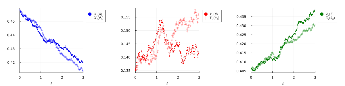
Figure 5: Simulation of model (3.1) for $\varepsilon=0.3$.

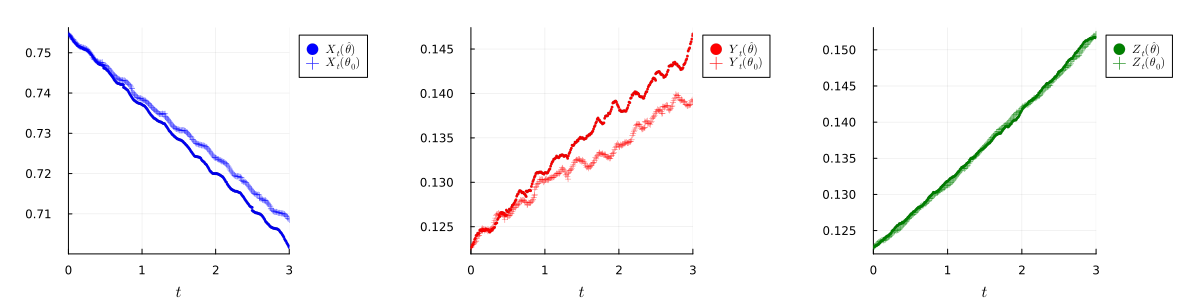
Figure 6: Simulation of model (3.1) for $\varepsilon=0.1$.

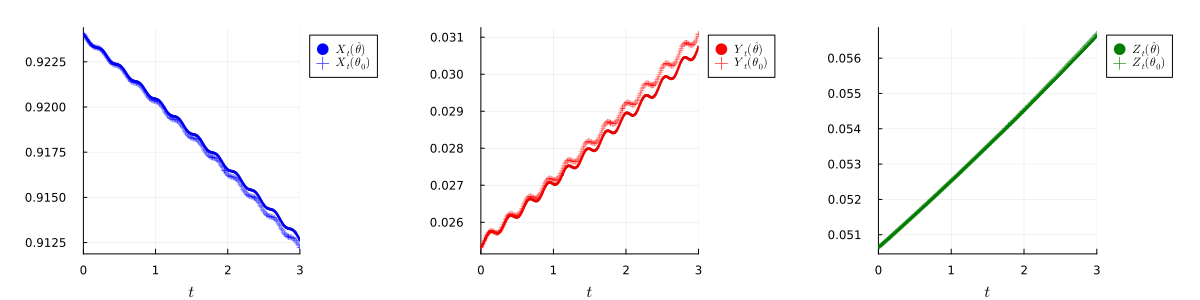
Figure 7: Simulation of model (3.1) for $\varepsilon=0.01$.

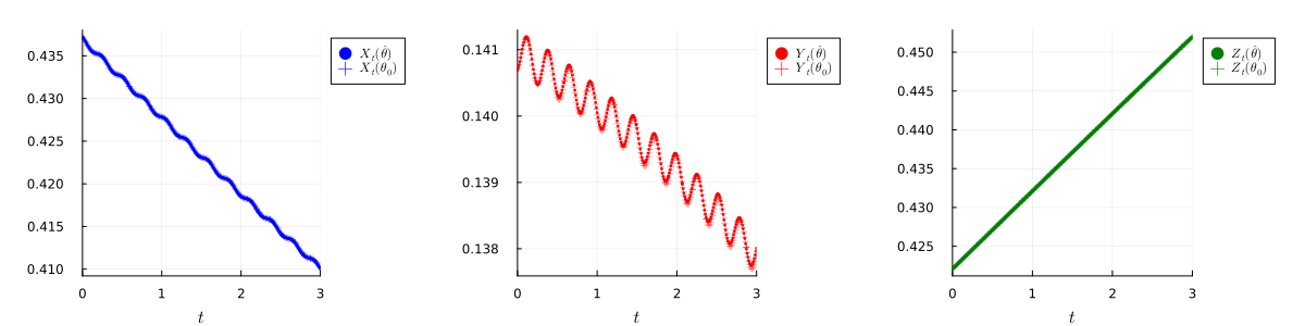
Figure 8: Simulation of model (3.1) for $\varepsilon=0.001$.

$\varepsilon$	Component-wise MSE: $(\hat{X_{t}},\hat{Y_{t}},\hat{Z_{t}})$
$0.3$	$(\begin{matrix}0.000024732&0.00006754&0.00001291\end{matrix})$
$0.1$	$(\begin{matrix}0.000009734&0.00001537&0.000002157\end{matrix})$
$0.01$	$(\begin{matrix}0.000002564&0.000003539&0.0000006851\end{matrix})$
$0.001$	$(\begin{matrix}0.0000001432&0.00000003593&0.00000007774\end{matrix})$

Table 3: True parameter values versus trained parameter values for model (3.1).

4 Simulation study of SIR model for population numbers

4.1 Model for population numbers

In this section, we consider the following model for population numbers:

$$\begin{bmatrix}dX_{t}\\ dY_{t}\\ dZ_{t}\end{bmatrix}=\begin{bmatrix}\Lambda-\mu X_{t}-\beta(t)X_{t}Y_{t}\\ \beta(t)X_{t}Y_{t}-(\mu+\gamma)Y_{t}\\ \gamma Y_{t}-\mu Z_{t}\end{bmatrix}dt\,+\,\varepsilon\!\begin{bmatrix}\sigma X_{t-}Y_{t-}Z_{t-}&0&0\\ 0&\sigma X_{t-}Y_{t-}Z_{t-}&0\\ 0&0&\sigma X_{t-}Y_{t-}Z_{t-}\end{bmatrix}\begin{bmatrix}dL^{(1)}_{t}\\ dL^{(2)}_{t}\\ dL^{(3)}_{t}\end{bmatrix},\\$$ (4.1)

where

$$\begin{bmatrix}L^{(1)}_{t}\\ L^{(2)}_{t}\\ L^{(3)}_{t}\end{bmatrix}=\begin{bmatrix}B^{(1)}_{t}+\displaystyle\int_{0}^{t}\displaystyle\int_{\{|u|>0.1\}}uN^{(1)}(ds,du)\\ B^{(2)}_{t}+\displaystyle\int_{0}^{t}\displaystyle\int_{\{|u|>0.1\}}uN^{(2)}(ds,du)\\ B^{(3)}_{t}+\displaystyle\int_{0}^{t}\displaystyle\int_{\{|u|>0.1\}}uN^{(3)}(ds,du)\end{bmatrix},$$

$$\beta(t)=\alpha_{0}+\alpha_{1}\cos\left(\frac{2\pi t}{\theta}\right)+\alpha_{2}\sin\left(\frac{2\pi t}{\theta}\right),\ \ \ \ \theta\in[0,1],\alpha_{0},\alpha_{1},\alpha_{2}>0,$$

$\Lambda,\mu,\gamma,\sigma>0$ are constants, and $N=N_{1}+N_{2}$ as given in (3.2).

By [9, Theorem 3.1], the SDE (4.1) has a unique strong solution taking values in $\mathbb{R}^{3}_{+}$. We utilize the contrast function (2.1), which is similar to that given in [31] and takes the explicit form:

$$\Psi_{\varepsilon,n}(\theta,\alpha_{0},\alpha_{1},\alpha_{2})=100\varepsilon^{-2}\left(\sum_{k=1}^{100}P_{t_{k}}^{*}(\theta,\alpha_{0},\alpha_{1},\alpha_{2})\Lambda^{-1}_{k-1}P_{t_{k}}(\theta,\alpha_{0},\alpha_{1},\alpha_{2})\right),$$

where

$$P_{t_{k}}(\theta,\alpha_{0},\alpha_{1},\alpha_{2})=\begin{bmatrix}X_{t_{k}}-X_{t_{k-1}}-\frac{1}{100}\left[\Lambda-\mu X_{t_{k-1}}-\beta({t_{k-1}})X_{t_{k-1}}Y_{t_{k-1}}\right]\\ Y_{t_{k}}-Y_{t_{k-1}}-\frac{1}{100}\left[\beta({t_{k-1}})X_{t_{k-1}}Y_{t_{k-1}}-(\mu+\gamma)Y_{t_{k-1}}\right]\\ Z_{t_{k}}-Z_{t_{k-1}}-\frac{1}{100}\left(\gamma Y_{t_{k-1}}-\mu Z_{t_{k-1}}\right)\end{bmatrix},$$

and

$$\Lambda_{k-1}=\begin{bmatrix}[\sigma X_{t_{k-1}}Y_{t_{k-1}}Z_{t_{k-1}}]^{2}&0&0\\ 0&[\sigma X_{t_{k-1}}Y_{t_{k-1}}Z_{t_{k-1}}]^{2}&0\\ 0&0&[\sigma X_{t_{k-1}}Y_{t_{k-1}}Z_{t_{k-1}}]^{2}\end{bmatrix}.$$

4.2 Parameter estimation

We generate the synthetic data $10000$ times and randomly chose $1000$ such data sets to perform estimation upon. Set $\Lambda=0.018,\mu=0.00042$, $\gamma=0.07142$, $\sigma=0.5$ and $(X_{0},Y_{0},Z_{0})=(2.3,0.19,0.25)$ (taken to be in millions). Again, for this study we keep the jumps simple; namely, there is no compensated jump portion. We also make use of the same metric MAE to test our results and the true values for the synthetic data are generated as given in (3.3).

$\varepsilon$	Parameter	MAE
$0.3$
	$\theta$	0.0944492
	$\alpha_{0}$	0.023988
	$\alpha_{1}$	0.0563110
	$\alpha_{2}$	0.058243
$0.1$
	$\theta$	0.03130246
	$\alpha_{0}$	0.00960035
	$\alpha_{1}$	0.0365961
	$\alpha_{2}$	0.0369104
$0.01$
	$\theta$	0.01966768
	$\alpha_{0}$	0.0057932
	$\alpha_{1}$	0.0283396
	$\alpha_{2}$	0.0291711
$0.001$
	$\theta$	0.01657112
	$\alpha_{0}$	0.0056
	$\alpha_{1}$	0.02781
	$\alpha_{2}$	0.0294392

Table 4: Metrics of estimated parameters where $1000$ estimations are completed given $100$ observations and we used $200$ test values of $\hat{\theta}$.

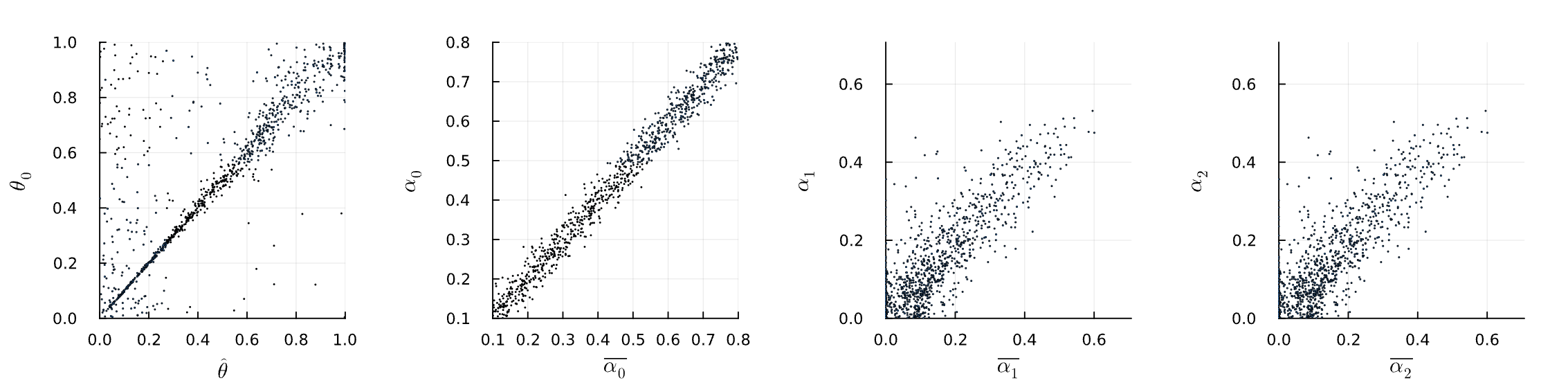
Figure 9: Estimates against true values for $1000$ estimations of $100$ observations using $200$ values of $\hat{\theta}$ while $\varepsilon=0.3$.

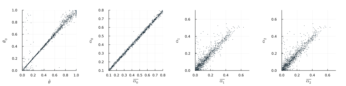
Figure 10: Estimates against true values for $1000$ estimations of $100$ observations using $200$ values of $\hat{\theta}$ while $\varepsilon=0.1$.

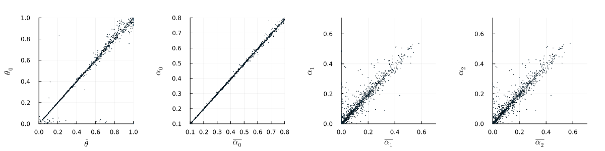
Figure 11: Estimates against true values for $1000$ estimations of $100$ observations using $200$ values of $\hat{\theta}$ while $\varepsilon=0.01$.

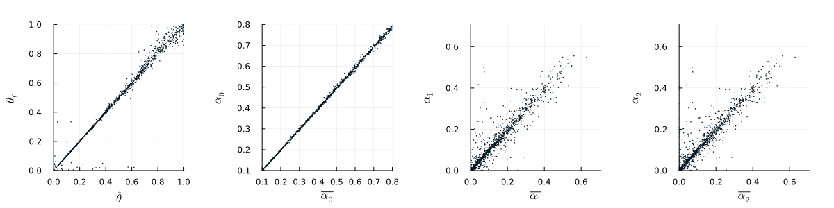
Figure 12: Estimates against true values for $1000$ estimations of $100$ observations using $200$ values of $\hat{\theta}$ while $\varepsilon=0.001$.

4.3 Forecasting

In a similar fashion to the previous section, we perform a predictive simulation study. The primary difference being the initial conditions are randomized such that

$$(X_{0},Y_{0},Z_{0})\sim(\text{Uniform}(1,4),\,\text{Uniform}(0.1,1),\,\text{Uniform}(0.1,1)).$$

Otherwise, the methodology is the same as before including using the component-wise MSE. The following table includes the randomly-generated true parameter values against those we obtained in the estimation. The subsequent figures below display the simulation of model (4.1) using the true parameters and the trained parameters values. The true parameter observations are marked by a $+$ while the trained parameter observations are marked by a dot.

$(\theta,\alpha_{0},\alpha_{1},\alpha_{2})$	$(0.26836304,0.15114833,0.0621514,0.096762)$
$(\hat{\theta},\hat{\alpha}_{0},\hat{\alpha}_{1},\hat{\alpha}_{2})$, $\varepsilon=0.3$	$(0.2759104,0.15106501,0.09268711,0.0418802)$
$(\hat{\theta},\hat{\alpha}_{0},\hat{\alpha}_{1},\hat{\alpha}_{2})$, $\varepsilon=0.1$	$(0.268413479,0.14653753,0.058398519,0.116306536)$
$(\hat{\theta},\hat{\alpha}_{0},\hat{\alpha}_{1},\hat{\alpha}_{2})$, $\varepsilon=0.01$	$(0.26945644,0.1511415,0.0667543397,0.09347593)$
$(\hat{\theta},\hat{\alpha}_{0},\hat{\alpha}_{1},\hat{\alpha}_{2})$, $\varepsilon=0.001$	$(0.26857489,0.151209307,0.06245031,0.0967899)$

Table 5: True parameter values versus trained parameter values for model (4.1).

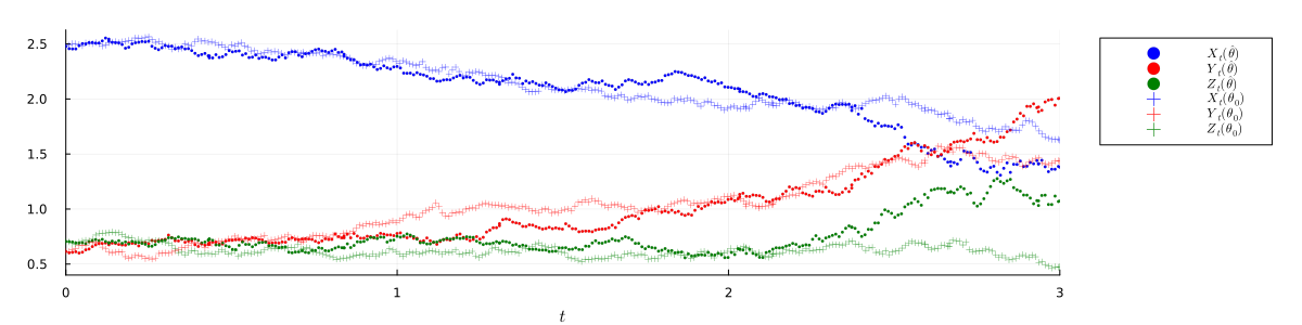
Figure 13: Simulation of model (4.1) for $\varepsilon=0.3$.

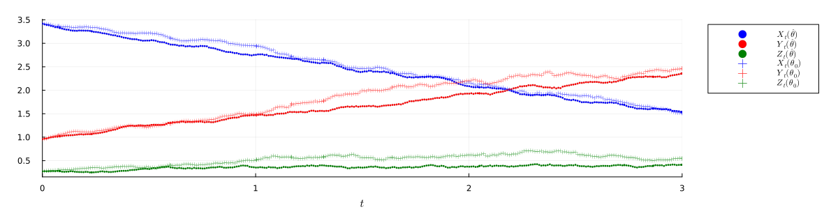
Figure 14: Simulation of model (4.1) for $\varepsilon=0.1$.

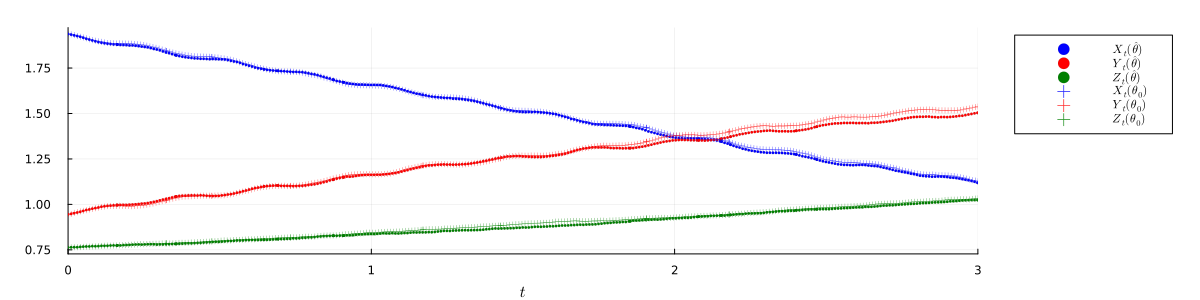
Figure 15: Simulation of model (4.1) for $\varepsilon=0.01$.

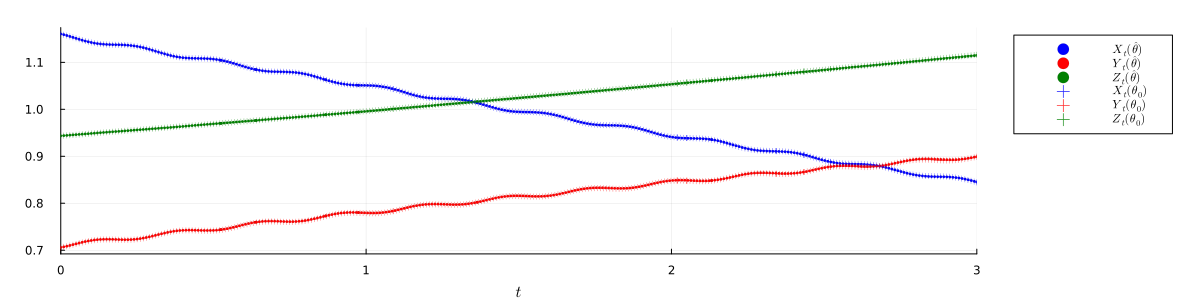
Figure 16: Simulation of model (4.1) for $\varepsilon=0.001$.

$\varepsilon$	Component-wise MSE: $(\hat{X_{t}},\hat{Y_{t}},\hat{Z_{t}})$
$0.3$	$(\begin{matrix}0.119862755&0.4229034&0.1641841226\end{matrix})$
$0.1$	$(\begin{matrix}0.01354954&0.0286335&0.01803421\end{matrix})$
$0.01$	$(\begin{matrix}0.00032701&0.0003369&0.00015043\end{matrix})$
$0.001$	$(\begin{matrix}0.000221016&0.000165453&0.0000109\end{matrix})$

Table 6: True parameter values versus trained parameter values for model (4.1) .

Remark 4.1

Mean-squared error is scale-dependent; hence, comparing the metrics we have for the two model versions is of no valuable use. The former model only takes values in the interval $[0,1]$ whereas the latter model can take values larger than $1$.

5 Conclusion

The novelty of this paper is:

• Estimating the unknown period of a time-dependent periodic transmission function as well as its unknown coefficients.

• The introduction and use of a Linear-Search Gradient-Descent algorithm to iteratively solve for suitable approximations to the LSEs.

• Parameter estimation results for when the noise coefficient (diffusion matrix) is a non-square or non-invertible matrix.

• Extending asymptotic results for consistency and limiting distributions given by Long et al. in [31] to include SDEs driven by general Lévy noises with time-dependent coefficients.

Our aim was to study the ability of estimating parameters governing a periodic transmission for a stochastic SIR model. The model comes in one of two forms, population proportions or population numbers, both of which we have given simulation studies on which we are able to effectively estimate the period of a periodic transmission function.

The theoretical results from Section 2 give reasoning that these estimations efforts hold in general. Moreover, that the asymptotics of the estimators can be ascertained – namely, consistency and limiting distributions. Additionally, these results aid in the generalization of existing efforts in the literature on parameter estimation for SDEs driven by Lévy noises with small coefficient $\varepsilon$.

We introduced the LS-GD algorithm; which was a useful tool in our simulation studies since calculating the LSEs by use of algebraic manipulation may not be a feasible task. Moreover, it provided a way to estimate parameters when there was some multiplicative interaction between them (e.g., recall how $\beta(t)$ was defined).

The work here lays a foundation for further work on parameter estimation of the USSIR model. In future work, we are interested in applying these results to real world data (e.g., COVID-19).

References

- [1] M. Alenezi, F. Al-Anzi and H. Alabdulrazzaq. Building a sensible SIR estimation model for COVID-19 outspread in Kuwait. Alexandria Eng. J. 60, 3161-3175 (2021).
- [2] J. Bao and C. Yuan. Stochastic population dynamics driven by Lévy noise. J. Math. Anal. Appl. 391, 363-375 (2012).
- [3] A. Beck. First-Order Methods in Optimization. Siam (2017).
- [4] A. Bodini, S. Pasquali, A. Pievatolo and F. Ruggeri. Underdetection in a stochastic SIR model for the analysis of the COVID-19 Italian epidemic. Stoch. Environ. Res. Risk Ass. 36, 137-155 (2022).
- [5] G. Chen, T. Li and C. Liu. Lyapunov exponent of a stochastic SIRS model. Comp. Rend. Math. 351, 33-35 (2013).
- [6] X. Chen, J. Li, C. Xiao and P. Yang. Numerical solution and parameter estimation for uncertain SIR model with application to COVID-19. Fuzzy Optim. Decis. Mak. 20, 189-208 (2021).
- [7] S. Clémençon , V.C. Tran and H. de Arazoza. A stochastic SIR model with contact-tracing: large population limits and statistical inference. J. Biol. Dyn. 2, 392-414 (2008).
- [8] S.M. Djouadi, V. Maroulas, X. Pan and J. Xiong. On least-squares estimation for partially observed jump-diffusion processes. ACC (2016).
- [9] T. Easlick and W. Sun. A unified stochastic SIR model driven by Lévy noise with time-dependency. arXiv:2201.03406v2 (2022).
- [10] Z. El Kharrazi and S. Saoud. Simulation of COVID-19 epidemic spread using stochastic differential equations with jump diffusion for SIR model. ICOA (2021).
- [11] A. El Koufi, J. Adnani, A. Bennar and N. Yousfi. Analysis of a stochastic SIR model with vaccination and nonlinear incidence rate. Int. J. Diff. Equ. 9275051 (2019).
- [12] A. El Koufi, J. Adnani, A. Bennar and N. Yousfi. Dynamics of a stochastic SIR epidemic model driven by Lévy jumps with saturated incidence rate and saturated treatment function. Stoch. Anal. Appl. (2021).
- [13] Z. Feng, D. Xu and H. Zhao. Epidemiological models with non-exponentially distributed disease stages and applications to disease control. Bull. Math. Biol. 69, 1511-1536 (2007).
- [14] P. Girardi and C. Gaetan. An SEIR model with time-varying coefficients for analyzing the SARS-CoV-2 epidemic. Risk Anal. (2021).
- [15] A. Gloter and M. Sørensen. Estimation for stochastic differential equations with a small diffusion coefficient. Stoch. Proc. Appl. 119, 679-699 (2009)
- [16] A. Gray, D. Greenhalgh, L. Hu, X. Mao and J. Pan. A stochastic differential equation SIS epidemic model. SIAM J. Appl. Math. 71, 876-902 (2011).
- [17] S. Greenhalgh and T. Day. Time-varying and state-dependent recovery rates in epidemiological models. Infect. Dis. Mod. 2, 419-430 (2017).
- [18] X.X. Guo and W. Sun. Periodic solutions of stochastic differential equations driven by Lévy noises. J. Nonl. Sci. 31:32 (2021).
- [19] W. Hager and H. Zhang. Algorithm 851: CG-DESCENT, a conjugate gradient method with guaranteed descent. ACM Trans. Math. Soft. 32, 113-137 (2006).
- [20] M. Jagan, M. deJonge, O. Krylova and D. Earn. Fast estimation of time-varying infectious disease transmission rates. PLOS Comp/ Biol. (2020).
- [21] C. Ji, D. Jiang and N. Shi. Multigroup SIR epidemic model with stochastic permutation. Physica A. 390, 1747-1762 (2011).
- [22] R.A. Kasonga. The consistency of a non-linear least squares estimator from diffusion processes. Stoch. Proc. Appl. 30, 263-275 (1988)
- [23] W. Kermack and A. McKendrick. Contributions to the mathematical theory of epidemics. Proc. R. Soc. Lond. Ser. A. 115, 700-721 (1927).
- [24] M. Kobayashi and Y. Shimizu. Least squares estimators based on the Adams method for stochastic differential equations with small Lévy noise. arXiv:2201.06787 (2022).
- [25] M. Kröger and R. Schlickeiser. SIR-solution for slowly time-dependent ratio between recovery and infection rates. Physics (MDPI) 4 (2022).
- [26] C. Li, Y. Pei, M. Zhu and Y. Deng. Parameter estimation on a stochastic SIR model with media coverage. Disc. Dyn. Nature Soc. 3187807 (2018).
- [27] X. Liu and P. Stechlinski. Infectious disease models with time-varying parameters and general nonlinear incidence rate. Appl. Math. Model. 1974-1994, (2012).
- [28] Y. Liu, Y. Zhang and Q-Y. Wang. A stochastic SIR epidemic model with Lévy jump and media coverage. Adv. Diff. Equ. 70 (2020).
- [29] N. Privault and L. Wang. Stochastic SIR Lévy jump model with heavy-tailed increments. J. Nonlin Sci. 31:15 (2021).
- [30] H. Long, Y. Shimizu and W. Sun. Least squares estimators for discretely observed stochastic processes driven by small Lévy noises. J. Mul.. Anal. 116, 422-439 (2012).
- [31] H. Long, C. Ma and Y. Shimizu. Least squares estimators for stochastic differential equations driven by small Lévy noises. Stoch. Proc. Appl. 127, 1475-1495 (2016)
- [32] P.K. Mogensen and A.N. Riseth. Optim: A mathematical optimization package for Julia. J. Open Sour. Soft. 3, 615 (2018).
- [33] A. Mummert. Studying the recovery procedure for the time-dependent transmission rate(s) in epidemic models. J. Math. Biol. 67, 483-507 (2013).
- [34] A. Mummert and O. Otunuga. Parameter identification for a stochastic SEIRS epidemic model: case studyiInfluenza. J. Math. Biol. 79, 705-729 (2019).
- [35] J. Pan, A. Gray, D. Greenhalgh and X. Mao. Parameter estimation for the stochastic SIS epidemic model. Stat. Inf. Stoch. Proc. 17, 75-98 (2014).
- [36] S. Paul and E. Lorin. Estimation of COVID-19 recovery and decease periods in Canada using delay model. Sci. Rep. 11, 23763 (2021).
- [37] C. Rackauckas and Q. Nie. DifferentialEquations.jl – a performant and feature-rich ecosystem for solving differential equations in julia. J. Open Res. Soft. 5, 15 (2017).
- [38] Y. Shimizu. Quadratic type contrast functions for discretely observed non-ergodic diffusion processes. Osaka Univ., Math. Sc. Res. Rep. No. 09-04 (2010).
- [39] M. Sørensen and M. Uchida. Small diffusion asymptotics for discretely sampled stochastic differential equations. Bernoulli. 9, 1051-1069 (2003)
- [40] E. Tornatore, S. Buccellato and P. Vetro. Stability of a stochastic SIR system. Physica A. 354, 111-126 (2005).
- [41] M. Uchida. Estimation for discretely observed small diffusions based on approximate martingale estimating functions. Scand. J. Stat. 31, 553-566 (2004)
- [42] A.W. van der Vaart. Asymptotic Statistics. Cambridge University Press (1998).
- [43] B. Wacker and J. Schluter. Time-continuous and time-discrete SIR models revisited: theory and applications. Adv. Differ. Eq. 556 (2020).
- [44] P. Xu and S. Shimada. Least squares parameter estimation in multiplicative noise model. Comm. Stat. Sim. Comp. 29, 83-96 (2007).
- [45] X. Zhang and K. Wang. Stochastic SIR model with jumps. Appl. Math. Lett. 26, 867-874 (2013).
- [46] X. Zhang, Z. Zhang, J. Tong and M. Dong. Ergodicity of stochastic smoking model and parameter estimation. Adv. Diff. Equ. 274 (2016).
- [47] Y. Zhou, S. Yuan and D. Zhao. Threshold behavior of a stochastic SIS model with Lévy jumps. Appl. Math. Comp. 275, 255-267 (2016).
- [48] Y. Zhou and W. Zhang. Threshold of a stochastic SIR epidemic model with Lévy jumps. Physica A. 446, 204-216 (2016).