Hadronic vacuum polarization correction to the bound-electron $g$ factor

Abstract

The hadronic vacuum polarization correction to the $g$ factor of a bound electron is investigated theoretically. An effective hadronic Uehling potential obtained from measured cross sections of $e^{-}e^{+}$ annihilation into hadrons is employed to calculate $g$ factor corrections for low-lying hydrogenic levels. Analytical Dirac-Coulomb wave functions, as well as bound wave functions accounting for the finite nuclear radius are used. Closed formulas for the $g$ factor shift in case of a point-like nucleus are derived. In heavy ions, such effects are found to be much larger than for the free-electron $g$ factor.

I Introduction

Precision Penning-trap experiments on the $g$ factor of hydrogenlike and few-electron highly charged ions allow a thorough testing of quantum electrodynamics (QED), a cornerstone of the standard model describing electromagnetic interactions. The $g$ factor of hydrogen-like silicon ($Z=14$) has been measured with a $5\times 10^{-10}$ relative uncertainty Sturm et al. (2011, 2013), allowing to scrutinize bound-state QED theory (see e.g. Pachucki et al. (2004, 2005); Karshenboim and Milstein (2002); Lee et al. (2005); Yerokhin et al. (2002, 2004); Shabaev and Yerokhin (2002); Beier (2000); Beier et al. (2000); Sailer et al. (2022); Schneider et al. (2022)). Two-loop radiative effects and shifts due to nuclear structure and recoil are observable in such measurements. The high accuracy which can be achieved on the experimental as well as theoretical side also enables the determination of fundamental physical constants such as the electron mass $m_{\rm e}$ Sturm et al. (2014); Köhler et al. (2015); Zatorski et al. (2017); Häffner et al. (2000); Beier et al. (2002). Recently, it was shown that $g$ factor studies can also help in the search for new physics, i.e. the coupling strength of a hypothetical new interaction can be constrained through the comparison of theoretical and experimental results Debierre et al. (2020, 2022); Sailer et al. (2022).

Further improved tests and possible determinations of fundamental constants Yerokhin et al. (2016a); Shabaev et al. (2006); Cakir et al. (2020) call for an increasing accuracy on the theoretical side. The evaluation of two-loop terms up to order $(Z\alpha)^{5}$ (with $Z$ being the atomic number and $\alpha$ the fine-structure constant) has been finalized recently Czarnecki et al. (2018); Pachucki and Puchalski (2017), increasing the theoretical accuracy especially in the low-$Z$ regime. First milestones have been also reached in the calculation of two-loop corrections in stronger Coulomb fields, i.e. for larger values of $Z\alpha$ Yerokhin and Harman (2013); Sikora et al. (2020). As the experiments are advancing towards heavy ions Sturm et al. (2019); Kluge et al. (2008), featuring smaller and smaller characteristic distance scales for the interaction between the bound electron and the nucleons, the effects of other forces may need to be considered as well.

Motivated by these prospects, in this article we investigate vacuum polarization (VP) corrections due to the virtual creation and annihilation of hadrons. The dominant VP contribution arises from virtual $e^{-}e^{+}$ pair creation, which has been widely investigated in the literature Karshenboim and Milstein (2002); Lee et al. (2005); Karshenboim et al. (2001, 2005) and is well understood. The other leptonic VP effect is due to virtual muons, the contribution of which is suppressed by the square of the electron-to-muon mass ratio Berestetskii et al. (1982). The hadronic VP effect, which arises due to a superposition of different virtual hadronic states, is comparable in magnitude to muonic VP, however, it requires a completely different description since the virtual hadrons interact via the strong force. An effective approach to take into account such effects for the free-electron $g$ factor is described in e.g. Ref. Burkhardt et al. (1989), in which hadronic VP is characterized by the cross section of hadron production via $e^{-}e^{+}$ annihilation. Following this treatment, we apply the known empirical parametric hadronic polarization function for the photon propagator from Ref. Burkhardt and Pietrzyk (2001) to account for the complete hadronic contribution in case of the bound-electron $g$ factor.

While in case of the free electron, the hadronic correction only appears on the two-loop level, as a correction to the electrons electromagnetic self-interaction (see Fig. 1a), in case of a bound electron it appears already as a one-loop effect (see Fig. 1b). Furthermore, the hadronic VP is boosted by approximately $\sim Z^{4}$, i.e. by the fourth power of the nuclear charge number, and thus, as we will see later, for heavier ions above $Z=14$ its contribution is larger than in case of a free electron Karshenboim and Shelyuto (2021).

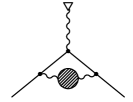
(a)

(b)

Figure 1: Feynman diagrams representing the leading hadronic VP corrections to the free-electron $g$ factor (1a) and the bound-electron $g$ factor (1b). Double lines represent electrons in the electric field of the nucleus and wavy lines with a triangle depict the interaction with the external magnetic field. For the free electron, it is a two-loop process where the self-interaction of the electron is perturbed by the effective hadronic polarization function (shaded bubble). For the bound electron, it is a one-loop correction where the Coulomb interaction with the nucleus (cross) is perturbed by the effective hadronic polarization function.

An effective potential constructed from the parametrized VP function, the hadronic Uehling potential, has been derived in Ref. Breidenbach et al. (2022). We calculate the perturbative correction to the $g$ factor due to this radial potential employing analytical Dirac-Coulomb wave functions, as well as numerically calculated wave functions accounting for a finite-size nucleus. Analytical formulas are presented, and numerical results are given for hydrogenic systems from H to U⁹¹⁺. We note that such an approach assumes an infinitely heavy nucleus, i.e. nuclear recoil effects are excluded in our treatment.

We use natural units with $\hbar=c=1$ for the reduced Planck constant $\hbar$ and the speed of light $c$, and $\alpha={e^{2}}$, where $\alpha$ is the fine-structure constant and $e$ is the elementary charge. Three-vectors are denoted by bold letters.

II $g$ factor corrections

Generally speaking, the $g$ factor describes the coupling of the electron’s magnetic moment $\bm{\mu}$ to its total angular momentum $\bm{J}$. The corresponding first-order Zeeman splitting $\Delta{E}$ due to the electron’s interaction with an external homogeneous magnetic field $\bm{B}$ is

$$\Delta{E}=-\left\langle\bm{\mu}\cdot\bm{B}\right\rangle=g\,\mu_{\mathrm{B}}\left\langle\bm{J}\cdot\bm{B}\right\rangle\,,$$ (1)

where $\mu_{\mathrm{B}}=e/(2m_{\rm e})$ is the Bohr magneton of the electron and $g$ is its $g$ factor, which depends on the electron configuration.

On the other hand, the relativistic interaction of an electron with the external magnetic field can be derived from the minimal coupling principle in the Dirac equation. In first-order perturbation theory, this leads to the energy shift

$$\Delta{E}=e\left\langle\bm{\alpha}\cdot\bm{A}\right\rangle\,,$$ (2)

where $\bm{\alpha}$ are the usual Dirac matrices given in terms of the gamma matrices by $\alpha_{i}=\gamma^{0}\gamma^{i}$ Peskin and Schroeder (1995) and $\bm{A}$ is the vector potential for the magnetic field, such that $\bm{B}=\nabla\times\bm{A}$. Choosing the magnetic field to be directed along the $z$ axis, one can see that a possible choice for the vector potential is $\bm{A}=[\bm{B}\times\bm{r}]/2$, where $\bm{r}$ is the position vector. Together with Eq. (1) and (2), one can derive the following general expression for the $g$ factor Karshenboim et al. (2001):

$$g=\frac{2\kappa m_{\rm e}}{j(j+1)}\int_{0}^{\infty}dr\,rG_{n\kappa}(r)F_{n\kappa}(r)\,,$$ (3)

where $n$ is the principal quantum number of the bound state, $j=|\kappa|-1/2$ is the total angular momentum quantum number and $\kappa$ is the relativistic angular momentum quantum number. The functions $G_{n\kappa}(r),F_{n\kappa}(r)$ are the radial components in the electronic Dirac wave function,

$$\psi_{n\kappa m}(\bm{r})=\frac{1}{r}\left(\begin{array}[]{c}G_{n\kappa}(r)\ \Omega_{\kappa m}(\theta,\varphi)\\ iF_{n\kappa}(r)\ \Omega_{-\kappa m}(\theta,\varphi)\\ \end{array}\right)\,,$$ (4)

where $m$ is the magnetic quantum number and $r=|\bm{r}|$. The spherical spinors $\Omega_{\pm\kappa m}(\theta,\varphi)$ make up the angular components and are the same for any central potential $V(r)$ Johnson et al. (1988).

A straightforward approach for calculating the $g$ factor shift $\Delta{g}^{\mathrm{VP}}$ due to vacuum polarization (VP), is to solve the radial Dirac equation numerically with the inclusion of the VP effect, and then substituting the perturbed functions $G_{n\kappa}^{\mathrm{VP}}(r),F_{n\kappa}^{\mathrm{VP}}(r)$ into Eq. (3). The difference between the pertubed and the unperturbed $g$ factor gives the corresponding shift

$$\Delta{g}^{\mathrm{VP}}=g^{\mathrm{VP}}-g\,.$$ (5)

However, we will apply a different method to investigate the hadronic $g$ factor shift. As shown in Ref. Karshenboim et al. (2005), owing to the properties of Dirac wave functions, the $g$ factor in Eq. (3) can be expressed through the energy eigenvalues $E_{n\kappa}$,

$$g=-\frac{\kappa}{2j(j+1)}\left(1-2\kappa\frac{\partial E_{n\kappa}}{\partial m_{\rm e}}\right)\,,$$ (6)

if the potential $V(r)$ does not depend on the electron mass $m_{\rm e}$. This formula was used successfully, e.g., to investigate the finite nuclear size effect in Ref. Karshenboim et al. (2005). We apply this new approach to investigate the vacuum polarization effect, described by an effective potential. Having a small perturbation $\delta{V}(r)$ to the nucleus potential (like the hadronic Uehling potential Breidenbach et al. (2022)), the $g$ factor shift can be shown to be Karshenboim et al. (2005)

$$\Delta{g}^{\mathrm{VP}}=-\frac{\kappa^{2}}{j(j+1)m_{\rm e}}\left\langle r\frac{\partial\delta V(r)}{\partial r}\right\rangle\,.$$ (7)

For the relativistic ground state and a point-like nucleus, this expectation value can be evaluated further to obtain

$$\Delta{g}_{1s}^{\mathrm{VP}}=\frac{4(1+2\gamma)}{3m_{\rm e}}\Delta{E}_{1s}^{\mathrm{VP}}-\frac{8Z\alpha}{3}\left\langle r\delta V\right\rangle_{1s}\,,$$ (8)

where $\gamma=\sqrt{1-(Z\alpha)^{2}}$ and $\Delta{E}_{1s}=\left\langle\delta V\right\rangle_{1s}$ is the corresponding energy shift in first-order perturbation theory. Since the second term on the right-hand side of Eq. (8) is $Z\alpha$ times smaller than the first term, the $g$ factor shift can be approximated for light ions ($Z\alpha\ll 1$) with the formula:

$$\Delta{g}_{1s}^{\mathrm{VP}}\approx\frac{4(1+2\gamma)}{3m_{\rm e}}\Delta{E}_{1s}^{\mathrm{VP}}\,.$$ (9)

A similar expression also appeared in Ref. Karshenboim et al. (2005); Cakir et al. (2020) in a different context, studying the finite size effect. However, we will investigate the applicability of this formula as an approximation for calculating the $g$ factor shift due to VP effects for light ions.

II.1 Leptonic vacuum polarization correction to the $g$ factor

The leptonic VP correction to the bound-electron $g$ factor is well known. The corresponding diagrams are shown in Fig. 2 and can be divided into two groups: the electric loop (EL) and the magnetic loop (ML) contribution. The vacuum polarization effect in the EL contribution (Fig. 2a and Fig. 2b) is equivalent to a perturbation in the interaction between the bound electron and the nucleus, and thus can be described by an effective perturbing potential $\delta{V}_{\mathrm{EL}}(\bm{r})$. This allows the usage of perturbation theory and the simple inclusion of hadronic VP effects to the bound-electron $g$ factor shift, using Eq. (7). As can be seen in Ref. Lee et al. (2005); Belov et al. (2016), the ML contribution (Fig. 2c) is $Z\alpha$ times smaller than EL in the leading order, and is not the subject of the current work.

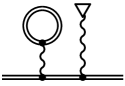
(a)

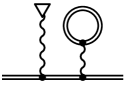
(b)

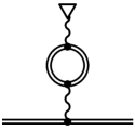
(c)

Figure 2: Feynman diagrams representing the VP correction to the bound-electron $g$ factor. Double lines represent electrons in the electric field of the nucleus and wavy lines with a triangle depict the interaction with the external magnetic field.

The vacuum loop in the EL contribution can be expanded in powers of the nuclear coupling strength $Z\alpha$, which corresponds to a free loop interacting with the nucleus. Due to Furry’s theorem, only odd powers of $Z\alpha$ contribute Furry (1937); Belov et al. (2016). The leading term in this expansion is described by the Uehling potential $\delta{V}_{\mathrm{Ue}}(\bm{r})$ and the contributions of higher order in $Z\alpha$ are summarized to the Wichmann-Kroll potential $\delta{V}_{\mathrm{WK}}(\bm{r})$, such that the effective perturbing potential is given by $\delta{V}_{\mathrm{EL}}(\bm{r})=\delta{V}_{\mathrm{Ue}}(\bm{r})+\delta{V}_{\mathrm{WK}}(\bm{r})$ Belov et al. (2016). The diagrams in Fig. 2a and Fig. 2b contribute equally to the EL correction. In this paper, we will investigate the leading contribution to the vacuum polarization due to the Uehling potential: $\delta{V}_{\mathrm{EL}}(\bm{r})\approx\delta{V}_{\mathrm{Ue}}(\bm{r})$.

In case of leptonic vacuum loops, the well-known leptonic Uehling potential is given by Fullerton and Rinker (1976)

$$\delta{V}_{\mathrm{Ue}}(\bm{r})=-\frac{2\alpha(Z\alpha)}{3\pi}\int d^{3}x\,\rho(\bm{x})\,\frac{K_{1}(2m_{\rm l}|\bm{r}-\bm{x}|)}{|\bm{r}-\bm{x}|}\,,$$ (10)

where $\rho(\bm{x})$ denotes the nuclear charge distribution normalized to unity, $m_{\rm l}$ is the mass of the virtual particle in the fermionic loop and $K_{1}(x)$ is given by

$$K_{1}(x)=\int_{1}^{\infty}dt\ e^{-xt}\left(1+\frac{1}{2t^{2}}\right)\frac{\sqrt{t^{2}-1}}{t^{2}}\,.$$ (11)

The $g$ factor shift of a bound electron in the ground state can be calculated analytically for a point-like nucleus and was already derived in Karshenboim et al. (2001). We will show that one arrives to the same result using the approach in Eq. (7). Using the leptonic Uehling potential for a point-like nucleus ($\rho(\bm{x})=\delta^{(3)}(\bm{x})$) Karshenboim et al. (2001),

$$\delta{V}_{\mathrm{point}}^{\mathrm{lept.}}(r)=-\frac{2\alpha(Z\alpha)}{3\pi r}\ K_{1}(2m_{\rm l}r)\,,$$ (12)

and the radial components of the electronic wave function in the ground state Berestetskii et al. (1982), one obtains from Eq. (7)

$$\Delta{g}^{\mathrm{lept.}}_{\mathrm{point}}(1s)=-\frac{8\alpha(Z\alpha)}{3\pi s}\left[I_{133}-\frac{1}{3}I_{233}+\frac{Z\alpha s}{2\gamma}\left(I_{122}-\frac{1}{3}I_{222}\right)\right]\,.$$ (13)

$I_{abc}$ is a modification of the base integral given in Ref. Karshenboim et al. (2001), see Appendix A, and $s=m_{\rm e}/m_{\rm l}$ is the ratio of the electron and the loop particle masses.

The leading order $Z\alpha$ expansion is given by

$$\Delta{g}^{\mathrm{lept.}}_{\mathrm{point}}(1s)=\ \frac{\alpha}{\pi}\left[-\frac{16s^{2}(Z\alpha)^{4}}{15}+\frac{5\pi s^{3}(Z\alpha)^{5}}{9}\right.$$

$$+\left(\frac{16s^{2}}{15}\ln(2sZ\alpha)-\frac{116s^{2}}{75}-\frac{16s^{4}}{7}\right)(Z\alpha)^{6}$$

$$+\left(-\frac{5\pi s^{3}}{9}\ln\left(\frac{sZ\alpha}{2}\right)-\frac{8\pi s^{3}}{27}+\frac{7\pi s^{5}}{8}\right)(Z\alpha)^{7}$$

$$+\mathcal{O}\left((Z\alpha)^{8}\right)\Big{]}\,.$$ (14)

For $s=1$, this is exactly the same result as in Ref. Karshenboim et al. (2001), however, obtained with a different method. In the case of muonic VP, thus $s=m_{\rm e}/m_{\mu}$, the results for a finite size nucleus were obtained numerically in Ref. Belov et al. (2016).

In the next Subsection, we will use this approach to derive an analytic expression for the hadronic VP correction to the bound-electron $g$ factor.

II.2 Hadronic vacuum polarization correction to the $g$ factor

As discussed in Burkhardt et al. (1989); Burkhardt and Pietrzyk (2001); Breidenbach et al. (2022), the hadronic vacuum polarization function can be constructed semi-empirically from experimental data of $e^{-}e^{+}$ annihilation cross sections. The whole hadronic polarization function is parametrized for seven regions of momentum transfer and is given e.g. in Ref. Burkhardt and Pietrzyk (2001). In Ref. Breidenbach et al. (2022), it was found that only the first region of parametrization is significant for the hadronic energy shift calculations. This is also clear from the physical point of view, since atomic physics is dominated by low energies around eV – keV. Thus, we will use the analytic hadronic Uehling potential introduced in Ref. Breidenbach et al. (2022) for our calculations. For a point-like nucleus it is given by

$$\delta{V}^{\mathrm{had.}}_{\mathrm{point}}(r)=-\frac{2Z\alpha}{r}B_{1}E_{1}\left(\frac{r}{\sqrt{C_{1}}}\right)\,,$$ (15)

with the coefficients $B_{1}=0.0023092$ and $C_{1}=3.9925370$ GeV^-2 Burkhardt and Pietrzyk (2001); Breidenbach et al. (2022) and the exponential integral $E_{1}(x)$ which can be generalized for $n=0,1,2,...$ by Abramowitz and Stegun (1972)

$$E_{n}(x)=\int_{1}^{\infty}dt\ \frac{e^{-xt}}{t^{n}}\,.$$ (16)

The values for $B_{1}$ and $C_{1}$ are taken from the most recent parametrization in Ref. Burkhardt and Pietrzyk (2001) and will be used for the calculations. The error of numerical results is estimated by comparison with an older parametrization in Ref. Burkhardt and Pietrzyk (1995) like has been done in Ref. Breidenbach et al. (2022).

The corresponding hadronic Uehling potential for an extended nucleus with spherical charge distribution $\rho(\bm{x})$ is obtained by the convolution Breidenbach et al. (2022)

$$\delta{V}^{\mathrm{had.}}_{\mathrm{fns}}(\bm{r}) =\int d^{3}x\ \rho(\bm{x})\ \delta V^{\mathrm{had.}}_{\mathrm{point}}(\bm{r}-\bm{x})$$

$$=-\frac{4\pi Z\alpha B_{1}\sqrt{C_{1}}}{r}\int_{0}^{\infty}dx\ x\rho(x)D^{-}_{2}(r,x),$$ (17)

where $x=|\bm{x}|$ and

$$D^{\pm}_{n}(r,x)=E_{n}\left(\frac{|r-x|}{\sqrt{C_{1}}}\right)\pm E_{n}\left(\frac{|r+x|}{\sqrt{C_{1}}}\right)\,.$$ (18)

As in our previous work Breidenbach et al. (2022), we will consider the homogeneously charged sphere as the model for the extended nucleus with root-mean-square (RMS) radii taken from Ref. Angeli and Marinova (2013). The charge distribution $\rho(r)$ is given by

$$\rho(r)=\frac{3}{4\pi R^{3}}\,\theta(R-r)\,,$$ (19)

where $\theta(x)$ is the Heaviside step function and the effective radius $R$ is related to the RMS nuclear charge radius $R_{\mathrm{rms}}$ via $R=\sqrt{5/3}\,R_{\mathrm{rms}}$. The correspondig hadronic Uehling potential is given analytically in Breidenbach et al. (2022), see Appendix B.

Let us turn to the evaluation of the leading hadronic VP contribution to the bound-electron $g$ factor, depicted in Fig. 1b. In the low-energy limit, the hadronic Uehling potential is given by Friar et al. (1999)

$$\delta{V}^{\mathrm{had.}}_{\mathrm{non-rel.}}(\bm{x})=-4\pi Z\alpha B_{1}C_{1}\delta^{(3)}(\bm{x})\,.$$ (20)

Using Eq. (7) and the non-relativistic expectation value of the delta function, the leading order in $Z\alpha$ of the hadronic $g$ factor shift for general $ns$ states is found to be Dizer (2020)

$$\Delta{g}^{\mathrm{had.}}_{\mathrm{non-rel.}}(ns) =-\frac{4}{3m_{\rm e}}\left\langle 12\pi Z\alpha B_{1}C_{1}\delta^{(3)}(\bm{x})\right\rangle_{ns}$$

$$=-\frac{16(Z\alpha)^{4}m_{\rm e}^{2}}{n^{3}}B_{1}C_{1}\,.$$ (21)

For the $1s$ state, a fully relativistic expression for the point-like nucleus can be given. Using the hadronic Uehling potential in Eq. (15) and the relativistic wave function of the ground state, one obtains with Eq. (7):

$$\Delta{g}^{\mathrm{had.}}_{\mathrm{point}}(1s)=\frac{4}{3m_{\rm e}}\Delta{E}^{\mathrm{had.}}_{\mathrm{point}}(1s)-\frac{8B_{1}(Z\alpha)^{2}(2\lambda\sqrt{C_{1}})^{2\gamma}}{3\gamma(1+2\lambda\sqrt{C_{1}})^{2\gamma}}\,,$$ (22)

where $\lambda=Z\alpha m_{\rm e}$ and $\Delta{E}^{\mathrm{had.}}_{\mathrm{point}}(1s)$ is the analytical energy shift for a point-like nucleus given in Ref. Breidenbach et al. (2022),

$$\Delta{E}^{\mathrm{had.}}_{\mathrm{point}}(1s)= -\frac{Z\alpha\lambda(2\lambda\sqrt{C_{1}})^{2\gamma}B_{1}}{\gamma^{2}}$$

$$\times{}_{2}F_{1}\left(2\gamma,2\gamma;1+2\gamma;-2\lambda\sqrt{C_{1}}\right)\,,$$ (23)

with ${}_{2}F_{1}(a,b;c;z)$ being the hypergeometric function Abramowitz and Stegun (1972). The expansion of this expression up to $6^{\rm{th}}$ order in $Z\alpha$ is given by

$$\Delta{g}^{\mathrm{had.}}_{\mathrm{point}}(1s)=\ -16B_{1}C_{1}m_{\rm e}^{2}(Z\alpha)^{4}+\frac{512B_{1}C_{1}^{3/2}m_{\rm e}^{3}(Z\alpha)^{5}}{9}$$

$$-\frac{16B_{1}C_{1}m_{\rm e}^{2}(Z\alpha)^{6}}{3}\Big{[}2+30C_{1}m_{\rm e}^{2}$$

$$\left.\quad-3\ln(2m_{\rm e}Z\alpha\sqrt{C_{1}})\right]+\mathcal{O}\left((Z\alpha)^{7}\right)\,,$$ (24)

and it coincides with the non-relativistic approximation in Eq. (II.2) to order $(Z\alpha)^{4}$.

A similar relativistic calculation for the $2s$ state yields

$$\Delta{g}^{\mathrm{had.}}_{\mathrm{point}}(2s)=\ -2B_{1}C_{1}m_{\rm e}^{2}(Z\alpha)^{4}+\frac{64B_{1}C_{1}^{3/2}m_{\rm e}^{3}(Z\alpha)^{5}}{9}$$

$$-\frac{B_{1}C_{1}m_{\rm e}^{2}(Z\alpha)^{6}}{24}\Big{[}41+420C_{1}m_{\rm e}^{2}$$

$$\left.\quad-48\ln(m_{\rm e}Z\alpha\sqrt{C_{1}})\right]+\mathcal{O}\left((Z\alpha)^{7}\right)\,.$$ (25)

The leading orders of Eq. (II.2) and Eq. (II.2) satisfy the non-relativistic relationship in Eq. (II.2),

$$\Delta{g}^{\mathrm{had.}}_{\mathrm{non-rel.}}(ns)=\frac{1}{n^{3}}\Delta{g}^{\mathrm{had.}}_{\mathrm{non-rel.}}(1s)\,.$$ (26)

II.3 Hadronic vacuum polarization correction to the reduced $g$ factor

Additionally, we investigate hadronic effects on the weighted difference of the $g$ factor and the bound-electron energy $E$ of H-like ions, called reduced $g$ factor,

$$\tilde{g}=g-\frac{4(1+2\gamma)}{3m_{\rm e}}E\,,$$ (27)

put forward in Ref. Cakir et al. (2020) for a possible novel determination of the fine-structure constant, and for testing physics beyond the standard model Debierre et al. (2022). It was shown there that the detrimental nuclear structure contributions featuring large uncertainties can be effectively suppressed in the above combination of the $g$ factor and level energy of the hydrogenic ground state. The question arises whether the same can be said about the hadronic VP corrections investigated in the present article.

The hadronic VP correction to the reduced $g$ factor for a point-like nucleus can be found analytically using Eq. (22) and Eq. (II.2). The leading order $Z\alpha$ expansion is given by

$$\tilde{g}^{\mathrm{had.}}_{\mathrm{point}}(1s)=\ \Delta{g}^{\mathrm{had.}}_{\mathrm{point}}(1s)-\frac{4(1+2\gamma)}{3m_{\rm e}}\Delta{E}^{\mathrm{had.}}_{\mathrm{point}}(1s)$$

$$=\ \frac{128}{9}B_{1}C_{1}^{3/2}m_{\rm e}^{3}(Z\alpha)^{5}-64B_{1}C_{1}^{2}m_{\rm e}^{4}(Z\alpha)^{6}$$

$$+\mathcal{O}\left((Z\alpha)^{7}\right)\,.$$ (28)

Thus, the leading term of order $(Z\alpha)^{4}$ in $\Delta{g}^{\mathrm{had.}}_{\mathrm{point}}(1s)$ cancels such that the hadronic VP contribution to the reduced $g$ factor is indeed small for practical purposes. This also supports the approximation in Eq. (9). Therefore, we may conclude that hadronic effects do not hinder the extraction of $\alpha$ or detailed tests of QED and standard model extensions via the measurement of $\tilde{g}$.

II.4 Hadronic vacuum polarization correction to the weighted $g$ factor difference of H- and Li-like ions

Another quantity of interest is the weighted difference of the $g$ factors of the Li-like and H-like charge states of the same element,

$$\delta_{\Xi}g=g(2s)-\Xi\,g(1s)\,,$$ (29)

where $g(2s)$ is the $g$ factor of the Li-like ion and $g(1s)$ is the $g$ factor of the H-like ion. For light elements, the parameter $\Xi$ can be calculated to great accuracy by Yerokhin et al. (2016a, b)

$$\Xi=2^{-2\gamma-1}\left[1+\frac{3}{16}(Z\alpha)^{2}\right]\left(1-\frac{2851}{1000}\frac{1}{Z}+\frac{107}{100}\frac{1}{Z^{2}}\right)\,.$$ (30)

This weighted (or specific) difference was introduced to suppress uncertainties arising from the nuclear charge radius and further nuclear structural effects Shabaev et al. (2002). Therefore, bound-state QED theory can be investigated more accurately in $g$ factor experiments combining H- and Li-like ions than with the individual ions alone.

As we have seen, the hadronic VP correction to $\delta_{\Xi}g$ for a point-like nucleus can be found analytically. We approximate $\Delta{g}^{\mathrm{had.}}_{\mathrm{point}}(2s)$ of the Li-like ion with the expression in Eq. (II.2) for the H-like ion. Since there are no electron-electron interactions in this approximation, we have to neglect the terms of relative orders $1/Z$ and $1/Z^{2}$ in Eq. (30). We note that the residual weight

$$\Xi_{0}=2^{-2\gamma-1}\left[1+\frac{3}{16}(Z\alpha)^{2}\right]\,,$$ (31)

exactly cancels the first two leading orders $(Z\alpha)^{4}$ and $(Z\alpha)^{5}$:

$$\delta_{\Xi_{0}}g^{\mathrm{had.}}_{\mathrm{point}} =\Delta{g}^{\mathrm{had.}}_{\mathrm{point}}(2s)-\Xi_{0}\,\Delta{g}^{\mathrm{had.}}_{\mathrm{point}}(1s)$$

$$=\frac{5}{2}B_{1}C_{1}^{2}m_{\rm e}^{4}(Z\alpha)^{6}+\mathcal{O}\left((Z\alpha)^{7}\right)\,.$$ (32)

Therefore, we can conclude that hadronic VP effects are also largely cancelled in the above specific difference. A similar conclusion can be drawn for the case of the specific difference introduced for a combination of H- and B-like ions Shabaev et al. (2006). This result is well understood, since nuclear and hadronic VP contributions are both short-range effects with a similar behavior.

III Numerical Results

As mentioned in Ref. Breidenbach et al. (2022), the hadronic VP contribution to the energy shift is about $1/0.665\approx 1.5$ times smaller than the muonic VP contribution in the case of the Uehling term. This can be also confirmed for the $g$ factor shift. Comparing the non-relativistic approximation for the hadronic $g$ factor shift $\Delta{g}^{\mathrm{had.\ VP}}_{\mathrm{non-rel.,point}}$ in Eq. (20) with the first term of the expression for the muonic $g$ factor shift $\Delta{g}^{\mathrm{muonic\ VP}}_{\mathrm{non-rel.,point}}$ in Eq. (II.1), yields for hydrogen in the ground state

$$\Delta{g}^{\mathrm{had.\ VP}}_{\mathrm{non-rel.,point}}(1s) =-1.092(14)\times 10^{-16}$$

$$=0.664(9)\ \Delta{g}^{\mathrm{muonic\ VP}}_{\mathrm{non-rel.,point}}(1s)\,.$$ (33)

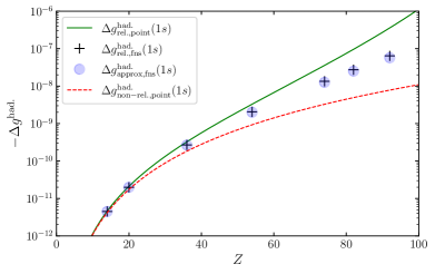
Figure 3: Comparison of analytical and numerical results for the hadronic $g$ factor shift of the bound electron in the ground state of H-like ions with atomic numbers $Z$ obtained in this work, see Table 1. The green solid line represents the analytical expression for a point-like nucleus $\Delta{g}_{\mathrm{rel.,point}}^{\mathrm{had.}}$ in Eq. (II.2), while the red dashed line represents the non-relativistic expression $\Delta{g}_{\mathrm{non-rel.,point}}^{\mathrm{had.}}$ in Eq. (20). The full numerical results for extended nuclei $\Delta{g}_{\mathrm{rel.,fns}}^{\mathrm{had.}}$ (crosses) are compared to the approximation $\Delta{g}_{\mathrm{approx,fns}}^{\mathrm{had.}}$ in Eq. (9) (circles) with hadronic energy shifts for extended nuclei taken from Ref. Breidenbach et al. (2022).

The values for the hadronic $g$ factor shift with an extended nucleus were calculated numerically using two different methods, both yielding the same results within the given uncertainties. The first method consists of calculating the expectation value in Eq. (7) with the FNS hadronic Uehling potential and the semi-analytic wave functions of a homogeneously charged spherical nucleus given in Ref. Patoary and Oreshkina (2018). As a consistency check, these results were reproduced by using the approach of solving the radial Dirac equation numerically with the inclusion of the FNS potential, and substituting the resulting large and small radial wave function components into Eq. (3) and Eq. (5). The results for the hydrogenlike systems H, Si, Ca, Xe, Kr, W, Pb, Cm and U are given in Table 1. A diagrammatic representation is shown in Fig. 3. We note that for $Z=14$ and above, the magnitude of the hadronic vacuum polarization terms considered in this work exceed in magnitude the hadronic contribution to the free-electron $g$ factor Nomura and Teubner (2013). However, it is important to mention that the uncertainty of the leading finite nuclear size correction to the $g$ factor is approximately an order of magnitude larger than the hadronic VP effect for all elements considered (see e.g. Cakir et al. (2020)), hindering the identification of the effect.

The errors given in Table 1 and 2 are based on the uncertainty of the nuclear root-mean-square radii $R_{\mathrm{rms}}$ given in Ref. Angeli and Marinova (2013) and an assumed uncertainty for the parameters $B_{1}$ and $C_{1}$ as described in Section II.2. The total error is dominated by the assumed uncertainty of $B_{1}$ and $C_{1}$. Owing to the closed analytical expression for the hadronic Uehling potential, numerical uncertainties are negligible. For the results $\Delta{g}_{\mathrm{approx,fns}}^{\mathrm{had.}}$ using the approximate formula in Eq. (9), the hadronic energy shifts $\Delta{E}_{\mathrm{rel.,fns}}^{\mathrm{approx}}$ from Ref. Breidenbach et al. (2022) and their respective uncertainties are utilized. For $Z=92$, the hadronic energy shift, which is not given in Ref. Breidenbach et al. (2022), was calculated using the same method.

One can see that the non-relativistic approximation in Eq. (II.2) represents a lower bound for the hadronic $g$ factor shift and is not sufficient for large atomic numbers $Z$. On the other hand, the analytic expression for the relativistic $g$ factor shift in case of a point-like nucleus in Eq. (22) represents an upper bound and differs also significantly from the numerical results for extended nuclei. We conclude that the effects due to a finite size nucleus need to be included in a precision calculation of the hadronic VP effect. At the present time, the uncertainty stemming from the assumed nuclear charge distribution model limits the accuracy to about $1\%$ Breidenbach et al. (2022). At the same time, the absence of more precise parametrizations of the hadronic polarization function in the low-energy regime limits the accuracy also to about $1\%$, see Table 1. Thus, the given errors include, to a great part, all possible limitations of the uncertainty of the hadronic $g$ factor shift.

The simple approximate formula in Eq. (9) is found to be a good approximation for atomic numbers below $Z=14$. The error is less than $1\%$ for atomic numbers up to $Z=36$.

As shown in Section II.3 and II.4, the hadronic VP contribution to the reduced and the weighted $g$ factor in case of a point-like nucleus is at least $Z\alpha$ times smaller than the regular hadronic $g$ factor shift, see Eq. (II.2). In fact, numerical results for extended nuclei confirm that the hadronic contribution to both quantities does not differ significantly from zero for small atomic numbers below $Z=36$ at the current level of accuracy. To see this, note that the numerical results for the finite-size reduced and weighted $g$ factor can be obtained from Table 1 and 2 via

$$\tilde{g}^{\mathrm{had.}}_{\mathrm{fns}}(1s) =\Delta{g}_{\mathrm{rel.,fns}}^{\mathrm{had.}}(1s)-\Delta{g}_{\mathrm{approx,fns}}^{\mathrm{had.}}(1s)\,,$$ (34)

$$\delta_{\Xi_{0}}g^{\mathrm{had.}}_{\mathrm{fns}} =\Delta{g}_{\mathrm{rel.,fns}}^{\mathrm{had.}}(2s)-\Xi_{0}\,\Delta{g}^{\mathrm{had.}}_{\mathrm{rel.,fns}}(1s)\,,$$ (35)

respectively. For $Z=36$, one obtains

$$\tilde{g}^{\mathrm{had.}}_{\mathrm{fns}}(1s) =-32(47)\times 10^{-13}\,,$$ (36)

$$\delta_{\Xi_{0}}g^{\mathrm{had.}}_{\mathrm{fns}} =-1(64)\times 10^{-14}\,.$$ (37)

Even for larger atomic numbers, hadronic effects do not constrain high-precision tests of QED via the measurement of the reduced and weighted $g$ factor.

Recently, a high-precision measurement of the $g$ factor difference of two Ne isotopes was performed Sailer et al. (2022). It was shown that QED effects mostly cancel, whereas nuclear effects like the nuclear recoil are well observable. In the following, we investigate hadronic VP contributions to the bound-electron $g$ factor of the isotopes ²⁰Ne⁹⁺ and ²²Ne⁹⁺ in the ground state.

First, we calculate the hadronic VP correction to the $g$ factor difference stemming from the different nuclear size of the isotopes. Nuclear recoil effects are excluded for now, and nuclear charge radii are taken from Ref. Angeli and Marinova (2013). Using $R_{\text{rms}}=3.0055(21)$ fm for ²⁰Ne⁹⁺ and $R_{\mathrm{rms}}=2.9525(40)$ fm for ²²Ne⁹⁺, the fully relativistic result for both isotopes is

$$\Delta g^{\mathrm{had.}}_{\mathrm{rel.,fns}}\left(1s,{}^{20}\mathrm{Ne}^{9+}\right) =-1.133(14)\times 10^{-12}\,,$$ (38)

$$\Delta g^{\mathrm{had.}}_{\mathrm{rel.,fns}}\left(1s,{}^{22}\mathrm{Ne}^{9+}\right) =-1.133(15)\times 10^{-12}\,.$$ (39)

This is approximately a third of the hadronic contribution of the free electron given in Extended Table 1 in Ref. Sailer et al. (2022). Thus, we conclude that at the given level of accuracy, hadronic effects of the bound electron also do not hinder the precise calculation of the isotopic shift of ²⁰Ne⁹⁺ and ²²Ne⁹⁺.

To estimate also the hadronic VP correction stemming from the different nuclear mass of the isotopes including nuclear recoil effects, we use the non-relativistic formula Karshenboim and Shelyuto (2021)

$$\Delta g^{\mathrm{had.}}_{\mathrm{recoil}}(1s) =\left(\frac{m_{\rm r}}{m_{\rm e}}\right)^{2}\Delta g^{\mathrm{had.}}_{\mathrm{non-rel.}}(1s)\,,$$ (40)

with $m_{\rm r}=m_{\rm N}m_{\rm e}/(m_{\rm N}+m_{\rm e})$ being the reduced mass for an isotope with nuclear mass $m_{\rm N}$. This is a reasonable approximation since the non-relativistic result for Ne ($Z=10$), using Eq. (II.2), is

$$\Delta g^{\mathrm{had.}}_{\mathrm{non-rel.}}(1s,Z=10) =-1.092(14)\times 10^{-12}\,.$$ (41)

Using atomic masses from Ref. Wang et al. (2012), we obtain $m_{\rm r}({}^{20}\mathrm{Ne}^{9+})=0.99997m_{\rm e}$ and $m_{\rm r}({}^{22}\mathrm{Ne}^{9+})=0.99998m_{\rm e}$, such that to first order:

$$\Delta g^{\mathrm{had.}}_{\mathrm{recoil}}(1s,{}^{20}\text{Ne}^{9+}) =-1.092(14)\times 10^{-12}\,,$$ (42)

$$\Delta g^{\mathrm{had.}}_{\mathrm{recoil}}(1s,{}^{22}\text{Ne}^{9+}) =-1.092(14)\times 10^{-12}\,.$$ (43)

Thus, also the nuclear recoil effect to the hadronic VP contribution cannot be resolved at the given level of accuracy.

Table 1: Results for the hadronic VP contribution to the $g$ factor shift of the bound electron in the ground state arising from the Uehling potential in the EL diagram (Fig. 1b) using different approaches: the non-relativistic approximation $\Delta{g}_{\mathrm{non-rel.,point}}^{\mathrm{had.}}$ in Eq. (II.2), the relativistic formula for a point-like nucleus $\Delta{g}_{\mathrm{rel.,point}}^{\mathrm{had.}}$ in Eq. (22), the approximate formula $\Delta{g}_{\mathrm{approx,fns}}^{\mathrm{had.}}$ using the hadronic energy shift with an extended nucleus from Breidenbach et al. (2022) in Eq. (9), and the full relativistic result for an extended nucleus $\Delta{g}_{\mathrm{rel.,fns}}^{\mathrm{had.}}$ using the analytical finite-size Uehling potential with numerical finite-size wave functions in Eq. (7). Root-mean-square nuclear charge radii $R_{\mathrm{rms}}$ are taken from Angeli and Marinova (2013).

$Z$	$R_{\mathrm{rms}}$ [fm]	$\Delta{g}_{\mathrm{non-rel.,point}}^{\mathrm{had.}}(1s)$	$\Delta{g}_{\mathrm{rel.,point}}^{\mathrm{had.}}(1s)$	$\Delta{g}_{\mathrm{approx,fns}}^{\mathrm{had.}}(1s)$	$\Delta{g}_{\mathrm{rel.,fns}}^{\mathrm{had.}}(1s)$
1	0.8783(86)	$-1.092(14)\times 10^{-16}$	$-1.093(14)\times 10^{-16}$	$-1.093(13)\times 10^{-16}$	$-1.093(13)\times 10^{-16}$
14	3.1224(24)	$-4.196(53)\times 10^{-12}$	$-4.616(57)\times 10^{-12}$	$-4.490(56)\times 10^{-12}$	$-4.497(56)\times 10^{-12}$
20	3.4776(19)	$-1.748(22)\times 10^{-11}$	$-2.109(25)\times 10^{-11}$	$-1.989(25)\times 10^{-11}$	$-1.996(25)\times 10^{-11}$
36	4.1884(22)	$-1.835(23)\times 10^{-10}$	$-3.263(39)\times 10^{-10}$	$-2.664(33)\times 10^{-10}$	$-2.696(34)\times 10^{-10}$
54	4.7859(48)	$-9.29(12)\,\,\,\times 10^{-10}$	$-3.291(35)\times 10^{-9}$	$-2.004(25)\times 10^{-9}$	$-2.065(26)\times 10^{-9}$
74	5.3658(23)	$-3.275(41)\times 10^{-9}$	$-3.568(32)\times 10^{-8}$	$-1.261(15)\times 10^{-8}$	$-1.344(17)\times 10^{-8}$
82	5.5012(13)	$-4.938(62)\times 10^{-9}$	$-9.589(77)\times 10^{-8}$	$-2.508(31)\times 10^{-8}$	$-2.728(34)\times 10^{-8}$
92	5.8571(33)	$-7.825(98)\times 10^{-9}$	$-3.572(24)\times 10^{-7}$	$-5.705(71)\times 10^{-8}$	$-6.410(80)\times 10^{-8}$

Table 2: Results for the hadronic VP contribution to the $g$ factor shift of the bound electron in the $2s$ state.

$Z$	$\Delta{g}_{\mathrm{rel.,fns}}^{\mathrm{had.}}(2s)$
1	$-1.366(17)\times 10^{-17}$
14	$-5.673(71)\times 10^{-13}$
20	$-2.542(32)\times 10^{-12}$
36	$-3.583(45)\times 10^{-11}$
54	$-2.966(37)\times 10^{-10}$
74	$-2.189(27)\times 10^{-9}$
82	$-4.728(59)\times 10^{-9}$
92	$-1.213(15)\times 10^{-8}$

IV Summary

Hadronic vacuum polarization corrections to the bound-electron $g$ factor have been calculated, employing a hadronic polarization function constructed from empirical data on electron-positron annihilation into hadrons. We have found that for a broad range of H-like ions, this one-loop effect is considerably larger than hadronic VP for the free electron (see Fig. 1a). Hadronic effects will be observable in future bound-electron $g$ factor experiments once nuclear charge radii and charge distributions will be substantially better known. We have also found that the hadronic effect does not pose a limitation on testing QED or physics beyond the standard model, and determining fundamental constants through specific differences of $g$ factors for different ions, or through the reduced $g$ factor. Finally, the analytic hadronic Uehling potential proves to be very useful and can be applied to further atomic systems, e.g. positronium, or the hyperfine structure.

Appendix A Base integral $I_{abc}$

The base integral $I_{abc}$ used in Eq. (13) is given by Karshenboim et al. (2001)

$$I_{abc}=\ \int_{0}^{1}dy\ \frac{\left(1-y^{2}\right)^{a-1/2}}{y^{b-1}}\left(\frac{sZ\alpha y}{1+sZ\alpha y}\right)^{c-2\epsilon}$$

$$=\ \frac{1}{2}(sZ\alpha)^{c-2\epsilon}B\left(a+\frac{1}{2},1-\frac{b-c}{2}-\epsilon\right)$$

$$\times{}_{3}F_{2}\left(\frac{c}{2}-\epsilon,\frac{c+1}{2}-\epsilon,1-\frac{b-c}{2}-\epsilon;\frac{1}{2},a+\frac{3-b+c}{2}-\epsilon;(sZ\alpha)^{2}\right)$$

$$-\frac{c-2\epsilon}{2}(sZ\alpha)^{c+1-2\epsilon}B\left(a+\frac{1}{2},\frac{3-b+c}{2}-\epsilon\right)$$

$$\times{}_{3}F_{2}\left(\frac{c}{2}+1-\epsilon,\frac{c+1}{2}-\epsilon,\frac{3-b+c}{2}-\epsilon;\frac{3}{2},a+2-\frac{b-c}{2}-\epsilon;(sZ\alpha)^{2}\right)\,,$$ (44)

where $s=m_{\rm e}/m_{\rm l}$ is the ratio of the electron and the loop particle masses, $\epsilon=1-\gamma$ with $\gamma=\sqrt{1-(Z\alpha)^{2}}$, $B(x,y)$ is the beta function and ${}_{3}F_{2}(a_{1},a_{2},a_{3};b_{1},b_{2};z)$ is a generalized hypergeometric function Abramowitz and Stegun (1972).

Appendix B Hadronic Uehling potential for extended nuclei

The analytic hadronic Uehling potential for an extended nucleus with a spherical homogeneous charge distribution with effective radius $R$ is given by Breidenbach et al. (2022)

 $r>R$:

$$\delta V^{\mathrm{had.}}_{\mathrm{fns,out}}(r)=-\frac{3Z\alpha B_{1}\sqrt{C_{1}}}{rR^{3}}\left[\sqrt{C_{1}}R\,D^{+}_{3}(r,R)-C_{1}D^{-}_{4}(r,R)\right].$$ (45)

$r\leq R$:

$$\delta V^{\mathrm{had.}}_{\mathrm{fns,in}}(r)=-\frac{3Z\alpha B_{1}\sqrt{C_{1}}}{rR^{3}} \left[\sqrt{C_{1}}r+\sqrt{C_{1}}RE_{3}\left(\frac{r+R}{\sqrt{C_{1}}}\right)+C_{1}E_{4}\left(\frac{r+R}{\sqrt{C_{1}}}\right)\right.$$

$$-\frac{1}{6}e^{\frac{r-R}{\sqrt{C_{1}}}}\left(2C_{1}+\sqrt{C_{1}}(r+2R)+(r-R)(r+2R)\right)$$

$$-\left.\frac{(r-R)^{2}(r+2R)}{6\sqrt{C_{1}}}E_{1}\left(\frac{R-r}{\sqrt{C_{1}}}\right)\right].$$ (46)

The parameters $B_{1}$ and $C_{1}$ characterize the hadronic polarization function and are given in Section II.2.
The functions $D^{\pm}_{n}(r,R)$ and $E_{n}(x)$ are defined in Eq. (18) and Eq. (16), respectively.

References

- Sturm et al. (2011) S. Sturm, A. Wagner, B. Schabinger, J. Zatorski, Z. Harman, W. Quint, G. Werth, C. H. Keitel, and K. Blaum, Phys. Rev. Lett. 107, 023002 (2011), URL https://link.aps.org/doi/10.1103/PhysRevLett.107.023002.
- Sturm et al. (2013) S. Sturm, A. Wagner, M. Kretzschmar, W. Quint, G. Werth, and K. Blaum, Phys. Rev. A 87, 030501(R) (2013), URL https://link.aps.org/doi/10.1103/PhysRevA.87.030501.
- Pachucki et al. (2004) K. Pachucki, U. D. Jentschura, and V. A. Yerokhin, Phys. Rev. Lett. 93, 150401 (2004), URL https://link.aps.org/doi/10.1103/PhysRevLett.93.150401.
- Pachucki et al. (2005) K. Pachucki, A. Czarnecki, U. D. Jentschura, and V. A. Yerokhin, Phys. Rev. A 72, 022108 (2005), URL https://link.aps.org/doi/10.1103/PhysRevA.72.022108.
- Karshenboim and Milstein (2002) S. G. Karshenboim and A. I. Milstein, Phys. Lett. B 549, 321 (2002), ISSN 0370-2693, URL http://www.sciencedirect.com/science/article/pii/S0370269302029301.
- Lee et al. (2005) R. N. Lee, A. I. Milstein, I. S. Terekhov, and S. G. Karshenboim, Phys. Rev. A 71, 052501 (2005), URL https://link.aps.org/doi/10.1103/PhysRevA.71.052501.
- Yerokhin et al. (2002) V. A. Yerokhin, P. Indelicato, and V. M. Shabaev, Phys. Rev. Lett. 89, 143001 (2002), URL https://link.aps.org/doi/10.1103/PhysRevLett.89.143001.
- Yerokhin et al. (2004) V. A. Yerokhin, P. Indelicato, and V. M. Shabaev, Phys. Rev. A 69, 052503 (2004), URL https://link.aps.org/doi/10.1103/PhysRevA.69.052503.
- Shabaev and Yerokhin (2002) V. M. Shabaev and V. A. Yerokhin, Phys. Rev. Lett. 88, 091801 (2002), URL https://link.aps.org/doi/10.1103/PhysRevLett.88.091801.
- Beier (2000) T. Beier, Phys. Rep. 339, 79 (2000), ISSN 0370-1573, URL http://www.sciencedirect.com/science/article/pii/S0370157300000715.
- Beier et al. (2000) T. Beier, I. Lindgren, H. Persson, S. Salomonson, P. Sunnergren, H. Häffner, and N. Hermanspahn, Phys. Rev. A 62, 032510 (2000), URL https://link.aps.org/doi/10.1103/PhysRevA.62.032510.
- Sailer et al. (2022) T. Sailer, V. Debierre, Z. Harman, F. Heiße, C. König, J. Morgner, B. Tu, A. V. Volotka, C. H. Keitel, K. Blaum, et al., Nature 606, 479–483 (2022), URL https://doi.org/10.1038/s41586-022-04807-w.
- Schneider et al. (2022) A. Schneider, B. Sikora, S. Dickopf, M. Müller, N. S. Oreshkina, A. Rischka, I. A. Valuev, S. Ulmer, J. Walz, Z. Harman, et al., Nature 606, 878–883 (2022), URL https://doi.org/10.1038/s41586-022-04761-7.
- Sturm et al. (2014) S. Sturm, F. Köhler, J. Zatorski, A. Wagner, Z. Harman, G. Werth, W. Quint, C. H. Keitel, and K. Blaum, Nature 506, 467 (2014), URL https://doi.org/10.1038/nature13026.
- Köhler et al. (2015) F. Köhler, S. Sturm, A. Kracke, G. Werth, W. Quint, and K. Blaum, J. Phys. B 48, 144032 (2015), URL https://doi.org/10.1088/0953-4075/48/14/144032.
- Zatorski et al. (2017) J. Zatorski, B. Sikora, S. G. Karshenboim, S. Sturm, F. Köhler-Langes, K. Blaum, C. H. Keitel, and Z. Harman, Phys. Rev. A 96, 012502 (2017), URL https://link.aps.org/doi/10.1103/PhysRevA.96.012502.
- Häffner et al. (2000) H. Häffner, T. Beier, N. Hermanspahn, H.-J. Kluge, W. Quint, S. Stahl, J. Verdú, and G. Werth, Phys. Rev. Lett. 85, 5308 (2000), URL https://link.aps.org/doi/10.1103/PhysRevLett.85.5308.
- Beier et al. (2002) T. Beier, H. Häffner, N. Hermanspahn, S. G. Karshenboim, H.-Jürgen Kluge, W. Quint, S. Stahl, J. Verdú, and G. Werth, Phys. Rev. Lett. 88, 011603 (2001), URL https://link.aps.org/doi/10.1103/PhysRevLett.88.011603.
- Debierre et al. (2020) V. Debierre, C. H. Keitel, and Z. Harman, Phys. Lett. B 807, 135527 (2020), URL https://www.sciencedirect.com/science/article/pii/S0370269320303312.
- Debierre et al. (2022) V. Debierre, C. H. Keitel, and Z. Harman (2022), URL https://doi.org/10.48550/arXiv.2202.01668.
- Yerokhin et al. (2016a) V. A. Yerokhin, E. Berseneva, Z. Harman, I. I. Tupitsyn, and C. H. Keitel, Phys. Rev. Lett. 116, 100801 (2016a), URL https://link.aps.org/doi/10.1103/PhysRevLett.116.100801.
- Shabaev et al. (2006) V. M. Shabaev, D. A. Glazov, N. S. Oreshkina, A. V. Volotka, G. Plunien, H.-J. Kluge, and W. Quint, Phys. Rev. Lett. 96, 253002 (2006), URL https://link.aps.org/doi/10.1103/PhysRevLett.96.253002.
- Cakir et al. (2020) H. Cakir, N. S. Oreshkina, I. A. Valuev, V. Debierre, V. A. Yerokhin, C. H. Keitel, and Z. Harman (2020), URL https://doi.org/10.48550/arXiv.2006.14261.
- Czarnecki et al. (2018) A. Czarnecki, M. Dowling, J. Piclum, and R. Szafron, Phys. Rev. Lett. 120, 043203 (2018), URL https://link.aps.org/doi/10.1103/PhysRevLett.120.043203.
- Pachucki and Puchalski (2017) K. Pachucki and M. Puchalski, Phys. Rev. A 96, 032503 (2017), URL https://link.aps.org/doi/10.1103/PhysRevA.96.032503.
- Yerokhin and Harman (2013) V. A. Yerokhin and Z. Harman, Phys. Rev. A 88, 042502 (2013), URL https://link.aps.org/doi/10.1103/PhysRevA.88.042502.
- Sikora et al. (2020) B. Sikora, V. A. Yerokhin, N. S. Oreshkina, H. Cakir, C. H. Keitel, and Z. Harman, Phys. Rev. Research 2, 012002(R) (2020), URL https://link.aps.org/doi/10.1103/PhysRevResearch.2.012002.
- Sturm et al. (2019) S. Sturm, I. Arapoglou, A. Egl, M. Höcker, S. Kraemer, T. Sailer, B. Tu, A. Weigel, R. Wolf, J. Crespo López-Urrutia, et al., Eur. Phys. J. Spec. Top. 227, 1425 (2019), URL https://doi.org/10.1140/epjst/e2018-800225-2.
- Kluge et al. (2008) H.-J. Kluge, T. Beier, K. Blaum, L. Dahl, S. Eliseev, F. Herfurth, B. Hofmann, O. Kester, S. Koszudowski, C. Kozhuharov, et al., Adv. Quantum Chem. 53, 83 (2008).
- Karshenboim et al. (2001) S. G. Karshenboim, V. G. Ivanov, and V. M. Shabaev, J. Exp. Theor. Phys. 93, 477 (2001), ISSN 1090-6509, URL https://doi.org/10.1134/1.1410592.
- Karshenboim et al. (2005) S. G. Karshenboim, R. N. Lee, and A. I. Milstein, Phys. Rev. A 72, 042101 (2005), URL https://link.aps.org/doi/10.1103/PhysRevA.72.042101.
- Berestetskii et al. (1982) V. B. Berestetskii, L. P. Pitaevskii, and E. M. Lifshitz, Quantum Electrodynamics (Pergamon Press, 1982), 2nd ed.
- Burkhardt et al. (1989) H. Burkhardt, F. Jegerlehner, G. Penso, and C. Verzegnassi, Z. Phys. C 43, 497 (1989), URL https://doi.org/10.1007/BF01506546.
- Burkhardt and Pietrzyk (2001) H. Burkhardt and B. Pietrzyk, Phys. Lett. B 513, 46 (2001), URL https://doi.org/10.1016/S0370-2693(01)00393-8.
- Karshenboim and Shelyuto (2021) S. G. Karshenboim and V. A. Shelyuto, Eur. Phys. J. D 75 (2021), URL https://doi.org/10.1140/epjd/s10053-021-00052-4.
- Breidenbach et al. (2022) S. Breidenbach, E. Dizer, H. Cakir, and Z. Harman, Phys. Rev. A 106, 042805 (2022), URL https://link.aps.org/doi/10.1103/PhysRevA.106.042805.
- Peskin and Schroeder (1995) M. E. Peskin and D. V. Schroeder, An Introduction to Quantum Field Theory (Westview Press, 1995).
- Johnson et al. (1988) W. R. Johnson, S. A. Blundell, and J. Sapirstein, Phys. Rev. A 37, 307 (1988), URL https://link.aps.org/doi/10.1103/PhysRevA.37.307.
- Belov et al. (2016) N. A. Belov, B. Sikora, R. Weis, V. A. Yerokhin, S. Sturm, K. Blaum, C. H. Keitel, and Z. Harman (2016), URL https://doi.org/10.48550/arXiv.1610.01340.
- Furry (1937) W. H. Furry, Phys. Rev. 51, 125 (1937), URL https://link.aps.org/doi/10.1103/PhysRev.51.125.
- Fullerton and Rinker (1976) L. W. Fullerton and G. A. Rinker, Phys. Rev. A 13, 1283 (1976), URL https://link.aps.org/doi/10.1103/PhysRevA.13.1283.
- Abramowitz and Stegun (1972) M. Abramowitz and I. A. Stegun, Handbook of Mathematical Functions (National Bureau of Standards, 1972).
- Burkhardt and Pietrzyk (1995) H. Burkhardt and B. Pietrzyk, Phys. Lett. B 356, 398 (1995), URL https://doi.org/10.1016/0370-2693(95)00820-B.
- Angeli and Marinova (2013) I. Angeli and K. Marinova, At. Data Nucl. Data Tables 99, 69 (2013), ISSN 0092-640X, URL http://www.sciencedirect.com/science/article/pii/S0092640X12000265.
- Friar et al. (1999) J. L. Friar, J. Martorell, and D. W. L. Sprung, Phys. Rev. A 59, 4061 (1999), URL https://link.aps.org/doi/10.1103/PhysRevA.59.4061.
- Dizer (2020) E. Dizer, Analytic Evaluation of Quantum Electrodynamic Corrections in One-Electron Ions (2020), URL http://hdl.handle.net/21.11116/0000-0006-B165-0.
- Yerokhin et al. (2016b) V. A. Yerokhin, E. Berseneva, Z. Harman, I. I. Tupitsyn, and C. H. Keitel, Phys. Rev. A 94, 022502 (2016b), URL https://link.aps.org/doi/10.1103/PhysRevA.94.022502.
- Shabaev et al. (2002) V. M. Shabaev, D. A. Glazov, M. B. Shabaeva, V. A. Yerokhin, G. Plunien, and G. Soff, Phys. Rev. A 65, 062104 (2002), URL https://link.aps.org/doi/10.1103/PhysRevA.65.062104.
- Patoary and Oreshkina (2018) A. S. M. Patoary and N. S. Oreshkina, Eur. Phys. J. D 72, 54 (2018), URL https://doi.org/10.1140/epjd/e2018-80545-9.
- Nomura and Teubner (2013) D. Nomura and T. Teubner, Nuclear Physics B 867, 236 (2013), ISSN 0550-3213, URL http://www.sciencedirect.com/science/article/pii/S0550321312005482.
- Wang et al. (2012) M. Wang, G. Audi, A. H. Wapstra, F. G. Kondev, M. MacCormick, X. Xu, and B. Pfeiffer, Chinese Physics C 36, 1603 (2012), URL https://dx.doi.org/10.1088/1674-1137/36/12/003.