Coloring and Recognizing Mixed Interval Graphs

Abstract

A mixed interval graph is an interval graph that has, for every pair of intersecting intervals, either an arc (directed arbitrarily) or an (undirected) edge. We are particularly interested in scenarios where edges and arcs are defined by the geometry of intervals. In a proper coloring of a mixed interval graph $G$, an interval $u$ receives a lower (different) color than an interval $v$ if $G$ contains arc $(u,v)$ (edge $\{u,v\}$). Coloring of mixed graphs has applications, for example, in scheduling with precedence constraints; see a survey by Sotskov [Mathematics, 2020].

For coloring general mixed interval graphs, we present a $\min\{\omega(G),\lambda(G)+1\}$-approximation algorithm, where $\omega(G)$ is the size of a largest clique and $\lambda(G)$ is the length of a longest directed path in $G$. For the subclass of bidirectional interval graphs (introduced recently for an application in graph drawing), we show that optimal coloring is NP-hard. This was known for general mixed interval graphs.

We introduce a new natural class of mixed interval graphs, which we call containment interval graphs. In such a graph, there is an arc $(u,v)$ if interval $u$ contains interval $v$, and there is an edge $\{u,v\}$ if $u$ and $v$ overlap. We show that these graphs can be recognized in polynomial time, that coloring them with the minimum number of colors is NP-hard, and that there is a 2-approximation algorithm for coloring.

1 Introduction

In a geometric intersection graph, the vertices represent geometric objects, and two vertices are adjacent if and only if the corresponding objects intersect. For example, interval graphs are the intersection graphs of intervals on the real line. These graphs are well understood: interval graphs are chordal and can thus be colored optimally (that is, with the least number of colors) in polynomial time. In other words, given an interval graph $G$, its chromatic number $\chi(G)$ can be computed efficiently.

The notion of coloring can be adapted to directed graphs where an arc $(u,v)$ means that the color of $u$ must be smaller than that of $v$. Clearly, such a coloring can only exist if the given graph is acyclic. Given a directed acyclic graph, its chromatic number can be computed efficiently (via topological sorting).

A generalization of both undirected and directed graphs are mixed graphs that have edges and arcs. A proper coloring of a mixed graph $G$ with vertex set $V(G)$ is a function $f\colon V(G)\to\mathbb{N}$ such that, for any distinct vertices $u$ and $v$ of $G$, the following conditions hold:

1. if there is an edge $\{u,v\}$, then $f(u)\neq f(v)$, and

2. if there is an arc $(u,v)$, then $f(u)<f(v)$.

The objective is to minimize the number of colors.

The concept of mixed graphs was introduced by Sotskov and Tanaev [17] and reintroduced by Hansen, Kuplinsky, and de Werra [8] in the context of proper colorings of mixed graphs. Properly coloring mixed graphs is NP-hard even for bipartite planar graphs [13] but admits efficient algorithms for trees [5] and series-parallel graphs [6].

For a mixed interval graph $G$, the underlying undirected graph of $G$, denoted by $U(G)$, has an edge for every edge or arc of $G$. Note that testing whether a given graph $G$ is a mixed interval graph means testing whether $U(G)$ is an interval graph, which takes linear time [11].

Motivation.

Mixed graphs are graphs where some vertices are connected by (undirected) edges and others by directed arcs. Such structures are useful for modeling relationships that involve both directed and undirected connections and find applications in various areas, including network analysis, transportation planing, job scheduling, and circuit design.

Coloring mixed graphs is relevant in task scheduling problems where tasks have dependencies and resource requirements [19, 3, 16]. In circuit design, coloring mixed graphs allows us to reduce signal crosstalk or interference. Other applications include modeling of metabolic pathways in biology [1], process management in operating systems [2], traffic signal synchronization [14], and timetabling [4]. See the extensive survey by Sotskov [15] for other applications and relevant problems. Coloring of mixed graphs is a challenging problem, as many techniques known for solving graph coloring problems fail in the more general setting.

The study of mixed graph coloring for interval graphs was initiated by Zink et al. [20], motivated by the minimization of the number of additional sub-layers for routing edges in layered orthogonal graph drawing according to the so-called Sugiyama framework [18]. In a follow-up paper, Gutowski et al. [7] resolved some of the problems concerning interval graphs where the subset of arcs and their orientations are given by the geometry of the intersecting intervals. Driven by the graph drawing application, they focused on the directional variant where, for every pair of intersecting intervals, there is an edge when one interval is contained in the other and there is an arc oriented towards the right interval when the intervals overlap.

In this paper we focus on the containment variant where, for any pair of intersecting intervals, there is an arc oriented towards the smaller interval when one interval is contained in the other, and an edge when they overlap. This is the only other natural geometric variant that can be defined for interval graphs, but the containment variant can also be defined for other geometric intersection graphs, or even for graphs defined by systems of intersecting sets.

As there are already some effective techniques for the directional variant, our hope was to use them in the containment variant, or even in more general settings. Quite unexpectedly, the containment variant for interval graphs turned out to be more difficult than the directional variant. We have found our techniques for proving lower bounds for the containment variant of interval graphs to be applicable for the bidirectional variant considered previously [20, 7]. This variant is a generalization of the directional variant mentioned above. Every interval has an orientation; left-going or right-going. There is an arc between two intervals if and only if they overlap and their orientations agree. Arcs between left-going intervals are directed as in the directional variant; the condition for right-going intervals is symmetric. As a result, we get that minimizing the number of additional sub-layers in layered orthogonal graph drawing according to the Sugiyama framework is NP-hard.

Our Contribution.

In this paper we forward the study of coloring mixed graphs where edge directions have a geometric meaning. To this end, we introduce a new natural class of mixed interval graphs, which we call containment interval graphs. In such a graph, there is an arc $(u,v)$ if interval $u$ contains interval $v$, and there is an edge $\{u,v\}$ if $u$ and $v$ overlap. For a set $\mathcal{I}$ of intervals, let $\mathcal{C}[\mathcal{I}]$ be the containment interval graph induced by $\mathcal{I}$. We show that these graphs can be recognized in polynomial time (Section 2), that coloring them optimally is NP-hard (Section 4), and that, for every set $\mathcal{I}$ of intervals, it holds that $\chi(\mathcal{C}[\mathcal{I}])\leq 2\omega(\mathcal{C}[\mathcal{I}])-1$, that is, $\mathcal{C}[\mathcal{I}]$ can be colored with fewer than twice as many colors as the size of the largest clique in $\mathcal{C}[\mathcal{I}]$ (Section 3). In other words, containment interval graphs are $\chi$-bounded. Our constructive proof yields a 2-approximation algorithm for coloring containment interval graphs.

Then we prove that, for the class of bidirectional interval graphs, optimal coloring is NP-hard (Section 5). This answers (negatively) an open problem that was asked previously [7]. Our reduction is similar to the one for containment interval graphs, but technically somewhat more challenging. Finally, we show that, for any mixed interval graph $G$ without directed cycles, it holds that $\chi(G)\leq\omega(G)\cdot(\lambda(G)+1)$, where $\lambda(G)$ denotes the length of a longest directed path in $G$ (Section 6). Since $\chi(G)\geq\max\{\omega(G),\lambda(G)+1\}$, our constructive proof for the upper bound yields a $\min\{\omega(G),\lambda(G)+1\}$-approximation algorithm. The upper bound is asymptotically tight in the worst case.

Table 1: Known and new results concerning subclasses of mixed interval graphs. The time complexities refer to a given set of $n$ intervals with $m$ pairwise intersections. (We use T, P, and C as shorthand for Theorem, Proposition, Corollary, respectively.)

Mixed interval	Coloring								Recognition
graph class	complexity		lower bound		upper bound		approximation
containment	NP-hard	T4.1	$2\omega{-}1$	P3.5	$2\omega{-}1$	T3.1	2	C3.3	$O(nm)$	T2.1
directional	$O(n\log n)$	[7]					1	[7]	$O(n^{2})$	[7]
bidirectional	NP-hard	T5.1					2	[7]	open
general	NP-hard	[7]	$(\lambda{+}2)\omega/2$	P6.3	$(\lambda{+}1)\omega$	T6.1	$\min\{\omega,\lambda{+}1\}$	T6.1	$O(n{+}m)$	[11]

Table 1 gives an overview over known and new results concerning the above-mentioned subclasses of mixed interval graphs. Given a positive integer $k$, we use $[k]$ as shorthand for the set $\{1,2,\dots,k\}$. When we visualize a graph coloring corresponding to a set of intervals, we use horizontal tracks to indicate the color. In Figure 1, we briefly analyze the relationships between the three classes of geometrically defined mixed interval graphs; directional ($\mathcal{D}$), bidirectional ($\mathcal{B}$), and containment interval graphs ($\mathcal{C}$).

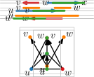
(a) $G_{1}\in\mathcal{C}\setminus\mathcal{B}$

(b) $G_{2}\in\mathcal{D}\setminus\mathcal{C}$

(c) $G_{3}\in\mathcal{B}\setminus\mathcal{D}$

Figure 1: Let $\mathcal{D}$, $\mathcal{B}$, and $\mathcal{C}$ be the classes of directional, bidirectional, and containment interval graphs. Clearly, $\mathcal{D}\subseteq\mathcal{B}$. The above sets of intervals and the corresponding directed graphs show that the classes $\mathcal{D}$ and $\mathcal{B}$ are incomparable with the class $\mathcal{C}$ and that $\mathcal{D}$ is properly contained in $\mathcal{B}$.

2 Recognition of Containment Interval Graphs

Booth and Lueker [11] introduced a data structure called PQ-tree to recognize, for a given undirected graph $G$, whether $G$ is an interval graph. A PQ-tree is a rooted tree of so-called P-nodes, where the order of children can be arbitrarily permuted, and Q-nodes, where the order of children is fixed up to inversion. A specific permutation of all nodes is called a rotation. One can think of the leaves of a PQ-tree to represent the maximal cliques of $G$ and a specific rotation to represent an order of the maximal cliques, which implies an interval representation of $G$ where every vertex is contained in a consecutive sequence of maximal cliques. (Actually, a PQ-tree can encode all possible interval representations of $G$.)

Observe that a representation of a containment interval graph is an interval representation. Hence, if, for a given mixed graph $G$, a containment representation $\mathcal{I}$ exists, then $\mathcal{I}$ corresponds to a rotation of the PQ-tree constructed for the underlying undirected graph $U(G)$ by the algorithm of Booth and Lueker [11]. Hence, to recognize a containment interval graph $G$, we proceed in three phases. First, we compute a PQ-tree $T$ of $U(G)$. Second, we find a rotation of $T$ corresponding to a containment representation of $G$. Third, we determine suitable endpoints for the intervals corresponding to our selected rotation resulting in a containment representation $\mathcal{I}$ of $G$.

In the second phase, we proceed top-down to fix the permutation of each node of $T$ while we maintain as invariant that before and after deciding the permutation of a single node, we can still reach a rotation of $T$ corresponding to a containment representation $\mathcal{I}$ (provided $G$ is a containment interval graph). Depending on the set of maximal cliques (corresponding to leaves) a vertex $v$ is contained in, we can determine where $v$ is introduced in $T$ (roughly at the root of the subtree containing all leaves corresponding to $v$). Intuitively, it is “natural” for a vertex $u$ introduced further up in the tree to have an arc towards a vertex $v$ introduced further down in the tree. However, if $u$ and $v$ are connected by an edge, we need to permute the nodes of the PQ-tree such that both $u$ and $v$ start or end in the same maximal clique. These restrictions can propagate.

If we end up with a rotation of $T$, we construct, in the third phase, a corresponding containment representation if possible. To this end, we determine for every vertex the first and the last clique it appears in, which groups the left and right endpoint of the intervals. Within each group, we sort the endpoints according to the constraints implied by the arcs and edges where possible. What remains are induced mixed subgraphs of vertices that start and end in the same cliques and that behave the same with respect to every other vertex (i.e., they are all connected to this vertex by an outgoing arc or an incoming arc or an edge). We can interpret each such subgraph as a partially ordered set for which we need to check whether it is two-dimensional and find two corresponding linear orders, which gives us an ordering of their left and their right endpoints. This last part depends on the linear-time algorithm by McConnell and Spinrad [12] that can construct such two orders for any two-dimensional poset.

Theorem 2.1 (thm:recognition*).

$\star$] There is an algorithm that, given a mixed graph $G$, decides whether $G$ is a containment interval graph. The algorithm runs in $O(nm)$ time, where $n$ is the number of vertices of $G$ and $m$ is the total number of edges and arcs of $G$, and produces a containment representation of $G$ if $G$ admits one.

The full proof follows the ideas presented above, but has some technical subtleties; see the appendix.

3 A 2-Approximation Algorithm for Coloring Containment Interval Graphs

In this section, we present a 2-approximation algorithm for coloring containment interval graphs, we detail how to make the algorithm run in $O(n\log n)$ time for a set of $n$ intervals, and we construct a family of sets of intervals that shows that our analysis is tight.

Theorem 3.1.

For any set $\mathcal{I}$ of intervals, the containment interval graph $\mathcal{C}[\mathcal{I}]$ induced by $\mathcal{I}$ admits a proper coloring with at most $2\cdot\omega(\mathcal{C}[\mathcal{I}])-1$ colors.

Proof 3.2.

For simplicity, let $G:=\mathcal{C}[\mathcal{I}]$ and $\omega:=\omega(G)$. We use induction on $\omega$. If $\omega=1$, then $G$ has no edges and clearly admits a proper coloring using only one color. So assume that $\omega>1$ and that the theorem holds for all graphs with smaller clique number.

Recall that a proper interval graph is an interval graph that has a representation where no interval is contained in another interval. Let $M(\mathcal{I})$ denote the subset of $\mathcal{I}$ consisting of intervals that are maximal with respect to the containment relation. In particular, $\mathcal{C}[M(\mathcal{I})]$ is a proper interval graph. Observe that $\bigcup M(\mathcal{I})=\bigcup\mathcal{I}$ (where we consider the union of intervals as a subset of the real line). Let $R$ be an inclusion-wise minimal subset of $M(\mathcal{I})$ such that $\bigcup R=\bigcup\mathcal{I}$. In Figure 2, the intervals in $M(\mathcal{I})$ are marked with crosses and the set of intervals on the lowest two (gray) lines is one way of choosing $R$.

Claim 1.

$\mathcal{C}[R]$ is an undirected linear forest.

All intervals in $M(\mathcal{I})$ and thus in $R$ are incomparable with respect to the containment relation, so $\mathcal{C}[R]$ has no arcs. Note that $\mathcal{C}[R]$ is a proper interval graph, so it contains no induced $K_{1,3}$ and no induced cycle with at least four vertices. Thus it suffices to prove that $\mathcal{C}[R]$ is triangle-free. For contradiction, suppose otherwise. Let $x,y,z$ induce a triangle in $\mathcal{C}[R]$, ordered according to their left endpoints. As $x,y,z$ are pairwise overlapping, note that $y\subseteq x\cup z$, and thus $\bigcup(R\setminus\{y\})=\bigcup R$. This contradicts the minimality of $R$.

By the claim above, $\mathcal{C}[R]$ can be properly colored with colors $\{1,2\}$. Let $f_{1}$ be such a coloring. If $R=\mathcal{I}$, we are done (using only $\omega$ many colors), so suppose that $\mathcal{I}\setminus R\neq\emptyset$. Slightly abusing notation, we define $G^{\prime}:=G-R$.

Claim 2.

The largest clique in $G^{\prime}$ has at most $\omega-1$ vertices.

As $G^{\prime}$ is a subgraph of $G$, each clique in $G^{\prime}$ has at most $\omega$ vertices. For contradiction, suppose that there is a set $S\subseteq\mathcal{I}\setminus R$ such that $|S|=\omega$ and all intervals in $S$ pairwise intersect. By the Helly property of intervals, $\bigcap S\neq\emptyset$. Let $p\in\bigcap S$. Since $\bigcup R=\bigcup\mathcal{I}$, there is an interval $r\in R$ that contains $p$. Thus $S\cup\{r\}$ is a clique in $G$ with $\omega+1$ vertices, which contradicts the definition of $\omega$.

By the inductive assumption, $G^{\prime}$ admits a proper coloring $f_{2}$ using colors $[2(\omega-1)-1]$. Finally, we define $f\colon\mathcal{I}\to[2\omega-1]$ as follows:

$$f(x)=\begin{cases}f_{1}(x)&\text{ if }x\in R,\\ f_{2}(x)+2&\text{ if }x\notin R.\end{cases}$$

We claim that $f$ is a proper coloring of $G$. (For an example, see Figure 2.)

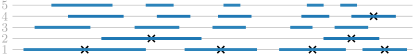
Figure 2: A set of intervals and a coloring produced by the 2-approximation algorithm. The intervals that lie in $M(\mathcal{I})$ at the top level of the recursion are marked with crosses.

First, note that if $x,y\in\mathcal{I}$ are distinct and $x\cap y\neq\emptyset$, then $f(x)\neq f(y)$. Indeed, if $x,y\in R$, then $f(x)=f_{1}(x)\neq f_{1}(y)=f(y)$. If $x,y\notin R$, then $f(x)=f_{2}(x)+2\neq f_{2}(y)+2=f(y)$. Finally, if, say, $x\in R$ and $y\notin R$, then $f(x)\in\{1,2\}$ and $f(y)\geq 3$.

It remains to argue that the second condition in the definition of a proper coloring holds as well. For a contradiction, let $x$ and $y$ be distinct intervals and assume that $x\subseteq y$ and $f(y)>f(x)$. Note that $x\notin M(\mathcal{I})$ and thus $x\notin R$. This implies that $f(x)\geq 3$. Since we assumed that $f(y)>f(x)$, we have that $f(y)>3$. Hence, $y\not\in R$. However, by the inductive assumption, we have that $f(x)=f_{2}(x)+2>f_{2}(y)+2=f(y)$, which yields the desired contradiction. This completes the proof.

Observe that the proof of Theorem 3.1 can be easily transformed into an efficient algorithm, which yields the following corollary.

Corollary 3.3.

There is a 2-approximation algorithm for coloring interval containment graphs properly. Given a set of $n$ intervals, the algorithm runs in $O(n\log n)$ time.

Proof 3.4.

For any graph $G$, we have $\chi(G)\geq\omega(G)$. Hence, the approximation factor follows directly from Theorem 3.1.

It remains to implement the constructive proof of Theorem 3.1 efficiently. Let $\mathcal{I}$ be the given set of intervals. For each interval $I$ in $\mathcal{I}$, let $r_{I}$ be the right endpoint of $I$. We go through the intervals from left to right in several phases. In each phase, we use two colors, except possibly in the last phase where we may use only one color. For phase $i$ with $i\geq 1$, we reserve the set $\mathit{colors}(i)=\{2i-1,2i\}$. We use an augmented balanced binary search tree $\mathcal{T}$ to store the intervals in $\mathcal{I}$. We will query $\mathcal{T}$ in two ways. A query of type Q1 in $\mathcal{T}$ with a value $x\in\mathbb{R}\cup\{-\infty\}$ will return, among all intervals whose left endpoint is at least $x$, one with leftmost left endpoint (and $\mathit{nil}$ if such an interval does not exist). A query of type Q2 in $\mathcal{T}$ with a value $y\in\mathbb{R}$ will return, among all intervals whose left endpoint is at most $y$, one with rightmost right endpoint (and $\mathit{nil}$ if such an interval does not exist). Note that the two queries are not symmetric.

Algorithm 1 describes our algorithm in pseudocode. Initially, $\mathcal{T}$ stores all intervals in $\mathcal{I}$. The algorithm terminates once $\mathcal{T}$ is empty and all intervals are colored.

$\mathcal{T}.\mathsf{initialize}(\mathcal{I})$

$i=0$

while not $\mathcal{T}.\mathsf{empty}()$ do

       $i=i+1$

        // start new phase

       $I=\mathcal{T}.\mathsf{Q1}(-\infty)$

       $c=I.\mathit{color}=2i-1$

        // color $I$ and set current color

      $\mathcal{T}.\mathsf{remove}(I)$

       while not $\mathcal{T}.\mathsf{empty}()$ do

             $I^{\prime}=\mathcal{T}.\mathsf{Q2}(r_{I})$

             if $I^{\prime}==\mathit{nil}$ or $r_{I^{\prime}}\leq r_{I}$ then // no interval contains $r_{I}$

                   $I^{\prime}=\mathcal{T}.\mathsf{Q1}(r_{I})$

                   if $I^{\prime}==\mathit{nil}$ then break // finish current phase

                   $I^{\prime}.\mathit{color}=c$

                    // color $I^{\prime}$ and keep current color

                  

            else  // $I$ and $I^{\prime}$ overlap

                   $c=I^{\prime}.\mathit{color}=\mathit{colors}(i)\setminus\{c\}$

                    // color $I^{\prime}$ and swap current color

                  

            $\mathcal{T}.\mathsf{remove}(I^{\prime})$

             $I=I^{\prime}$

      

Algorithm 1 2-Approximate-Coloring(set $\mathcal{I}$ of $n$ intervals)

We start each phase by Q1-querying $\mathcal{T}$ with $-\infty$. This yields the leftmost interval $I$ stored in $\mathcal{T}$. We color $I$ with the smaller color $2i-1$ reserved for the current phase $i$. Let the current color $c$ be this color. We remove $I$ from $\mathcal{T}$. Then we Q2-query $\mathcal{T}$ with the right endpoint $r_{I}$ of $I$ and consider the following two possibilities.

Case I:

If the Q2-query returns $\mathit{nil}$ or an interval that lies completely to the left of $r_{I}$, we Q1-query $\mathcal{T}$ with $r_{I}$ for an interval to the right of $r_{I}$. If such an interval $I^{\prime}$ exists, it must be disjoint from $I$, so we color $I^{\prime}$ with the current color $c$. Otherwise, we start a new phase.

Case II:

If the Q2-query returns an interval $I^{\prime}$ that overlaps with the previous interval $I$, we color $I^{\prime}$ with the other color $c^{\prime}$ that we reserved for the current phase, that is, $\{c^{\prime}\}=\mathit{colors}(i)\setminus\{c\}$. Then we set the current color $c$ to $c^{\prime}$.

In either case, if we do not start a new phase, we remove $I^{\prime}$ from $\mathcal{T}$ and proceed with the next Q2-query as above, with $I^{\prime}$ now playing the role of $I$.

It remains to implement the balanced binary search tree $\mathcal{T}$. The key of an interval is its left endpoint. For simplicity, we assume that the intervals are stored in the leaves of $\mathcal{T}$ and that the key of each inner node is the maximum of the keys in its left subtree. This suffices to answer queries of type Q1. For queries of type Q2, we augment $\mathcal{T}$ by storing, with each node $\nu$, a value $\max(\nu)$ that we set to the maximum of the right endpoints among all intervals in the subtree rooted at $\nu$. (We also store a pointer $\mu(\nu)$ to the interval that yields the maximum.) In a Q2-query with a value $y$, we search for the largest key $k\leq y$. Let $\pi$ be the search path in $\mathcal{T}$, and initialize $m$ with $-\infty$. When traversing $\pi$, we inspect each node $\nu$ that hangs off $\pi$ on the left side. If $\max(\nu)>m$, then we set $m=\max(\nu)$ and $\rho=\mu(\nu)$. When we reach a leaf, $\rho$ points to an interval whose right endpoint is maximum among all intervals whose left endpoint is at most $y$.

The runtime of $O(n\log n)$ is obvious since we insert, query, and delete each interval in $O(\log n)$ time exactly once.

Proposition 3.5.

There is an infinite family $(\mathcal{I}_{n})_{n\geq 1}$ of sets of intervals with $|\mathcal{I}_{n}|=3\cdot 2^{n-1}-2$, $\chi(\mathcal{C}[\mathcal{I}_{n}])=2n-1$, and $\omega(\mathcal{C}[\mathcal{I}_{n}])=n$.

Proof 3.6.

The construction is iterative. The family $\mathcal{I}_{1}$ consists of a single interval of unit length.

Now let $n>1$ and suppose that we have defined $\mathcal{I}_{n-1}$ and want to define $\mathcal{I}_{n}$. We introduce two new intervals $\ell_{n}$ and $r_{n}$, both of length $3^{n-1}$, that overlap slightly. Then we introduce two copies of $\mathcal{I}_{n-1}$. All intervals of one copy are contained in $\ell_{n}\setminus r_{n}$, and all intervals of the other copy are contained in $r_{n}\setminus\ell_{n}$.

The number of intervals in $\mathcal{I}_{n}$ is given by the recursion: $f(1)=1$ and $f(n)=2f(n-1)+2$, which solves to $f(n)=3\cdot 2^{n-1}-2$. Furthermore, it is straightforward to observe that with each step of the construction, the size of a largest clique increases by $1$.

We claim that, for $i\in[n]$, in any proper coloring of $\mathcal{C}[\mathcal{I}_{i}]$, the difference between the largest and the smallest color used is at least $2i-2$. Clearly, the claim holds for $i=1$. Now assume that it holds for $i=n-1$. Consider any proper coloring of $\mathcal{C}[\mathcal{I}_{n}]$, and let $m$ be the minimum color used in this coloring. The colors of $\ell_{n}$ and $r_{n}$ must be different. Without loss of generality, suppose that the color of $r_{n}$ is larger than the color of $\ell_{n}$. In particular, the color of $r_{n}$ is at least $m+1$. Now consider the copy of $\mathcal{I}_{n-1}$ contained in $r_{n}$. The color of each interval in this copy must be larger than the color of $r_{n}$, so in particular the minimum color used for this copy of $\mathcal{I}_{n-1}$ is at least $m+2$. By the inductive assumption, some interval in this copy of $\mathcal{I}_{n-1}$ receives a color that is at least $m+2+2(n-1)-2=2n-2+m$. Summing up, the difference between the largest and the smallest color used for $\mathcal{C}[\mathcal{I}_{n}]$ is at least $2n-2$.

Given that the minimum color is $1$, we conclude that $\chi(\mathcal{C}[\mathcal{I}_{n}])\geq 2n-1$.

For the upper bound, we color $\mathcal{C}[\mathcal{I}_{n}]$ as follows. For $n=1$, we color the only interval with color $1$. For $n>1$, we color $\ell_{n}$ with color $1$ and $r_{n}$ with color $2$. Next, for each of the two copies of $\mathcal{I}_{n-1}$, we use the proper coloring defined inductively with all colors increased by $2$, see Figure 3.

Figure 3: Instance for the proof of Proposition 3.5 for $n=3$: $|\mathcal{I}_{n}|=3\cdot 2^{n-1}-2=10$, $\omega(\mathcal{I}_{n})=n=3$, and $\chi(\mathcal{I}_{n})=2n-1=5$.

4 Coloring Containment Interval Graphs Is NP-Hard

In this section we show that it is NP-hard to color a containment interval graph with a given number of colors.

Theorem 4.1.

Given a set $\mathcal{I}$ of intervals and a positive integer $k$, it is NP-hard to decide whether $k$ colors suffice to color $\mathcal{C}[\mathcal{I}]$, that is, whether $\chi(\mathcal{C}[\mathcal{I}])\leq k$.

Proof 4.2.

We describe a reduction from (exact) 3-Sat, i.e., the satisfiability problem where every clause contains exactly three literals. Let $\varphi=C_{1}\wedge C_{2}\wedge\dots\wedge C_{m}$ be an instance of 3-Sat where, for each clause $C_{i}$ ($i\in[m]$), the literals are negated or unnegated variables from the set $\{x_{1},x_{2},\dots,x_{n}\}$, and let $H=5(m+1)$ be a threshold.

Using $\varphi$, we construct in polynomial time a set of intervals (with pairwise distinct endpoints) such that the corresponding containment interval graph has a proper coloring with $H$ colors if and only if $\varphi$ is satisfiable. To this end, we introduce variable gadgets and clause gadgets, which are sets of intervals representing the variables and clauses of $\varphi$, respectively. Our main building structure used in these gadgets is a Christmas tree, that is, an ordered set of intervals where each interval contains its successor; see, for example, the set of red intervals in Figure 4. Clearly, the intervals of a Christmas tree form a totally ordered clique and any proper coloring needs to observe this order. In Figure 5, Christmas trees are represented by trapezoids. The height of a Christmas tree is the number of intervals it consists of.

Let $j\in[n]$. The variable gadget for $x_{j}$ consists of two Christmas trees (formed by the red and gray intervals in Figure 4) whose longest intervals overlap and, for each tree, of two additional intervals (green in Figure 4). These green intervals lie immediately to the left and to the right of the shortest interval in their tree. The right green interval of the red tree overlaps the left green interval of the gray tree. Figure 4 depicts two representations of the same gadget for a variable $x$, each with its own coloring of the intervals (encoded by the height of the intervals; see the numbers at the right side of the gray box). The left representation with its coloring corresponds to assigning true to $x$, the right representation corresponds to assigning false.

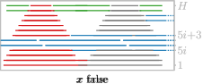
Figure 4: Variable gadget for the proof of Theorem 4.1 in its two states. The blue intervals with dots extend to the clause gadgets. The topmost blue interval (starting immediately to the right of a gray interval) indicates that $x$ is part of a clause $C_{j}$ with $j>i$; the blue interval (with a small gap) that starts immediately to the right of a red interval indicates that $\neg x$ is part of the clause $C_{i}$.

The height of the red tree is $H-1$ minus the number of occurrences of literals $x_{j^{\prime}}$ and $\neg x_{j^{\prime}}$ with $j^{\prime}<j$ in $\varphi$. The height of the gray tree is that of the red tree minus the number of occurrences of $\neg x_{j}$ in $\varphi$. We say that $x_{j}$ is set to true if the bottom interval of the gray tree has color 1; otherwise we say that $x_{j}$ is set to false.

For $i\in[m]$, the gadget for clause $C_{i}$ consists of a Christmas tree (light blue in Figure 5) of height $H-(5i+2)=5(m-i)+3$. All clause gadgets are placed to the right of all variable gadgets, in the order $C_{1},\dots,C_{m}$ from left to right.

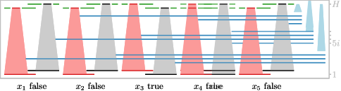
Figure 5: Variable gadgets (red and gray) and clause gadgets (blue) for the 3-Sat instance $(\neg x_{2}\vee\neg x_{4}\vee x_{5})\wedge(x_{1}\vee\neg x_{3}\vee x_{4})\wedge(\neg x_{1}\vee x_{2}\vee x_{3})$ with a fulfilling truth assignment (above) and a non-fulfilling assignment (below). Note that the latter uses one color more (is one level higher).

The key idea to transport a Boolean value from a variable gadget to a clause gadget is to add, for each occurrence of a literal $\ell_{j}\in\{x_{j},\neg x_{j}\}$ in a clause $C_{i}$, an “arm” (blue intervals in Figures 4 and 5) that ends to the right of the clause gadget (the light blue Christmas tree) corresponding to $C_{i}$ and starts immediately to the right of the $5i$-th interval of the gray tree (if $\ell_{j}=x_{j}$) or of the red tree (if $\ell_{j}=\neg x_{j}$) corresponding to $\ell_{j}$. The arm is represented by a sequence of intervals that are separated by a small gap within each Christmas tree of each clause gadget passed by the arm (such that, for any two arms, their gaps are disjoint and the resulting intervals do not contain each other). Assuming that the total number of colors is $H$, two intervals of the same arm that are separated by a gap need to get the same color because, at the gap, $H-2$ colors are occupied by other intervals and the one remaining “wrong” color is blocked due to the green intervals of the variable gadgets; see Figures 4 and 5. The green intervals are contained by the blue intervals of the arms and need to get color $H$ or $H-1$.

If there is a satisfying truth assignment for $\varphi$, then there is a proper coloring that colors the variable gadgets such that they represent this truth assignment. As for every clause $C_{i}$, at least one of its literals in $C_{i}$ is true, the corresponding arm can use color $5i$. Then, the arms of the other literals that occur in $C_{i}$ can use colors $5i+1$ and $5i+2$. This allows the light blue Christmas tree representing clause $C_{i}$, which has height $H-5i-2$ and is contained in the rightmost interval of each of these arms, to use the colors $\{5i+3,5i+4,\dots,H\}$.

Now suppose for a contradiction that there is no satisfying truth assignment for $\varphi$, but that there is a proper coloring with $H$ colors. This coloring assigns a truth value to each variable gadget (depending on whether the bottommost interval of the red or the gray tree has color 1). Clearly, there is a clause $C_{i}$ in $\varphi$ that is not satisfied by this truth assignment. Hence, none of the arms connecting the clause gadget of $C_{i}$ with its three corresponding variable gadgets can use color $5i$. Hence they must use colors $5i+1$, $5i+2$, and $5i+3$ (or higher). This forces the (blue) Christmas tree representing clause $C_{i}$ to use colors $\{5i+4,\dots,H,H+1\}$.

Thus, a proper coloring with $H$ colors exists if and only if $\varphi$ is satisfiable.

5 Coloring Bidirectional Interval Graphs Is NP-Hard

In this section we show that it is NP-hard to color a bidirectional interval graph with a given number of colors. For a set $\mathcal{I}$ of intervals and a function $o$ that maps every interval in $\mathcal{I}$ to an orientation (left-going or right-going), let $\mathcal{B}[\mathcal{I},o]$ be the bidirectional interval graph induced by $\mathcal{I}$ and $o$.

Theorem 5.1.

Given a set $\mathcal{I}$ of intervals with orientations $o$ and a positive integer $k$, it is NP-hard to decide whether $k$ colors suffice to color $\mathcal{B}[\mathcal{I},o]$, that is, whether $\chi(\mathcal{B}[\mathcal{I},o])\leq k$.

Proof 5.2.

We use the same ideas as in the proof of Theorem 4.1, but now we reduce from Monotone 3-Sat, the version of 3-Sat where every clause contains only negated or only unnegated variables as literals. For an overview, see Figures 6 and 7. Let $\varphi=C_{1}\wedge C_{2}\wedge\dots\wedge C_{m}$ be the given instance of Monotone 3-Sat with variables $\{x_{1},x_{2},\dots,x_{n}\}$. As before, let $H=5(m+1)$ be the number of colors sufficient for coloring a yes-instance.

We now construct variable and clause gadgets by specifying a set $\mathcal{I}$ of intervals with orientations $o$. Our intervals have pairwise distinct endpoints. Our main building structures are left- and right-going staircases. A left-going staircase (gray in Figures 6 and 7) is an ordered set of left-going intervals that share a common point and whose left and right endpoints are in the order of the set. A right-going staircase is symmetric (red in Figures 6 and 7). Observe that staircases in (bi)directional interval graphs behave like Christmas trees in containment graphs: they form totally ordered cliques. The height of a staircase is the number of its intervals. In Figure 7, we draw staircases as parallelograms and we indicate left- and right-going intervals by arrow heads.

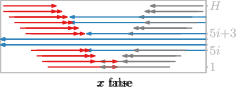
Figure 6: Variable gadget for the proof of Theorem 5.1 in its two states. Intervals directions are indicated by arrow heads. The blue intervals extend (to the right) to the clause gadgets of only negated variables. The two blue arrow heads starting next to the red intervals indicate that the clause $C_{i}$ and a clause $C_{j}$ with $j>i$ contain the literal $\neg x$.

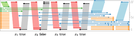
Figure 7: Variable gadgets (red and gray) and clause gadgets (light green and light blue) for the Monotone 3-Sat instance $(x_{1}\vee x_{2}\vee x_{4})\wedge(\neg x_{1}\vee\neg x_{2}\vee\neg x_{3})\wedge(\neg x_{2}\vee\neg x_{3}\vee\neg x_{4})$ with a fulfilling truth assignment (top) and a non-fulfilling assignment (bottom), which use $H$ and $H+1$ colors, respectively. Interval directions are indicated by arrow heads.

Let $i\in[m]$. If the clause $C_{i}$ has only negated literals, we again have three “arms” in $C_{i}$ starting to the right of the $5i$-th interval of the red staircase of the three corresponding variables; see the blue intervals in Figures 6 and 7. The intervals of these arms are left-going and they are not split by a gap at the other variable gadgets this time because now we need to contain the left-going intervals of the staircases to have edges instead of arcs in $\mathcal{B}[\mathcal{I},o]$. The arms end below a left-going light blue staircase (see Figure 7 on the upper right side) of height $5(m-i)+3$ whose maximum color is $H$ if and only if none of the corresponding arms gets a color greater than $5i+2$.

Note that we need to avoid arcs between the arms. Therefore, we let every arm have a gap below each blue staircase that it passes. These gaps do not overlap and their order is inverse to the order of the left endpoints of the involved intervals. We continue the arm with a right-going interval (to avoid an arc with the blue staircase and the other arms) ending to the right of the blue staircase, where we continue again with a left-going interval. Consider such an arm with intervals $I$ and $I^{\prime}$ (going in different directions) around a gap. At this gap, it is important that no color smaller than the color of $I$ is available for $I^{\prime}$, forcing $I^{\prime}$ to also get the color of $I$. Hence, we add long left-going intervals blocking every color not occupied by an arm or the blue staircase; see the orange intervals in Figure 7.

For every clause with only unnegated literals, we use the same construction but mirrored (connecting to the gray staircases); see the green intervals and light green staircases depicted in the top left corner of Figure 7.

We now have the same conditions as in the proof of Theorem 4.1: If there is a satisfying truth assignment for $\varphi$, there is a proper coloring, which colors the variable gadgets such that they represent this truth assignment. Again, for every $i\in[m]$, clause $C_{i}$ contains at least one literal set to true. Hence, the corresponding arm can get color $5i$, and the other two arms and the (light blue or light green) staircase of $C_{i}$ get colors $\{5i+1,5i+2,\dots,H\}$.

If there is no satisfying truth assignment for $\varphi$, then there is a clause $C_{i}$ none of whose arms (as a whole) can get color $5i$. If each arm occupies only one layer, then an interval of the clause gadget of $C_{i}$ requires color $H+1$. If there is an arm occupying more than one layer, then below a clause gadget of some clause $C_{i^{\prime}}$, there are two colors blocked by this arm (at one of its gaps). Then, however, an interval of the clique of size $H-1$ at this gap belonging to the (light blue or light green) staircase of $C_{i^{\prime}}$, to the other arms, or to the orange “blocker” intervals requires color $H+1$; see Figure 7 for such an example.

6 Coloring General Mixed Interval Graphs

In this section we consider a further generalization of mixed interval graphs. We are dealing with an interval graph $G$ whose edges can be arbitrarily oriented (or stay undirected). In other words, the edge directions are not related to the geometry of the intervals.

Observe that a proper coloring of $G$ exists if and only if $G$ does not contain a directed cycle. Let $\chi(G)$ denote the minimum number of colors in a proper coloring of $G$, if it exists, or $\infty$ otherwise. We point out that the existence of a directed cycle can be determined in polynomial time (using, for example, depth-first search).

Note that clearly we have $\omega(G)\leq\chi(G)$. However, there is another parameter that enforces a large chromatic number even in sparse graphs. A directed path (of length $t$) in $G$ is a sequence of vertices $\langle v_{1},v_{2},\dots,v_{t+1}\rangle$, such that, for each $i\in[t]$, the arc $(v_{i},v_{i+1})$ exists. Let $\lambda(G)$ denote the length of a longest directed path in $G$.

Note that the vertices in a directed path receive pairwise distinct colors in any proper coloring. Thus we have $\chi(G)\geq\lambda(G)+1$, and consequently $\chi(G)\geq\max\{\omega(G),\lambda(G)+1\}$.

Theorem 6.1.

Let $G$ be a mixed interval graph without directed cycles. Then $\chi(G)\leq(\lambda(G)+1)\cdot\omega(G)$.

Proof 6.2.

Let $V$ denote the vertex set of $G$. Let $G^{\to}$ be the graph obtained from $G$ by removing all edges. Clearly, $G^{\to}$ is a DAG. We partition $V$ into layers $L_{0},L_{1},\ldots$ as follows. The set $L_{0}$ consists of the vertices that are sources in $G^{\to}$, i.e., they do not have incoming arcs. Then, for $i=1,2,\ldots$, we iteratively define $L_{i}$ to be the set of sources in $G^{\to}\setminus\bigcup_{j=0}^{i-1}L_{j}$. Note that $\lambda(G)=\max\{i\colon L_{i}\neq\emptyset\}$. For $x\in V$, let $\ell(x)\in\{0,\dots,\lambda(G)\}$ denote the unique $i$ such that $x\in L_{i}$.

Recall that the underlying undirected graph of $G$, $U(G)$, is an (undirected) interval graph, and thus $\chi(U(G))=\omega(U(G))=\omega(G)$. Let $c\colon V\to[\omega(U(G))]$ be an optimal proper coloring of $U(G)$.

Now we define a coloring $f$ of $G$: for $x\in V$, let $f(x)=\ell(x)\cdot\omega(G)+c(x)$. Note that $1\leq f(x)\leq(\lambda(G)+1)\cdot\omega(G)$. We claim that $f$ is a proper coloring.

Consider an edge $\{x,y\}$. As this is also an edge in $U(G)$, we obtain that $c(x)\neq c(y)$, and so $f(x)\neq f(y)$. Now consider an arc $(x,y)$. Its existence implies that $\ell(x)<\ell(y)$, and thus $f(x)<f(y)$.

For some instances, the above bound is asymptotically tight.

Proposition 6.3.

There is an infinite family $(G_{k})_{k\geq 1}$ of mixed interval graphs with $|V(G_{k})|=2k^{2}$, $\lambda(G_{k})=k-1$, $\omega(G_{k})=2k$, and $\chi(G_{k})=(k+1)\cdot k=(\lambda(G_{k})+2)\cdot\omega(G_{k})/2$.

Proof 6.4.

Let $\mathcal{I}_{k}=\mathcal{I}_{k,1}\cup\mathcal{I}_{k,2}\cup\dots\cup\mathcal{I}_{k,k}$ be a set of $k^{2}$ intervals defined as follows; see Figure 8 for $\mathcal{I}_{4}$. For $i\in[k]$, let $\mathcal{I}_{k,i}$ be a multiset that contains $k$ copies of the interval $[6i,6i+8]$. Similarly, let $\mathcal{I}_{k}^{\prime}=\mathcal{I}_{k,1}^{\prime}\cup\mathcal{I}_{k,2}^{\prime}\cup\dots\cup\mathcal{I}_{k,k}^{\prime}$ be a set of $k^{2}$ intervals such that $\mathcal{I}_{k}^{\prime}$ is the image of mirroring $\mathcal{I}_{k}$ at the point $x=6k+7$. Note that, for $i\in[k-1]$, every interval in $\mathcal{I}_{k,i}$ intersects every interval in $\mathcal{I}_{k,i+1}$ and every interval in $\mathcal{I}_{k,i}^{\prime}$ intersects every interval in $\mathcal{I}_{k,i+1}^{\prime}$. Additionally, every interval in $\mathcal{I}_{k,k}$ intersects every interval in $\mathcal{I}_{k,k}^{\prime}$.

Let $G_{k}$ be a mixed interval graph for the set $\mathcal{I}_{k}\cup\mathcal{I}_{k}^{\prime}$. We direct the edges of $G_{k}$ as follows. Let $\{I,I^{\prime}\}$ be a pair of intervals in $\mathcal{I}_{k}\cup\mathcal{I}_{k}^{\prime}$ that intersect each other. If $I$ and $I^{\prime}$ are copies of the same interval, then $\{I,I^{\prime}\}$ is an edge of $G_{k}$. Otherwise, $(I,I^{\prime})$ is an arc of $G_{k}$ if $\{I,I^{\prime}\}\subseteq\mathcal{I}_{k}$ and $I$ lies further to the left than $I^{\prime}$, if $\{I,I^{\prime}\}\subseteq\mathcal{I}_{k}^{\prime}$ and $I$ lies further to the right than $I^{\prime}$, or if $(I,I^{\prime})\in\mathcal{I}_{k,k}\times\mathcal{I}_{k,k}^{\prime}$. It is easy to see that $G_{k}$ has the desired properties.

Note that the mixed interval graphs that we constructed in the proof above are even directional interval graphs.

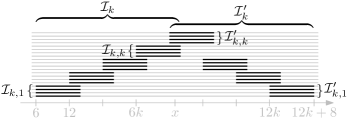
Figure 8: For any $k\geq 1$, the set $\mathcal{I}_{k}\cup\mathcal{I}_{k}^{\prime}$ of intervals gives rise to a mixed interval graph $G_{k}$ with $2k^{2}$ vertices, $\lambda(G_{k})=k-1$, $\omega(G_{k})=2k$, and $\chi(G_{k})=(k+1)\cdot k=(\lambda(G_{k})+2)\cdot\omega(G_{k})/2$.

7 Open Problems

The obvious open problems are improvements to the results in Table 1, in particular: Is there a constant-factor approximation algorithm for coloring general mixed interval graphs? For applications in graph drawing, a better-than-2 approximation for coloring bidirectional interval graphs is of particular interest.

Is there a linear-time recognition algorithm for directional or containment interval graphs? Is there a polynomial-time recognition algorithm for bidirectional interval graphs?

Using a reduction from Max-3-SAT instead of 3-SAT, it may be possible to adjust our NP-hardness proofs in order to show APX-hardness. To this end, the difference in the number of colors needed to color a yes-instance and the number of colors needed to color a no-instance would have to be proportional to the number of clauses that cannot be satisfied. We were not able to force such a large difference, hence we leave the APX-hardness of (or the existence of a PTAS for) coloring containment and birectional interval graphs open.

Acknowledgments.

We are indebted to Krzysztof Fleszar, Zbigniew Lonc, Karolina Okrasa, and Marta Piecyk for fruitful discussions. Additionally, we acknowledge the welcoming and productive atmosphere at the workshop Homonolo 2022, where some of the work was done.

Appendix

Appendix A Recognition of Containment Interval Graphs

Here we present a recognition algorithm for containment interval graphs. Given a mixed graph $G$, our algorithm decides whether $G$ is a containment interval graph. If it is, the algorithm additionally constructs a set $\mathcal{I}$ of intervals representing $G$, i.e., with $\mathcal{C}[\mathcal{I}]$ isomorphic with $G$. The algorithm works in three phases. In the first phase, a PQ-tree representing the interval representations of the underlying undirected graph $U(G)$ of $G$ is constructed. In the second phase, the algorithm carefully selects a rotation of the PQ-tree. This corresponds to fixing the order in which the maximal cliques appear in the interval representation of $U(G)$. This almost fixes the interval representation. In the third phase, the endpoints of the intervals are perturbed so that the edges and arcs of $G$ are represented correctly. We achieve this by reducing our problem to that of finding a two-dimensional realizer of a partial order.

The main result of this section is the following theorem. See 2.1

In Section A.1, we introduce the necessary machinery of PQ-trees. Details of the second and the third phase are described in Sections A.2 and A.3, respectively.

A.1 MPQ-Trees

For a set of pairwise intersecting intervals on the real line, let the clique point be the leftmost point on the real line that lies in all the intervals. Given an interval representation of an interval graph $G$, we get a linear order of the maximal cliques of $G$ by their clique points from left to right. Booth and Lueker [11] showed that a graph $G$ is an interval graph if and only if the maximal cliques of $G$ admit a consecutive arrangement, i.e., a linear order such that, for each vertex $v$, all the maximal cliques containing $v$ occur consecutively in the order. They have also introduced a data structure called PQ-tree that encodes all possible consecutive arrangements of $G$. We present our algorithm in terms of modified PQ-trees (MPQ-trees, for short) as described by Korte and Möhring [9, 10].

An MPQ-tree $T$ of an interval graph $G$ is a rooted, ordered tree with two types of nodes: P-nodes and Q-nodes, joined by links. Each node can have any number of children and a set of at least two consecutive links joining a Q-node $x$ with some (but not all) of its children is called a segment of $x$. Further, each vertex $v$ of $G$ is assigned either to a P-node, or to a segment of some Q-node. Based on this assignment, we store $v$ in the links of $T$. If $v$ is assigned to a P-node $x$, we store $v$ in the link just above $x$ in $T$ (adding a dummy link above the root of $T$). If $v$ is assigned to a segment of a Q-node $x$, we store $v$ in each link of the segment. For a link $\{x,y\}$, let $S_{xy}$ denote the set of vertices stored in $\{x,y\}$. We say that $v$ is above (below, resp.) a node $x$ if $v$ is stored in any of the links on the upward path (in any of the links on some downward path, resp.) from $x$ in $T$. We write $A^{T}_{x}$ ($B^{T}_{x}$, resp.) for the set of all vertices of $G$ that are above (below, resp.) node $x$. Observe that every vertex assigned to a P-node $x$ is above $x$, and every vertex assigned to a segment of a Q-node $x$ is below $x$.

The frontier of $T$ is the sequence of the sets $A^{T}_{x}$, where $x$ goes through all leaves in $T$ in the order of $T$. Every node of $T$ with at least two children is branching. Given a Q-node $x$ of an MPQ-tree $T$, there are two rotations of $x$: having the order of the children of $x$ as in the original tree $T$, and reversing the order of the children of $x$. For a P-node $x$ of an MPQ-tree $T$ with $k$ children, there are $k!$ rotations of $x$, each obtained by a different permutation of the children of $x$. Every tree that is obtained from $T$ by a sequence of rotations of nodes (i.e., obtained by arbitrarily permuting the order of the children of P-nodes and reversing the orders of the children of some Q-nodes) is a rotation of $T$. The defining property of an MPQ-tree $T$ of a graph $G$ is that each leaf $x$ of $T$ corresponds to a maximal clique $A^{T}_{x}$ of $G$ and the frontiers of rotations of $T$ correspond bijectively to the consecutive arrangements of $G$. Observe that any two vertices adjacent in $G$ are stored in links that are connected by an upward path in $T$. We say that $T$ agrees with an interval representation $\mathcal{I}$ of $G$ if the order of the maximal cliques of $G$ given by their clique points in $\mathcal{I}$ from left to right is the same as in the frontier of $T$. We assume the following properties of an MPQ-tree of $T$ (see [10], Lemma 2.2):

• For a P-node $x$ with children $y_{1},\ldots,y_{k}$, for every $i=1,\ldots,k$, there is at least one vertex stored in link $\{x,y_{i}\}$ or below $y_{i}$, i.e., $S_{xy_{i}}\cup B^{T}_{y_{i}}\neq\emptyset$.

• For a Q-node $x$ with children $y_{1},\ldots,y_{k}$, we have $k\geq 3$. Further, for $S_{i}=S_{xy_{i}}$, we have:

  • $S_{1}\cap S_{k}=\emptyset$, $B^{T}_{y_{1}}\neq\emptyset$, $B^{T}_{y_{k}}\neq\emptyset$, $S_{1}\subsetneq S_{2}$, $S_{k}\subsetneq S_{k-1}$,

  • $(S_{i}\cap S_{i+1})\setminus S_{1}\neq\emptyset$, $(S_{i-1}\cap S_{i})\setminus S_{k}\neq\emptyset$, for $i=2,\ldots,k-1$.

• For every P-node $y$ being a child of a P-node $x$, we have that $x$ is branching.

• For every P-node $y$ being a child of a P-node $x$, there is at least one vertex assigned to $x$ or $y$.

As a consequence, we get that a node $x$ is not branching, then it is either a leaf P-node, or a P-node with just one child which is a Q-node.

A.2 Rotating MPQ-Tree

Lemma A.1.

There is an algorithm that, given a containment interval graph $G$, constructs an MPQ-tree $T$ that agrees with some containment representation of $G$. The running time of this algorithm is in $O(nm)$ where $n$ is the number of vertices of $G$ and $m$ is the total number of edges and arcs of $G$.

Proof A.2.

Given a mixed graph $G$, if $G$ is a containment interval graph, then clearly $U(G)$ is an interval graph and we can construct an MPQ-tree $T$ of $U(G)$ in linear time using the algorithm by Korte and Möhring [10]. Further, we have that arcs induce a transitive directed acyclic graph, i.e., for every arcs $(u,v)$ and $(v,w)$, there is an arc $(u,w)$ and there is no directed cycle in $G$.

We call a rotation of $T$ correct if it agrees with some containment representation of $G$. As we assume $G$ to be a containment interval graph, there is at least one correct rotation of $T$, and our goal is to find some correct rotation of $T$. Our algorithm decides the rotation of every node in $T$, one-by-one, in any top-down order, i.e., from the root to the leafs. Thus, when the rotation of a node $x$ is to be decided, the rotation of every node above $x$ is already decided. Our algorithm keeps the invariant that before, and after, deciding the rotation of every single node, there is at least one correct rotation of $T$ that agrees with the rotation of the already decided nodes. The invariant is trivially satisfied before the first rotation, and because it is satisfied after the last rotation, the algorithm constructs a correct rotation of $T$.

From now on, we focus on choosing a rotation of a single branching node $x$. Let $y_{1},\ldots,y_{k}$ denote the children of $x$. We have $k\geq 2$ ($k\geq 3$ when $x$ is a Q-node), and for each $i=1,\ldots,k$, let $B_{i}=S_{xy_{i}}\cup B^{T}_{y_{i}}$. We have $\bigcup_{i=1}^{k}B_{i}=B^{T}_{x}\neq\emptyset$.

Let $\tilde{T}$ denote the (unknown) set of all correct rotations of $T$ that agree with the rotations of the already decided nodes. We have, by our invariant, that $\tilde{T}\neq\emptyset$, and our goal is to choose a rotation of $x$ that agrees with at least one rotation in $\tilde{T}$. We call any such rotation of $x$ a correct rotation of $x$.

For each vertex $v$ above $x$ in $T$, it is already decided if $v$ is above some node of $T$ that is to the left (right, resp.) of $x$ in all rotations in $\tilde{T}$ (as this depends only on the rotation of the nodes above $x$ in $T$). If it is, then there is a maximum clique that: includes $v$, does not include any of the vertices below $x$, and in the frontier of every $T^{\prime}\in\tilde{T}$ is strictly to the left (right, resp.) of all maximum cliques containing vertices below $x$. This means that in every interval representation that agrees with some $T^{\prime}\in\tilde{T}$, the interval representing $v$ contains a clique-point that is strictly to the left (right, resp.) of all left endpoints (right endpoints, resp.) of intervals representing vertices below $x$ in $T$. We call such a vertex $v$ left-$1$-bound (right-$1$-bound, resp.). Observe, that a vertex can be both left-$1$-bound and right-$1$-bound. If a vertex is neither left-$1$-, nor right-$1$-bound, we call it $1$-unbound. For every $\ell\geq 2$, if $v$ is $(\ell-1)$-unbound and has an edge to an $(\ell-1)$-left-bound vertex $u$, we call $v$ $\ell$-right-bound. Similarly, if $v$ is $(\ell-1)$-unbound and has an edge to an $(\ell-1)$-right-bound vertex $u$, we call $v$ $\ell$-left-bound. If a vertex is $(\ell-1)$-unbound and neither left-$\ell$-, nor right-$\ell$-bound, we call it $\ell$-unbound. Lastly, a vertex is $\ell$-bound if it is left-$\ell$-bound or right-$\ell$-bound, bound if it is $\ell$-bound for some $\ell\geq 1$, and unbound if it is $\ell$-unbound for every $\ell\geq 1$.

Observe that the properties of MPQ-trees guarantee that for a $1$-unbound vertex $v$, we have that either $x$ is a P-node and $v$ is assigned to $x$, or $x$ is a Q-node with a parent P-node $z$, $x$ is the only child of $z$, and $v$ is assigned to $z$.

Observe that, intuitively, it is “natural” for intervals representing vertices below a node to be contained in intervals representing vertices above it. Let $x$ be a node in $T$, $v\in A^{T}_{x}$, and $w\in B^{T}_{x}$. First notice that it is impossible to have an arc $(w,v)$, i.e., it is impossible for the interval of $w$ to contain the interval of $v$. As $x$ is a branching node, $w$ omits clique-points in the subtree of at least one child of $x$. These clique-points are contained in the interval of $v$. It is still possible to have an edge joining a vertex above $x$ and a vertex below $x$. Each such edge allows us to deduce some information on the correct rotations of $x$ and these edges are crucial to our algorithm.

Claim 3.

For every $\ell\geq 1$, for an $\ell$-bound vertex $v$ and an $\ell$-unbound vertex $w$, there is no arc $(w,v)$.

We prove this by induction on $\ell$. For $\ell=1$, every interval of a $1$-bound vertex contains a clique-point such that if any other interval contains it, the corresponding vertex is also $1$-bound. For $\ell>1$, let $u$ be an $(\ell-1)$-bound vertex that certifies that $v$ is $\ell$-bound. By the induction hypothesis, there is no arc $(w,u)$, and there is no edge $\{u,w\}$ as $w$ is $\ell$-unbound. Thus, there is an arc $(u,w)$. Assuming to the contrary the existence of an arc $(w,v)$, we get an arc $(u,v)$ from transitivity of arcs. This contradicts with the existence of the edge $\{u,v\}$.

Claim 4.

First, let $v_{1},\ldots,v_{\ell}$ be a sequence of bound vertices such that (i) for every odd $i\in[\ell]$, $v_{i}$ is left-$i$-bound; (ii) for every even $i\in[\ell]$, $v_{i}$ is right-$i$-bound; and (iii) for every $i\in[\ell-1]$, there is an edge $\{v_{i},v_{i+1}\}$. For every interval representation that agrees with some $T^{\prime}\in\tilde{T}$, for every odd (even, resp.) $2\leq i\leq\ell$, the interval representing $v_{i}$ contains the left (right, resp.) endpoint of the interval representing $v_{i-1}$.

Second, let $v_{1},\dots,v_{\ell}$ be a sequence of bound vertices such that (i) for every odd $i\in[\ell]$, $v_{i}$ is right-$i$-bound; (ii) for every even $i\in[\ell]$, $v_{i}$ is left-$i$-bound; and (iii) for every $i\in[\ell-1]$, there is an edge $\{v_{i},v_{i+1}\}$. For every interval representation that agrees with some $T^{\prime}\in\tilde{T}$, for every odd (even, resp.) $2\leq i\leq\ell$, the interval representing $v_{i}$ contains the right (left, resp.) endpoint of the interval representing $v_{i-1}$.

By the previous claim, we have that there is an arc $(v_{i},v_{j})$ for every $i\in[\ell-2]$ and $j\in\{i+2,\dots,\ell\}$. As the second part of the claim is symmetric, we prove only the first part. The proof is by induction on $i$. For $i=2$, we have: $v_{1}$ is left-$1$-bound, while $v_{2}$ is not, and there is an edge $\{v_{1},v_{2}\}$, which means that $v_{2}$ contains the right endpoint of $v_{1}$. For odd $i>2$, we have: $v_{i}$ is contained in $v_{i-2}$, $v_{i-1}$ contains the right endpoint of $v_{i-2}$ by induction, $v_{i}$ does not include the right endpoint of $v_{i-1}$, and the edge $\{v_{i-1},v_{i}\}$ means that $v_{i}$ contains the left endpoint of $v_{i-1}$. For even $i>2$, the argument is symmetric.

Rotating Q-nodes.

Observe that each vertex $w\in B^{T}_{x}$ is present in at most one of $B_{1}$ or $B_{k}$. (Recall that $B_{i}=S_{xy_{i}}\cup B^{T}_{y_{i}}$ for $i\in[k]$ and $y_{1},\dots,y_{k}$ are the children of $x$.)

We shall prove that if there is at least one edge joining a vertex $w$ below $x$ and a bound vertex $v$ above $x$, then there is only one correct rotation of $x$. If $v$ is left-$\ell$-bound (right-$\ell$-bound, resp.) then $x$ needs to be rotated so that $w$ is in the last (first, resp.) child of $x$. Otherwise, when bound vertices above $x$ have arcs towards vertices below $x$, then both rotations are correct.

Assume that there is an edge for some $\ell$-bound $v\in A^{T}_{x}$ and $w\in B^{T}_{x}$, and $\ell$ is minimum possible (i.e.there are no edges joining $\ell^{\prime}$-bound vertices and $B^{T}_{x}$ for $\ell^{\prime}<\ell$). Assume $v$ is left-$\ell$-bound, as the other case is symmetric. We prove that $w$ must be assigned to or below the last child of $x$ in every $T^{\prime}\in\tilde{T}$. For $\ell=1$, $v$ is left-$1$-bound, and the left endpoint of $v$ is to the left of the left endpoint of $w$ in every containment representation that agrees with some $T^{\prime}\in\tilde{T}$. Thus, to realize the edge $\{v,w\}$, the right endpoint of $v$ is to the left of the right endpoint of $w$, which requires $w$ to be in the last child of $x$ (as otherwise there is some clique-point to the right of $w$ that is in $v$). For $\ell>1$, let $u$ be the right-$(\ell-1)$-bound vertex with edge $\{u,v\}$. By Claim 4, we know that $v$ contains the left endpoint of $u$. Because $\ell$ is minimum, $u$ and $w$ are not connected by an edge, and by Claim 4 the interval of $u$ contains the interval of $w$. Thus, $v$ contains the left enpoint of $w$, and in order to have the right endpoint of $w$ after the right endpoint of $v$, we need $w$ to be assigned to or below the last child of $x$.

Similarly if $v$ is right-bound, then $w$ must be in the first child in every $T^{\prime}\in\tilde{T}$.

For the second part, we assume that there is an arc from every bound vertex above $x$ towards every vertex below $x$. We know that there is also an arc from every bound vertex to every unbound vertex. Let $B$ denote the set of all vertices that are either below $x$ or unbound. Observe that any containment representation of $G$ has all the endpoints of intervals representing vertices in $B$ strictly inside the intersection of intervals representing bound vertices. Thus, reversing the order of all endpoints of intervals representing vertices in $B$ gives another containment representation of $G$. This other representation has the order of clique-points represented by the subtree of $x$ reversed. Thus, both orientations of $x$ are correct and algorithm can choose any of them.

Rotating P-nodes.

We are to choose the order of the children $y_{1},\ldots,y_{k}$ of $x$. Observe that in this case, for a P-node, the sets $B_{1},\dots,B_{k}$ are pairwise disjoint, and there are neither arcs, nor edges joining two different sets $B_{i}$ and $B_{j}$.

Now, assume $k\geq 3$, and observe that for every vertex $v\in A^{T}_{x}$ above $x$, and every vertex $w\in B_{i}$ assigned to or below a middle child of $x$, we have an arc $(v,w)$. This is because there is at least one clique-point below the first, and below the last child of $x$. Children assigned to or below middle children are not in these cliques. Thus, an interval representing $v$ must contain an interval representing $w$.

Now, we call a child $y_{i}$ of $x$ to be special, if there is an edge joining a vertex $v\in A^{T}_{x}$ with a vertex $w\in B_{i}$. We already know that there are at most two special children of $x$, as otherwise $\tilde{T}=\emptyset$. Observe that if $\sigma$ is a correct rotation of $x$, then any $\sigma^{\prime}$ that is obtained from $\sigma$ by arbitrarily permuting the middle children is also a correct rotation of $x$. This is because in the rotation $\sigma$, we have that all middle children of $x$ are not special, and there are neither edges nor arcs between different sets $B_{i}$ and $B_{j}$.

Now, let us fix a single permutation $\psi$ of the children of $x$ in which every special child of $x$ is either the first, or the last child. Let $\psi^{\prime}$ denote the permutation obtained by reversing $\psi$. It is easy to see that if there is a correct rotation of $x$ at all, then also either $\psi$ or $\psi^{\prime}$ is a correct rotation of $x$. Now, we can apply the same reasoning as for the Q-nodes. If there is at least one edge joining a vertex $w$ below $x$ and a bound vertex $v$ above $x$, then only one of $\psi$, or $\psi^{\prime}$ is a correct rotation of $x$. Otherwise, both $\psi$, and $\psi^{\prime}$ are correct rotations of $x$.

Claim 5.

The rotation of a single node can be decided in time $O(n+m)$.

For a Q-node we first need to decide which vertices are left/right-$\ell$-bound for different $\ell$. We can first calculate the set $A^{T}_{x}$. Then traverse the tree upwards and in each node mark left/right-$1$-bound vertices. Then use BFS to decide which vertices in $A^{T}_{x}$ are left/right-$\ell$-bound for different $\ell$. This can be easily done in $O(n+m)$ time.

Then, for each edge that connects an $\ell$-bound vertex $v$ with a vertex $w$, we need to decide if $w\in B_{1}$ or $w\in B_{2}$. Observe that the queries “whether a vertex $w$ is in $B_{i}$?” can be answered in constant time (by looking at the index of the first/last clique in the frontier that includes $w$, and on the index of the first/last clique in the frontier that is below a node $y_{i}$). Thus, we can decide the rotation of a Q-node in $O(n+m)$ time.

For a P-node, we first need to decide which children are special. For this we need to calculate the set $A^{T}_{x}$, and sets $B^{i}$, and then for each edge check if it makes some child special. This can be easily done in $O(n+m)$ time. The rest of the analysis is the same as for a Q-node.

As there are $n$ nodes to rotate, and by the previous claim, we conclude that the running time of the algorithm is $O(nm)$.

A.3 Perturbing Endpoints

Lemma A.3.

There is an algorithm that, given an MPQ-tree $T$ that agrees with some containment representation of a mixed graph $G$, constructs a containment representation $\mathcal{I}$ of $G$ such that $T$ agrees with $\mathcal{I}$. The running time of this algorithm is in $O(nm)$ where $n$ is the number of vertices of $G$ and $m$ is the total number of edges and arcs of $G$.

Proof A.4.

The frontier of $T$ fixes the left-to-right order of clique-points of maximal-cliques in $G$. We need to respect that order, but still we have some freedom in choosing the exact locations of the endpoints. For any vertex $v$, let $L_{v}$ ($R_{v}$, resp.) denote the index of the first (last, resp.) clique in the frontier of $T$ that includes $v$. For any $L\geq 1$ ($R\geq 1$, resp.), the left-$L$-group (right-$R$-group, resp.) is the set of all vertices $v$ with $L_{v}=L$ ($R_{v}=R$, resp.). It is easy to see that any interval representation of $U(G)$ that agrees with $T$ can be stretched so that, for every vertex $v$, we have that the left endpoint $l_{v}$ of $v$ is a real in the open interval $l_{v}\in(L_{v}-\frac{1}{2},L_{v})$, and the right endpoint $r_{v}$ of $v$ is in the interval $r_{v}\in(R_{v},R_{v}+\frac{1}{2})$. Obviously, any representation satisfying these conditions on the locations of the endpoints agrees with $T$. We are free to determine the order among endpoints in each group independently, so that the resulting intervals are a containment representation of $G$.

We will now collect different order constraints on the relative location of pairs of the endpoints. First, consider two adjacent vertices $u$ and $v$ with $L_{u}=L_{v}$, and $R_{u}<R_{v}$. As the right endpoints are in different right-groups, we have $r_{u}<r_{v}$. If there is the edge $\{u,v\}$, then, regarding the relative order, of the left endpoints, we need to have $l_{u}<l_{v}$. If there is the arc $(u,v)$, then we need to have $l_{u}>l_{v}$. The arc $(v,u)$ is impossible to realize. Similarly, if any of the left/right-groups is common for $u$ and $v$, but the other one is different, the relative order of endpoints is fixed.

We have collected information about all pairs of vertices $u$ and $v$, except for these with $L_{u}=L_{v}$ and $R_{u}=R_{v}$. In this case, if there is an arc $(u,v)$ or $(v,u)$, then again the relative order of left and right endpoints is fixed.

Now, we assume that there is an edge $\{u,v\}$ and we want to say something about the relative order of the endpoints. Clearly, we have $l_{u}<l_{v}\iff r_{u}<r_{v}$, but we would like to decide the correct order. For a third vertex $w$, we say that $w$ behaves the same (differently, resp.) on $u$ and $v$, when $w$ is connected to $u$ with the same type of connection (edge, arc towards, arc from) as to $v$ (otherwise, resp.). Assume that there is a vertex $w$ with $L_{u}=L_{v}=L_{w}$ and $R_{u}=R_{v}\neq R_{w}$ that behaves differently on $u$ and $v$. Note that we do not have two arcs in different directions joining $w$ with $u$ and $v$ as it would imply an arc between $u$ and $v$ by transitivity. Thus, we assume w.l.o.g. that $w$ is connected by an arc $(u,w)$ or $(w,u)$ with $u$, but with an edge $\{v,w\}$ with $v$. Then, the relative order of $u$ and $v$ is fixed because there is only one relative order of the three left endpoints that allows for this situation. Similarly for the case $L_{u}=L_{v}\neq L_{w}$ or $R_{u}=R_{v}=R_{w}$.

For a pair of vertices $u$, $v$ with the edge $\{u,v\}$, $L_{u}=L_{v}$, and $R_{u}=R_{v}$, if the above rule gives us the relative order of their endpoints, we call such pair decided. Otherwise, it is undecided. While there are undecided pairs, we propagate the order of the decided pairs as follows. Consider a vertex $w$ with $L_{u}=L_{w}$ and $R_{u}=R_{w}$ that behaves differently on $u$ and $v$, i.e., there is an arc $(u,w)$ (or $(w,u)$) and an edge $\{v,w\}$ (two arcs in different directions is not possible as argued before), and let $\{v,w\}$ be decided. Then, the relative orders of the endpoints of $v$ and $w$ and the ones of $u$ and $w$ are fixed, which means that the relative orders of the endpoints of $u$ and $v$ follow. From now on the pair $u$, $v$ is also decided and we apply this procedure as long as it is possible.

At this point, if there are some undecided pairs left, choose any vertex $u$ from an undecided pair, and let $U$ be the set of vertices reachable from $u$ by a path of undecided edges. We have $|U|\geq 2$, and every vertex $w\notin U$ behaves the same on any two vertices in $U$ as otherwise we would have applied one of the order constraints described above. We remove all vertices in $U$ except $u$ and solve the smaller instance of the problem.

We can find all order constraints in $O(nm)$ time as it suffices to consider each edge together with each vertex.

Now, it remains to prove, that we can insert back the vetices in $U$ to the solution. Observe that each vertex $v$ in $U$ can be placed in the position of $u$ and this position satisfies all order constraints of $u$ against vertices not in $U$. Thus, we will put all the left (right, resp.) endpoints of vertices in $U$ in an $\varepsilon$ range around the left (right, resp.) endpoint of $u$. Consider the mixed graph induced by the vertices in $U$. This is a complete mixed acyclic graph and can be seen as a partially ordered set.

A partially ordered set, or a poset for short, is a transitive directed acyclic graph. A poset $P$ is total if, for every pair of vertices $u$ and $v$, there is either an arc $(u,v)$ or an arc $(v,u)$ in $P$. We can conveniently represent a total poset $P$ by a linear order of its vertices $v_{1}<v_{2}<\dots<v_{n}$ meaning that there is an arc $(v_{i},v_{j})$ for each $1\leq i<j\leq n$. A poset $P$ is two-dimensional if the arc set of $P$ is the intersection of the arc sets of two total posets on the same set of vertices as $P$. McConnell and Spinrad [12] gave a linear-time algorithm that, given a directed graph $D$ as input, decides whether $D$ is a two-dimensional poset. If the answer is yes, the algorithm also constructs a realizer, that is, (in this case) two linear orders $(R_{1},R_{2})$ on the vertex set of $D$ such that

arc $$(u,v) D \iff\left[(\textrm{$u<v$ in $R_{1}$})\wedge(\textrm{$u<v$ in $R_{2}$})\right]\textrm{.}$$ is in 

Claim 6.

The mixed graph induced by $U$ is a containment interval graph if and only if the poset of $U$ is two-dimensional.

First, for the “if” direction, assume that $U$ is two-dimensional, and let $L_{1}$, $L_{2}$ be two linear extensions of $U$ such that $U$ is the intersection of $L_{1}$ and $L_{2}$. Now, we construct the containment interval representation of $G[U]$ in the following way: We choose the locations of the left enpoints of the intervals representing the vertices in $U$ in the open interval $(-\frac{1}{2},0)$ so that their left-to-right order is exactly as in $L_{1}$. Similarly, we place right endpoints in the interval $(0,\frac{1}{2})$ so that their right-to-left order is exactly as in $L_{2}$. Now, for an arc $(u,v)$ we have that $u\leq v$ in the poset, and $u\leq_{L_{1}}v$ and $u\leq_{L_{2}}v$. Thus, the left endpoint of $u$ is to the left of left endpoint of $v$, and right endpoint of $u$ is to the right of the right endpoint of $v$, as required. Conversely, for an edge $\{u,v\}$ we have that $u$ and $v$ are incomparable in the poset, and $u\leq_{L_{1}}v$ and $v\leq_{L_{2}}u$ (or the other way around, both inequalities are reversed). Thus, the resulting intervals overlap without containment, and the resulting set of intervals is a containment representation of $G[U]$.

For the other direction, given any containment interval representation, let $L_{1}$ be a linear order on $U$ given by the left-to-right order of the left endpoints of the intervals, and $L_{2}$ be given by the right-to-lleft order of the right endpoints. Now, after the previous argument, it is easy to see that $L_{1},L_{2}$ is a realizer of the poset of $U$, and $U$ is of two-dimensional.

By the claim, we can realize $G[U]$ within small ranges designated to the endpoints of $u$. As the running time of this step is linear, the resulting running time of this algorithm is in $O(nm)$.

A.4 Final Proof

Theorem 2.1 follows easily from Lemmas A.1 and A.3.

Proof A.5 (Proof of Theorem 2.1).

Our algorithm, given a containment interval graph $G$, applies the algorithm from Lemma A.1 to obtain an MPQ-tree $T$ that agrees with some containment representation of $G$. Then, using Lemma A.3, it constructs a containment representation of $G$. If any of the phases fails, then we know that $G$ is not a containment interval graph, and we can reject the input. Otherwise, our algorithm accepts the input and returns a containment representation of $G$. As both phases can be implemented to run in $O(nm)$ time, we get that our algorithm recognizes containment interval graphs in $O(nm)$ time.

References

- [1] Matthias Beck, Daniel Blado, Joseph Crawford, Taïna Jean-Louis, and Michael Young. Mixed graph colorings. In Proc. Sci. Nat. Conf. of the Society for Advancement of Hispanics/Chicanos and Native Americans, 2012.
- [2] Matthias Beck, Daniel Blado, Joseph Crawford, Taïna Jean-Louis, and Michael Young. On weak chromatic polynomials of mixed graphs. Graphs Combin., 31:91–98, 2015. doi:10.1007/s00373-013-1381-1.
- [3] Peter Brucker. Scheduling Algorithms. Springer, 5 edition, 1995. doi:10.1007/978-3-540-69516-5.
- [4] Dominique de Werra. Restricted coloring models for timetabling. Discrete Math., 165–166:161–170, 1997. doi:10.1016/S0012-365X(96)00208-7.
- [5] Hanna Furmańczyk, Adrian Kosowski, and Paweł Żyliński. A note on mixed tree coloring. Inf. Process. Lett., 106(4):133–135, 2008. doi:10.1016/j.ipl.2007.11.003.
- [6] Hanna Furmańczyk, Adrian Kosowski, and Paweł Żyliński. Scheduling with precedence constraints: Mixed graph coloring in series-parallel graphs. In Proc. PPAM’07, pages 1001–1008, 2008. doi:10.1007/978-3-540-68111-3_106.
- [7] Grzegorz Gutowski, Florian Mittelstädt, Ignaz Rutter, Joachim Spoerhase, Alexander Wolff, and Johannes Zink. Coloring mixed and directional interval graphs. In Patrizio Angelini and Reinhard von Hanxleden, editors, Proc. 30th Int. Symp. Graph Drawing & Network Vis. (GD’22), volume 13764 of LNCS, pages 418–431. Springer, 2023. URL: https://arxiv.org/abs/2208.14250, doi:10.1007/978-3-031-22203-0_30.
- [8] Pierre Hansen, Julio Kuplinsky, and Dominique de Werra. Mixed graph colorings. Math. Methods Oper. Res., 45:145–160, 1997. doi:10.1007/BF01194253.
- [9] Norbert Korte and Rolf H. Möhring. Transitive orientation of graphs with side constraints. In Hartmut Noltemeier, editor, Proc. Int. Workshop Graphtheoretic Concepts Comp. Sci. (WG’85), pages 143–160. Trauner Verlag, Linz, 1985.
- [10] Norbert Korte and Rolf H. Möhring. An incremental linear-time algorithm for recognizing interval graphs. SIAM J. Comput., 18(1):68–81, 1989. doi:10.1137/0218005.
- [11] George S. Lueker and Kellogg S. Booth. A linear time algorithm for deciding interval graph isomorphism. J. ACM, 26(2):183–195, 1979. doi:10.1145/322123.322125.
- [12] Ross M. McConnell and Jeremy P. Spinrad. Modular decomposition and transitive orientation. Discrete Math., 201(1):189–241, 1999. doi:10.1016/S0012-365X(98)00319-7.
- [13] Bernard Ries and Dominique de Werra. On two coloring problems in mixed graphs. Eur. J. Comb., 29(3):712–725, 2008. doi:10.1016/j.ejc.2007.03.006.
- [14] Paolo Serafini and Walter Ukovich. A mathematical model for the fixed-time traffic control problem. Europ. J. Oper. Res., 42(2):152–165, 1989. doi:10.1016/0377-2217(89)90318-4.
- [15] Yuri N. Sotskov. Mixed graph colorings: A historical review. Mathematics, 8(3):385:1–24, 2020. doi:10.3390/math8030385.
- [16] Yuri N. Sotskov, Vjacheslav S. Tanaev, and Frank Werner. Scheduling problems and mixed graph colorings. Optimization, 51(3):597–624, 2002. doi:10.1080/0233193021000004994.
- [17] Yuri N. Sotskov and Vyacheslav S. Tanaev. Chromatic polynomial of a mixed graph. Vestsi Akademii Navuk BSSR. Seryya Fizika-Matematychnykh Navuk, 6:20–23, 1976.
- [18] Kozo Sugiyama, Shojiro Tagawa, and Mitsuhiko Toda. Methods for visual understanding of hierarchical system structures. IEEE Trans. Syst. Man Cybern., 11(2):109–125, 1981. doi:10.1109/TSMC.1981.4308636.
- [19] Vjacheslav S. Tanaev, Yuri N. Sotskov, and V.A. Strusevich. Scheduling Theory: Multi-Stage Systems. Kluwer Academic Publishers, 1994.
- [20] Johannes Zink, Julian Walter, Joachim Baumeister, and Alexander Wolff. Layered drawing of undirected graphs with generalized port constraints. Comput. Geom., 105–106(101886):1–29, 2022. doi:10.1016/j.comgeo.2022.101886.