Models, metrics, and their formulas for typical electric power system resilience events

Abstract

Poisson process models are defined in terms of their rates for outage and restore processes in power system resilience events. These outage and restore processes easily yield the performance curves that track the evolution of resilience events, and the area, nadir, and duration of the performance curves are standard resilience metrics. This letter analyzes typical resilience events by analyzing the area, nadir, and duration of mean performance curves. Explicit and intuitive formulas for these metrics are derived in terms of the Poisson process model parameters, and these parameters can be estimated from utility data. This clarifies the calculation of metrics of typical resilience events, and shows what they depend on. The metric formulas are derived with lognormal, exponential, or constant rates of restoration. The method is illustrated with a typical North American transmission event. Similarly nice formulas are obtained for the area metric for empirical power system data.

I ​​Modeling resilience processes ​with Poisson rates​

A resilience event is when many outages bunch up due to stress from extremes such as bad weather. Performance curves track the progress in time of outages and restores during a resilience event as shown by $\mkern 3.0mu\overline{\mkern-3.0muP\mkern 0.0mu}\mkern 0.0mu(t)$ in Fig. 1. The dimensions of these performance curves are standard metrics of resilience [5, 4, 1, 2, 3]. Recent research reveals practical stochastic models of the outages and restores and the resulting performance curves in transmission [4] and distribution systems [6, 5]. These models are Poisson processes and their parameters can be estimated from standard data recorded by utilities [5, 4, 6]. The mean values of these stochastic models describe the evolution of typical resilience events. This letter derives formulas for the area, nadir and duration metrics describing the dimensions of the mean performance curve. This gives explicit formulas for the metrics of typical resilience events in terms of parameters that can be estimated from observed data. The formulas for area of the performance curve are particularly insightful. Of course actual resilience events (realizations of the Poisson processes) show variability about their mean behavior, but the mean behavior is useful in describing a typical behavior. Please refer to [4, 1, 5, 2, 3] for further background and literature review.

The outages are modeled as occurring in a Poisson process of rate $\lambda_{O}(t)$, varying with time $t$. The outages occur in the time interval $[0,o_{b}]$ and $\lambda_{O}(t)$ is zero outside the interval $[0,o_{b}]$. The restores are modeled as occurring in a Poisson process of rate $\lambda_{R}(t)$ in the time interval $[r_{a},r_{b}]$. $\lambda_{R}(t)$ is zero outside the interval $[r_{a},r_{b}]$. $r_{a}\geq 0$ and $r_{b}$ can be $\infty$. It is assumed that there are $n$ outages and $n$ restores in the event. Given the $n$ outages and $n$ restores, the outages and restores are distributed in time according to the probability distributions $\lambda_{O}(t)/n$ and $\lambda_{R}(t)/n$ respectively[4]. One difference with the Poisson models in [4] is that [4] in extracting an outage or restore model from the data needs to define the start time of the process with an initial outage or restore, causing an initial delta function in the Poisson rate, whereas here when applying a Poisson outage or restore model, one can fix start times for the outage and restore processes ($0$ and $r_{a}$ respectively) and then assume the outage or restore rate. This simplifies all the formulas.

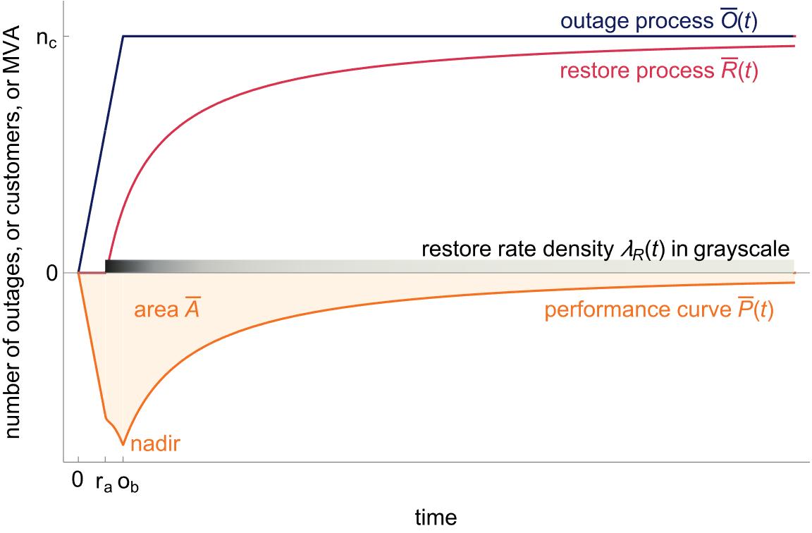
Figure 1: Mean processes for a resilience event with constant rate outages in $[0,o_{n}]$ and restores for $t\geq r_{a}$ at a slowing, lognormal rate $\lambda_{R}(t)$. The vertical axis lists three different quantities that can be used to track the event processes. Some of the parameters used are not typical to allow room for labeling; see Fig. 2 for a typical example.

The mean cumulative number of outages and the mean cumulative number of restores at time $t$ are

$$\mkern 3.0mu\overline{\mkern-3.0muO\mkern 0.0mu}\mkern 0.0mu(t)=\int_{0}^{t}\lambda_{O}(\tau)d\tau\mbox{ and }\mkern 3.0mu\overline{\mkern-3.0muR\mkern 0.0mu}\mkern 0.0mu(t)=\int_{0}^{t}\lambda_{R}(\tau)d\tau$$ (1)

The mean outage and restore rates $\lambda_{O}(t)$, $\lambda_{R}(t)$ and mean cumulative outages and restores $\mkern 3.0mu\overline{\mkern-3.0muO\mkern 0.0mu}\mkern 0.0mu(t)$, $\mkern 3.0mu\overline{\mkern-3.0muR\mkern 0.0mu}\mkern 0.0mu(t)$ easily generalize to track outages and restores of other quantities such as customers in a distribution system [5] or MVA ratings of lines in a transmission system [7]. For example, $\lambda_{O}(t)$ can be the mean rate at which customers outage and $\mkern 3.0mu\overline{\mkern-3.0muO\mkern 0.0mu}\mkern 0.0mu(t)$ can be the mean cumulative customers outaged. These choices change the vertical axis on which $\mkern 3.0mu\overline{\mkern-3.0muO\mkern 0.0mu}\mkern 0.0mu(t)$, $\mkern 3.0mu\overline{\mkern-3.0muR\mkern 0.0mu}\mkern 0.0mu(t)$, $\mkern 3.0mu\overline{\mkern-3.0muP\mkern 0.0mu}\mkern 0.0mu(t)$ are plotted. The mean performance curve $\mkern 3.0mu\overline{\mkern-3.0muP\mkern 0.0mu}\mkern 0.0mu(t)$ is the negative of the mean unrestored amount of the quantity tracked:

$$\mkern 3.0mu\overline{\mkern-3.0muP\mkern 0.0mu}\mkern 0.0mu(t)=\mkern 3.0mu\overline{\mkern-3.0muR\mkern 0.0mu}\mkern 0.0mu(t)-\mkern 3.0mu\overline{\mkern-3.0muO\mkern 0.0mu}\mkern 0.0mu(t)$$ (2)

At the start of the event, time $t=0$ and $\mkern 3.0mu\overline{\mkern-3.0muP\mkern 0.0mu}\mkern 0.0mu(0)=0$. $\mkern 3.0mu\overline{\mkern-3.0muP\mkern 0.0mu}\mkern 0.0mu(t)$ becomes negative during the event as shown in Fig. 1. Eventually, at time $\infty$, all the outages are restored, $\mkern 3.0mu\overline{\mkern-3.0muP\mkern 0.0mu}\mkern 0.0mu(\infty)=0$ and $\mkern 3.0mu\overline{\mkern-3.0muO\mkern 0.0mu}\mkern 0.0mu(\infty)=\mkern 3.0mu\overline{\mkern-3.0muR\mkern 0.0mu}\mkern 0.0mu(\infty)=n_{c}$. Depending on which quantity is tracked, $n_{c}$ is the total number of outages $n$, the total number of customers outaged, or the total MVA of lines outaged. Since $n_{c}=\mkern 3.0mu\overline{\mkern-3.0muO\mkern 0.0mu}\mkern 0.0mu(\infty)=\int_{0}^{\infty}\lambda_{O}(\tau)d\tau=\mkern 3.0mu\overline{\mkern-3.0muR\mkern 0.0mu}\mkern 0.0mu(\infty)=\int_{0}^{\infty}\lambda_{R}(\tau)d\tau$, $f_{o}(t)=\lambda_{O}(t)/n_{c}$ and $f_{r}(t)=\lambda_{R}(t)/n_{c}$ integrate to one, and are probability distributions of the outage times and restore times respectively. Write $\overline{o}=\int_{0}^{\infty}\tau f_{o}(\tau)d\tau$ for the mean outage time and $\overline{r}=\int_{0}^{\infty}\tau f_{r}(\tau)d\tau$ for the mean restore time.

II Area and nadir metrics

This section starts by giving general formulas for the area of the mean performance curve. This area (regarded as a positive area by including the minus sign) is

$$\mkern 3.0mu\overline{\mkern-3.0muA\mkern 0.0mu}\mkern 0.0mu=-\int_{0}^{\infty}\mkern 3.0mu\overline{\mkern-3.0muP\mkern 0.0mu}\mkern 0.0mu(t)dt=\int_{0}^{\infty}[\mkern 3.0mu\overline{\mkern-3.0muO\mkern 0.0mu}\mkern 0.0mu(t)-\mkern 3.0mu\overline{\mkern-3.0muR\mkern 0.0mu}\mkern 0.0mu(t)]dt$$ (3)

Moreover, $\mkern 3.0mu\overline{\mkern-3.0muA\mkern 0.0mu}\mkern 0.0mu$ is also the mean of the area $A$ of the performance curve $P(t)$, since

$$\mkern 3.0mu\overline{\mkern-3.0muA\mkern 0.0mu}\mkern 0.0mu=-\int_{0}^{\infty}{\rm E}P(t)dt=-{\rm E}\int_{0}^{\infty}P(t)dt={\rm E}A$$ (4)

Integrating (3) by parts, and using $\mkern 3.0mu\overline{\mkern-3.0muP\mkern 0.0mu}\mkern 0.0mu(0)=\mkern 3.0mu\overline{\mkern-3.0muP\mkern 0.0mu}\mkern 0.0mu(\infty)=0$ and $\lambda_{O}(t)=\mkern 3.0mu\overline{\mkern-3.0muO^{\prime}\!\mkern 0.0mu}\mkern 0.0mu(t)$, $\lambda_{R}(t)=\mkern 3.0mu\overline{\mkern-3.0muR^{\prime}\!\mkern 0.0mu}\mkern 0.0mu(t)$ gives the very nice formulas

$$\mkern 3.0mu\overline{\mkern-3.0muA\mkern 0.0mu}\mkern 0.0mu =\!-\!\int_{0}^{\infty}t{\mkern 3.0mu\overline{\mkern-3.0muP\mkern 0.0mu}\mkern 0.0mu^{\prime}\!}(t)dt=\int_{0}^{\infty}[t\lambda_{R}(t)-t\lambda_{O}(t)]dt={\rm E}[\lambda_{R}]-{\rm E}[\lambda_{O}]$$

$$=n_{c}\int_{0}^{\infty}[tf_{r}(t)-tf_{o}(t)]dt=n_{c}(\overline{r}-\overline{o})$$ (5)

According to (3), $\mkern 3.0mu\overline{\mkern-3.0muA\mkern 0.0mu}\mkern 0.0mu$ is also the area between the mean outage and mean restore processes (see Fig. 2), so that (5) can be understood as the height $n_{c}$ of this area times its average width.

This section now defines the nadir and observes where it occurs. The nadir $\mkern 3.0mu\overline{\mkern-3.0muN\mkern 0.0mu}\mkern 0.0mu$ of $\mkern 3.0mu\overline{\mkern-3.0muP\mkern 0.0mu}\mkern 0.0mu(t)$ is the maximum mean number of elements simultaneously outaged during the event, or the negative of the minimum value of $\mkern 3.0mu\overline{\mkern-3.0muP\mkern 0.0mu}\mkern 0.0mu(t)$:

$$\mkern 3.0mu\overline{\mkern-3.0muN\mkern 0.0mu}\mkern 0.0mu=-\min\{\mkern 3.0mu\overline{\mkern-3.0muP\mkern 0.0mu}\mkern 0.0mu(t),\ t\geq 0\}$$ (6)

Simulations and frameworks of resilience [1, 2, 3] often make the idealization that outages end before the restores start so that $r_{a}\geq o_{b}$. Then $\mkern 3.0mu\overline{\mkern-3.0muP\mkern 0.0mu}\mkern 0.0mu(t)$ is decreasing for $t<o_{b}$, constant in $[o_{b},r_{a}]$, and increasing for $t>r_{a}$. Therefore the nadir occurs at all the times in $[o_{b},r_{a}]$ and is simply $\mkern 3.0mu\overline{\mkern-3.0muN\mkern 0.0mu}\mkern 0.0mu=n_{c}$. For example, when $\mkern 3.0mu\overline{\mkern-3.0muP\mkern 0.0mu}\mkern 0.0mu(t)$ is a trapezoid, the nadir occurs along the bottom of the trapezoid. However, in real data [6, 5, 4, 7] the restores usually start before the end of the outages. Accordingly, the next paragraph and section III assume that $r_{a}<o_{b}$.

Since $\mkern 3.0mu\overline{\mkern-3.0muR\mkern 0.0mu}\mkern 0.0mu(t)=0$ and $\mkern 3.0mu\overline{\mkern-3.0muO\mkern 0.0mu}\mkern 0.0mu(t)$ is increasing for $t<r_{a}$, and $\mkern 3.0mu\overline{\mkern-3.0muO\mkern 0.0mu}\mkern 0.0mu(t)=n_{c}$ and $\mkern 3.0mu\overline{\mkern-3.0muR\mkern 0.0mu}\mkern 0.0mu(t)$ is increasing for $t>o_{b}$, the nadir $\mkern 3.0mu\overline{\mkern-3.0muN\mkern 0.0mu}\mkern 0.0mu$ of $\mkern 3.0mu\overline{\mkern-3.0muP\mkern 0.0mu}\mkern 0.0mu(t)=\mkern 3.0mu\overline{\mkern-3.0muR\mkern 0.0mu}\mkern 0.0mu(t)-\mkern 3.0mu\overline{\mkern-3.0muO\mkern 0.0mu}\mkern 0.0mu(t)$ must occur inside the time interval $[r_{a},o_{b}]$ or at its endpoints. $\mkern 3.0mu\overline{\mkern-3.0muP\mkern 0.0mu}\mkern 0.0mu(t)$ is a smooth function in $[r_{a},o_{b}]$.

III Metric formulas for different cases

III-A Constant rate outage and restore processes

The simplest model has outage and restore processes with constant rates $\lambda_{O}$ and $\lambda_{R}$ respectively. Then

$$\!\!\lambda_{O} =\frac{n_{c}}{o_{b}}\mbox{ and }\mkern 3.0mu\overline{\mkern-3.0muO\mkern 0.0mu}\mkern 0.0mu(t)=\lambda_{O}t,\ 0\leq t<o_{b}$$ (7)

$$\!\!\lambda_{R} =\frac{n_{c}}{r_{b}-r_{a}}\mbox{ and }\mkern 3.0mu\overline{\mkern-3.0muR\mkern 0.0mu}\mkern 0.0mu(t)=\lambda_{R}(t-r_{a}),\ r_{a}\leq t\leq r_{b}$$ (8)

The mean area $\mkern 3.0mu\overline{\mkern-3.0muA\mkern 0.0mu}\mkern 0.0mu$ is obtained using (5) with the mean restore time $\overline{r}=\tfrac{1}{2}(r_{a}+r_{b})$ and mean outage time $\overline{o}=\tfrac{1}{2}o_{b}$:

$$\mkern 3.0mu\overline{\mkern-3.0muA\mkern 0.0mu}\mkern 0.0mu =n_{c}\,(\tfrac{1}{2}(r_{a}+r_{b})-\tfrac{1}{2}o_{b})$$ (9)

To compute the nadir $\mkern 3.0mu\overline{\mkern-3.0muN\mkern 0.0mu}\mkern 0.0mu$, which always occurs in $[r_{a},o_{b}]$, note that $\mkern 3.0mu\overline{\mkern-3.0muP^{\prime}\!\mkern 0.0mu}\mkern 0.0mu(t)=\lambda_{R}-\lambda_{O}$ in $[r_{a},o_{b}]$. Therefore, if $\lambda_{R}>\lambda_{O}$ then $\mkern 3.0mu\overline{\mkern-3.0muP^{\prime}\!\mkern 0.0mu}\mkern 0.0mu(t)>0$ and $\mkern 3.0mu\overline{\mkern-3.0muN\mkern 0.0mu}\mkern 0.0mu=\lambda_{O}r_{a}=n_{c}r_{a}/o_{b}$ occurs at time $r_{a}$. Or if $\lambda_{R}<\lambda_{O}$ then $\mkern 3.0mu\overline{\mkern-3.0muP^{\prime}\!\mkern 0.0mu}\mkern 0.0mu(t)<0$ and $\mkern 3.0mu\overline{\mkern-3.0muN\mkern 0.0mu}\mkern 0.0mu=n_{c}-\lambda_{R}(o_{b}-r_{a})=n_{c}(r_{b}-o_{b})/(r_{b}-r_{a})$ occurs at time $o_{b}$.

The restore duration can be measured by $\mkern 3.0mu\overline{\mkern-3.0muD\mkern 0.0mu}\mkern 0.0mu_{n}=r_{b}-r_{a}$.

III-B Lognormal rate restore process

Consider the case of constant rate outage process (7) and restore process $\lambda_{R}(t)$ proportional to lognormal with parameters $\mu$ and $\sigma$ that is used to model typical North American transmission events in [4], so that $\lambda_{R}(t)=n_{c}f_{r}(t)$ has

$$f_{r}(t) =((t-r_{a})\sigma\sqrt{2\pi})^{-1}\exp[-(\ln(t-r_{a})-\mu)^{2}/(2\sigma^{2})]$$

$$\mkern 3.0mu\overline{\mkern-3.0muR\mkern 0.0mu}\mkern 0.0mu(t) =n_{c}\,\Phi[(\ln(t-r_{a})-\mu)/\sigma],\qquad\qquad t\geq r_{a}$$ (10)

$\Phi$ is the CDF of the standard normal distribution. The lognormal distribution $f_{r}(t)$ in (10) has mean $\overline{r}=r_{a}+\exp[\mu+\sigma^{2}/2]$ and the area (5) becomes

$$\mkern 3.0mu\overline{\mkern-3.0muA\mkern 0.0mu}\mkern 0.0mu =n_{c}\,(r_{a}+e^{\mu+\sigma^{2}/2}-o_{b}/2)$$ (11)

To compute the nadir, which is in $[r_{a},o_{b}]$, note that the CDF of the lognormal distribution and hence $\mkern 3.0mu\overline{\mkern-3.0muR\mkern 0.0mu}\mkern 0.0mu(t)$ and $\mkern 3.0mu\overline{\mkern-3.0muP\mkern 0.0mu}\mkern 0.0mu(t)$ are convex in $[r_{a},t_{\rm inflect}]$ and concave for $t\geq t_{\rm inflect}$, where $t_{\rm inflect}=e^{\mu-\sigma^{2}}+r_{a}$ is the mode (maximum) of the lognormal distribution for which $\mkern 3.0mu\overline{\mkern-3.0muR^{\prime\prime}\!\!\!\mkern 0.0mu}\mkern 0.0mu\,\,(t_{\rm inflect})=\mkern 3.0mu\overline{\mkern-3.0muP^{\prime\prime}\!\!\!\mkern 0.0mu}\mkern 0.0mu\,\,(t_{\rm inflect})=0$. Then

$$\mkern 3.0mu\overline{\mkern-3.0muP^{\prime}\!\mkern 0.0mu}\mkern 0.0mu(t_{\rm inflect}) =n_{c}(\sigma\sqrt{2\pi})^{-1}\exp[-\mu+\sigma^{2}/2]-n_{c}/o_{b}$$ (12)

Write $t_{*}$ for a local minimum of $\mkern 3.0mu\overline{\mkern-3.0muP\mkern 0.0mu}\mkern 0.0mu(t)$. Then $0=\mkern 3.0mu\overline{\mkern-3.0muP^{\prime}\!\mkern 0.0mu}\mkern 0.0mu(t_{*})=n_{c}f_{r}(t_{*})-n_{c}/o_{b}$, and some algebra yields a quadratic equation $[\ln(t_{*}-r_{a})]^{2}+2(\sigma^{2}-\mu)[\ln(t_{*}-r_{a})]+\mu^{2}+2\sigma^{2}\ln[\sigma\smash{\sqrt{2\pi}/o_{b}}]=0$ that can be solved to give

$$t_{*} =r_{a}+\exp\!\big{[}\mu-\sigma^{2}-\sigma\sqrt{\sigma^{2}-2\mu-2\ln[\sigma\sqrt{2\pi}/o_{b}]}\,\big{]}$$ (13)

$$=r_{a}+\exp\!\big{[}\mu-\sigma^{2}-\sigma\sqrt{2\ln[1\!+\!(o_{b}/n_{c})\mkern 3.0mu\overline{\mkern-3.0muP^{\prime}\!\mkern 0.0mu}\mkern 0.0mu(t_{\rm inflect})]}\,\big{]}$$ (14)

The negative sign for the square root in (13) is chosen to obtain the solution in the convex part of $\mkern 3.0mu\overline{\mkern-3.0muP\mkern 0.0mu}\mkern 0.0mu(t)$ that can be the minimum. A real solution for $t_{*}$ exists if $\mkern 3.0mu\overline{\mkern-3.0muP^{\prime}\!\mkern 0.0mu}\mkern 0.0mu(t_{\rm inflect})\geq 0$.

If $t_{\rm inflect}\leq o_{b}$, then $\mkern 3.0mu\overline{\mkern-3.0muP^{\prime}\!\mkern 0.0mu}\mkern 0.0mu(r_{a})=-\lambda_{O}<0$ and $\mkern 3.0mu\overline{\mkern-3.0muP^{\prime\prime}\!\!\!\mkern 0.0mu}\mkern 0.0mu\,\,(t)\geq 0$ in $[r_{a},t_{\rm inflect}]$ due to convexity. If $\mkern 3.0mu\overline{\mkern-3.0muP^{\prime}\!\mkern 0.0mu}\mkern 0.0mu(t_{\rm inflect})\leq 0$, then, since $\mkern 3.0mu\overline{\mkern-3.0muP^{\prime\prime}\!\!\!\mkern 0.0mu}\mkern 0.0mu\,\,(t)\leq 0$ in $[t_{\rm inflect},o_{b}]$, $\mkern 3.0mu\overline{\mkern-3.0muP^{\prime}\!\mkern 0.0mu}\mkern 0.0mu(t)\leq 0$ in $[r_{a},o_{b}]$ and the nadir occurs at $o_{b}$. If $\mkern 3.0mu\overline{\mkern-3.0muP^{\prime}\!\mkern 0.0mu}\mkern 0.0mu(t_{\rm inflect})>0$, the minimum of $\mkern 3.0mu\overline{\mkern-3.0muP\mkern 0.0mu}\mkern 0.0mu(t)$ in $[r_{a},t_{\rm inflect}]$ occurs at $t_{*}$ and does not occur at $t_{\rm inflect}$. Since $\mkern 3.0mu\overline{\mkern-3.0muP^{\prime\prime}\!\!\!\mkern 0.0mu}\mkern 0.0mu\,\,(t)\leq 0$ in $[t_{\rm inflect},o_{b}]$, the minimum of $\mkern 3.0mu\overline{\mkern-3.0muP\mkern 0.0mu}\mkern 0.0mu(t)$ in $[t_{\rm inflect},o_{b}]$ could occur at $o_{b}$. So the nadir occurs at $t_{*}$ or $o_{b}$.

If $t_{\rm inflect}>o_{b}$, then reasoning on $[r_{a},o_{b}]$ similar to the reasoning for $t_{\rm inflect}<o_{b}$ on $[r_{a},t_{\rm inflect}]$ shows that if $\mkern 3.0mu\overline{\mkern-3.0muP^{\prime}\!\mkern 0.0mu}\mkern 0.0mu(o_{b})\leq 0$, the nadir occurs at $o_{b}$, and if $\mkern 3.0mu\overline{\mkern-3.0muP^{\prime}\!\mkern 0.0mu}\mkern 0.0mu(o_{b})>0$, the nadir occurs at $t_{*}$.

One concludes that the nadir occurs at $t_{*}$ (if it exists in $[r_{a},o_{b}]$) or at $o_{b}$ so that $\mkern 3.0mu\overline{\mkern-3.0muN\mkern 0.0mu}\mkern 0.0mu=-\min\{P(t_{*}),P(o_{b})\}$.

The duration to reach 95% restoration can be measured by $\mkern 3.0mu\overline{\mkern-3.0muD\mkern 0.0mu}\mkern 0.0mu_{95\%}^{\rm ln}={\rm exp}[\mu+\sigma\,\Phi^{-1}(0.95)]$. The geometric mean and median of the positive restore times relative to $r_{a}$ is $\mkern 3.0mu\overline{\mkern-3.0muD\mkern 0.0mu}\mkern 0.0mu_{\rm GM}=e^{\mu}$ [4].

III-C Exponential rate restore process

Another case is exponential recovery with time constant and mean restore time $\tau$:

$$f_{r}(t) =\tau^{-1}\,e^{-(t-r_{a})/\tau}$$

$$\mkern 3.0mu\overline{\mkern-3.0muR\mkern 0.0mu}\mkern 0.0mu(t) =n_{c}[1-e^{-(t-r_{a})/\tau}],\quad t\geq r_{a}$$ (15)

The area (5) becomes

$$\mkern 3.0mu\overline{\mkern-3.0muA\mkern 0.0mu}\mkern 0.0mu =n_{c}\,(r_{a}+\tau-o_{b}/2)$$ (16)

$\mkern 3.0mu\overline{\mkern-3.0muR\mkern 0.0mu}\mkern 0.0mu(t)$ is concave, so the nadir occurs at either $r_{a}$ or $o_{b}$ and is $\mkern 3.0mu\overline{\mkern-3.0muN\mkern 0.0mu}\mkern 0.0mu=-\min\{-\lambda_{O}r_{a},n_{c}[1-e^{-(o_{b}-r_{a})/\tau}]-\lambda_{O}o_{b}\}$ $=n_{c}\max\{r_{a}/o_{b},e^{-(o_{b}-r_{a})/\tau}\}$.

The duration to reach 95% restoration is $\mkern 3.0mu\overline{\mkern-3.0muD\mkern 0.0mu}\mkern 0.0mu_{95\%}^{\rm exp}=\tau\ln 20$.

IV Area $A$ for empirical data

Similar methods apply to analyzing the data recorded from an actual event, except that $O(t)$, $R(t)$, $P(t)$ are now actual instead of their means. This section analyzes the area $A$ of $P(t)$. Suppose the outages occur at times $o_{1}\leq...\leq o_{n}$, with quantities $c_{1},...,c_{n}$. Restores occur at $r_{1}\leq...\leq r_{n}$, with quantities $c_{\pi(1)},...,c_{\pi(n)}$, where $\pi$ is the permutation of $1,2,...,n$ indicating the order in which the outages restore. The restores in the order of their outage are $r_{\pi^{-1}(1)},...,r_{\pi^{-1}(n)}$ where $\pi^{-1}$ is the inverse permutation.

The rates are proportional to delta functions at the outage and restore times, and $O(t)$ and $R(t)$ become step functions:

$$\lambda_{O}(t) =\sum_{i=1}^{n}c_{i}\delta(t-o_{i})\mbox{ and }O(t)=\sum_{k:o_{k}\leq t}c_{k}$$ (17)

$$\lambda_{R}(t) =\sum_{i=1}^{n}c_{\pi(i)}\delta(t-r_{i})\mbox{ and }R(t)=\sum_{k:r_{k}\leq t}c_{\pi(k)}$$ (18)

$$\mbox{Then }\ A ={\rm E}[\lambda_{R}]-{\rm E}[\lambda_{O}]=\sum_{i=1}^{n}(c_{\pi(i)}r_{i}-c_{i}o_{i})$$ (19)

Note that permuting the order of the restores in the sum in (19) makes no difference. Therefore if one writes $\rho_{i}=r_{\pi^{-1}(i)}-o_{i}$ for the time to restore or repair outage $i$, one obtains

$$A =\sum_{i=1}^{n}c_{i}(r_{\pi^{-1}(i)}-o_{i})=\sum_{i=1}^{n}c_{i}\rho_{i}$$ (20)

A restricted but useful case is now analyzed: Write $A_{x}$ for the area when $c_{1}=c_{2}=...=c_{n}=x$ where $x$ is a constant. For example, $A_{1}$ is the area of the performance curve when it tracks the number of outages, and $A_{\overline{c}}$ is the area of the performance curve when it tracks the number of customers out and one makes the approximation that the average number of customers $\overline{c}=n_{c}/n$ is out at each outage so that $c_{i}=\overline{c}$. Equations (19) and (20) reduce to

$$A_{\overline{c}} ={\overline{c}}\sum_{i=1}^{n}(r_{i}-o_{i})=n\overline{c}(\overline{r}-\overline{o})=n_{c}(\overline{r}-\overline{o})=n_{c}\,\mkern 3.0mu\overline{\mkern-3.0mu\rho\mkern 0.0mu}\mkern 0.0mu$$ (21)

where $\mkern 3.0mu\overline{\mkern-3.0mu\rho\mkern 0.0mu}\mkern 0.0mu$ is the mean time to repair in the event. Equation (21) recovers the useful (5) for empirical data in the case that the quantities outaged are interchangeable, including $A_{1}$.

Another approach [5] assumes $c_{1},c_{2},...,c_{n}$ are sampled from a random variable independent of the outage and restore times with mean $\overline{c}$. Then taking the expectation of (20) gives

$$\mkern 3.0mu\overline{\mkern-3.0muA\mkern 0.0mu}\mkern 0.0mu={\rm E}A=\sum_{i=1}^{n}{\rm E}c_{i}{\rm E}[r_{\pi^{-1}(i)}-o_{i}]=n\overline{c}(\overline{r}-\overline{o})=n\overline{c}\,\overline{\rho}$$ (22)

V Typical resilience event example

This section shows a typical North American transmission resilience event in Fig. 2 based on data from [4]. The event is typical in the class of resilience events with at least 10 outages in the bulk electric power system operated at 100 kV and higher across the continental USA and Canada from 2015 to 2021. The outage data is collected by the North American Electric Reliability Corporation (NERC) in their Transmission Availability Data System (TADS). Some applications would usefully consider the events typical for subsets of data such as events with specific causes such as hurricanes or winter storms, or events in particular seasons or regions, but this example considers all the data. Fig. 2 uses the median parameters for these event data from [4]: number of outages $n=13.5$, which is rounded up to $n=14$, outage duration $o_{b}=2.69$ h, time to first restore $r_{a}=0.52$ h, and lognormal distribution restoration parameters $\mu=1.64$ and $\sigma=1.56$ ($\mu=\ln{D_{\rm GM}}$ is calculated with $D_{\rm GM}=5.15$ h).

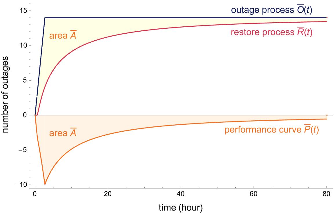
Figure 2: Typical North American transmission system resilience event tracked by number of outages on the vertical scale. The shaded area $\mkern 3.0mu\overline{\mkern-3.0muA\mkern 0.0mu}\mkern 0.0mu$ of $\mkern 3.0mu\overline{\mkern-3.0muP\mkern 0.0mu}\mkern 0.0mu(t)$ is the same as the shaded area between $\mkern 3.0mu\overline{\mkern-3.0muO\mkern 0.0mu}\mkern 0.0mu(t)$ and $\mkern 3.0mu\overline{\mkern-3.0muR\mkern 0.0mu}\mkern 0.0mu(t)$.

VI Discussion and conclusions

This letter introduces Poisson process models in terms of their rates for outage and restore resilience processes (7,8,10,15) and performance curves (2). The model parameters can be calculated from standard utility outage data [4]. One of the parameters $n_{c}$ is the event total of the quantity tracked by the processes, such as number of outages, or number of customers, or MVA rating of the lines. Section III gives explicit formulas in terms of the parameters for area, nadir, and duration metrics describing the mean performance curve $\mkern 3.0mu\overline{\mkern-3.0muP\mkern 0.0mu}\mkern 0.0mu(t)$ for a constant rate outage process and constant, lognormal, or exponential rate restore processes. In each case, the restore duration has a different definition and formula, and the event duration is always the restore duration plus the time to the first restore $r_{a}$. In all these cases, the nadir of $\mkern 3.0mu\overline{\mkern-3.0muP\mkern 0.0mu}\mkern 0.0mu(t)$ is proportional to $n_{c}$ and occurs only at the end of the outages $o_{b}$ or at another time that can be explicitly calculated. Then the nadir is calculated as the minimum of $\mkern 3.0mu\overline{\mkern-3.0muP\mkern 0.0mu}\mkern 0.0mu(t)$ at the two times. Moreover, for the North American transmission events in [4], 98% of the nadirs occur at the end of the outages so that $\mkern 3.0mu\overline{\mkern-3.0muN\mkern 0.0mu}\mkern 0.0mu=-\mkern 3.0mu\overline{\mkern-3.0muP\mkern 0.0mu}\mkern 0.0mu(o_{b})$.

$\mkern 3.0mu\overline{\mkern-3.0muA\mkern 0.0mu}\mkern 0.0mu$ is area of the mean performance curve, area between the mean outage and restore processes, and expected area of the performance curve. $\mkern 3.0mu\overline{\mkern-3.0muA\mkern 0.0mu}\mkern 0.0mu$ is given by (5,9,11,16) as the difference between the average restore and outage rates, or $n_{c}$ times the difference between the average restore and outage times. Thus 10% reduction in $n_{c}$ causes the same 10% reduction of $\mkern 3.0mu\overline{\mkern-3.0muA\mkern 0.0mu}\mkern 0.0mu$ as 10% faster restoration.

The area $A$ of the performance curve for empirical data is also the difference between average restore and outage rates (19), and is expressed in terms of component repair times in (20), which, in the case of interchangeable outages such as when counting the number of outages, simplifies to $n_{c}$ times the average repair time in (21). This links the outage and restore process systems view with the individual component reliability view.

Areas of performance curves or mean performance curves represent component hours, customer hours, or MVA hours in a resilience event, and the usefulness of these metrics underlines the importance of giving new derivations for intuitive formulas showing how the areas depend on $n_{c}$ and average outage, restore, and repair times.

References

• [1] A. Stanković, K. Tomsovic et al., Methods for analysis and quantification of power system resilience, IEEE Trans. Power Systems, 2022, doi: 10.1109/TPWRS.2022.3212688.
• [2] M. Panteli, D. N. Trakas, P. Mancarella, N. D. Hatziargyriou, Power systems resilience assessment: hardening and smart operational enhancement, Proceedings IEEE, vol. 105, no. 7, July 2017, pp. 1202-1213.
• [3] C. Nan, G. Sansavini, A quantitative method for assessing resilience of interdependent infrastructures, Reliability Engineering & System Safety, vol. 157, Jan. 2017, pp. 35-53.
• [4] I. Dobson, S. Ekisheva, How long is a resilience event in a transmission system?: Metrics and models driven by utility data, IEEE Trans. Power Systems, accepted July 2023, doi: 10.1109/TPWRS.2023.3292328.
• [5] N.K. Carrington I. Dobson, Z. Wang, Extracting resilience metrics from distribution utility data using outage and restore process statistics, IEEE Trans. Power Systems, vol. 36, no. 2, Nov. 2021, pp. 5814-5823.
• [6] Y. Wei, C. Ji, F. Galvan, S. Couvillon, G. Orellana, J. Momoh, Non-stationary random process for large-scale failure and recovery of power distribution, Applied Mathematics, vol. 7, no. 3, 2016, pp. 233-249.
• [7] S. Ekisheva, I. Dobson, J. Norris, R. Rieder, Assessing transmission resilience during extreme weather with outage and restore processes, Probability Methods Applied to Power Systems, Manchester UK, June 2022.