Smoothness properties of principal angles between subspaces
with applications to angular values of dynamical systems

Abstract

In this work we provide detailed estimates of maximal principal angles between subspaces and we analyze their smoothness for smoothly varying subspaces. This leads to a new definition of angular values for linear dynamical systems in continuous time. We derive some of their properties complementary to the theory of angular values developed in [4], [5] for discrete time systems. The estimates are further employed to establish upper semicontinuity of angular values for some parametric model examples of discrete and continuous type.

37C05, 37E45, 34D09, 65Q10.

1 Introduction

Principal angles between linear subspaces of a Euclidean space form a standard tool in numerical linear algebra which can be computed via a singular value decomposition ([6, 11], [13, Ch.6.4]). The maximal principal angle is a measure of the distance between two elements in the Grassmann manifold of all subspaces of a fixed dimension (it is indeed a metric; see Proposition 2.3). This motivates its usefulness for various areas of application, such as optimization [19] signal processing [12, 18], and finite element methods [17].

In two previous papers [4, 5] the authors (in [4] jointly with G. Froyland) introduced the new notion of angular values for subspaces of arbitrary dimensions in a linear time discrete dynamical system. In essence, the angular value of dimension $s$ measures the maximal average rotation in terms of principal angles which an arbitrary subspace of dimension $s$ experiences through the dynamics of the given system. In the discrete time setting, it turned out that precise estimates and continuity properties are essential for deriving reduction theorems [5, Section 3] and explicit formulas for autonomous systems [4, Section 5,6]. In particular, the algorithm set up in [5, Section 4] is based on principal angles and the reduction principle.

The first goal of this paper is to sharpen Lipschitz estimates of the maximal principal angle and to show its smoothness when the underlying subspace moves smoothly with respect to a parameter; see Lemma 3.4 and Theorem 3.7. Let us note that this particular derivative can be obtained without any assumption on the leading singular value or on higher regularity. This is in contrast to the general problem of smooth singular values which has been studied extensively in the literature; see [7, 9, 10].

In Section 4 we use the formula for the derivative to define angular values of $4$ types for nonautonomous linear systems in continuous time. Then we investigate the invariance of angular values under asymptotically constant kinematic transformations (Propositions 4.3 and 4.8) in both discrete and continuous time. In the continuous autonomous case this allows us to reduce the computation of angular values to systems with matrices in real quasitriangular Schur form. If the Schur form contains several $2\times 2$ blocks with complex eigenvalues then the explicit formula (see Proposition 4.19) leads to an integral expression which relies on the rational independence of the frequencies and which involves Birkhoff’s ergodic theorem (see e.g. [2, Theorem 2.2]).

Finally, we consider the perturbation sensitivity of angular values, in particular continuity with respect to parameters. In [4, eq.(6.8)] we found the surprising fact that lower semicontinuity fails for angular values in general, even for a discrete autonomous system with a parameter dependent $2\times 2$-matrix. Nevertheless, we show that upper semicontinuity holds for this example which solves an open problem from [4, Outlook]. Moreover, we prove in Section 4.4 that upper semicontinuity holds for a continuous time system with a $4\times 4$-matrix which has two complex eigenvalues. In this case critical points where lower semicontinuity fails are determined by rational ratios of both frequencies.

2 Principal angles and metrics on the Grassmannian

In this section we collect basic properties of principal angles between subspaces. We show that the maximal principal angle provides a metric on the Grassmannian and compare it with other common metrics. Moreover, we study the invariance of principal angles under linear transformations.

2.1 Definition of principal angles and elementary properties

The following definition is taken from [13, Ch.6.4.3].

Definition 2.1

Let $V,W$ be subspaces of $\mathbbm{R}^{d}$ of dimension $s$. Then the principal angles $0\leq\phi_{1}\leq\ldots\leq\phi_{s}\leq\frac{\pi}{2}$ and associated principal vectors $v_{j}\in V$, $w_{j}\in W$ are defined recursively for $j=1,\ldots,s$ by

$$\cos(\phi_{j})=\max_{\begin{subarray}{c}v\in V,\|v\|=1\\ v^{\top}v_{\ell}=0,\ell=1,\ldots,j-1\end{subarray}}\ \max_{\begin{subarray}{c}w\in W,\|w\|=1\\ w^{\top}w_{\ell}=0,\ell=1,\ldots,j-1\end{subarray}}v^{\top}w=v_{j}^{\top}w_{j}.$$

We write $\measuredangle(V,W)=\phi_{s}$ for the largest principal angle and in case $s=1$ set $\measuredangle(v,w):=\measuredangle(\mathrm{span}(v),\mathrm{span}(w))$ for $v,w\in\mathbbm{R}^{d}$, $v,w\neq 0$. Further, recall from [4, Prop.2.3] an alternative variational characterization and from [13, Ch.6.4.3] an algorithm for computing principal angles via singular values.

Proposition 2.2

Let $V,W\subseteq\mathbbm{R}^{d}$ be two $s$-dimensional subspaces.

• The principal angles and principal vectors satisfy for $j=s,\ldots,1$

  $$\cos(\phi_{j})=\min_{\begin{subarray}{c}v\in V,\|v\|=1\\ v^{\top}v_{\ell}=0,\ell=j+1,\ldots,s\end{subarray}}\ \max_{\begin{subarray}{c}w\in W,\|w\|=1\\ w^{\top}w_{\ell}=0,\ell=j+1,\ldots,s\end{subarray}}v^{\top}w=v_{j}^{\top}w_{j}.$$

  In particular, the following max-min principle holds

  (1) $$\measuredangle(V,W)=\max_{\begin{subarray}{c}v\in V\\ v\neq 0\end{subarray}}\min_{\begin{subarray}{c}w\in W\\ w\neq 0\end{subarray}}\measuredangle(v,w)=\arccos\big{(}\min_{\begin{subarray}{c}v\in V\\ \|v\|=1\end{subarray}}\max_{\begin{subarray}{c}w\in W\\ \|w\|=1\end{subarray}}v^{\top}w\big{)}.$$

• Choose $P,Q\in\mathbbm{R}^{d,s}$ such that $P^{\top}P=Q^{\top}Q=I_{s}$, $V=\mathcal{R}(P)$, $W=\mathcal{R}(Q)$ and consider the SVD

  (2) $$P^{\top}Q=Y\Sigma Z^{\top},\quad Y,Z,\Sigma=\mathrm{diag}(\sigma_{1},\ldots,\sigma_{s})\in\mathbbm{R}^{s,s},\quad Y^{\top}Y=I_{s}=Z^{\top}Z,$$

  where $\sigma_{1}\geq\cdots\geq\sigma_{s}>0$. Then the principal angles of $V$ and $W$ satisfy $\sigma_{j}=\cos(\phi_{j})$ for $j=1,\ldots,s$ with principal vectors given by

  $$PY=\begin{pmatrix}v_{1}&\cdots&v_{s}\end{pmatrix},\quad QZ=\begin{pmatrix}w_{1}&\cdots&w_{s}\end{pmatrix}.$$

2.2 Some metrics on the Grassmannian

In this section we consider the Grassmann manifold (see [13, Ch.6.4.3])

$$\mathcal{G}(s,d)=\{V\subseteq\mathbbm{R}^{d}\;\text{is a subspace of dimension}\;s\}$$

and study its various metrics.

Proposition 2.3

The Grassmannian $\mathcal{G}(s,d)$ is a compact smooth manifold of dimension $s(d-s)$. Two metrics on $\mathcal{G}(s,d)$ are given for $V,W\in\mathcal{G}(s,d)$ by

(3) $$d_{1}(V,W)=\measuredangle(V,W),\qquad d_{2}(V,W)=\|P_{V}-P_{W}\|,$$

where $P_{V},P_{W}$ are the orthogonal projections onto $V$ and $W$, respectively, and $\|\cdot\|$ is the spectral norm. Both metrics are equivalent and related for $V,W\in\mathcal{G}(s,d)$ by

(4) $$d_{2}(V,W) =\sin(\measuredangle(V,W)),$$

$$\frac{2}{\pi}\measuredangle(V,W) \leq d_{2}(V,W)\leq\measuredangle(V,W).$$

Proof 2.4

The results for the metric $d_{2}$ can be found in [13, Ch.2.5.3,6.4.3] with the estimate in (4) taken from [4, Prop.2.5]. The definiteness and symmetry of $d_{1}$ follow directly from Proposition 2.2 (ii). For the triangle inequality we quoted [15, Theorem 3] in [4, Prop.2.5], but realized that this reference uses an angle $\theta$ between subspaces related to principal angles by $\cos(\theta)=\cos(\phi_{1})\cdots\cos(\phi_{s})$; see [15, Theorem 5]. We did not find a reference to the triangle inequality for $d_{1}$ elsewhere, so we provide a proof here for completeness. Let us first consider the case $s=1$. Let $u,v,w\in\mathbbm{R}^{d}$ satisfy $\|u\|=\|v\|=\|w\|=1$ and let $B=\begin{pmatrix}u&w&v\end{pmatrix}\in\mathbbm{R}^{d,3}$, so that $\mathcal{R}(B)=\mathrm{span}(u,w,v)$. Further, by suitable sign changes of $v$ and $w$, we can arrange $u^{\top}v\geq 0$ and $u^{\top}w\geq 0$ (but not necessarily $v^{\top}w\geq 0$ !). Then take a short QR-decomposition of $B$ i.e.

$$B=QR,\quad Q\in\mathbbm{R}^{d,3},\ Q^{\top}Q=I_{3},\quad R=\begin{pmatrix}\tilde{u}&\tilde{w}&\tilde{v}\end{pmatrix}\in\mathbbm{R}^{3,3},$$

where $R$ is upper triangular and has nonnegative diagonal elements. Since $R^{\top}R=B^{\top}B$, all inner products are conserved and we can assume

$$\tilde{u}=\begin{pmatrix}1\\ 0\\ 0\end{pmatrix},\quad\tilde{w}=\begin{pmatrix}\cos(\alpha)\\ \sin(\alpha)\\ 0\end{pmatrix},\quad\tilde{v}=r\begin{pmatrix}\cos(\beta)\\ \sin(\beta)\\ 0\end{pmatrix}+\begin{pmatrix}0\\ 0\\ v_{3}\end{pmatrix},$$

where $0\leq\alpha\leq\frac{\pi}{2}$, $|\beta|\leq\frac{\pi}{2}$, $r\geq 0$, and $r^{2}+v_{3}^{2}=1$. Recall the relations $0\leq u^{\top}w=\tilde{u}^{\top}\tilde{w}=\cos(\alpha)$, $0\leq u^{\top}v=\tilde{u}^{\top}\tilde{v}=r\cos(\beta)$, and $0\leq R_{22}=\sin(\alpha)$. By the invariance of the angle under orthogonal transformations (cf. Section 2.3) we have

$$\measuredangle(u,v)=\measuredangle(\tilde{u},\tilde{v}),\quad\measuredangle(u,w)=\measuredangle(\tilde{u},\tilde{w}),\quad\measuredangle(w,v)=\measuredangle(\tilde{w},\tilde{v}).$$

Hence it suffices to prove

$$\measuredangle(\tilde{u},\tilde{w}) \leq\measuredangle(\tilde{u},\tilde{v})+\measuredangle(\tilde{v},\tilde{w}).$$

Since $0\leq r\leq 1$, $\cos(\beta)\geq 0$ and $\arccos$ is monotone decreasing we find

$$\measuredangle(\tilde{u},\tilde{w}) =\alpha,\quad\measuredangle(\tilde{u},\tilde{v})=\arccos(r\cos(\beta))\geq\arccos(\cos(\beta))=|\beta|.$$

The value of $\measuredangle(\tilde{v},\tilde{w})=\arccos(r|\cos(\alpha-\beta)|)$ depends on the sign of $\cos(\alpha-\beta)$, which is positive for $|\alpha-\beta|\leq\frac{\pi}{2}$ and negative otherwise. Since $\alpha-\beta\geq-\frac{\pi}{2}$ the second case occurs for $\frac{\pi}{2}<\alpha-\beta\leq\pi$ where we have $-\cos(\alpha-\beta)=\cos(\pi-(\alpha-\beta))$. Summarizing, we obtain

$$\measuredangle(\tilde{v},\tilde{w}) =\begin{cases}\arccos(r\cos(\alpha-\beta)),&|\alpha-\beta|\leq\frac{\pi}{2},\\ \arccos(r\cos(\pi-\alpha+\beta)),&\frac{\pi}{2}<\alpha-\beta,\end{cases}$$

$$\geq\begin{cases}|\alpha-\beta|,&|\alpha-\beta|\leq\frac{\pi}{2},\\ \pi-\alpha+\beta,&\beta<\alpha-\frac{\pi}{2}\leq 0.\end{cases}$$

We find in the first case

$$\measuredangle(\tilde{u},\tilde{w}) =\alpha\leq|\beta|+|\alpha-\beta|\leq\measuredangle(\tilde{u},\tilde{v})+\measuredangle(\tilde{v},\tilde{w})$$

and in the second case

$$\measuredangle(\tilde{u},\tilde{w}) =\alpha\leq\pi-\alpha=|\beta|+\pi-\alpha+\beta\leq\measuredangle(\tilde{u},\tilde{v})+\measuredangle(\tilde{v},\tilde{w}).$$

This proves the triangle inequality for $s=1$. For $s\geq 1$ we use the representation (1) from the max-min principle. For ease of notation we set $U_{0}=U\setminus\{0\}$, $V_{0}=V\setminus\{0\}$, $W_{0}=W\setminus\{0\}$. Using the estimate from case $s=1$ we conclude

$$\measuredangle(u,w) \leq\measuredangle(u,v)+\measuredangle(v,w),\quad\forall u\in U_{0},v\in V_{0},w\in W_{0},$$

$$\min_{w\in W_{0}}\measuredangle(u,w) \leq\measuredangle(u,v)+\min_{w\in W_{0}}\measuredangle(v,w),\quad\forall u\in U_{0},v\in V_{0},$$

$$\min_{w\in W_{0}}\measuredangle(u,w) \leq\min_{v\in V_{0}}\left[\measuredangle(u,v)+\min_{w\in W_{0}}\measuredangle(v,w)\right]$$

$$\leq\min_{v\in V_{0}}\measuredangle(u,v)+\max_{v\in V_{0}}\min_{w\in W_{0}}\measuredangle(v,w),\quad\forall u\in U_{0},$$

$$\max_{u\in U_{0}}\min_{w\in W_{0}}\measuredangle(u,w) \leq\max_{u\in U_{0}}\min_{v\in V_{0}}\measuredangle(u,v)+\max_{v\in V_{0}}\min_{w\in W_{0}}\measuredangle(v,w),$$

$$\measuredangle(U,W) \leq\measuredangle(U,V)+\measuredangle(V,W).$$

In the following we consider the Stiefel manifold of orthogonal $d\times s$ matrices which coincides with the orthogonal group $O(s)$ for $s=d$:

$$\mathrm{St}(s,d)=\{P\in\mathbbm{R}^{d,s}:P^{\top}P=I_{s}\},\quad O(s)=\mathrm{St}(s,s).$$

The Grassmannian $\mathcal{G}(s,d)$ can be identified with a quotient space $\mathrm{St}(s,d)/\sim$ of the Stiefel manifold as follows

$$P_{1},P_{2}\in\mathrm{St}(s,d): \quad P_{1}\sim P_{2}\Longleftrightarrow\exists\ Q\in O(s):P_{1}=P_{2}Q,$$

$$\mathrm{St}(s,d)/\sim\quad\ni[P]_{\sim} \longleftrightarrow V=\mathcal{R}(P)\in\mathcal{G}(s,d).$$

There is an interesting connection of principal angles and the metrics from Proposition 2.3 to the Procrustes problem ([13, Ch.6.4.1]): given $P_{1},P_{2}\in\mathbbm{R}^{d,s}$, one minimizes

(5) $$\Phi(Q)=\|P_{1}-P_{2}Q\|_{F},\quad\text{with respect to }\quad Q\in O(s),$$

where $\|P\|_{F}=(\mathrm{tr}(P^{\top}P))^{1/2}$, $P\in\mathbbm{R}^{d,s}$ denotes the Frobenius norm. The solution to (5) is given by (see [13, Ch.6.4.1])

$$\mathrm{argmin}(\Phi)=ZY^{\top},\quad\min\Phi=\big{(}\|P_{1}\|_{F}^{2}+\|P_{2}\|_{F}^{2}-2\mathrm{tr}(\Sigma)\big{)}^{1/2},$$

where $Y,Z,\Sigma$ are defined by the SVD (2) for $P_{1}^{\top}P_{2}$. If $P_{1},P_{2}\in\mathrm{St}(s,d)$ then we find

$$\min\Phi=\big{(}s+s-2\sum_{j=1}^{s}\cos(\phi_{j})\big{)}^{1/2}=2\big{(}\sum_{j=1}^{s}\sin^{2}(\frac{\phi_{j}}{2})\big{)}^{1/2}.$$

By the orthogonal invariance of the Frobenius norm we have

(6) $$\min_{Q\in O(s)}\|P_{1}-P_{2}Q\|_{F}=\min_{Q_{1},Q_{2}\in O(s)}\|P_{1}Q_{1}-P_{2}Q_{2}\|_{F},$$

so that

(7) $$d_{F}(V_{1},V_{2})=\min_{Q_{1},Q_{2}\in O(s)}\|P_{1}Q_{1}-P_{2}Q_{2}\|_{F},\quad V_{j}=\mathcal{R}(P_{j}),\ P_{j}\in\mathrm{St}(s,d),\ j=1,2$$

is well defined for $V_{1},V_{2}\in\mathcal{G}(s,d)$. In fact, $d_{F}$ defines another metric on $\mathcal{G}(s,d)$. While definiteness and symmetry are obvious, the triangle inequality is also easily seen. For $V_{j}=\mathcal{R}(P_{j})$, $P_{j}\in\mathrm{St}(s,d)$, $j=1,2,3$ select $Q_{3}\in O(s)$ with $d_{F}(V_{1},V_{3})=\|P_{1}-P_{3}Q_{3}\|_{F}$ and $Q_{2}\in O(s)$ with $d_{F}(V_{3},V_{2})=\|P_{3}-P_{2}Q_{2}\|_{F}$. Then we conclude

$$d_{F}(V_{1},V_{2}) \leq\|P_{1}-P_{2}Q_{2}Q_{3}\|_{F}\leq\|P_{1}-P_{3}Q_{3}\|_{F}+\|P_{3}Q_{3}-P_{2}Q_{2}Q_{3}\|_{F}$$

$$=\|P_{1}-P_{3}Q_{3}\|_{F}+\|P_{3}-P_{2}Q_{2}\|_{F}=d_{F}(V_{1},V_{3})+d_{F}(V_{3},V_{2}).$$

Thus we have shown the following result.

Corollary 2.5

A metric on the Grassmannian $\mathcal{G}(s,d)$ is given by

$$d_{F}(V,W)=2\big{(}\sum_{j=1}^{s}\sin^{2}(\frac{\phi_{j}}{2})\big{)}^{1/2},$$

where $\phi_{j},\ j=1,\ldots,s$ denote the principal angles between $V,W\in\mathcal{G}(s,d)$.

From the proof above we observe that any orthogonally invariant norm will lead to a metric on the Grassmannian via (6) and (7). The next proposition determines this metric for the spectral norm.

Proposition 2.6

Let $P_{1},P_{2}\in\mathrm{St}(s,d)$ be given with SVD $P_{1}^{\top}P_{2}=Y\Sigma Z^{\top}$. Then the following holds for the spectral norm $\|\cdot\|$:

(8) $$\min_{Q_{1},Q_{2}\in O(s)}\|P_{1}Q_{1}-P_{2}Q_{2}\|=\sqrt{2(1-\sigma_{s})}=2\sin(\frac{\phi_{s}}{2}),$$

with the minimum achieved for $Q_{1}=Y$, $Q_{2}=Z$. Moreover,

$$d_{\sigma}(V_{1},V_{2})=2\sin\big{(}\frac{\phi_{s}}{2}\big{)}=2\sin\big{(}\frac{\measuredangle(V_{1},V_{2})}{2}\big{)},\quad V_{j}\in\mathcal{G}(s,d),\quad j=1,2,$$

defines a metric on the Grassmannian $\mathcal{G}(s,d)$.

Proof 2.7

By our comments above it suffices to show (8). Let us compute

$$(P_{1}Q_{1}-P_{2}Q_{2})^{\top}(P_{1}Q_{1}-P_{2}Q_{2})=2I_{s}-Q_{1}^{\top}P_{1}^{\top}P_{2}Q_{2}-Q_{2}^{\top}P_{2}^{\top}P_{1}Q_{1}$$

$$=2I_{s}-Q_{1}^{\top}Y\Sigma Z^{\top}Q_{2}-Q_{2}^{\top}Z\Sigma Y^{\top}Q_{1}=Q_{1}^{\top}Y\big{(}2I_{s}-\Sigma Q-Q^{\top}\Sigma\big{)}Y^{\top}Q_{1},$$

where $Q:=Z^{\top}Q_{2}Q_{1}^{\top}Y\in O(s)$. Together with Rayleigh’s principle we obtain for the spectral norm and the unit vector $e^{s}=\begin{pmatrix}0&\cdots&0&1\end{pmatrix}^{\top}$

$$\|P_{1}Q_{1}-P_{2}Q_{2}\|^{2} =\lambda_{\max}\big{(}2I_{s}-\Sigma Q-Q^{\top}\Sigma\big{)}$$

$$=\max_{\|x\|=1}x^{\top}\big{(}2I_{s}-\Sigma Q-Q^{\top}\Sigma\big{)}x\geq(e^{s})^{\top}\big{(}2I_{s}-\Sigma Q-Q^{\top}\Sigma\big{)}e^{s}$$

$$=2-2(e^{s})^{\top}\Sigma Qe^{s}=2-2\sigma_{s}(e^{s})^{\top}Qe^{s}$$

$$\geq 2-2\sigma_{s}\|e^{s}\|\|Q\|\|e^{s}\|=2(1-\sigma_{s}).$$

Obviously, the lower bound is achieved when setting $Q=I_{s}$ and $Q_{2}=Z$, $Q_{1}=Y$, for example. The formula $2(1-\cos(\phi_{s}))=4\sin^{2}\big{(}\frac{\phi_{s}}{2}\big{)}$ concludes the proof.

2.3 Invariance of principal angles

By Definition 2.1, principal angles between subspaces are invariant under orthogonal transformations; i.e. $\phi_{j}(V,W)=\phi_{j}(QV,QW)$ for $V,W\in\mathcal{G}(s,d)$, $Q\in O(d)$. The following lemma shows that these transformations are the only ones (up to scalar multiples) which have this property. The result justifies the statements made after [4, Prop. 3.8].

Lemma 2.8

Two matrices $Q_{1},Q_{2}\in\mathbbm{R}^{d,s}$ satisfy

(9) $$\measuredangle(Q_{1}u,Q_{2}v)=\measuredangle(u,v)\quad\forall u,v\in\mathbbm{R}^{s}\setminus\{0\}$$

if and only if there exist constants $c_{1},c_{2}\neq 0$ such that

(10) $$Q_{1}^{\top}Q_{1}=c_{1}^{2}I_{s},\quad Q_{2}^{\top}Q_{2}=c_{2}^{2}I_{s},\quad Q_{1}^{\top}Q_{2}=c_{1}c_{2}I_{s}.$$

In case $s=d$ this is equivalent to

$$Q_{j}=c_{j}Q,\ j=1,2\quad\text{ for some }c_{1},c_{2}\neq 0,\ Q\in O(d).$$

Proof 2.9

Recall $\cos(\measuredangle(u,v))=\frac{|u^{\top}v|}{\|u\|\|v\|}$ by definition. Assuming (10), we have

$$\cos(\measuredangle(Q_{1}u,Q_{2}v)) =\frac{|(Q_{1}u)^{\top}Q_{2}v|}{\|Q_{1}u\|\|Q_{2}v\|}=\frac{|c_{1}c_{2}||u^{\top}v|}{|c_{1}c_{2}|\|u\|\|v\|}=\cos(\measuredangle(u,v)).$$

Conversely, let (9) be satisfied. Note that for every $v\in\mathbbm{R}^{s}$, $v\neq 0$ and every $u\in v^{\perp}$ we have $u^{\top}v=0$, hence $0=(Q_{1}u)^{\top}Q_{2}v=u^{\top}(Q_{1}^{\top}Q_{2}v)$ by (9). Therefore

(11) $$Q_{1}^{\top}Q_{2}v\in(v^{\perp})^{\perp}=\mathrm{span}(v)\quad\forall v\in\mathbbm{R}^{s}.$$

Taking the unit vectors $v=e^{j},\ j=1,\ldots,s$ we obtain $Q_{1}^{\top}Q_{2}e^{j}=r_{j}e^{j}$ for some $r_{j}\neq 0$ and thus $Q_{1}^{\top}Q_{2}=\mathrm{diag}(r_{1},\ldots,r_{s})$. Now set $v=r_{i}e^{i}+r_{j}e^{j}$ for $i\neq j$ in (11) and find $Q_{1}^{\top}Q_{2}v=\rho v$ for some $\rho\neq 0$. This implies

$$\frac{r_{j}^{2}}{r_{i}^{2}}=\frac{(Q_{1}^{\top}Q_{2}v)_{j}}{(Q_{1}^{\top}Q_{2}v)_{i}}=\frac{\rho v_{j}}{\rho v_{i}}=\frac{r_{j}}{r_{i}},$$

hence $r_{j}=r_{i}$. Thus we have shown $Q_{1}^{\top}Q_{2}=rI_{s}$ for some $r\neq 0$. For $u,v\in\mathbbm{R}^{s}$ with $u^{\top}v\neq 0$ we infer from (9)

$$\frac{\|Q_{1}u\|}{\|u\|} =\frac{\|Q_{1}u\|\|v\|}{|u^{\top}v|}\cos(\measuredangle(u,v))=\frac{\|Q_{1}u\|\|v\|}{|u^{\top}v|}\cos(\measuredangle(Q_{1}u,Q_{2}v))$$

$$=\frac{|u^{\top}Q_{1}^{\top}Q_{2}v|\ \|v\|}{|u^{\top}v|\|Q_{2}v\|}=\frac{|r|\|v\|}{\|Q_{2}v\|}.$$

Take e.g. $v=e^{1}$ and find for $c_{1}=\frac{|r|}{\|Q_{2}e^{1}\|}>0$ the equality

$$\|Q_{1}u\|=c_{1}\|u\|\quad\forall u\in\mathbbm{R}^{s}\text{ with }u_{1}\neq 0.$$

By continuity, this holds for all $u\in\mathbbm{R}^{s}$. Therefore, $c_{1}^{-1}Q_{1}$ has orthonormal columns and $Q_{1}^{\top}Q_{1}=c_{1}^{2}I_{s}$. Similarly, we find a constant $c_{2}>0$ such that $c_{2}^{-1}Q_{2}$ has orthonormal columns and $Q_{2}^{\top}Q_{2}=c_{2}^{2}I_{s}$. From the definition of $c_{1}$ we obtain $c_{1}=\frac{|r|}{c_{2}}$. By reversing the sign of $c_{2}$ if $r<0$, we can arrange $c_{1}c_{2}=r$. This leads to $Q_{1}^{\top}Q_{2}=c_{1}c_{2}I_{s}$.

Finally, in case $s=d$ we set $Q=c_{1}^{-1}Q_{1}$ and obtain $Q_{2}=rQ_{1}^{-\top}=\frac{r}{c_{1}}Q^{-\top}=c_{2}Q$.

3 Smoothness of principal angles

The main goal of this section is to derive a formula for the initial velocity of the maximal principal angle when a given subspace starts to move. This will be essential for defining angular values of dynamical systems in continuous time. First we prove some bounds and Lipschitz estimates of the maximal principal angle which are employed in Section 4 to study the invariance of angular values and to derive explicit formulas in the autonomous case.

3.1 Boundedness and Lipschitz properties

The following lemma [4, Lemma 2.8] provides an explicit angle bound for linear transformations.

Lemma 3.1

(Angle bound for linear maps) Let $S\in\mathrm{GL}(\mathbbm{R}^{d})$ and $\kappa=\|S^{-1}\|\|S\|$ be its condition number. Then the following estimate holds

$$\measuredangle(SV,SW)\leq\pi\kappa(1+\kappa)\measuredangle(V,W)\quad\forall\ V,W\in\mathcal{G}(s,d),\quad 1\leq s\leq d.$$

In the next lemma we estimate the angle between a given subspace and its image. It is the key to essentially all asymptotic estimates in [4]. We provide here an alternative proof to [4, Lemma 2.6] based on elementary geometry for triangles.

Lemma 3.2

(Angle estimate of subspaces for near identity maps)

1. For any two vectors $v,w\in\mathbbm{R}^{d}$ with $\|v\|<\|w\|$ the following holds

   (12) $$\tan^{2}\measuredangle(v+w,w)\leq\frac{\|v\|^{2}}{\|w\|^{2}-\|v\|^{2}}.$$

2. Let $V\in\mathcal{G}(s,d)$ and $S\in\mathbbm{R}^{d,d}$ be such that for some $0\leq q<1$

   $$\|(I_{d}-S)v\|\leq q\|Sv\|\quad\forall\ v\in V.$$

   Then $\dim(V)=\dim(SV)$ and the following estimate holds

   (13) $$\measuredangle(V,SV)\leq\frac{q}{(1-q^{2})^{1/2}}.$$

Figure 1: Geometry of angle estimate (12) with $a=\|w\|$, $b=\|v+w\|$, $c=\|v\|$.

Proof 3.3

Dropping a perpendicular from the top to the bottom edge shows

$$\tan(\gamma)=\frac{c\sin(\alpha)}{b-c\cos(\alpha)}.$$

Taking the square and using the cosine-Theorem $a^{2}=b^{2}+c^{2}-2bc\cos(\alpha)$ leads to

$$\tan^{2}(\gamma) =\frac{c^{2}\sin^{2}(\alpha)}{b^{2}-2bc\cos(\alpha)+c^{2}\cos^{2}(\alpha)}=\frac{c^{2}\sin^{2}(\alpha)}{a^{2}-c^{2}+c^{2}\cos^{2}(\alpha)}$$

$$=\frac{c^{2}\sin^{2}(\alpha)}{a^{2}-c^{2}\sin^{2}(\alpha)}=\frac{c^{2}}{\tfrac{a^{2}}{\sin^{2}(\alpha)}-c^{2}}\leq\frac{c^{2}}{a^{2}-c^{2}},$$

which coincides with (12). The estimate (13) then follows from (12) and the max-min principle (1); see [4, Lemma 2.6].

As a last step we use Lemma 3.2 to establish for fixed $V,W\in\mathcal{G}(s,d)$ a global Lipschitz estimate for the map $S\mapsto\measuredangle(SV,W)$ for $S$ near $I_{d}\in\mathbbm{R}^{d,d}$.

Lemma 3.4

(Lipschitz estimate of angles for general maps) For all $V,W\in\mathcal{G}(s,d)$ and $S\in\mathbbm{R}^{d,d}$ with $SV\in\mathcal{G}(s,d)$ the following estimate holds:

(14) $$|\measuredangle(SV,W)-\measuredangle(V,W)|\leq C\|S-I_{d}\|,\quad C=\tfrac{\pi}{2}+\left(\tfrac{\pi^{2}}{4}+1\right)^{1/2}.$$

Proof 3.5

By the triangle inequality we have $|\measuredangle(SV,W)-\measuredangle(V,W)|\leq\measuredangle(SV,V)$. Hence it suffices to show

(15) $$\measuredangle(SV,V)\leq K\frac{\pi}{2}\|S-I_{d}\|,\quad K=1+\left(1+4\pi^{-2}\right)^{1/2}.$$

For $\|S-I_{d}\|\geq\frac{1}{K}$ this is trivial. Therefore, we consider $\|S-I_{d}\|\leq\frac{1}{K}<1$. Then $S=I_{d}-(I_{d}-S)$ is invertible and satisfies

$$\|S^{-1}\| \leq\left(1-\frac{1}{K}\right)^{-1}=\frac{K}{K-1}.$$

This implies for all $v\in V$

$$\|(I_{d}-S)v\| \leq\|I_{d}-S\|\|S^{-1}Sv\|\leq\frac{K}{K-1}\|I_{d}-S\|\|Sv\|.$$

Thus Lemma 3.2 (ii) applies with $q=\frac{K}{K-1}\|I_{d}-S\|\leq\frac{1}{K-1}<1$ and yields

$$\measuredangle(V,SV) \leq\frac{\frac{K}{K-1}\|I_{d}-S\|}{\left(1-(K-1)^{-2}\right)^{1/2}}=\frac{K\|I_{d}-S\|}{\left((K-1)^{2}-1\right)^{1/2}}.$$

Since $K$ satisfies $\left((K-1)^{2}-1\right)^{1/2}=\frac{2}{\pi}$ our assertion (15) follows.

Remark 3.6

The same Lipschitz estimate (14) holds for the metric $d_{2}$ from (3) since by (4) and the triangle inequality

$$|d_{2}(SV,W)-d_{2}(V,W)|\leq d_{2}(SV,V)=\sin(\measuredangle(SV,V))\leq\measuredangle(SV,V).$$

3.2 Differentiability of principal angles

The following theorem provides an explicit formula for the derivative of the angle between smoothly varying subspaces.

Theorem 3.7

Assume $W\in C^{1}([0,T),\mathbbm{R}^{d,s})$, ${\rm{rank}}(W(t))=s$ and let $V(t)=\mathcal{R}(W(t))$, $t\in[0,T)$ be the corresponding curve in $\mathcal{G}(s,d)$. Then for every $\tau\in[0,T)$, the function $t\mapsto\measuredangle(V(\tau),V(t))$ is differentiable from the right at $\tau$ and the following formula holds

(16) $$\frac{d}{dt}\measuredangle(V(\tau),V(t))_{|t=\tau+}=\|(I_{d}-P_{V(\tau)})\frac{dW}{dt}(\tau)(W(\tau)^{\top}W(\tau))^{-1/2}\|,$$

where $\|\cdot\|$ is the spectral norm in $\mathbbm{R}^{d,s}$ and $P_{V(\tau)}$ is the orthogonal projection onto $V(\tau)$.

Proof 3.8

By a shift it is enough to consider $\tau=0$. Since the matrices $W(t)$ have full rank an orthonormal basis of $V(t)$, $t\in[0,T)$ is given by the columns of

$$Q(t)=W(t)(W(t)^{\top}W(t))^{-1/2}.$$

For the proof we can further assume that $W_{0}:=W(0)$ has orthonormal columns so that $Q(0)=W_{0}$ and (16) simplifies to

(17) $$\frac{d}{dt}\measuredangle(V(0),V(t))_{|t=0+}=\|(I_{d}-W_{0}W_{0}^{\top})\frac{dW}{dt}(0)\|.$$

In the general case, one applies (17) to $\tilde{W}(t)=W(t)(W(0)^{\top}W(0))^{-1/2}$ to obtain (16). In the following we denote the ordered principal angles between $V(0)$ and $V(t)$ by

$$0\leq\phi_{1}(t)\leq\ldots\leq\phi_{s}(t)=\measuredangle(V(0),V(t))\leq\frac{\pi}{2}.$$

It is important that we do not make any continuity assumption with respect to $t\geq 0$. By Proposition 2.2 the cosines of the principal angles are the singular values of $Q(t)^{\top}Q(0)$, i.e. the symmetric $s\times s$-matrix

$$S(t)=(Q(t)^{\top}Q(0))^{\top}Q(t)^{\top}Q(0)=W_{0}^{\top}W(t)\big{(}W(t)^{\top}W(t)\big{)}^{-1}W(t)^{\top}W_{0}$$

has the eigenvalues

$$1\geq\cos^{2}(\phi_{1}(t))\geq\ldots\geq\cos^{2}(\phi_{s}(t))\geq 0.$$

Therefore, $I_{s}-S(t)$ has the eigenvalues

$$0\leq\sin^{2}(\phi_{1}(t))\leq\ldots\leq\sin^{2}(\phi_{s}(t))\leq 1.$$

Let us assume $W(\cdot)\in C^{2}$ so that we have a Taylor expansion

(18) $$W(t)=W_{0}+t\dot{W}_{0}+\frac{1}{2}t^{2}\ddot{W}_{0}+o(t^{2}).$$

Below we will show the expansion

(19) $$I_{s}-S(t)=t^{2}M_{0}^{\top}M_{0}+o(t^{2}),\quad\text{where}\;M_{0}=(I_{d}-W_{0}W_{0}^{\top})\dot{W}_{0}.$$

Let us first conclude (17) from (19). Note that $\|M_{0}^{\top}M_{0}\|=\|M_{0}\|^{2}$ holds for the spectral norm. Dividing by $t^{2}$ we obtain for $t>0$

(20) $$\Big{|}\frac{\sin^{2}(\phi_{s}(t))}{t^{2}}-\|M_{0}\|^{2}\Big{|} =\Big{|}\frac{\|I_{s}-S(t)\|}{t^{2}}-\|M_{0}^{\top}M_{0}\|\Big{|}$$

$$\leq\Big{\|}\frac{1}{t^{2}}(I_{s}-S(t))-M_{0}^{\top}M_{0}\Big{\|}=o(1).$$

In case $\|M_{0}\|=0$ this shows $\lim_{t\searrow 0}t^{-1}\sin(\phi_{s}(t))=0$ by the positivity of $\sin(\phi_{s}(t))$ and the continuity of the square root. Otherwise, we have

$$|t^{-1}\sin(\phi_{s}(t))-\|M_{0}\|| =\frac{|t^{-2}\sin^{2}(\phi_{s}(t))-\|M_{0}\|^{2}|}{t^{-1}\sin(\phi_{s}(t))+\|M_{0}\|}\leq\frac{|t^{-2}\sin^{2}(\phi_{s}(t))-\|M_{0}\|^{2}|}{\|M_{0}\|}=o(1).$$

Thus we have established that the derivative of $\sin(\phi_{s}(\cdot))$ from the right at $t=0$ exists and is given by $\|M_{0}\|$. Since $\arcsin$ is continuously differentiable at $0$ and $\arcsin^{\prime}(0)=1$ the same result holds for $\phi_{s}(\cdot)$. So far, formulas (17) and (16) have been shown for $W\in C^{2}$. Since (16) does not involve the second derivative, an approximation argument finishes the proof. Approximate $W\in C^{1}$ uniformly in $C^{1}$ by functions $W_{n}\in C^{2}$. Then (16) holds for $W_{n}$ and one can pass to the limit as $n\to\infty$.

Proof of (19): Our first expansion follows from (18)

$$W(t)^{\top}W(t) =W_{0}^{\top}W_{0}+t\left[\dot{W}_{0}^{\top}W_{0}+W_{0}^{\top}\dot{W}_{0}\right]$$

$$\phantom{=\ }+\tfrac{t^{2}}{2}\left[\ddot{W}_{0}^{\top}W_{0}+W_{0}^{\top}\ddot{W}_{0}+2\dot{W}_{0}^{\top}\dot{W}_{0}\right]+o(t^{2}).$$

Then we use the expansion of the geometric series

$$(I_{s}+tA_{0}+t^{2}A_{1}+o(t^{2}))^{-1}=I_{s}-tA_{0}+t^{2}(A_{0}^{2}-A_{1})+o(t^{2})$$

and obtain

$$(W(t)^{\top}W(t))^{-1} =I_{s}-t\left[\dot{W}_{0}^{\top}W_{0}+W_{0}^{\top}\dot{W}_{0}\right]+o(t^{2})$$

$$\phantom{=\ }+t^{2}\left[(\dot{W}_{0}^{\top}W_{0}+W_{0}^{\top}\dot{W}_{0})^{2}-\tfrac{1}{2}(\ddot{W}_{0}^{\top}W_{0}+W_{0}^{\top}\ddot{W}_{0})-\dot{W}_{0}^{\top}\dot{W}_{0}\right].$$

With this we expand $I_{s}-S(t)$ as follows

$$I_{s}-S(t) =I_{s}-\left\{I_{s}+tW_{0}^{\top}\dot{W}_{0}+\tfrac{t^{2}}{2}W_{0}^{\top}\ddot{W}_{0}+o(t^{2})\right\}$$

$$\phantom{=\ }\cdot\left\{I_{s}-t\left[\dot{W}_{0}^{\top}W_{0}+W_{0}^{\top}\dot{W}_{0}\right]\right.$$

$$\phantom{=\ }+\left.t^{2}\left[(\dot{W}_{0}^{\top}W_{0}+W_{0}^{\top}\dot{W}_{0})^{2}-\tfrac{1}{2}(\ddot{W}_{0}^{\top}W_{0}+W_{0}^{\top}\ddot{W}_{0})-\dot{W}_{0}^{\top}\dot{W}_{0}\right]+o(t^{2})\right\}$$

$$\phantom{=\ }\cdot\left\{I_{s}+t\dot{W}_{0}^{\top}W_{0}+\tfrac{t^{2}}{2}\ddot{W}_{0}^{\top}W_{0}+o(t^{2})\right\}.$$

Collecting terms we see that the absolute and the linear term vanish so that we end up with a leading quadratic term. All second order derivatives drop out from this coefficient and so do $8$ of the remaining $10$ terms:

$$I_{s}-S(t) =t^{2}\left\{\dot{W}_{0}^{\top}\dot{W}_{0}-\dot{W}_{0}^{\top}W_{0}W_{0}^{\top}\dot{W}_{0}\right\}+o(t^{2})$$

$$=t^{2}\dot{W}_{0}^{\top}(I_{d}-W_{0}W_{0}^{\top})\dot{W}_{0}+o(t^{2})=t^{2}M_{0}^{\top}M_{0}+o(t^{2}),$$

where we used that the projector $I_{d}-W_{0}W_{0}^{\top}$ is orthogonal.

Remark 3.9

The crucial estimate (20) shows that the left derivative at $\tau$ also exists but has a negative sign:

$$\frac{d}{dt}\measuredangle(V(\tau),V(t))_{|t=\tau-}=-\|(I_{d}-P_{V(\tau)})\frac{dW}{dt}(\tau)(W(\tau)^{\top}W(\tau))^{-1/2}\|.$$

The reason is that principal angles always lie in $[0,\frac{\pi}{2}]$, so that $\measuredangle(V(\tau),V(t))>0$ holds for $t<\tau$ as well. However, the jump in the derivative will not produce any difficulties in the following application to differential equations.

Let us apply Theorem 3.7 to subspaces generated by the evolution of a linear nonautonomous system

(21) $$\dot{u}(t)=A(t)u(t),\quad t\in[0,T),\quad A\in C([0,T),\mathbbm{R}^{d,d}).$$

Then the formula (16) achieves a nice symmetric and basis-free form.

Corollary 3.10

Let $\Phi(t,\tau)$, $t,\tau\in[0,T)$ denote the solution operator of (21) and consider subspaces generated by $V(t)=\Phi(t,0)V_{0}$ for some subspace $V_{0}\in\mathcal{G}(s,d)$. Then the following formula holds for $\tau\in[0,T)$

(22) $$\frac{d}{dt}\measuredangle(V(\tau),V(t))_{t=\tau+}=\|(I_{d}-P_{V(\tau)})A(\tau)P_{V(\tau)}\|,$$

where $\|\cdot\|$ is the spectral norm in $\mathbbm{R}^{d,d}$ and $P_{V(\tau)}$ is the orthogonal projection onto $V(\tau)$.

Proof 3.11

Let $V(0)=\mathcal{R}(W(0))$ for some $W(0)\in\mathbbm{R}^{d,s}$ and note that $V(t)=\mathcal{R}(W(t))$ holds for $W(t)=\Phi(t,0)W(0)$, $t\in[0,T)$. By formula (16) we obtain

$$\frac{d}{dt}\measuredangle(V(\tau),V(t))_{|t=\tau+} =\|(I_{d}-P_{V(\tau)})A(\tau)W(\tau)(W(\tau)^{\top}W(\tau))^{-1/2}\|$$

$$=\|(I_{d}-P_{V(\tau)})A(\tau)P_{V(\tau)}\|.$$

The last equality holds since multiplication by $(W(\tau)^{\top}W(\tau))^{-1/2}W(\tau)^{\top}\in\mathbbm{R}^{s,d}$ preserves the spectral norm.

In case $s=1$ we have $V(\tau)={\mathrm{span}}(v(\tau))$, $P_{V(\tau)}=\frac{1}{\|v(\tau)\|^{2}}v(\tau)v(\tau)^{\top}$ where $v(\cdot)$ solves (21). The factor $\frac{1}{\|v(\tau)\|}v(\tau)^{\top}\in\mathbbm{R}^{1,d}$ preserves the spectral norm, so that (22) reads

$$\frac{d}{dt}\measuredangle(v(\tau),v(t))_{t=\tau+} =\frac{1}{\|v(\tau)\|}\big{\|}\big{(}I_{d}-\frac{v(\tau)v(\tau)^{\top}}{\|v(\tau)\|^{2}}\big{)}A(\tau)v(\tau)\big{\|}$$

$$=\big{\|}\big{(}A(\tau)-\frac{v(\tau)^{\top}A(\tau)v(\tau)}{\|v(\tau)\|^{2}}I_{d}\big{)}\frac{v(\tau)}{\|v(\tau)\|}\big{\|}.$$

In $\mathbbm{R}^{2}$ we introduce the vector $v_{\perp}(\tau)=(-v_{2}(\tau),v_{1}(\tau))^{\top}$ orthogonal to $v(\tau)$, and the formula simplifies as follows:

(23) $$\frac{d}{dt}\measuredangle(v(\tau),v(t))_{t=\tau+}=\frac{|v_{\perp}(\tau)^{\top}A(\tau)v(\tau)|}{\|v(\tau)\|^{2}}.$$

In Remark 4.6 below we compare this expression in more detail with the terms used for the theory of rotation numbers in [1, Ch.6.5]. Here we discuss this expression for a specific two-dimensional example the flow of which relates to a crucial example in [4, Section 6.1].

Example 3.12

For $0<\rho\leq 1,\omega>0.$ consider

(24) $$A=\begin{pmatrix}0&-\rho^{-1}\omega\\ \rho\omega&0\end{pmatrix},\quad\Phi(t,0)=\begin{pmatrix}\cos(t\omega)&-\rho^{-1}\sin(t\omega)\\ \rho\sin(t\omega)&\cos(t\omega)\end{pmatrix}.$$

Introducing the matrices

(25) $$D_{\rho}=\begin{pmatrix}1&0\\ 0&\rho\end{pmatrix},\quad T_{\omega}=\begin{pmatrix}\cos(\omega)&-\sin(\omega)\\ \sin(\omega)&\cos(\omega)\end{pmatrix},\quad J=\begin{pmatrix}0&-1\\ 1&0\end{pmatrix},$$

we have $A=\omega D_{\rho}JD_{\rho}^{-1}$, $v(\tau)=D_{\rho}T_{\tau\omega}D_{\rho}^{-1}v_{0}$, and $I_{2}-\|v\|^{-2}vv^{\top}=\|v\|^{-2}v_{\perp}v_{\perp}^{\top}$, where $v_{\perp}=Jv$ is orthogonal to $v$. Then a computation shows

(26) $$\alpha(\tau,v_{0}) :=\frac{d}{dt}\measuredangle(v(\tau),v(t))_{t=\tau+}=\frac{1}{\|v(\tau)\|^{2}}|v_{\perp}(\tau)^{\top}Av(\tau)|$$

$$\phantom{:}=\frac{\omega|v_{0}^{\top}D_{\rho}^{-1}T_{-\tau\omega}(D_{\rho}J)^{2}D_{\rho}^{-1}D_{\rho}T_{\tau\omega}D_{\rho}^{-1}v_{0}|}{\|D_{\rho}T_{\tau\omega}D_{\rho}^{-1}v_{0}\|^{2}}=\frac{\rho\omega\|D_{\rho}^{-1}v_{0}\|^{2}}{\|D_{\rho}T_{\tau\omega}D_{\rho}^{-1}v_{0}\|^{2}}.$$

The function $\alpha(\cdot,v_{0})$ has period $\frac{\pi}{\omega}$ and since $\|D_{\rho}^{-1}v(\tau)\|=\|D_{\rho}^{-1}v_{0}\|$, it measures the angular speed of lines generated by points moving on an ellipse with semiaxes $1$ and $\rho$; see Figure 2 for an illustration.

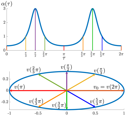
Figure 2: Angular speed $\alpha(\tau,v_{0})$ vs. time $\tau$ for lines moving with the flow (24) for $\omega=1$, $\rho=\frac{1}{3}$, $v_{0}=\begin{pmatrix}1&0\end{pmatrix}^{\top}$ (top). Lines generated by $v(\tau)$ moving on the ellipse $x^{2}+\rho^{-2}y^{2}=1$ (bottom).

4 Application to angular values of linear dynamical systems

In this section we take up the applications which motivated most of the results in previous sections: the theory of angular values for linear nonautonomous dynamical systems. A major step is to extend the definition in [4] from discrete to continuous time systems via the formulas from Section 3.2. Then we investigate for both cases the invariance of angular values under kinematic transformations. This will be the key to the explicit expressions derived in Section 4.3 for the autonomous case with the help of Birkhoff’s ergodic theorem.

4.1 Definition and invariance in the discrete case

From [4, Section 3] we recall several notions of angular values for a nonautonomous linear difference equation

(27) $$u_{n+1}=A_{n}u_{n},\quad A_{n}\in\mathbbm{R}^{d,d},\quad n\in\mathbbm{N}_{0}.$$

We assume that all matrices $A_{n}$ are invertible and that $A_{n}$ as well as $A_{n}^{-1}$ are uniformly bounded. The solution operator is defined by

(28) $$\Phi(n,m)=\begin{cases}A_{n-1}\cdot\ldots\cdot A_{m},&\text{for}\;n>m,\\ I_{d},&\text{for}\;n=m,\\ A_{n}^{-1}\cdot\ldots\cdot A_{m-1}^{-1},&\text{for}\;n<m.\end{cases}$$

Definition 4.1

For $s\in\{1,\ldots,d\}$ and the operator $\Phi$ from (28) define the quantities

(29) $$a_{m,n}(V)=\sum_{j=m}^{n}\measuredangle(\Phi(j-1,0)V,\Phi(j,0)V)\quad m,n\in\mathbbm{N},\;V\in\mathcal{G}(s,d).$$

Then the outer angular values of dimension $s$ are defined by

$$\theta_{s}^{\sup,\varlimsup}=\sup_{V\in\mathcal{G}(s,d)}\varlimsup_{n\to\infty}\frac{1}{n}a_{1,n}(V),\quad\theta_{s}^{\sup,\varliminf}=\sup_{V\in\mathcal{G}(s,d)}\varliminf_{n\to\infty}\frac{1}{n}a_{1,n}(V)$$

and the inner angular values of dimension $s$ are defined by

$$\theta_{s}^{\varlimsup,\sup}=\varlimsup_{n\to\infty}\sup_{V\in\mathcal{G}(s,d)}\frac{1}{n}a_{1,n}(V),\quad\theta_{s}^{\varliminf,\sup}=\varliminf_{n\to\infty}\sup_{V\in\mathcal{G}(s,d)}\frac{1}{n}a_{1,n}(V).$$

Remark 4.2

A common feature of these definitions is that one searches for subspaces $V\in\mathcal{G}(s,d)$ which maximize the longtime average of angles. The attributes ’inner’ and ’outer’ then distinguish cases where the supremum is taken inside or outside the limit as time goes to infinity. At first glance, Definition 4.1 is reminiscent of the well studied notion of rotation numbers for homeomorphisms of the circle; see [8, 16, 20]. Indeed, the notions agree in a very specific two-dimensional case (see [4, Remark 5.3]). However, in general there is a fundamental difference: angular values measure principal angles between subspaces rather than oriented angles between vectors. There is even a difference in two dimensions, since the principal angle of two lines can differ from the oriented angle of two vectors spanning the one-dimensional subspaces. Summarizing, angular values do not contain information about orientation but allow to study the rotation of subspaces of arbitrary dimension in systems of arbitrary dimension. For more comparisons with the literature we refer to [4, Sections 1,5], and a discussion of the continuous time case can be found in Remark 4.6 below.

Note that the following relations hold

(30) $$\begin{matrix}\theta_{s}^{\sup,\varliminf}&\leq&\theta_{s}^{\sup,\varlimsup}\\ \rotatebox[origin={c}]{-90.0}{$\leq$}&&\rotatebox[origin={c}]{-90.0}{$\leq$}\\ \theta_{s}^{\varliminf,\sup}&\leq&\theta_{s}^{\varlimsup,\sup}\end{matrix}$$

and that all inequalities can be strict; see [4, Section 3].

In the following we generalize the invariance of principal angles from Section 2.3 to angular values. We consider a system which is kinematically similar to (27), i.e. we transform variables by $\tilde{u}_{n}=Q_{n}u_{n}$ with $Q_{n}\in\mathrm{GL}(\mathbbm{R}^{d})$ to obtain

(31) $$\tilde{u}_{n+1}=\tilde{A}_{n}\tilde{u}_{n},\quad\tilde{A}_{n}=Q_{n+1}A_{n}Q_{n}^{-1}.$$

The corresponding solution operators $\tilde{\Phi}(n,m)$ and $\Phi(n,m)$ are related by

(32) $$\tilde{\Phi}(n,m)Q_{m}=Q_{n}\Phi(n,m),\quad n\geq m.$$

The following result is more general than [4, Proposition 3.8] and was indicated there without proof.

Proposition 4.3

(Invariance of angular values for discrete systems)

• Let $Q_{n}=q_{n}I_{d}$ with $q_{n}\neq 0$. Then each of the $4$ angular values of the systems (27) and (31) coincide.

• Assume that the transformation matrices satisfy $\lim_{n\to\infty}Q_{n}=Q$, with $Q\in\mathbbm{R}^{d,d}$ being orthogonal. Then the same assertion as in (i) holds.

• Assume that the transformation matrices satisfy $\lim_{n\to\infty}Q_{n}=Q$, with $Q\in\mathbbm{R}^{d,d}$ being invertible. Then an angular value vanishes for the system (27) if and only if the same angular value vanishes for the system (31).

Proof 4.4

(i): From (32) we have $\tilde{\Phi}(n,0)=\frac{q_{n}}{q_{0}}\Phi(n,0)$, hence the spaces $\tilde{\Phi}(n,0)V$ and $\Phi(n,0)V$ agree and the assertion follows from Definition 4.1.

(ii): The main step is to show that for any $\varepsilon>0$ there exists $N=N(\varepsilon)$ such that for all $n\geq N$ and for all $V\in\mathcal{G}(s,d)$

(33) $$S_{n}:=\frac{1}{n}\sum_{j=1}^{n}|\measuredangle(\tilde{\Phi}(j-1,0)Q_{0}V,\tilde{\Phi}(j,0)Q_{0}V)-\measuredangle(\Phi(j-1,0)V,\Phi(j,0)V)|\leq\varepsilon.$$

We use (32), the triangular inequality for $\measuredangle(\cdot,\cdot)$ from Proposition 2.3 and its invariance w.r.t. orthogonal transformations from Section 2.3 to obtain

$$S_{n} =\frac{1}{n}\sum_{j=1}^{n}|\measuredangle(Q_{j-1}\Phi(j-1,0)V,Q_{j}\Phi(j,0)V)-\measuredangle(Q\Phi(j-1,0)V,Q\Phi(j,0)V)|$$

$$\leq\frac{1}{n}\sum_{j=1}^{n}\measuredangle(Q_{j-1}\Phi(j-1,0)V,Q\Phi(j-1,0)V)+\measuredangle(Q_{j}\Phi(j,0)V,Q\Phi(j,0)V)$$

$$=\frac{1}{n}\sum_{j=1}^{n}\measuredangle(Q^{\top}Q_{j-1}\Phi(j-1,0)V,\Phi(j-1,0)V)+\measuredangle(Q^{\top}Q_{j}\Phi(j,0)V,\Phi(j,0)V)$$

$$\leq\frac{C}{n}\sum_{j=1}^{n}\left(\|Q^{\top}Q_{j-1}-I_{d}\|+\|Q^{\top}Q_{j}-I_{d}\|\right),$$

where $C$ is given by Lemma 3.4. Now choose $N_{1}=N_{1}(\varepsilon)$ and then $N=N(\varepsilon)$ such that

$$\|Q^{\top}Q_{j}-I_{d}\|\leq\frac{\varepsilon}{4C}\quad\forall j\geq N_{1},\quad N\geq N_{1}\max(1,\tfrac{\pi}{\varepsilon}).$$

Then we find for $n\geq N$

$$S_{n} =\frac{1}{n}\left[\sum_{j=1}^{N_{1}}\ldots\;+\sum_{j=N_{1}+1}^{n}\ldots\right]\leq\frac{N_{1}}{n}\frac{\pi}{2}+\frac{n-N_{1}}{n}\frac{\varepsilon}{2}\leq\varepsilon.$$

Next consider the outer angular values $\theta_{s}^{\sup,\varlimsup}(A)$ and $\theta_{s}^{\sup,\varlimsup}(\tilde{A})$. Given $\varepsilon>0$ there exists $\tilde{N}(\varepsilon)$ and $V\in\mathcal{G}(s,d)$ such that for all $m\geq\tilde{N}(\varepsilon)$

$$\sup_{n\geq m}\frac{1}{n}\sum_{j=1}^{n}\measuredangle(\Phi(j-1,0)V,\Phi(j,0)V)\geq\theta_{s}^{\sup,\varlimsup}(A)-\frac{\varepsilon}{2}.$$

Using (33) with $\frac{\varepsilon}{2}$ we conclude

$$\sup_{n\geq m}\frac{1}{n}\sum_{j=1}^{n}\measuredangle(\tilde{\Phi}(j-1,0)Q_{0}V,\tilde{\Phi}(j,0)Q_{0}V)\geq\theta_{s}^{\sup,\varlimsup}(A)-\varepsilon.$$

Taking the limit $m\to\infty$ and the supremum over $V\in\mathcal{G}(s,d)$ we obtain the estimate $\theta_{s}^{\sup,\varlimsup}(\tilde{A})\geq\theta_{s}^{\sup,\varlimsup}(A)-\varepsilon$. By symmetry, the same estimate holds when commuting $\tilde{A}$ and $A$. This proves $\theta_{s}^{\sup,\varlimsup}(\tilde{A})=\theta_{s}^{\sup,\varlimsup}(A)$.

The other $3$ angular values are handled in a similar way by employing (33).

(iii): We show that there exists a constant $C_{\star}>0$ and for every $\varepsilon>0$ some $N=N(\varepsilon)$ such that for all $n\geq N$ and for all $V\in\mathcal{G}(s,d)$ the following holds

(34) $$\frac{1}{n}\sum_{j=1}^{n}\measuredangle(\tilde{\Phi}(j-1,0)Q_{0}V,\tilde{\Phi}(j,0)Q_{0}V)\leq\varepsilon+\frac{C_{\star}}{n}\sum_{j=1}^{n}\measuredangle(\Phi(j-1,0)V,\Phi(j,0)V).$$

Since $Q_{n},n\in\mathbbm{N}$ and $Q$ are invertible the condition numbers of $Q_{n}$ are bounded

$$\|Q_{n}\|\|Q_{n}^{-1}\|\leq\kappa,\quad\forall\,n\in\mathbbm{N}.$$

From (32) and the triangle inequality we obtain

$$\frac{1}{n} \sum_{j=1}^{n}\measuredangle(\tilde{\Phi}(j-1,0)Q_{0}V,\tilde{\Phi}(j,0)Q_{0}V)=\frac{1}{n}\sum_{j=1}^{n}\measuredangle(Q_{j-1}\Phi(j-1,0)V,Q_{j}\Phi(j,0)V)$$

$$\leq\frac{1}{n}\sum_{j=1}^{n}\measuredangle(Q_{j-1}\Phi(j-1,0)V,Q_{j-1}\Phi(j,0)V)+\frac{1}{n}\sum_{j=1}^{n}\measuredangle(Q_{j-1}\Phi(j,0)V,Q_{j}\Phi(j,0)V)$$

$$\leq\frac{C_{\star}}{n}\sum_{j=1}^{n}\measuredangle(\Phi(j-1,0)V,\Phi(j,0)V)+\frac{1}{n}\sum_{j=1}^{n}\measuredangle(Q_{j-1}Q_{j}^{-1}Q_{j}\Phi(j,0)V,Q_{j}\Phi(j,0)V)$$

$$\leq\frac{C_{\star}}{n}\sum_{j=1}^{n}\measuredangle(\Phi(j-1,0)V,\Phi(j,0)V)+\frac{C}{n}\sum_{j=1}^{n}\|Q_{j-1}Q_{j}^{-1}-I_{d}\|,$$

with constants $C_{\star}=\pi\kappa(1+\kappa)$ from Lemma 3.1 and $C$ from Lemma 3.4. Let $K$ satisfy $\|Q_{j-1}Q_{j}^{-1}-I_{d}\|\leq K$ for all $j\geq 1$. Now choose $N_{1}=N_{1}(\varepsilon)$ and then $N=N(\varepsilon)$ such that

$$\|Q_{j-1}Q_{j}^{-1}-I_{d}\|\leq\frac{\varepsilon}{2C}\quad\forall j\geq N_{1},\quad N\geq N_{1}\max(1,\tfrac{2CK}{\varepsilon}).$$

Then we find for $n\geq N$

$$\frac{C}{n}\sum_{j=1}^{n}\|Q_{j-1}Q_{j}^{-1}-I_{d}\| =\frac{1}{n}\left[\sum_{j=1}^{N_{1}}\ldots\;+\sum_{j=N_{1}+1}^{n}\ldots\right]\leq\frac{N_{1}}{n}\frac{CK}{2}+\frac{n-N_{1}}{n}\frac{\varepsilon}{2}\leq\varepsilon,$$

which proves (34). Similar to the above, taking the $\varlimsup_{n\to\infty}$ in (34) and then the supremum over $V\in\mathcal{G}(s,d)$ yields

$$\theta_{s}^{\sup,\varlimsup}(\tilde{A})\leq\varepsilon+C_{\star}\theta_{s}^{\sup,\varlimsup}(A).$$

By symmetry, the same estimate holds when commuting $\tilde{A}$ and $A$. This shows that both angular values can only vanish simultaneously. The remaining angular values are analyzed with the help of (34) in a similar way.

4.2 Definition and invariance in the continuous case

In this section we define and investigate angular values for the continuous time system (21). This solves an open problem discussed in [4, Outlook]. Let us first consider a finite interval $[0,T]$ and take Definition 29 in the discrete case as motivation for a proper definition in continuous time. We choose a mesh on $[0,T]$ with stepsize $h=\frac{T}{N}$ and look at the average angle between successive images $V_{jh}=\Phi(jh,0)V$ of $V\in\mathcal{G}(s,d)$ under the time $h$-flow of (21)

$$\theta_{s}(h,T,V) :=\frac{1}{T}\sum_{j=1}^{N}\measuredangle(V_{(j-1)h},V_{jh})$$

$$\phantom{:}=\frac{h}{T}\sum_{j=1}^{N}\frac{1}{h}\left[\measuredangle(V_{(j-1)h},\Phi(jh,(j-1)h)V_{(j-1)h})-\measuredangle(V_{(j-1)h},V_{(j-1)h})\right].$$

From Corollary 3.10 we know that the difference quotients converge as $h\to 0$ and assuming the same for the integral, we obtain

$$\lim_{h\to 0}\theta_{s}(h,T,V) =\frac{1}{T}\int_{0}^{T}\frac{d}{dt}\measuredangle(\Phi(\tau,0)V,\Phi(t,\tau)\Phi(\tau,0)V)_{|t=\tau+}d\tau.$$

Taking the limit $T\to\infty$ and using the formula (22) for the derivative, we end up with the following analog of Definition 4.1.

Definition 4.5

Let the system (21) be given on $[0,\infty)$ and let $\Phi$ be its solution operator. For $V\in\mathcal{G}(s,d)$ with $s\in\{1,\ldots,d\}$ define the quantities

(35) $$a_{t,T}(V)=\int_{t}^{T}\|(I_{d}-P_{\Phi(\tau,0)V})A(\tau)P_{\Phi(\tau,0)V}\|d\tau\quad t,T\in[0,\infty),$$

where $P_{\Phi(\tau,0)V}$ denotes the orthogonal projection onto $\Phi(\tau,0)V$. Then the outer angular values of dimension $s$ are defined by

$$\vartheta_{s}^{\sup,\varlimsup}=\sup_{V\in\mathcal{G}(s,d)}\varlimsup_{T\to\infty}\frac{1}{T}a_{0,T}(V),\quad\vartheta_{s}^{\sup,\varliminf}=\sup_{V\in\mathcal{G}(s,d)}\varliminf_{T\to\infty}\frac{1}{T}a_{0,T}(V),$$

and the inner angular values of dimension $s$ are defined by

$$\vartheta_{s}^{\varlimsup,\sup}=\varlimsup_{T\to\infty}\sup_{V\in\mathcal{G}(s,d)}\frac{1}{T}a_{0,T}(V),\quad\vartheta_{s}^{\varliminf,\sup}=\varliminf_{T\to\infty}\sup_{V\in\mathcal{G}(s,d)}\frac{1}{T}a_{0,T}(V).$$

Remark 4.6

In [1, Ch.6.5] L. Arnold gives a general definition of rotation numbers for vectors in linear continuous time systems. In dimension two his definition amounts to

(36) $$\rho(A)=\lim_{T\to\infty}\frac{1}{T}\int_{0}^{T}\frac{v_{\perp}^{\top}(t)A(t)v(t)}{\|v(t)\|^{2}}dt,\quad v_{\perp}(t)=(-v_{2}(t),v_{1}(t))^{\top},$$

where $v(t)=\Phi(t,0)v_{0}$ solves (21) and the orthogonal vector $v_{\perp}(t)$ is oriented counterclockwise. The integrand in (36) differs just by the absolute value from the expression (23) used for $\vartheta_{s}^{\sup,\varlimsup}$ in Definition 4.1 above. In this sense the maximum rotation number in [1, Ch.6.5] is an oriented version of our angular value for $s=1$. In higher space dimensions the approach in [1, Ch.6.5] differs significantly from angular values with $s=1$. While we use principal angles between one-dimensional subspaces, the generalization in [1, Ch.6.5] utilizes the flow induced by (21) on the Stiefel manifold $\mathrm{St}(2,d)$ and then transfers the two-dimensional rotation number to appropriately moving frames in this manifold.

As in (30) we have the following obvious relations

$$\begin{matrix}\vartheta_{s}^{\sup,\varliminf}&\leq&\vartheta_{s}^{\sup,\varlimsup}\\ \rotatebox[origin={c}]{-90.0}{$\leq$}&&\rotatebox[origin={c}]{-90.0}{$\leq$}\\ \vartheta_{s}^{\varliminf,\sup}&\leq&\vartheta_{s}^{\varlimsup,\sup}\end{matrix}$$

and the elementary estimate $\vartheta_{s}^{\varlimsup,\sup}\leq\sup_{t\geq 0}\|A(t)\|$ if $A(\cdot)$ is uniformly bounded.

Example 4.7

(Example 3.12 revisited)
The angle function $\alpha(\tau,v_{0})$ from (26) is $\frac{\pi}{\omega}$-periodic. Therefore, we obtain from Definition 4.5

$$\vartheta_{1}^{\sup,\varlimsup} =\vartheta_{1}^{\sup,\varliminf}=\sup_{v_{0}\neq 0}\frac{\omega}{\pi}\int_{0}^{\frac{\pi}{\omega}}\alpha(\tau,v_{0})d\tau=\frac{\rho\omega^{2}}{\pi}\sup_{v_{0}\neq 0}\int_{0}^{\frac{\pi}{\omega}}\frac{\|D_{\rho}^{-1}v_{0}\|^{2}}{\|D_{\rho}T_{\tau\omega}D_{\rho}^{-1}v_{0}\|^{2}}d\tau$$

$$=\frac{\rho\omega^{2}}{\pi}\sup_{\|v_{0}\|=1}\int_{0}^{\frac{\pi}{\omega}}\frac{1}{\|D_{\rho}T_{\tau\omega}v_{0}\|^{2}}d\tau=\frac{\rho\omega}{\pi}\sup_{\|v_{0}\|=1}\int_{0}^{\pi}\frac{1}{\|D_{\rho}T_{t}v_{0}\|^{2}}dt.$$

The integrand is $\pi$-periodic, and the integral stays the same if we replace $v_{0}$ by $T_{\varphi}v_{0}$. Therefore, the integral is independent of $v_{0}$ and by taking $v_{0}=\begin{pmatrix}1&0\end{pmatrix}^{\top}$ we obtain

$$\vartheta_{1}^{\sup,\varlimsup} =\vartheta_{1}^{\sup,\varliminf}=\frac{\rho\omega}{\pi}\int_{0}^{\pi}\frac{1}{\cos^{2}(t)+\rho^{2}\sin^{2}(t)}dt=\omega.$$

This result is natural in view of the rotational flow (24) on an ellipse, but it is in stark contrast to the resonance phenomena observed (and proved) for the two-dimensional discrete case in [4, Section 6]. In continuous time we also have $\vartheta_{1}^{\varlimsup,\sup}=\vartheta_{1}^{\varliminf,\sup}=\omega$ for the inner angular values. This can be seen as follows. Write $T=n\frac{2\pi}{\omega}+\tau$ with $n\in\mathbbm{N}_{0}$, $0\leq\tau<\frac{2\pi}{\omega}$ and obtain from the periodicity

$$\frac{1}{T}\int_{0}^{T}\alpha(t,v_{0})dt =\frac{\omega}{2\pi n+\tau\omega}\Big{(}\int_{0}^{n\frac{2\pi}{\omega}}\alpha(t,v_{0})dt+\int_{n\frac{2\pi}{\omega}}^{T}\alpha(t,v_{0})dt\Big{)}$$

$$=\frac{\omega}{2\pi n+\tau\omega}\Big{(}2\pi n+\int_{0}^{\tau}\alpha(t,v_{0})dt\Big{)}.$$

The last integral is uniformly bounded. Hence taking first the supremum with respect to $v_{0}$ and then the limit $n\to\infty$ shows

$$\lim_{T\to\infty}\sup_{v_{0}\neq 0}\int_{0}^{T}\alpha(t,v_{0})dt=\omega.$$

As in Section 4.1 we study the invariance of angular values for (21) on $[0,\infty)$ under a kinematic transformation, i.e. we transform variables by $v(t)=Q(t)u(t)$, $t\geq 0$ where $Q\in C^{1}([0,\infty),\mathrm{GL}(\mathbbm{R}^{d}))$:

(37) $$\dot{v}(t)=\tilde{A}(t)v(t),\quad\tilde{A}(t)=(\dot{Q}(t)+Q(t)A(t))Q(t)^{-1},\quad t\geq 0.$$

Note that the corresponding solution operators $\tilde{\Phi}(t,\tau)$ and $\Phi(t,\tau)$ are related by

(38) $$\tilde{\Phi}(t,\tau)Q(\tau)=Q(t)\Phi(t,\tau),\quad\tau,t\geq 0.$$

Proposition 4.8

(Invariance of angular values for continuous systems) Let the matrices $A\in C([0,\infty),\mathbbm{R}^{d,d})$ be uniformly bounded and let $Q\in C^{1}([0,\infty),\mathrm{GL}(\mathbbm{R}^{d}))$ be given.

• If $Q(t)=q(t)I_{d}$ with $q\in C^{1}([0,\infty),\mathbbm{R})$ then each of the $4$ angular values of the system (21) coincides with the corresponding angular value of the system (37).

• The same assertion as in (i) holds if $\lim_{t\to\infty}\dot{Q}(t)=0$ and if $\lim_{t\to\infty}Q(t)=Q_{\infty}$ exists and is orthogonal.

• If $\lim_{t\to\infty}\dot{Q}(t)=0$ and $Q(\cdot)$, $Q(\cdot)^{-1}$ are uniformly bounded then an angular value of the system (21) vanishes if and only if the corresponding angular value of the system (37) vanishes.

Proof 4.9

(i): In this case we have $\tilde{A}(t)=\frac{\dot{q}(t)}{q(t)}I_{d}+A(t)$ and $\tilde{\Phi}(t,0)=\frac{q(t)}{q(0)}\Phi(t,0)$. Therefore, we have the equality $\Phi(t,0)V=\tilde{\Phi}(t,0)V$ for all $V\in\mathcal{G}(s,d)$ and the expressions $a_{t,T}(V)$ in (35) agree with those of the transformed system. This proves the invariance.

(ii): Similar to (33) we show that for every $\varepsilon>0$ there exists $T_{0}>0$ such that for all $T\geq T_{0}$ and for all $V\in\mathcal{G}(s,d)$:

(39) $$\frac{1}{T}\Big{|}\int_{0}^{T}\|(I_{d}-P_{\tilde{\Phi}(t,0)Q(0)V})\tilde{A}(t)P_{\tilde{\Phi}(t,0)Q(0)V}\|-\|(I_{d}-P_{\Phi(t,0)V})A(t)P_{\Phi(t,0)V}\|dt\Big{|}\leq\varepsilon.$$

To see this, observe that (38) and Proposition 2.3, Lemma 3.4 lead to

(40) $$\|P_{\tilde{\Phi}(t,0)Q(0)V}-Q_{\infty}P_{\Phi(t,0)V}Q_{\infty}^{\top}\|=\|P_{Q(t)\Phi(t,0)V}-P_{Q_{\infty}\Phi(t,0)V}\|$$

$$\leq\measuredangle(Q(t)\Phi(t,0)V,Q_{\infty}\Phi(t,0)V)=\measuredangle(Q_{\infty}^{\top}Q(t)\Phi(t,0)V,\Phi(t,0)V)$$

$$\leq C\|Q_{\infty}Q(t)-I_{d}\|=C\|Q(t)-Q_{\infty}\|\to 0\quad\text{as}\;t\to\infty.$$

With (37) and the orthogonality of $Q_{\infty}$ we estimate the lefthand side of (39) by

$$\frac{1}{T}\int_{0}^{T}\Big{|}\|(I_{d}-P_{\tilde{\Phi}(t,0)Q(0)V})\tilde{A}(t)P_{\tilde{\Phi}(t,0)Q(0)V}\|-\|Q_{\infty}(I_{d}-P_{\Phi(t,0)V})A(t)P_{\Phi(t,0)V}Q_{\infty}^{\top}\|\Big{|}dt$$

$$\leq\frac{1}{T}\Big{[}\int_{0}^{T}\|(I_{d}-P_{\tilde{\Phi}(t,0)Q(0)V})\dot{Q}(t)Q^{-1}(t)P_{\tilde{\Phi}(t,0)Q(0)V}\|$$

$$\qquad\qquad+\|(I_{d}-P_{\tilde{\Phi}(t,0)Q(0)V})Q(t)A(t)Q(t)^{-1}P_{\tilde{\Phi}(t,0)Q(0)V}$$

$$\qquad\qquad-Q_{\infty}(I_{d}-P_{\Phi(t,0)V})Q_{\infty}^{\top}Q_{\infty}A(t)Q_{\infty}^{\top}Q_{\infty}P_{\Phi(t,0)V}Q_{\infty}^{\top}\|dt\Big{]}.$$

From the convergence of projectors in (40) and from $Q(t)\to Q_{\infty}$, $Q(t)^{-1}\to Q_{\infty}^{\top}$, $\dot{Q}(t)\to 0$ as $t\to\infty$ we conclude via the boundedness of $A(t)$ that the integrand converges to zero as $t\to\infty$ uniformly in $V\in\mathcal{G}(s,d)$. Thus (39) can be achieved by taking $T$ sufficiently large.

Consider now the outer angular values $\vartheta_{s}^{\sup,\varlimsup}(A)$ and $\vartheta_{s}^{\sup,\varlimsup}(\tilde{A})$. Given $\varepsilon>0$ there exists $V\in\mathcal{G}(s,d)$ and $T_{0}=T_{0}(\varepsilon,V)$ such that

$$\sup_{T\geq T_{0}}\frac{1}{T}\int_{0}^{T}\|(I_{d}-P_{\Phi(t,0)V}A(t)P_{\Phi(t,0)V}\|dt\geq\vartheta_{s}^{\sup,\varlimsup}(A)-\frac{\varepsilon}{2}.$$

Using (39) with $\frac{\varepsilon}{2}$ we conclude for $T_{0}$ sufficiently large

$$\sup_{T\geq T_{0}}\frac{1}{T}\int_{0}^{T}(I_{d}-P_{\tilde{\Phi}(t,0)Q(0)V})\tilde{A}(t)P_{\tilde{\Phi}(t,0)V}\|dt\geq\vartheta_{s}^{\sup,\varlimsup}(A)-\varepsilon.$$

Taking the limit $T_{0}\to\infty$ and the supremum over $V\in\mathcal{G}(s,d)$ we obtain the estimate $\vartheta_{s}^{\sup,\varlimsup}(\tilde{A})\geq\vartheta_{s}^{\sup,\varlimsup}(A)-\varepsilon$. By symmetry, the same estimate holds when commuting $\tilde{A}$ and $A$. This proves $\vartheta_{s}^{\sup,\varlimsup}(\tilde{A})=\vartheta_{s}^{\sup,\varlimsup}(A)$. The other $3$ angular values are handled in a similar way by employing (39).

(iii): For this proof it suffices to show that there exists a constant $C_{\star}$ and for every $\varepsilon>0$ some $T_{0}$ such that for all $T\geq T_{0}$ and $V\in\mathcal{G}(s,d)$ the following holds

(41) $$\frac{1}{T}\int_{0}^{T}\|(I_{d}-P_{\tilde{\Phi}(t,0)Q(0)V})\tilde{A}(t)P_{\tilde{\Phi}(t,0)Q(0)V}\|dt\leq\varepsilon+\frac{C_{\star}}{T}\int_{0}^{T}\|(I_{d}-P_{\Phi(t,0)V})A(t)P_{\Phi(t,0)V}\|dt.$$

Instead of (40) we use the following identities

$$(I_{d}-P_{Q(t)\Phi(t,0)V})Q(t) =(I_{d}-P_{Q(t)\Phi(t,0)V})Q(t)(I_{d}-P_{\Phi(t,0)V}),$$

$$Q(t)^{-1}P_{Q(t)\Phi(t,0)V} =P_{\Phi(t,0)V}Q(t)^{-1}P_{Q(t)\Phi(t,0)V}.$$

These lead to the following estimate

$$\|(I_{d}-P_{\tilde{\Phi}(t,0)Q(0)V})\tilde{A}(t)P_{\tilde{\Phi}(t,0)Q(0)V}\|=\|(I_{d}-P_{Q(t)\Phi(t,0)V})\tilde{A}(t)P_{Q(t)\Phi(t,0)V}\|$$

$$\leq\|(I_{d}-P_{Q(t)\Phi(t,0)V})\dot{Q}(t)Q(t)^{-1}P_{Q(t)\Phi(t,0)V}\|$$

$$\phantom{=\ }+\|(I_{d}-P_{Q(t)\Phi(t,0)V})Q(t)(I_{d}-P_{\Phi(t,0)V})A(t)P_{\Phi(t,0)V}Q(t)^{-1}P_{Q(t)\Phi(t,0)V}\|$$

$$\leq\|Q^{-1}\|_{\infty}\|\dot{Q}(t)\|+\|Q\|_{\infty}\|Q^{-1}\|_{\infty}\|(I_{d}-P_{\Phi(t,0)V})A(t)P_{\Phi(t,0)V}\|.$$

Our assumptions on $Q$ then guarantee that (41) holds for $T$ sufficiently large with the constant $C_{\star}=\|Q\|_{\infty}\|Q^{-1}\|_{\infty}$. Suppose that $\vartheta_{s}^{\sup,\varlimsup}(A)=0$. Then for all $V\in\mathcal{G}(s,d)$ and for each $\varepsilon>0$ there exists $T_{0}=T_{0}(\varepsilon,V)$ such that

$$\sup_{T\geq T_{0}}\frac{1}{T}\int_{0}^{T}\|(I_{d}-P_{\Phi(t,0)V})A(t)P_{\Phi(t,0)V}\|dt\leq\varepsilon.$$

Combining this with (41) we obtain

$$\sup_{T\geq T_{0}}\frac{1}{T}\int_{0}^{T}\|(I_{d}-P_{\tilde{\Phi}(t,0)Q(0)V})\tilde{A}(t)P_{\tilde{\Phi}(t,0)Q(0)V}\|dt\leq(1+C_{\star})\varepsilon$$

for $T_{0}$ sufficiently large. Therefore, the limit as $T_{0}\to\infty$ vanishes and recalling that this holds for all $V$, we end up with $\vartheta_{s}^{\sup,\varlimsup}(\tilde{A})=0$. The other angular values are treated by using (41) in a similar manner.

Remark 4.10

If we replace $A(t)$ in (21) by $A(t)+\lambda(t)I_{d}$, then angular values remain unchanged. This follows from case (i) by setting $q(t)=\exp\big{(}\int_{0}^{t}\lambda(\tau)d\tau\big{)}$. In particular, we can choose $\lambda(t)=-\frac{1}{d}\mathrm{tr}(A(t))$. Hence the computation of angular values can be restricted to systems (21) satisfying $\mathrm{tr}(A(t))=0$ for $t\in[0,\infty)$.

4.3 Some formulas for autonomous systems

In the following we apply the results of the previous section to the autonomous system

(42) $$\dot{u}=Au,\quad A\in\mathbbm{R}^{d,d}.$$

Proposition 4.8 (ii) suggests to look at the real quasitriangular Schur form of $A$:

(43) $$QAQ^{\top} =\begin{pmatrix}\Lambda_{11}&\Lambda_{12}&\cdots&\Lambda_{1k}\\ 0&\Lambda_{22}&\cdots&\Lambda_{2k}\\ \vdots&\ddots&\ddots&\vdots\\ 0&\cdots&0&\Lambda_{kk}\end{pmatrix},\quad Q^{\top}Q=I_{d},\quad\Lambda_{ij}\in\mathbbm{R}^{d_{i},d_{j}},$$

$$\Lambda_{jj} =\begin{cases}\begin{pmatrix}\beta_{j}&-\frac{\omega_{j}}{\rho_{j}}\\ \rho_{j}\omega_{j}&\beta_{j}\end{pmatrix}\in\mathbbm{R}^{2,2},&d_{j}=2,\omega_{j}>0,\quad 0<\rho_{j}\leq 1,\\ \lambda_{j}=\beta_{j}\in\mathbbm{R},&d_{j}=1,\end{cases}$$

$$\beta_{1}\geq\cdots\geq\beta_{k}.$$

We refer to [14, Theorem 2.3.4] and emphasize the special form of the blocks $\Lambda_{jj}$ with nonreal eigenvalues $\lambda_{j}=\beta_{j}+i\omega_{j}$; cf. Example 3.12. Further, we introduce

$$J_{\mathbbm{C}}=\{j\in\{1,\ldots,k\}:d_{j}=2\}.$$

As a preparation we determine the asymptotic behavior of the orthogonal projections $P_{e^{tA}V}$ for a given element $V=\mathcal{R}(W)\in\mathcal{G}(s,d)$ with $W\in\mathbbm{R}^{d,s}$. By column operations we can put $W$ into block column echelon form. Within the blocks, the number of rows is given by the sequence $d_{1},\ldots,d_{k}$ from (43) while the number of columns is either $1$ or $2$:

(44) $$W =\begin{pmatrix}0&0&\cdots&0\\ W_{k_{1}+1,1}&0&\cdots&0\\ \vdots&W_{k_{2}+1,2}&&\vdots\\ \vdots&\vdots&\ddots&W_{k_{r}+1,r}\\ \vdots&\vdots&\vdots&\vdots\\ W_{k,1}&W_{k,2}&\cdots&W_{k,r}\end{pmatrix},\quad\big{(}W_{ij}\in\mathbbm{R}^{d_{i},b_{j}}\big{)}_{i=1,\ldots,k}^{j=1,\ldots,r},$$

$$s =\sum_{j=1}^{r}b_{j},\quad\text{where}\quad b_{j}\begin{cases}=1,&\text{if}\,d_{k_{j}+1}=1,\\ \in\{1,2\},&\text{if}\,d_{k_{j}+1}=2.\end{cases}$$

Here the indices $0\leq k_{1}<k_{2}<\cdots<k_{r}<k$ are determined such that

$$W_{ij}=0\;(i=1,\ldots,k_{j}),\quad{\rm{rank}}(W_{k_{j}+1,j})=b_{j},\quad j=1,\ldots,r.$$

Note that the leading entry $W_{k_{j}+1,j}$ is of size $2\times 1$ or $2\times 2$ if $k_{j}+1\in J_{\mathbbm{C}}$ and of size $1\times 1$ otherwise. Further, the numbers $k_{j}$ and the ranges $\mathcal{R}(W_{k_{j}+1,j})$, $j=1,\ldots,r$ are unique.

Example 4.11

Consider a continuous system (42) in $\mathbbm{R}^{4}$ with matrices

(45) $$A=A(\omega,\rho)=\begin{pmatrix}\Lambda_{11}&0\\ 0&\Lambda_{22}\end{pmatrix},\quad\Lambda_{jj}=\begin{pmatrix}j-1&-\frac{\omega_{j}}{\rho_{j}}\\ \rho_{j}\omega_{j}&j-1\end{pmatrix},\quad j=1,2,$$

where $\omega=(\omega_{1},\omega_{2})\in(0,\infty)^{2}$, $\rho=(\rho_{1},\rho_{2})\in(0,1]^{2}$. We have $d=4$, $k=2$, $J_{\mathbbm{C}}=\{1,2\}$ and we chose different diagonal elements in $\Lambda_{jj}$, $j=1,2$ so that Lemma 4.12 below applies. Then the following choices for the column echelon form (44) are possible:

(46) $$s=1: \quad(k_{1}=0,b_{1}=1)\;\text{or}\;(k_{1}=1,b_{1}=1),$$

$$s=2: \quad(k_{1}=0,b_{1}=1,k_{2}=1,b_{2}=1)\;\text{or}\;(k_{1}=0,b_{1}=2)\;\text{or}\;(k_{1}=1,b_{1}=2),$$

$$s=3: \quad(k_{1}=0,b_{1}=1,k_{2}=1,b_{2}=2)\;\text{or}\;(k_{1}=0,b_{1}=2,k_{2}=1,b_{2}=1).$$

As we will see below, the cases where at least one $b_{j}=1$ occurs, are most relevant for the angular value.

To take care of multiple real eigenvalues we determine numbers $\ell_{j}\in\{1,\ldots,k-1\}$ for $j=1,\ldots,r$ with

(47) $$\beta_{k_{j}+1}=\cdots=\beta_{k_{j}+\ell_{j}}>\beta_{k_{j}+\ell_{j}+1}.$$

Further, we assume isolated real parts of the eigenvalues $\lambda_{j}=\beta_{j}+i\omega_{j}$, $j\in J_{\mathbbm{C}}$, i.e.

(48) $$\beta_{j}\neq\beta_{\nu}\quad\forall j\in J_{\mathbbm{C}},\ \nu\in\{1,\ldots,k\},\ \nu\neq j,$$

which implies $\ell_{j}=1$ if $k_{j}+1\in J_{\mathbbm{C}}$. With these data we define $W^{\infty}\in\mathbbm{R}^{d,s}$ and its image space $V^{\infty}=\mathcal{R}(W^{\infty})$ by

(49) $$W^{\infty}_{i,j} =\begin{cases}W_{i,j},&k_{j}+1\leq i\leq k_{j}+\ell_{j},\quad j\in\{1,\ldots,r\},\\ 0,&\text{otherwise}.\end{cases}$$

Complex eigenvalues lead to single blocks in $W^{\infty}$ while a sequence of $\ell_{j}$ identical real eigenvalues leads to a full rank lower triangular block matrix with at most $\ell_{j}$ columns.

Lemma 4.12

Let condition (48) hold. Then the spaces $V,V^{\infty}$ defined above satisfy

$$P_{e^{tA}V}-P_{e^{tA}V^{\infty}}\to 0\quad\text{as}\quad t\to\infty.$$

Proof 4.13

Define $B=\mathrm{diag}\big{(}(\beta_{k_{j}+1}I_{b_{j}})_{j=1}^{r}\big{)}\in\mathbbm{R}^{s,s}$ and observe that the matrices $U(t)=e^{tA}We^{-tB}$ and $U^{\infty}(t)=e^{tA}W^{\infty}e^{-tB}$ satisfy

$$\big{(}U(t)-U^{\infty}(t)\big{)}_{i,j}=\begin{cases}(e^{t\Lambda_{ii}}e^{-t\beta_{k_{j}+1}})W_{ij},&i>k_{j}+\ell_{j},\\ 0,&\text{otherwise}.\end{cases}$$

By (48) and the ordering in (47) we obtain for some constants $C,\gamma>0$

$$\|U(t)-U^{\infty}(t)\|\leq Ce^{-\gamma t},\quad t\geq 0.$$

The leading entries of $U^{\infty}(t)$ are

$$U^{\infty}_{k_{j}+1,j}(t)=\begin{cases}W_{k_{j}+1,j},&\text{if}\,d_{k_{j}+1}=1,\\ D_{\rho_{k_{j}+1}}T_{t\omega_{k_{j}+1}}D_{\rho_{k_{j}+1}}^{-1}W_{k_{j}+1,j},&\text{if}\,d_{k_{j}+1}=2,\end{cases}$$

where $D_{\rho},T_{\omega}$ are defined in (25). The matrices $(U^{\infty}(t)^{\top}U^{\infty}(t))^{-1}\in\mathbbm{R}^{s,s}$ are uniformly bounded since the entries $W_{k_{j}+1,j}$ have maximum rank and the rotations $T_{t\omega}$ are uniformly bounded. Further, the matrix $S(t)=U(t)(U^{\infty}(t)^{\top}U^{\infty}(t))^{-1}U^{\infty}(t)^{\top}\in\mathbbm{R}^{d,d}$ satisfies

$$S(t)U^{\infty}(t)=U(t),\quad S(t)e^{tA}W^{\infty}=e^{tA}W,\quad t\geq 0.$$

For every $v=U^{\infty}(t)e^{tB}b=e^{tA}W^{\infty}b\in e^{tA}V^{\infty}$, $b\in\mathbbm{R}^{s}$ we have the estimate

$$\|(S(t)-I_{d})v\| =\|S(t)e^{tA}W^{\infty}b-e^{tA}W^{\infty}b\|=\|e^{tA}Wb-e^{tA}W^{\infty}b\|$$

$$=\|(U(t)-U^{\infty}(t))e^{tB}b\|\leq Ce^{-\gamma t}\|e^{tB}b\|$$

$$=Ce^{-\gamma t}\|(U^{\infty}(t)^{\top}U^{\infty}(t))^{-1}U^{\infty}(t)^{\top}v\|\leq Ce^{-\gamma t}\|v\|.$$

For $t$ sufficiently large this leads to

$$\|(I_{d}-S(t))v\| \leq\frac{Ce^{-\gamma t}}{1-Ce^{-\gamma t}}\|S(t)v\|\quad\forall v\in e^{tA}V^{\infty}.$$

Thus we can apply Lemma 3.2 (ii) and use (4) to obtain our assertion

$$\|P_{e^{tA}V^{\infty}}-P_{e^{tA}V}\| \leq\measuredangle(e^{tA}V^{\infty},e^{tA}V)=\measuredangle(e^{tA}V^{\infty},S(t)e^{tA}V^{\infty})\leq Ce^{-\gamma t}.$$

The following proposition provides the angular value in two cases where the asymptotics of $P_{e^{tA}V^{\infty}}$ is easy to analyze.

Proposition 4.14

Assume that the real Schur form (43) of $A$ is blockdiagonal with isolated real parts of complex eigenvalues as in (48). Then the following assertions hold:

• If all eigenvalues are real then

  (50) $$\vartheta_{s}^{\sup,\varlimsup}(A)=\vartheta_{s}^{\sup,\varliminf}(A)=0.$$

• If $J_{\mathbbm{C}}$ is nonempty and $s\in\{1,d-1\}$ or ($|J_{\mathbbm{C}}|=1$, $s<d$) then

  (51) $$\vartheta_{s}^{\sup,\varlimsup}(A)=\vartheta_{s}^{\sup,\varliminf}(A)=\max_{j\in J_{\mathbbm{C}}}\omega_{j}.$$

Remark 4.15

Clearly, equation (50) may be regarded as a special case of (51) by setting $\max_{\emptyset}=0$.

Proof 4.16

By Proposition 4.8 (iii) we can assume $A$ to be in Schur normal form (43).

• In this case we have $A=\mathrm{diag}(\lambda_{1},\ldots,\lambda_{d})$ with $\lambda_{1}\geq\lambda_{2}\geq\cdots\geq\lambda_{d}$. Then the space $V^{\infty}=\mathcal{R}(W^{\infty})$ defined by (49) is spanned by Cartesian basis vectors, hence $A$ and $e^{tA}$ leave $V^{\infty}$ invariant and

  $$(I_{d}-P_{e^{tA}V^{\infty}})AP_{e^{tA}V^{\infty}}=(I_{d}-P_{V^{\infty}})AP_{V^{\infty}}=0\quad\forall\ t\geq 0.$$

  Lemma 4.12 shows $(I_{d}-P_{e^{tA}V})AP_{e^{tA}V}\to 0$ and the assertion follows from Definition 4.5.

• Consider first $s=1$. If $k_{1}+1\notin J_{\mathbbm{C}}$ then $V^{\infty}$ is invariant under $A$. Hence we have $(I_{d}-P_{e^{tA}V^{\infty}})AP_{e^{tA}V^{\infty}}=0$ and $\lim_{T\to\infty}\frac{1}{T}a_{0,T}(V)=0$ as above. If $k_{1}+1\in J_{\mathbbm{C}}$ then we find from Example 4.7

  $$\lim_{T\to\infty}\frac{1}{T}a_{0,T}(V^{\infty}) =\frac{\rho_{k_{1}+1}\omega_{k_{1}+1}}{\pi}\int_{0}^{\pi}\frac{\|W_{k_{1}+1,1}\|^{2}}{\|D_{\rho_{k_{1}+1}}T_{t}W_{k_{1}+1,1}\|^{2}}dt=\omega_{k_{1}+1}.$$

  Taking the maximum over $V\in\mathcal{G}(1,d)$ then proves (51).

  In case $1\leq s<d$ and $|J_{\mathbbm{C}}|=1$ there are three possibilities. If $k_{j}+1\notin J_{\mathbbm{C}}$ for all $j=1,\ldots,r$ then $V^{\infty}$ is invariant under $A$ and $\lim_{T\to\infty}\frac{1}{T}a_{0,T}(V)=0$ as above. Otherwise, there exists exactly one $j\in\{1,\ldots,r\}$ with $k_{j}+1\in J_{\mathbbm{C}}$. If $b_{j}=2$ then $W_{k_{j}+1,j}\in\mathbbm{R}^{2,2}$ is invertible and

  $$\Lambda_{k_{j}+1,k_{j}+1}W_{k_{j}+1,j}=W_{k_{j}+1,j}M_{j},\quad\text{for}\;M_{j}=W_{k_{j}+1,j}^{-1}\Lambda_{k_{j}+1,k_{j}+1}W_{k_{j}+1,j}.$$

  Hence $V^{\infty}$ is invariant, again leading to the limit zero. The final case is $b_{j}=1$ which occurs at least once since $s<d$. Then the only nonzero block row of $(I_{d}-P_{e^{tA}V^{\infty}})AP_{e^{tA}V^{\infty}}$ is given by

  (52) $$\big{(}I_{2}-P_{V_{j}(t)}\big{)}\Lambda_{k_{j}+1,k_{j}+1}P_{V_{j}(t)},\quad\text{where}\;V_{j}(t)=\mathrm{span}(e^{t\Lambda_{k_{j}+1,k_{j}+1}}W_{k_{j}+1,j}).$$

  The spectral norm of this $2\times 2$ matrix yields the spectral norm of $(I_{d}-P_{e^{tA}V^{\infty}})AP_{e^{tA}V^{\infty}}$ and leads to $\lim_{T\to\infty}\frac{1}{T}a_{0,T}(V^{\infty})=\omega_{k_{j}+1}$ as above. This proves (51).

  Finally, let $s=d-1$. Since $\sum_{j=1}^{r}b_{j}=s$ for the column echelon form (44) there is exactly one index $j\in\{1,\ldots,r\}$ with $b_{j}=1$, $d_{k_{j}+1}=2$ while all $b_{\nu}$, $\nu\neq j$ attain their maximum value (either $1$ or $2$). As above, the only nonzero block row of $(I_{d}-P_{e^{tA}V^{\infty}})AP_{e^{tA}V^{\infty}}$ is given by (52) and we obtain $\lim_{T\to\infty}\frac{1}{T}a_{0,T}(V^{\infty})=\omega_{k_{j}+1}$ and then formula (51) by maximizing over $V\in\mathcal{G}(d-1,d)$.

Next we consider the case of general dimension $s$ and arbitrary index set $J_{\mathbbm{C}}$. As we have seen above, only the leading entries $W_{k_{j}+1,j}$ with $b_{j}=1$ contribute to the angular value. Therefore, we determine those index sets $J\subseteq J_{\mathbbm{C}}$ which belong to elements $V\in\mathcal{G}(s,d)$ with $b_{j}=1$ for $j\in J$. We call these sets admissible and show that they are given by

(53) $$\mathcal{J}(s,\mathbbm{C})=\{J\subseteq J_{\mathbbm{C}}:|J|\leq\min(s,d-s)\quad\text{and}\quad(s-|J|\;\text{is even, if}\;|J_{\mathbbm{C}}|=k)\}.$$

Lemma 4.17

A subset $J\subseteq J_{\mathbbm{C}}$ belongs to $\mathcal{J}(s,\mathbbm{C})$ if and only if there exists $V\in\mathcal{G}(s,d)$ with $V=\mathcal{R}(W)$ such that the column echelon form (44) of $W$ has $b_{j}=1$, $d_{k_{j}+1}=2$ exactly for the indices $j\in J$.

Proof 4.18

First assume that an appropriate $V\in\mathcal{G}(s,d)$ exists. Then the estimate $|J|\leq s$ follows from (44), since the columns which belong to $j\in J$ are linearly independent. By dimension counting we further have $s=|J|+n_{1}+2n_{2}$ where $0\leq n_{1}\leq k-|J_{\mathbbm{C}}|$ (number of real eigenvalues) and $0\leq n_{2}\leq|J_{\mathbbm{C}}|-|J|$ (number of remaining complex eigenvalues). If $k=|J_{\mathbbm{C}}|$ then $n_{1}=0$ and $s-|J|\geq 0$ is even. In general, we have

(54) $$s\leq|J|+k-|J_{\mathbbm{C}}|+2(|J_{\mathbbm{C}}|-|J|)=k+|J_{\mathbbm{C}}|-|J|=d-|J|,$$

whence $|J|\leq d-s$. Conversely, assume $J\in\mathcal{J}(s,\mathbbm{C})$ so that the inequality (54) holds. If $k=|J_{\mathbbm{C}}|$ then $s-|J|$ is even and we have $s=|J|+2n_{2}$, where $0\leq n_{2}\leq|J_{\mathbbm{C}}|-|J|$ follows from (54). If $k-|J_{\mathbbm{C}}|\geq 1$ holds, we set $n_{2}=\min(\lfloor\frac{s-|J|}{2}\rfloor,|J_{\mathbbm{C}}|-|J|)\geq 0$ and $n_{1}=s-|J|-2n_{2}$. Then we have $n_{1}\geq s-|J|-2\lfloor\frac{s-|J|}{2}\rfloor\geq 0$. Further, if $n_{2}=\lfloor\frac{s-|J|}{2}\rfloor$ we conclude $n_{1}\in\{0,1\}$, hence $n_{1}\leq k-|J_{\mathbbm{C}}|$. In case $n_{2}=|J_{\mathbbm{C}}|-|J|$ we find from (54)

$$n_{1} \leq k-|J_{\mathbbm{C}}|+2(|J_{\mathbbm{C}}|-|J|)-2n_{2}=k-|J_{\mathbbm{C}}|,$$

as required. Summarizing, we can construct some $V=\mathcal{R}(W)\in\mathcal{G}(s,d)$ with a matrix $W$ of rank $s$ as in (44) with $|J|$ columns belonging to indices in $J_{\mathbbm{C}}$, $n_{2}$ double columns belonging to the remaining complex eigenvalues, and $n_{1}$ columns belonging to real eigenvalues.

Proposition 4.19

Assume that the real Schur form (43) of $A$ is blockdiagonal with nonempty $J_{\mathbbm{C}}$ and isolated real parts as in (48). Then the following holds:

• For $1\leq s\leq d-1$, $\vartheta_{s}^{\sup,\varlimsup}(A)=\vartheta_{d-s}^{\sup,\varlimsup}(A)$, $\vartheta_{s}^{\sup,\varliminf}(A)=\vartheta_{d-s}^{\sup,\varliminf}(A)$.

• If the values $\omega_{j}$, $j\in J$ are rationally independent for every $J\in\mathcal{J}(s,\mathbbm{C})$, then the outer angular values are given by

  (55) $$\vartheta_{s}^{\sup,\varlimsup}(A) =\vartheta_{s}^{\sup,\varliminf}(A)=\max_{J\in\mathcal{J}(s,\mathbbm{C})}\frac{1}{\pi^{|J|}}\int_{[0,\pi]^{|J|}}\max_{j\in J}E_{j}(\tau_{j})\,d(\tau_{j})_{j\in J},$$

  $$E_{j}(\tau_{j}) =\frac{\rho_{j}\omega_{j}}{\cos^{2}(\tau_{j})+\rho_{j}^{2}\sin^{2}(\tau_{j})}.$$

Remarks 4.20

• Recall from [16, Prop.1.4.1] that numbers $a_{1},\ldots,a_{r}\in\mathbbm{R}$ are rationally independent if $\sum_{j=1}^{r}m_{j}a_{j}=0$ for some $m_{j}\in\mathbbm{Z}$ implies $m_{1}=\cdots=m_{r}=0$. In particular, in the simple case $s=1$ or $|J_{\mathbbm{C}}|=1$ each single value $\omega_{j}\neq 0$ is rationally independent so that (51) becomes a special case of the formula (55). In case $s=d$ we have $\vartheta_{s}^{\sup,\lim}(A)=0$ which is consistent with (55) when setting $\max_{\emptyset}=0$.

• Estimating $\max_{j\in J}E_{j}\geq E_{\ell}$ for each $\ell\in J$ in (55) leads to the lower bound $\vartheta_{s}^{\sup,\lim}(A)\geq\max_{j\in J_{\mathbbm{C}}}\omega_{j}$, since for every $j\in J_{\mathbbm{C}}$ there is an element $J\in\mathcal{J}(s,\mathbbm{C})$ with $j\in J$. Similarly, the integral expression in (55) grows when passing from $J^{\prime}\in\mathcal{J}(s,\mathbbm{C})$ to some $J\in\mathcal{J}(s,\mathbbm{C})$ with $J^{\prime}\subset J$. Therefore, it suffices to consider only maximal index sets $J\in\mathcal{J}(s,\mathbbm{C})$ in (55).

• Recall that normal matrices have a block diagonal real Schur form [14, Theorem 2.5.8]. However, $\Lambda_{jj}$ in (43) is not normal if $\rho_{j}<1$. Hence, Propositions 4.14, 4.19 cover a class of nonnormal matrices.

• Let us finally mention that Propositions 4.14, 4.19 can be extended in several ways. First, the inner angular values $\vartheta_{s}^{\varlimsup,\sup}(A)$, $\vartheta_{s}^{\varliminf,\sup}(A)$ agree with the outer ones in both assertions. Second, one can treat normal forms with nonzero blocks above the diagonal in (43). A proof of these results needs reduction techniques analogous to those of the discrete case; see [4, Section 5], [5, Section 3]. Moreover, relaxing the assumption on rational independence requires further tools, such as unique ergodicity and the ergodic decomposition theorem ([16, Ch.4.1,4.2], [2, Theorem 3.3]). The corresponding results and their proofs are beyond the scope of this paper.

Example 4.21

(Example 4.11 revisited)
From (46) we infer that the admissible index sets are given by

$$\mathcal{J}(1,\mathbbm{C})=\{\{1\},\{2\}\},\quad\mathcal{J}(2,\mathbbm{C})=\{\{1,2\}\},\quad\mathcal{J}(3,\mathbbm{C})=\{\{1\},\{2\}\}.$$

By Proposition 4.14 (ii) we have $\vartheta_{1}^{\sup,\lim}(A)=\max(\omega_{1},\omega_{2})=\vartheta_{3}^{\sup,\lim}(A)$. At first glance, this equality may come as a surprise, but Proposition 4.19 (i) shows that this symmetry holds in general. For this example, subspaces of dimension $s=2$ are the most interesting ones since they have more flexibility to rotate. Figure 3 shows the graph of the integrand in (55) for the case $s=2=|J_{\mathbbm{C}}|$ with the rationally independent values $\omega_{1}=1$, $\omega_{2}=\frac{1}{\sqrt{2}}$. Numerical integration yields the angular value $\vartheta_{2}^{\sup,\lim}(A)=1.2693394>\max(\omega_{1},\omega_{2})=1$.

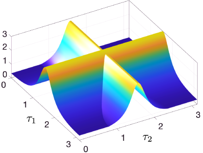
Figure 3: Graph of the integrand from (55) for the two-dimensional case $J=\{1,2\}$. Parameter values: $\rho_{1}=\frac{1}{3}$, $\omega_{1}=1$, $\rho_{2}=\frac{1}{4}$, $\omega_{2}=\frac{1}{\sqrt{2}}$.

Proof 4.22

By Proposition 4.8 (ii) we can assume $A$ itself to be in Schur normal form (43) and by Lemma 4.12 it suffices to compute the angular value for $V^{\infty}=\mathcal{R}(W^{\infty})$ from (49). The projections $P_{e^{tA}V^{\infty}}$ are direct products of projections which either belong to a simple complex eigenvalue or to a group of identical real eigenvalues. As we have seen above, the latter ones and the projections onto $(0\cdots 0\ W_{k_{j}+1,j}\ 0\cdots 0)^{\top}$ with $d_{k_{j}+1}=2$, $b_{j}=2$ lead to zero terms in $(I_{d}-P_{e^{tA}V^{\infty}})AP_{e^{tA}V^{\infty}}$. Hence, the spectral norm is determined by index sets $J\in\mathcal{J}(s,\mathbbm{C})$ and their corresponding elements in $\mathcal{G}(s,d)$ from Lemma 4.17. More specifically, the spectral norm is computed from the vectors $W_{k_{j}+1,j}\in\mathbbm{R}^{2}$, $j\in J$ and the spaces $V_{j}(t)$, $j\in J$ in (52) as follows:

(56) $$\|(I_{d}-P_{e^{tA}V^{\infty}})AP_{e^{tA}V^{\infty}})\| =\max_{j\in J}\|(I_{2}-P_{V_{j}(t)})\Lambda_{k_{j}+1,k_{j}+1}P_{V_{j}(t)}\|.$$

• This assertion follows from (56) and the equality $\mathcal{J}(s,\mathbbm{C})=\mathcal{J}(d-s,\mathbbm{C})$ for the sets in (53). To see this, note that the condition $|J|\leq\min(s,d-s)$ is symmetric. Further, if $k=|J_{\mathbbm{C}}|$ holds then $d=2k$ is even, hence $s-|J|$ and $d-s-|J|$ have the same parity.

• In the following we write the function $\alpha$ from (26) as

  (57) $$\alpha(\tau,v,\rho,\omega)=\frac{\rho\omega\|D_{\rho}^{-1}v\|^{2}}{\|D_{\rho}T_{\tau\omega}D_{\rho}^{-1}v\|^{2}},\quad\tau\in\mathbbm{R},v\in\mathbbm{R}^{2}\setminus\{0\},\ 0<\rho\leq 1,\ \omega>0.$$

  The function has the following properties

  (58) $$\alpha(\tau+\tfrac{2\pi}{\omega},v,\rho,\omega) =\alpha(\tau,v,\rho,\omega),$$

  $$\alpha(\tau,xv,\rho,\omega) =\alpha(\tau,v,\rho,\omega),\quad x\in\mathbbm{R},$$

  $$\alpha(\tau,D_{\rho}T_{t\omega}D_{\rho}^{-1}v,\rho,\omega) =\alpha(\tau+t,v,\rho,\omega),\quad t\in\mathbbm{R}.$$

  For $J\subseteq J_{\mathbbm{C}}$ we introduce the $|J|$-dimensional tori

  $$\mathbbm{T}^{J}_{1} =\{v_{J}=(v_{j})_{j\in J}:v_{j}\in\mathbbm{R}^{2},\ \|v_{j}\|=1\ (j\in J)\},$$

  $$\mathbbm{T}_{\rho}^{J} =\{D_{[\rho]}v_{J}:v_{J}\in\mathbbm{T}^{J}_{1}\},\quad\text{where}\;D_{[\rho]}(v_{J})=(D_{\rho_{j}}v_{j})_{j\in J}.$$

  From (56) and (26) we obtain

  $$\vartheta_{s}^{\sup,\lim}(A)=\sup_{J\in\mathcal{J}(s,\mathbbm{C})}\;\sup_{v_{J}\in(\mathbbm{R}^{2}\setminus\{0\})^{|J|}}\;\lim_{T\to\infty}\frac{1}{T}\int_{0}^{T}\max_{j\in J}\alpha(\tau,v_{j},\rho_{j},\omega_{j})d\tau.$$

  We show that the limit in this expression exists and yields the formula (55).

  For a given nonempty $J\in\mathcal{J}(s,\mathbbm{C})$ we choose some $\ell\in J$ and set $\mathcal{L}=J\setminus\{\ell\}$. Since the function $\alpha$ is bounded it is sufficient to consider the limit as $T=N\tau_{\ell}\to\infty$ where $N\in\mathbbm{N}$ and $\tau_{\ell}=\frac{2\pi}{\omega_{\ell}}$:

  $$\frac{1}{T}\int_{0}^{T}\max_{j\in J}\alpha(\tau,v_{j},\rho_{j},\omega_{j})d\tau=\frac{1}{N\tau_{\ell}}\sum_{i=1}^{N}\int_{0}^{\tau_{\ell}}\max_{j\in J}\alpha((i-1)\tau_{\ell}+t,v_{j},\rho_{j},\omega_{j})dt$$

  $$=\frac{1}{N\tau_{\ell}}\sum_{i=1}^{N}\int_{0}^{\tau_{\ell}}\max\Big{(}\alpha(t,v_{\ell},\rho_{\ell},\omega_{\ell}),\max_{j\in\mathcal{L}}\alpha((i-1)\tau_{\ell}+t,v_{j},\rho_{j},\omega_{j})\Big{)}dt$$

  $$=\frac{1}{N}\sum_{i=1}^{N}g(v_{\ell},F_{\rho}^{i-1}v_{\mathcal{L}}).$$

  Here the function $g:\mathbbm{T}_{\rho}^{J}\to\mathbbm{R}$ and the map $F_{\rho}:\mathbbm{T}_{\rho}^{\mathcal{L}}\to\mathbbm{T}_{\rho}^{\mathcal{L}}$ are defined by

  (59) $$F_{\rho}(v_{\mathcal{L}}) =(D_{\rho_{j}}T_{\omega_{j}\tau_{\ell}}D_{\rho_{j}}^{-1}v_{j})_{j\in\mathcal{L}},$$

  $$g(v_{\ell},v_{\mathcal{L}}) =\frac{1}{\tau_{\ell}}\int_{0}^{\tau_{\ell}}\max\Big{(}\alpha(t,v_{\ell},\rho_{\ell},\omega_{\ell}),\max_{j\in\mathcal{L}}\alpha(t,v_{j},\rho_{j},\omega_{j})\Big{)}dt.$$

  Further, we used the properties (58) which imply that $g$ is homogeneous in its $v$-variables. Our goal is to apply Birkhoff’s ergodic theorem (see e.g. [2, Theorem 2.2]) to the map $F_{\rho}$ and the continuous function $g(v_{\ell},\cdot)$ for any fixed $v_{\ell}\in\mathbbm{R}^{2}\setminus\{0\}$. From [16, Prop.4.2.2] we have that the map

  $$F_{1}:\mathbbm{T}^{\mathcal{L}}_{1}\to\mathbbm{T}^{\mathcal{L}}_{1},\quad u_{\mathcal{L}}\mapsto(T_{\omega_{j}\tau_{\ell}}u_{j})_{j\in\mathcal{L}}$$

  is ergodic with respect to Lebesgue measure $\mu_{1}$ on the standard torus $\mathbbm{T}^{\mathcal{L}}_{1}$ if the numbers $(\omega_{j}\tau_{\ell}=\frac{2\pi\omega_{j}}{\omega_{\ell}})_{j\in\mathcal{L}}$ and $\pi$ are rationally independent. This holds by our assumption. It is then easy to verify that the topologically conjugate map $F_{\rho}=D_{[\rho]}F_{1}D_{[\rho]}^{-1}$ is ergodic on $\mathbbm{T}^{\mathcal{L}}_{\rho}$ with respect to the image measure $\mu_{\rho}=D_{[\rho]}\circ\mu_{1}$. Recall from [3, Definition 7.6] the definition $\mu_{\rho}(B)=\mu_{1}(D_{[\rho]}^{-1}B)$ for Borel sets $B$ in $\mathbbm{T}^{\mathcal{L}}_{\rho}$. We conclude that the following limit exists for each $v_{\ell}\neq 0$ and is independent of $v_{\mathcal{L}}\in\mathbbm{T}_{\rho}^{\mathcal{L}}$

  (60) $$\lim_{T\to\infty}\frac{1}{T}\int_{0}^{T}\max_{j\in J}\alpha(\tau,v_{j},\rho_{j},\omega_{j})d\tau =\frac{1}{\mu_{\rho}(T_{\rho}^{\mathcal{L}})}\int_{T_{\rho}^{\mathcal{L}}}g(v_{\ell},u_{\mathcal{L}})d\mu_{\rho}(u_{\mathcal{L}})$$

  $$=\frac{1}{\mu_{1}(T_{1}^{\mathcal{L}})}\int_{\mathbbm{T}^{\mathcal{L}}_{1}}g(v_{\ell},D_{[\rho]}u_{\mathcal{L}})d\mu_{1}(u_{\mathcal{L}}).$$

  The last equality follows from the transformation formula [3, Theorem 19.1]. Next, we evaluate the integral and take the supremum w.r.t. $v_{\ell}$:

  $$\sup_{v_{\ell}\neq 0}\frac{1}{\mu_{1}(T_{1}^{\mathcal{L}})}\int_{\mathbbm{T}^{\mathcal{L}}_{1}}g(v_{\ell},D_{[\rho]}u_{\mathcal{L}})d\mu_{1}(u_{\mathcal{L}})$$

  $$=\sup_{v_{\ell}\neq 0}\frac{1}{\tau_{\ell}(2\pi)^{|\mathcal{L}|}}\int_{\mathbbm{T}^{\mathcal{L}}_{1}}\int_{0}^{\tau_{\ell}}\max\Big{(}\alpha(t,v_{\ell},\rho_{\ell},\omega_{\ell}),\max_{j\in\mathcal{L}}\alpha(t,D_{\rho_{j}}u_{j},\rho_{j},\omega_{j})\Big{)}dtd\mu_{1}(u_{\mathcal{L}})$$

  $$=\sup_{v_{\ell}\neq 0}\frac{1}{(2\pi)^{|J|}}\int_{\mathbbm{T}^{\mathcal{L}}_{1}}\int_{0}^{2\pi}\max\Big{(}\alpha(\tfrac{\tau}{\omega_{\ell}},v_{\ell},\rho_{\ell},\omega_{\ell}),\max_{j\in\mathcal{L}}\alpha(\tfrac{\tau}{\omega_{\ell}},D_{\rho_{j}}u_{j},\rho_{j},\omega_{j})\Big{)}d\tau d\mu_{1}(u_{\mathcal{L}}).$$

  Then we use Fubini’s theorem, the homogeneity of $\alpha$ w.r.t. $v$ from (58) and substitute $(T_{\tau\frac{\omega_{j}}{\omega_{\ell}}}u_{j})_{j\in\mathcal{L}}$ by $u_{\mathcal{L}}$ on $\mathbbm{T}^{\mathcal{L}}_{1}$:

  $$\sup_{v_{\ell}\neq 0}\frac{1}{\mu_{1}(T_{1}^{\mathcal{L}})}\int_{\mathbbm{T}^{\mathcal{L}}_{1}}g(v_{\ell},D_{[\rho]}u_{\mathcal{L}})d\mu_{1}(u_{\mathcal{L}})$$

  $$=\sup_{\|v_{\ell}\|=1}\frac{1}{(2\pi)^{|J|}}\int_{0}^{2\pi}\int_{\mathbbm{T}^{\mathcal{L}}_{1}}\max\Big{(}\frac{\rho_{\ell}\omega_{\ell}}{\|D_{\rho_{\ell}}T_{\tau}v_{\ell}\|^{2}},\max_{j\in\mathcal{L}}\frac{\rho_{j}\omega_{j}}{\|D_{\rho_{j}}T_{\tau\tfrac{\omega_{j}}{\omega_{\ell}}}u_{j}\|^{2}}\Big{)}d\mu_{1}(u_{\mathcal{L}})d\tau$$

  $$=\sup_{\|v_{\ell}\|=1}\frac{1}{(2\pi)^{|J|}}\int_{0}^{2\pi}\int_{\mathbbm{T}^{\mathcal{L}}_{1}}\max\Big{(}\frac{\rho_{\ell}\omega_{\ell}}{\|D_{\rho_{\ell}}T_{\tau}v_{\ell}\|^{2}},\max_{j\in\mathcal{L}}\frac{\rho_{j}\omega_{j}}{\|D_{\rho_{j}}u_{j}\|^{2}}\Big{)}d\mu_{1}(u_{\mathcal{L}})d\tau$$

  $$=\sup_{\|v_{\ell}\|=1}\frac{1}{(2\pi)^{|J|}}\int_{\mathbbm{T}_{1}^{\{\ell\}}}\int_{\mathbbm{T}^{\mathcal{L}}_{1}}\max\Big{(}\frac{\rho_{\ell}\omega_{\ell}}{\|D_{\rho_{\ell}}u_{\ell}\|^{2}},\max_{j\in\mathcal{L}}\frac{\rho_{j}\omega_{j}}{\|D_{\rho_{j}}u_{j}\|^{2}}\Big{)}d\mu_{1}(u_{\mathcal{L}})d\mu_{1}(u_{\ell})$$

  $$=\frac{1}{(2\pi)^{|J|}}\int_{\mathbbm{T}^{J}_{1}}\max_{j\in J}\Big{(}\frac{\rho_{j}\omega_{j}}{\|D_{\rho_{j}}u_{j}\|^{2}}\Big{)}d\mu_{1}(u_{J}).$$

  For the last steps note that the supremum becomes obsolete since $T_{\tau}v_{\ell}$, $\tau\in[0,2\pi]$ parameterizes the circle $\mathbbm{T}_{1}^{\{\ell\}}$ for every $v_{\ell}\in\mathbbm{T}_{1}^{\{\ell\}}$. Finally, this proves formula (55) when parameterizing $\mathbbm{T}^{J}_{1}$ and replacing $2\pi$ by the shorter period $\pi$ of the integrand.

4.4 Upper and lower semicontinuity of angular values

As mentioned in the introduction, continuity of angular values with respect to system parameters is a delicate matter. In particular, we proved in [4, Section 6.1] that the outer angular value for the discrete autonomous case

(61) $$u_{n+1}=A(\rho,\varphi)u_{n},\quad u_{0}\in\mathbbm{R}^{2},\quad A(\rho,\varphi)=\begin{pmatrix}\cos(\varphi)&-\frac{1}{\rho}\sin(\varphi)\\ \rho\sin(\varphi)&\cos(\varphi)\end{pmatrix}=D_{\rho}T_{\varphi}D_{\rho}^{-1}$$

is not lower semicontinuous (lsc) with respect to $\varphi$ at values $\varphi=\frac{\pi}{q}$, $q\geq 2$. Note that $A(\rho,\varphi)$ is the time $1$-flow of our Example 3.12. Therefore, one can expect at most upper semicontinuity (usc) of angular values. It is the purpose of this subsection to establish such a result for two model examples: the first angular value of the discrete system (61) and the second angular value of the four-dimensional model system (45).

In the following let $\mathbbm{T}=S^{1}$ be the unit circle in $\mathbbm{R}^{2}$ and let $M$ be a subset of some $\mathbbm{R}^{m}$. Our tool for both examples is the following result:

Proposition 4.23

For $f\in C(\mathbbm{T}\times[0,2\pi]\times M,\mathbbm{R})$ define $f_{\infty}:\mathbbm{T}\times[0,2\pi]\times M\to\mathbbm{R}$ by

(62) $$f_{\infty}(x,\varphi,\lambda)=\begin{cases}\frac{1}{2\pi}\int_{\mathbbm{T}}f(\xi,\varphi,\lambda)d\mu_{1}(\xi),&\text{if}\;\varphi,\pi\;\text{are rationally independent},\\ \frac{1}{q}\sum_{j=0}^{q-1}f(T^{j}_{\varphi}x,\varphi,\lambda),&\text{if}\;\frac{\varphi}{2\pi}=\frac{p}{q},\ p,q\in\mathbbm{N},\ p\perp q.\end{cases}$$

Then the function

$$\theta_{\infty}:[0,2\pi]\times M\to\mathbbm{R},\quad\theta_{\infty}(\varphi,\lambda)=\sup_{x\in\mathbbm{T}}f_{\infty}(x,\varphi,\lambda)$$

is upper semicontinuous (usc) and continuous at points $(\varphi,\lambda)\in(0,2\pi)\times M$ with $\varphi\notin\pi\mathbbm{Q}$.

Remark 4.24

In definition (62) we set $p=0$, $q=1$ if $\varphi=0$ and $p=q=1$ if $\varphi=2\pi$. For a fixed $\varphi\in[0,2\pi]$ it is clear that $f_{\infty}$ is continuous w.r.t. $(x,\lambda)$ and $\theta_{\infty}$ is continuous w.r.t. $\lambda$. The main result above is upper semicontinuity of $\theta_{\infty}$ w.r.t. $\varphi$ for fixed $\lambda$. However, combining these two properties is not enough to establish joint upper semicontinuity.

Proof 4.25

It suffices to show that every sequence $(\varphi_{n},\lambda_{n})_{n\in\mathbbm{N}}$ converging to some $(\varphi,\lambda)\in[0,2\pi]\times M$ has a subsequence $\mathbbm{N}^{\prime}\subseteq\mathbbm{N}$ such that $\varlimsup_{\mathbbm{N}^{\prime}\ni n\to\infty}\theta_{\infty}(\varphi_{n},\lambda_{n})\leq\theta_{\infty}(\varphi,\lambda)$. In case $\varphi=2\pi\frac{p}{q}$ for some $p,q\in\mathbbm{N}$ with $p\perp q$ it is enough to analyze two subcases:

• $\varphi_{n}\notin 2\pi\mathbbm{Q}$ for all $n\in\mathbbm{N}$:   Then we conclude for all $x\in\mathbbm{T}$

  $$f_{\infty}(x,\varphi_{n},\lambda_{n}) =\frac{1}{2\pi}\int_{\mathbbm{T}}f(\xi,\varphi_{n},\lambda_{n})d\mu_{1}(\xi)=\frac{1}{2\pi q}\sum_{\nu=0}^{q-1}\int_{\mathbbm{T}}f(T_{\frac{2\nu\pi}{q}}\xi,\varphi_{n},\lambda_{n})d\mu_{1}(\xi)$$

  $$=\frac{1}{2\pi q}\int_{\mathbbm{T}}\sum_{j=0}^{q-1}f(T_{\frac{2jp\pi}{q}}\xi,\varphi_{n},\lambda_{n})d\mu_{1}(\xi).$$

  In the last step we used $p\perp q$ which implies that for every $\nu\in\{0,\ldots,q-1\}$ there exists a unique index $j\in\{0,\ldots,q-1\}$ with $\nu=jp\,\mathrm{mod}\;q$. This step is trivial if $q=1$. Then we continue with the estimate

  $$f_{\infty}(x,\varphi_{n},\lambda_{n}) \leq\frac{1}{q}\sup_{\xi\in\mathbbm{T}}\sum_{j=0}^{q-1}f(T_{\frac{2jp\pi}{q}}\xi,\varphi_{n},\lambda_{n})=\frac{1}{q}\sup_{\xi\in\mathbbm{T}}\sum_{j=0}^{q-1}f(T_{\varphi}^{j}\xi,\varphi_{n},\lambda_{n}).$$

  Taking the $\sup$ over $x\in\mathbbm{T}$ and $\varlimsup_{n\to\infty}$ on both sides leads to

  $$\varlimsup_{n\to\infty}\theta_{\infty}(\varphi_{n},\lambda_{n}) =\varlimsup_{n\to\infty}\sup_{x\in\mathbbm{T}}f_{\infty}(x,\varphi_{n},\lambda_{n})\leq\lim_{n\to\infty}\frac{1}{q}\sup_{\xi\in\mathbbm{T}}\sum_{j=0}^{q-1}f(T_{\varphi}^{j}\xi,\varphi_{n},\lambda_{n})$$

  $$=\frac{1}{q}\sup_{\xi\in\mathbbm{T}}\sum_{j=0}^{q-1}f(T_{\varphi}^{j}\xi,\varphi,\lambda)=\theta_{\infty}(\varphi,\lambda).$$

• $\varphi_{n}=2\pi\frac{p_{n}}{q_{n}}$ for some $p_{n},q_{n}\in\mathbbm{N}$ with $p_{n}\perp q_{n}$, $n\in\mathbbm{N}$:
  If $(q_{n})_{n\in\mathbbm{N}}$ has a bounded subsequence then $\varphi_{n}\to\varphi$ and $p_{n}\perp q_{n}$ imply $p_{n}=p$, $q_{n}=q$ for $n$ sufficiently large. In this case our assertion is trivial. Hence we can assume $q_{n}\to\infty$. By the continuity of $f$ there exists for every $\varepsilon>0$ some $\delta,C>0$ such that for all $x\in\mathbbm{T}$, $\tilde{\varphi}\in[0,2\pi]$ with $|\tilde{\varphi}-\varphi|\leq\delta$, and for all $\tilde{\lambda}\in M$ with $\|\tilde{\lambda}-\lambda\|\leq\delta$ the following holds

  (63) $$\frac{1}{q}\sum_{\ell=0}^{q-1}f(T_{\tilde{\varphi}}^{\ell}x,\tilde{\varphi},\tilde{\lambda})\leq\theta_{\infty}(\varphi,\lambda)+\frac{\varepsilon}{2},\quad|f(x,\tilde{\varphi},\tilde{\lambda})|\leq C.$$

  Take $N\in\mathbbm{N}$ such that $|\varphi_{n}-\varphi|,|\lambda_{n}-\lambda|\leq\delta$ and $\frac{qC}{q_{n}}\leq\frac{\varepsilon}{2}$ for $n\geq N$. Then we decompose $q_{n}=k_{n}q+r_{n}$, $k_{n}\in\mathbbm{N}_{0}$, $0\leq r_{n}<q$ and estimate with (63) for all $x\in\mathbbm{T}$ as follows:

  $$f_{\infty}(x,\varphi_{n},\lambda_{n}) =\frac{1}{q_{n}}\sum_{j=0}^{q_{n}-1}f(T_{\varphi_{n}}^{j}x,\varphi_{n},\lambda_{n})$$

  $$=\frac{1}{q_{n}}\Big{[}\sum_{\nu=0}^{k_{n}-1}\sum_{\ell=0}^{q-1}f(T_{\varphi_{n}}^{\ell}(T_{\nu q\varphi_{n}}x),\varphi_{n},\lambda_{n})+\sum_{\ell=0}^{r_{n}}f(T_{(k_{n}q+\ell)\varphi_{n}},\varphi_{n},\lambda_{n})\Big{]}$$

  $$\leq\frac{1}{q_{n}}\Big{[}\sum_{\nu=0}^{k_{n}-1}q(\theta_{\infty}(\varphi,\lambda)+\frac{\varepsilon}{2})+qC\Big{]}\leq\theta_{\infty}(\varphi,\lambda)+\varepsilon.$$

  Taking the $\sup$ over $x\in\mathbbm{T}$ and the $\varlimsup_{n\to\infty}$ yields our assertion.

It remains to prove continuity at $\varphi\notin\pi\mathbbm{Q}$. If $\varphi_{n}\notin\pi\mathbbm{Q}$ holds for all $n\in\mathbbm{N}$ then we have

$$\lim_{n\to\infty}f_{\infty}(x,\varphi_{n},\lambda_{n}) =\lim_{n\to\infty}\frac{1}{2\pi}\int_{\mathbbm{T}}f(\xi,\varphi_{n},\lambda_{n})d\mu_{1}(\xi)$$

$$=\frac{1}{2\pi}\int_{\mathbbm{T}}f(\xi,\varphi,\lambda)d\mu_{1}(\xi)=f_{\infty}(x,\varphi,\lambda)$$

uniformly in $x\in\mathbbm{T}$. Hence, also $\lim_{n\to\infty}\theta_{\infty}(\varphi_{n},\lambda_{n})=\theta_{\infty}(\varphi,\lambda)$ holds. Finally consider $\varphi_{n}=2\pi\frac{p_{n}}{q_{n}}$ with $p_{n}\perp q_{n}$ for $n\in\mathbbm{N}$. As above we conclude $q_{n}\to\infty$ because otherwise $p_{n},q_{n}$ will be eventually constant and $\varphi=\lim_{n\to\infty}\varphi_{n}$ will be a rational multiple of $\pi$. Then the continuity of $f$ guarantees convergence (uniformly in $x\in\mathbbm{T}$) of the Riemann sums with stepsize $\frac{2\pi}{q_{n}}$:

$$\frac{2\pi}{q_{n}}\sum_{\nu=0}^{q_{n}-1}f(T_{\varphi_{n}}^{\nu}x,\varphi_{n},\lambda_{n}) =\frac{2\pi}{q_{n}}\sum_{j=0}^{q_{n}-1}f(T_{j\frac{2\pi}{q_{n}}}x,\varphi_{n},\lambda_{n})$$

$$\stackrel{{\scriptstyle n\to\infty}}{{\xrightarrow{\hskip 28.45274pt}}}\int_{0}^{2\pi}f(T_{\psi}x,\varphi,\lambda)d\psi=\int_{\mathbbm{T}}f(\xi,\varphi,\lambda)d\mu_{1}(\xi).$$

Note that for every $j\in\{0,\ldots,q_{n}-1\}$ there is a unique $\nu\in\{0,\ldots,q_{n}-1\}$ that solves $\nu p_{n}=j\,\mathrm{mod}\,q_{n}$. Dividing by $2\pi$ and taking the supremum over $x\in\mathbbm{T}$ shows our result.

Example 4.26

Consider the two-dimensional discrete system (61) with $0<\rho\leq 1$ and $\varphi\in[0,2\pi]$. According to [4, Section 6.1] all four types of first angular values from Definition 4.1 coincide and are given by

(64) $$\theta_{1}(\varphi,\rho) =\sup_{x\in\mathbbm{T}}g_{\infty}(x,\varphi,\rho),$$

$$g_{\infty}(x,\varphi,\rho) =\begin{cases}\frac{1}{2\pi}\int_{\mathbbm{T}}g(D_{\rho}\xi,\varphi,\rho)d\mu_{1}(\xi),&\varphi\notin\pi\mathbbm{Q},\\ \frac{1}{q}\sum_{j=0}^{q-1}g(D_{\rho}T_{\varphi}^{j}D_{\rho}^{-1}x,\varphi,\rho)&\frac{\varphi}{2\pi}=\frac{p}{q},\ p,q\in\mathbbm{N},\ p\perp q,\end{cases}$$

$$g(x,\varphi,\rho) =\measuredangle(x,D_{\rho}T_{\varphi}D_{\rho}^{-1}x)=\measuredangle(x,A(\rho,\varphi)x).$$

Recall from Section 2.1 that $\measuredangle(x,Ax)$ is the principal angle between the subspaces $\mathrm{span}(x)$ and $\mathrm{span}(Ax)$ which is the minimum of the angles between the vectors $x,Ax$ and $-x,Ax$. We refer to [4, Theorem 6.1] for an explicit evaluation of the function $\theta_{1}(\varphi,\rho)$ and for a picture of its ’hairy graph’. In order to apply Proposition 4.23 we set

$$f(x,\varphi,\rho)=g(D_{\rho}x,\varphi,\rho)=\measuredangle(D_{\rho}x,D_{\rho}T_{\varphi}x).$$

Then (64) turns into (62) and we conclude that

$$\theta_{1}(\varphi,\rho) =\sup_{x\in\mathbbm{T}}g_{\infty}(x,\varphi,\rho)=\sup_{x\in\mathbbm{T}}f_{\infty}(D_{\rho}^{-1}x,\varphi,\rho)=\theta_{\infty}(\varphi,\rho)$$

is usc w.r.t. $(\varphi,\rho)\in[0,2\pi]\times(0,1]$. This solves an open problem mentioned after [4, Theorem 6.1].

Example 4.27

(Example 4.11 revisited)
Let us apply Proposition 4.19 and the formulas (59), (60) from its proof to compute the second outer angular values for Example 4.11 assuming $\omega_{1}\geq\omega_{2}$:

(65) $$\vartheta_{2}^{\sup,\lim}(A(\omega,\rho)) =\sup_{v_{1,2}\neq 0}g_{\infty}(v_{1},v_{2},\omega,\rho)=\sup_{v_{1,2}\neq 0}\lim_{N\to\infty}\frac{1}{N}\sum_{j=1}^{N}g(v_{1},F_{\rho_{2}}^{j-1}v_{2},\omega,\rho),$$

$$g_{\infty}(v_{1},v_{2},\omega,\rho) =\begin{cases}\frac{1}{2\pi}\int_{\mathbbm{T}}g(v_{1},D_{\rho_{2}}u_{2},\omega,\rho)d\mu_{1}(u_{2}),&\frac{\omega_{2}}{\omega_{1}}\notin\mathbbm{Q},\\ \frac{1}{q}\sum_{j=1}^{q}g(v_{1},F_{\rho_{2}}^{j-1}v_{2},\omega,\rho),&\frac{\omega_{2}}{\omega_{1}}=\frac{p}{q},\ p,q\in\mathbbm{N},\ p\perp q.\end{cases}$$

Here our notation keeps track of the dependence on the parameters $\omega$ and $\rho$. For every fixed $v_{1}\in\mathbbm{T}$ we apply Proposition 4.23 with the settings

$$f(v_{2},\varphi,\lambda) =g(v_{1},D_{\rho_{2}}v_{2},\omega_{1},\tfrac{\omega_{1}\varphi}{2\pi},\rho),\quad\lambda=(v_{1},\omega_{1},\rho).$$

Note that we have for $j\in\mathbbm{N}$ by (59) with $\mathcal{L}=\{2\}$

$$f(T_{\varphi}^{j-1}v_{2},\varphi,\lambda)=g(v_{1},D_{\rho_{2}}T_{\varphi}^{j-1}v_{2},\omega_{1},\tfrac{\omega_{1}\varphi}{2\pi},\rho)=g(v_{1},F_{\rho_{2}}^{j-1}D_{\rho_{2}}v_{2},\omega_{1},\tfrac{\omega_{1}\varphi}{2\pi},\rho).$$

Therefore, Proposition 4.23 ensures that

$$\theta_{\infty}(\varphi,\lambda) =\sup_{v_{2}\in\mathbbm{T}}f_{\infty}(v_{2},\varphi,\lambda)=\sup_{v_{2}\in\mathbbm{T}}g_{\infty}(v_{1},D_{\rho_{2}}v_{2},\omega_{1},\omega_{1}\tfrac{\omega_{1}\varphi}{2\pi},\rho)$$

$$=\sup_{v_{2}\in\mathbbm{T}}g_{\infty}(v_{1},v_{2},\omega_{1},\tfrac{\omega_{1}\varphi}{2\pi},\rho)$$

is usc w.r.t. $(\varphi,\lambda)\in[0,2\pi]\times\mathbbm{T}\times(0,\infty)\times(0,1]^{2}$. We still have to maximize with respect to $v_{1}\in\mathbbm{T}$. For this purpose we use the following fact, the proof of which is straightforward. If $f:X\times Y\to\mathbbm{R}$ is usc where $X$ is a metric space and $Y$ is a compact metric space, then the function defined by $h(x)=\sup_{y\in Y}f(x,y)$ is usc on $X$. Thus we conclude that

(66) $$\vartheta^{\sup,\lim}_{2}(A(\omega,\rho)) =\sup_{v_{1}\in\mathbbm{T}}\theta_{\infty}(\tfrac{2\pi\omega_{2}}{\omega_{1}},v_{1},\omega_{1},\rho)$$

is usc w.r.t. $0<\omega_{2}\leq\omega_{1}$ and $0<\rho_{1},\rho_{2}\leq 1$. By symmetry one can extend this to all $\omega\in(0,\infty)^{2}$.

Finally, we provide an explicit expression for the angular value (66). If $\frac{\omega_{2}}{\omega_{1}}\notin\mathbbm{Q}$ then formula (55) yields

$$\vartheta_{2}^{\sup,\lim}(A(\omega,\rho))=\frac{1}{\pi^{2}}\int_{[0,\pi]^{2}}\max\Big{(}\frac{\rho_{1}\omega_{1}}{\cos^{2}(\tau_{1})+\rho_{1}^{2}\sin^{2}(\tau_{1})},\frac{\rho_{2}\omega_{2}}{\cos^{2}(\tau_{2})+\rho_{2}^{2}\sin^{2}(\tau_{2})}\Big{)}d(\tau_{1},\tau_{2}).$$

In the resonant case $\kappa:=\frac{\omega_{2}}{\omega_{1}}=\frac{p}{q}$ with $p,q\in\mathbbm{N}$ and $p\perp q$ we return to (65), (59), (57) with the settings $\varphi=2\pi\kappa$, $\tau_{1}=\frac{2\pi}{\omega_{1}}$, $\ell=1$, $\mathcal{L}=\{2\}$:

$$\vartheta^{\sup,\lim}_{2}(A(\omega,\rho))=\sup_{v_{1},v_{2}\neq 0}\frac{1}{q}\sum_{j=1}^{q}g(v_{1},F_{\rho_{2}}^{j-1}v_{2},\omega,\rho)$$

$$=\sup_{v_{1},v_{2}\neq 0}\sum_{j=1}^{q}g(v_{1},D_{\rho_{2}}T_{2\pi\kappa}^{j-1}D_{\rho_{2}}^{-1}v_{2},\omega,\rho)$$

$$=\sup_{v_{1},v_{2}\neq 0}\frac{1}{q\tau_{1}}\sum_{j=1}^{q}\int_{0}^{\tau_{1}}\max\big{(}\alpha(t,v_{1},\rho_{1},\omega_{1}),\alpha(t,D_{\rho_{2}}T_{\varphi}^{j-1}D_{\rho_{2}}^{-1}v_{2},\rho_{2},\omega_{2})\big{)}dt$$

$$=\sup_{v_{1},v_{2}\neq 0}\frac{1}{2\pi q}\sum_{j=1}^{q}\int_{0}^{2\pi}\max\big{(}\alpha(\tfrac{\tau}{\omega_{1}},v_{1},\rho_{1},\omega_{1}),\alpha(\tfrac{\tau}{\omega_{1}},D_{\rho_{2}}T_{\varphi}^{j-1}D_{\rho_{2}}^{-1}v_{2},\rho_{2},\omega_{2})\big{)}d\tau$$

$$=\sup_{v_{1},v_{2}\neq 0}\frac{1}{2\pi q}\sum_{j=1}^{q}\int_{0}^{2\pi}\max\Big{(}\frac{\rho_{1}\omega_{1}\|D_{\rho_{1}}^{-1}v_{1}\|^{2}}{\|D_{\rho_{1}}T_{\tau}D_{\rho_{1}}^{-1}v_{1}\|^{2}},\frac{\rho_{2}\omega_{2}\|T_{\varphi}^{j-1}D_{\rho_{2}}^{-1}v_{2}\|^{2}}{\|D_{\rho_{2}}T_{\tau\kappa+(j-1)\varphi}D_{\rho_{2}}^{-1}v_{2}\|^{2}}\Big{)}d\tau.$$

Using the homogeneity w.r.t. $v_{1},v_{2}$ we end up with

$$\vartheta^{\sup,\lim}_{2}(A(\omega,\rho)) =\sup_{v_{1},v_{2}\in\mathbbm{T}}\frac{1}{2\pi q}\gamma(v_{1},v_{2}),$$

$$\text{where}\quad\gamma(v_{1},v_{2}) =\int_{0}^{2\pi}\sum_{j=1}^{q}\max\Big{(}\frac{\rho_{1}\omega_{1}}{\|D_{\rho_{1}}T_{\tau}v_{1}\|^{2}},\frac{\rho_{2}\omega_{2}}{\|D_{\rho_{2}}T_{\tau\kappa+(j-1)\varphi}v_{2}\|^{2}}\Big{)}d\tau.$$

For the term $\gamma(v_{1},v_{2})$ we show the relation $\gamma(T_{t}v_{1},v_{2})=\gamma(v_{1},T_{-t\kappa}v_{2})$ so that the supremum over $v_{1},v_{2}\in\mathbbm{T}$ can be reduced to one dimension. For the proof we use that the sets $\{j\kappa 2\pi=\frac{jp2\pi}{q}:j=1,\ldots,q\}$ and $\{(j-1)\kappa 2\pi:j=1,\ldots,q\}$ agree modulo $2\pi$:

$$\gamma(T_{t}v_{1},v_{2}) =\Big{\{}\int_{0}^{2\pi-t}+\int_{2\pi-t}^{2\pi}\Big{\}}\sum_{j=1}^{q}\max\Big{(}\frac{\rho_{1}\omega_{1}}{\|D_{\rho_{1}}T_{\tau+t}v_{1}\|^{2}},\frac{\rho_{2}\omega_{2}}{\|D_{\rho_{2}}T_{\tau\kappa+(j-1)\varphi}v_{2}\|^{2}}\Big{)}d\tau$$

$$=\sum_{j=1}^{q}\int_{t}^{2\pi}\max\Big{(}\frac{\rho_{1}\omega_{1}}{\|D_{\rho_{1}}T_{\sigma}v_{1}\|^{2}},\frac{\rho_{2}\omega_{2}}{\|D_{\rho_{2}}T_{\kappa(\sigma-t+(j-1)2\pi)}v_{2}\|^{2}}\Big{)}d\sigma$$

$$\phantom{=\ }+\int_{0}^{t}\sum_{j=1}^{q}\max\Big{(}\frac{\rho_{1}\omega_{1}}{\|D_{\rho_{1}}T_{\sigma+2\pi}v_{1}\|^{2}},\frac{\rho_{2}\omega_{2}}{\|D_{\rho_{2}}T_{\kappa(\sigma-t+j2\pi)}v_{2}\|^{2}}\Big{)}d\sigma$$

$$=\sum_{j=1}^{q}\int_{t}^{2\pi}\max\Big{(}\frac{\rho_{1}\omega_{1}}{\|D_{\rho_{1}}T_{\sigma}v_{1}\|^{2}},\frac{\rho_{2}\omega_{2}}{\|D_{\rho_{2}}T_{\kappa(\sigma-t+(j-1)2\pi)}v_{2}\|^{2}}\Big{)}d\sigma$$

$$\phantom{=\ }+\int_{0}^{t}\sum_{j=1}^{q}\max\Big{(}\frac{\rho_{1}\omega_{1}}{\|D_{\rho_{1}}T_{\sigma}v_{1}\|^{2}},\frac{\rho_{2}\omega_{2}}{\|D_{\rho_{2}}T_{\kappa(\sigma-t+(j-1)2\pi)}v_{2}\|^{2}}\Big{)}d\sigma$$

$$=\sum_{j=1}^{q}\int_{0}^{2\pi}\max\Big{(}\frac{\rho_{1}\omega_{1}}{\|D_{\rho_{1}}T_{\sigma}v_{1}\|^{2}},\frac{\rho_{2}\omega_{2}}{\|D_{\rho_{2}}T_{\kappa(\sigma-t+(j-1)2\pi)}v_{2}\|^{2}}\Big{)}d\sigma$$

$$=\gamma(v_{1},T_{-t\kappa}v_{2}).$$

Therefore, we fix $v_{2}=e^{1}=(1,0)^{\top}$ and compute the angular value for $\kappa=\frac{p}{q}$ as follows:

(67) $$\vartheta^{\sup,\lim}_{2}(A(\omega,\rho))=\sup_{v_{1}\in\mathbbm{T}}\frac{\gamma(v_{1},e^{1})}{2\pi q}=\sup_{t\in[0,2\pi]}L(t),$$

$$L(t) =\frac{1}{2\pi q}\int_{0}^{2\pi}\sum_{j=1}^{q}\max\Big{(}\tfrac{\rho_{1}\omega_{1}}{\cos^{2}(t+\tau)+\rho_{1}^{2}\sin^{2}(t+\tau)},\tfrac{\rho_{2}\omega_{2}}{\cos^{2}\big{(}\kappa(\tau+2\pi(j-1))\big{)}+\rho_{2}^{2}\sin^{2}\big{(}\kappa(\tau+2\pi(j-1))\big{)}}\Big{)}d\tau.$$

Figure 4 shows the graph of $\vartheta^{\sup,\lim}_{2}(A(\omega,\rho))$ as a function of the ratio $\kappa=\frac{\omega_{2}}{\omega_{1}}$ and the parameter $\rho_{2}$. At rational values $\kappa=\frac{p}{q}$ the whole line $\{L(t);t\in[0,2\pi]\}$ is drawn (red) for better visibility. One should bear in mind that the peaks of these lines (black) together with the smooth surface (blue) at irrational values of $\kappa$ form the graph of a function which is upper but not lower semicontinuous.

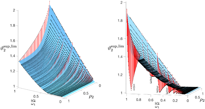
Figure 4: Graph of angular values $\vartheta_{2}^{\sup,\lim}(A(\omega_{1},\omega_{2},\rho_{1},\rho_{2}))$ for the system (42) with matrix from (45) as a function of $\kappa=\frac{\omega_{2}}{\omega_{1}},\rho_{2}\in(0,1]$ for $\rho_{1}=\frac{1}{3}$, $\omega_{1}=1$. At rational values $\kappa=\frac{p}{q}$ with $1\leq p\leq q\leq 20$, $p\perp q$ the vertical line $\{L(t):t\in[0,2\pi]\}$ from (67) is drawn with angular value at the top.

References

- [1] L. Arnold. Random dynamical systems. Springer Monographs in Mathematics. Springer-Verlag, Berlin, 1998.
- [2] L. Barreira. Ergodic theory, hyperbolic dynamics and dimension theory. Universitext. Springer, Heidelberg, 2012.
- [3] H. Bauer. Measure and integration theory, volume 26 of De Gruyter Studies in Mathematics. Walter de Gruyter & Co., Berlin, 2001. Translated from the German by Robert B. Burckel.
- [4] W.-J. Beyn, G. Froyland, and T. Hüls. Angular values of nonautonomous and random linear dynamical systems: Part I—Fundamentals. SIAM J. Appl. Dyn. Syst., 21(2):1245–1286, 2022.
- [5] W.-J. Beyn and T. Hüls. Angular Values of Nonautonomous Linear Dynamical Systems: Part II – Reduction Theory and Algorithm. SIAM J. Appl. Dyn. Syst., 22(1):162–198, 2023.
- [6] A. Björck and G. H. Golub. Numerical methods for computing angles between linear subspaces. Math. Comp., 27:579–594, 1973.
- [7] A. Bunse-Gerstner, R. Byers, V. Mehrmann, and N. K. Nichols. Numerical computation of an analytic singular value decomposition of a matrix valued function. Numer. Math., 60(1):1–39, 1991.
- [8] W. de Melo and S. van Strien. One-dimensional dynamics, volume 25 of Ergebnisse der Mathematik und ihrer Grenzgebiete (3). Springer-Verlag, Berlin, 1993.
- [9] L. Dieci and T. Eirola. On smooth decompositions of matrices. SIAM J. Matrix Anal. Appl., 20(3):800–819, 1999.
- [10] L. Dieci and C. Elia. The singular value decomposition to approximate spectra of dynamical systems. Theoretical aspects. J. Differential Equations, 230(2):502–531, 2006.
- [11] Z. Drmač. On principal angles between subspaces of Euclidean space. SIAM J. Matrix Anal. Appl., 22(1):173–194, 2000.
- [12] L. Eldén and B. Savas. The maximum likelihood estimate in reduced-rank regression. Numer. Linear Algebra Appl., 12(8):731–741, 2005.
- [13] G. H. Golub and C. F. Van Loan. Matrix computations. Johns Hopkins Studies in the Mathematical Sciences. Johns Hopkins University Press, Baltimore, MD, fourth edition, 2013.
- [14] R. A. Horn and C. R. Johnson. Matrix analysis. Cambridge University Press, Cambridge, second edition, 2013.
- [15] S. Jiang. Angles between Euclidean subspaces. Geom. Dedicata, 63(2):113–121, 1996.
- [16] A. B. Katok and B. Hasselblatt. Introduction to the modern theory of dynamical systems. Encyclopedia of mathematics and its applications, vol. 54. Cambridge University Press, Cambridge, 1995.
- [17] R. Lipton, P. Sinz, and M. Stuebner. Angles between subspaces and nearly optimal approximation in GFEM. Comput. Methods Appl. Mech. Engrg., 402:Paper No. 115628, 25, 2022.
- [18] K. Liu, H. Cao, H. C. So, and A. Jakobsson. Multi-dimensional sinusoidal order estimation using angles between subspaces. Digit. Signal Process., 64:17–27, 2017.
- [19] B. Mohammadi. Principal angles between subspaces and reduced order modelling accuracy in optimization. Struct. Multidiscip. Optim., 50(2):237–252, 2014.
- [20] Z. Nitecki. Differentiable dynamics. An introduction to the orbit structure of diffeomorphisms. The M.I.T. Press, Cambridge, Mass.-London, 1971.